Embed Size (px)
Citation preview
Maximum Likelihood Analysis ofPhylogenetic Trees
Benny Chor
School of Computer ScienceTel-Aviv University
Maximum Likelihood Analysis ofPhylogenetic Trees – p.1
Phylogenetic Reconstruction Methods
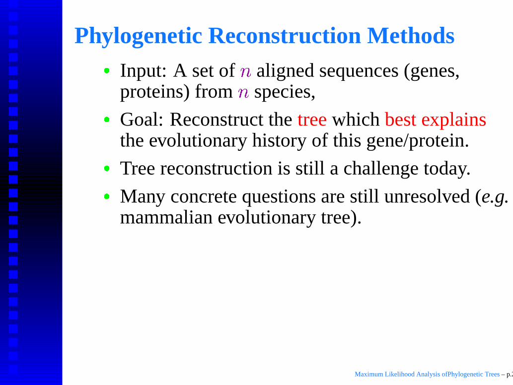
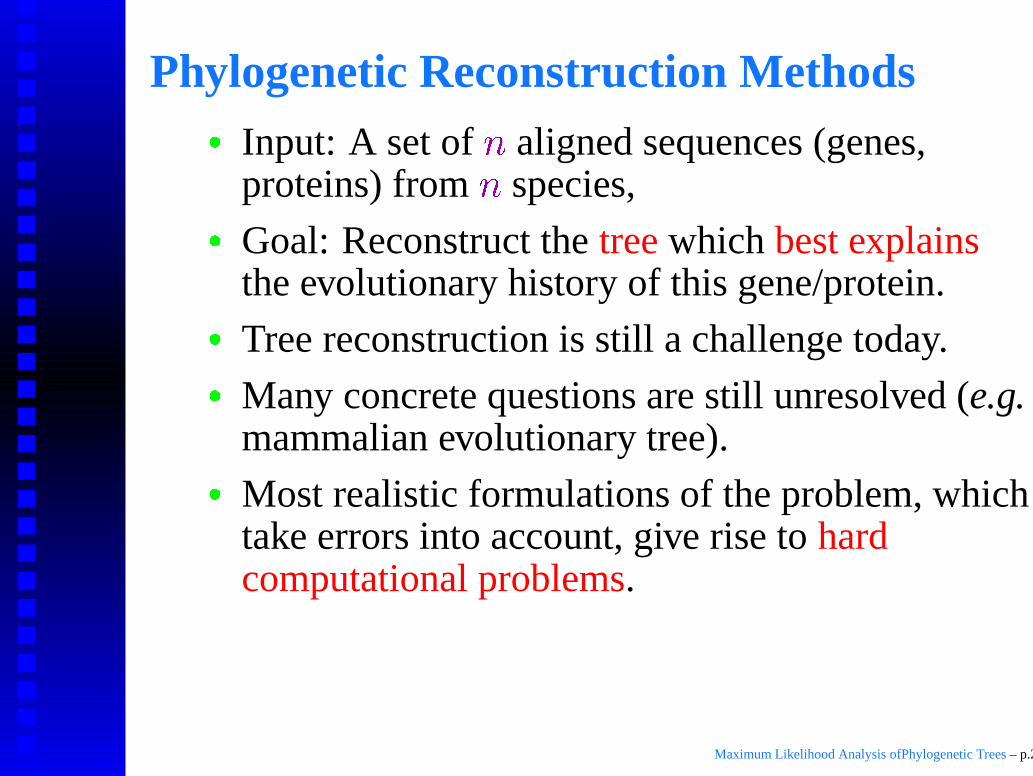
� Input: A set of � aligned sequences (genes,proteins) from � species,
Goal: Reconstruct the tree which best explainsthe evolutionary history of this gene/protein.
Tree reconstruction is still a challenge today.
Many concrete questions are still unresolved (e.g.mammalian evolutionary tree).
Most realistic formulations of the problem, whichtake errors into account, give rise to hardcomputational problems.
Maximum Likelihood Analysis ofPhylogenetic Trees – p.2
Phylogenetic Reconstruction Methods
� Input: A set of � aligned sequences (genes,proteins) from � species,
� Goal: Reconstruct the tree which best explainsthe evolutionary history of this gene/protein.
� Tree reconstruction is still a challenge today.
� Many concrete questions are still unresolved (e.g.mammalian evolutionary tree).
� Most realistic formulations of the problem, whichtake errors into account, give rise to hardcomputational problems.
Maximum Likelihood Analysis ofPhylogenetic Trees – p.2
Popular Reconstruction Methods
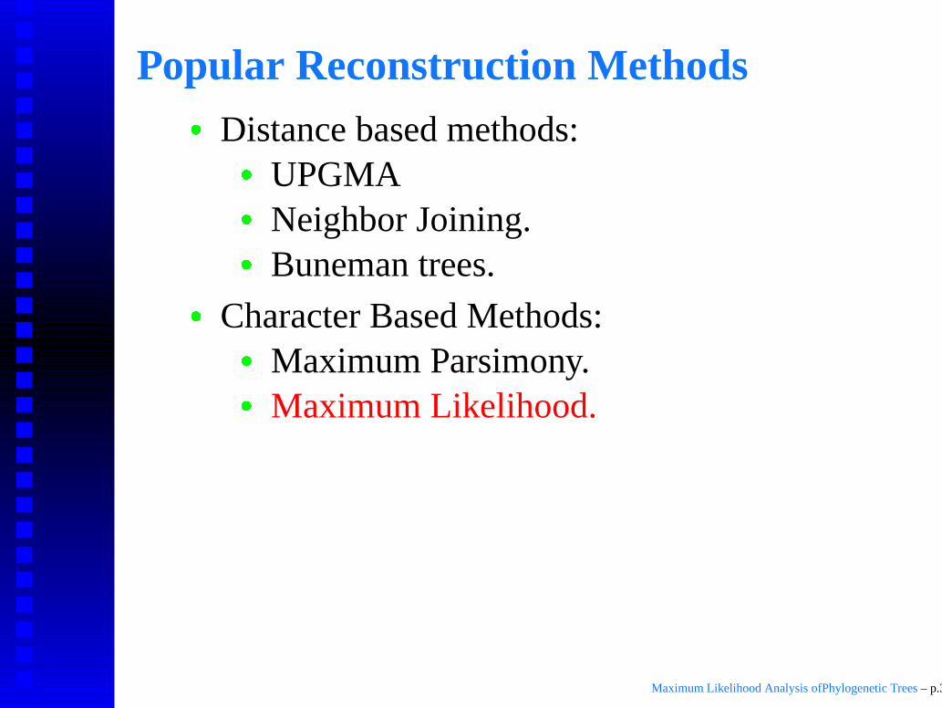
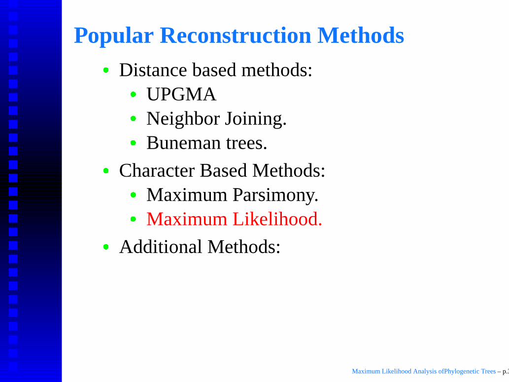
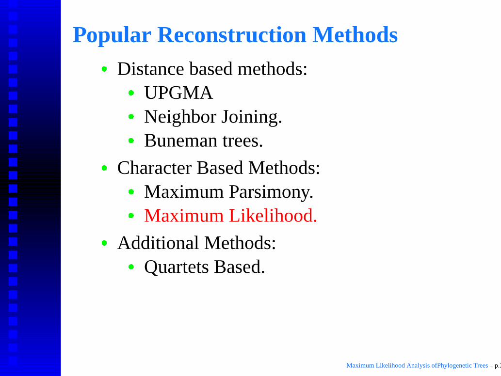
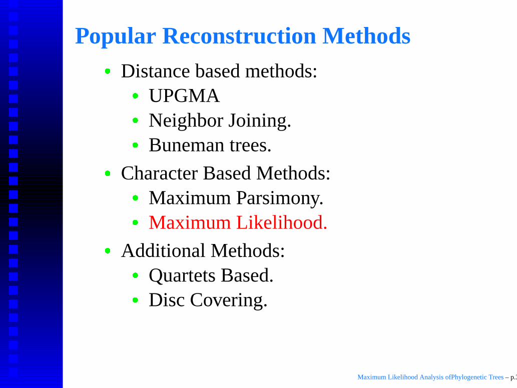
� Distance based methods:
UPGMANeighbor Joining.Buneman trees.
Character Based Methods:Maximum Parsimony.Maximum Likelihood.
Additional Methods:Quartets Based.Disc Covering.
Maximum Likelihood Analysis ofPhylogenetic Trees – p.3
Popular Reconstruction Methods
� Distance based methods:
� UPGMA
Neighbor Joining.Buneman trees.
Character Based Methods:Maximum Parsimony.Maximum Likelihood.
Additional Methods:Quartets Based.Disc Covering.
Maximum Likelihood Analysis ofPhylogenetic Trees – p.3
Popular Reconstruction Methods
� Distance based methods:
� UPGMA
� Neighbor Joining.
Buneman trees.
Character Based Methods:Maximum Parsimony.Maximum Likelihood.
Additional Methods:Quartets Based.Disc Covering.
Maximum Likelihood Analysis ofPhylogenetic Trees – p.3
Popular Reconstruction Methods
� Distance based methods:
� UPGMA
� Neighbor Joining.
� Buneman trees.
Character Based Methods:Maximum Parsimony.Maximum Likelihood.
Additional Methods:Quartets Based.Disc Covering.
Maximum Likelihood Analysis ofPhylogenetic Trees – p.3
Popular Reconstruction Methods
� Distance based methods:
� UPGMA
� Neighbor Joining.
� Buneman trees.
� Character Based Methods:
Maximum Parsimony.Maximum Likelihood.
Additional Methods:Quartets Based.Disc Covering.
Maximum Likelihood Analysis ofPhylogenetic Trees – p.3
Popular Reconstruction Methods
� Distance based methods:
� UPGMA
� Neighbor Joining.
� Buneman trees.
� Character Based Methods:
� Maximum Parsimony.
Maximum Likelihood.
Additional Methods:Quartets Based.Disc Covering.
Maximum Likelihood Analysis ofPhylogenetic Trees – p.3
Popular Reconstruction Methods
� Distance based methods:
� UPGMA
� Neighbor Joining.
� Buneman trees.
� Character Based Methods:
� Maximum Parsimony.
� Maximum Likelihood.
Additional Methods:Quartets Based.Disc Covering.
Maximum Likelihood Analysis ofPhylogenetic Trees – p.3
Popular Reconstruction Methods
� Distance based methods:
� UPGMA
� Neighbor Joining.
� Buneman trees.
� Character Based Methods:
� Maximum Parsimony.
� Maximum Likelihood.
� Additional Methods:
Quartets Based.Disc Covering.
Maximum Likelihood Analysis ofPhylogenetic Trees – p.3
Popular Reconstruction Methods
� Distance based methods:
� UPGMA
� Neighbor Joining.
� Buneman trees.
� Character Based Methods:
� Maximum Parsimony.
� Maximum Likelihood.
� Additional Methods:
� Quartets Based.
Disc Covering.
Maximum Likelihood Analysis ofPhylogenetic Trees – p.3

Popular Reconstruction Methods
� Distance based methods:
� UPGMA
� Neighbor Joining.
� Buneman trees.
� Character Based Methods:
� Maximum Parsimony.
� Maximum Likelihood.
� Additional Methods:
� Quartets Based.
� Disc Covering.
Maximum Likelihood Analysis ofPhylogenetic Trees – p.3

Popular Reconstruction Methods
� Distance based methods:
� UPGMA
� Neighbor Joining.
� Buneman trees.
� Character Based Methods:
� Maximum Parsimony.
� Maximum Likelihood.
� Additional Methods:
� Quartets Based.
� Disc Covering.
Maximum Likelihood Analysis ofPhylogenetic Trees – p.3
Popular Reconstruction Methods
� Distance based methods:
� UPGMA
� Neighbor Joining.
� Buneman trees.
� Character Based Methods:
� Maximum Parsimony.
� Maximum Likelihood.
� Additional Methods:
� Quartets Based.
� Disc Covering.
Maximum Likelihood Analysis ofPhylogenetic Trees – p.3
Talk Outline
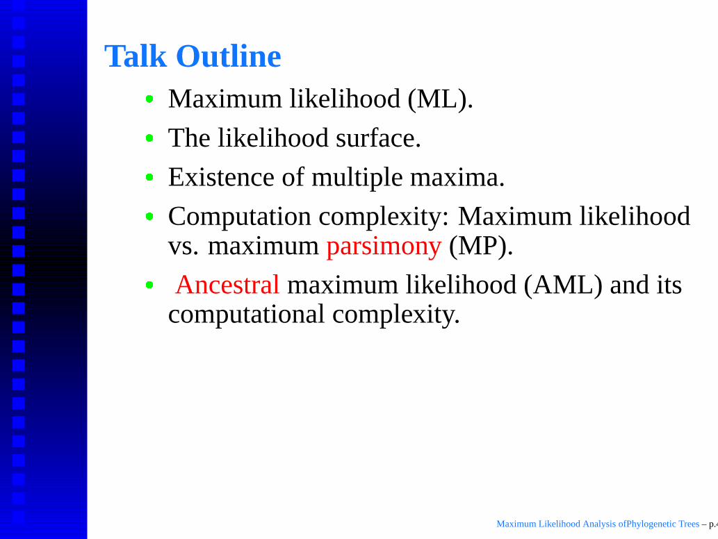
� Maximum likelihood (ML).
The likelihood surface.
Existence of multiple maxima.
Computation complexity: Maximum likelihoodvs. maximum parsimony (MP).
Ancestral maximum likelihood (AML) and itscomputational complexity.
Maximum Likelihood Analysis ofPhylogenetic Trees – p.4
Talk Outline
� Maximum likelihood (ML).
� The likelihood surface.
Existence of multiple maxima.
Computation complexity: Maximum likelihoodvs. maximum parsimony (MP).
Ancestral maximum likelihood (AML) and itscomputational complexity.
Maximum Likelihood Analysis ofPhylogenetic Trees – p.4
Talk Outline
� Maximum likelihood (ML).
� The likelihood surface.
� Existence of multiple maxima.
Computation complexity: Maximum likelihoodvs. maximum parsimony (MP).
Ancestral maximum likelihood (AML) and itscomputational complexity.
Maximum Likelihood Analysis ofPhylogenetic Trees – p.4
Talk Outline
� Maximum likelihood (ML).
� The likelihood surface.
� Existence of multiple maxima.
� Computation complexity: Maximum likelihoodvs. maximum parsimony (MP).
Ancestral maximum likelihood (AML) and itscomputational complexity.
Maximum Likelihood Analysis ofPhylogenetic Trees – p.4
Talk Outline
� Maximum likelihood (ML).
� The likelihood surface.
� Existence of multiple maxima.
� Computation complexity: Maximum likelihoodvs. maximum parsimony (MP).
� Ancestral maximum likelihood (AML) and itscomputational complexity.
Maximum Likelihood Analysis ofPhylogenetic Trees – p.4
Maximum Likelihood
� Input: A set of � observed sequences and anunderlying substitution model.
Desired Output: The weighted tree thatmaximizes the likelihood of the data.
Likelihood of a data: The conditional probabilityof producing the data, given the modelparameters.
Likelihood is a common optimization criteria innumerous settings, including phylogenetic(Felsenstein 1981).
Maximum Likelihood Analysis ofPhylogenetic Trees – p.5
Maximum Likelihood
� Input: A set of � observed sequences and anunderlying substitution model.
� Desired Output: The weighted tree thatmaximizes the likelihood of the data.
� Likelihood of a data: The conditional probabilityof producing the data, given the modelparameters.
Likelihood is a common optimization criteria innumerous settings, including phylogenetic(Felsenstein 1981).
Maximum Likelihood Analysis ofPhylogenetic Trees – p.5
Maximum Likelihood
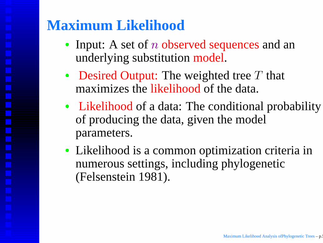
� Input: A set of � observed sequences and anunderlying substitution model.
� Desired Output: The weighted tree thatmaximizes the likelihood of the data.
� Likelihood of a data: The conditional probabilityof producing the data, given the modelparameters.
� Likelihood is a common optimization criteria innumerous settings, including phylogenetic(Felsenstein 1981).
Maximum Likelihood Analysis ofPhylogenetic Trees – p.5
Neyman 2–State Substitution Model
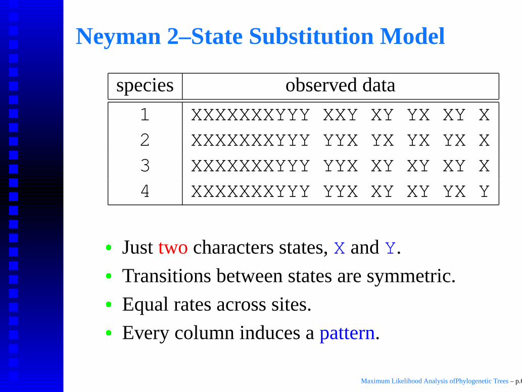
species observed data
1 XXXXXXXYYY XXY XY YX XY X2 XXXXXXXYYY YYX YX YX YX X3 XXXXXXXYYY YYX XY XY XY X4 XXXXXXXYYY YYX XY XY YX Y
� Just two characters states, X and Y.
Transitions between states are symmetric.
Equal rates across sites.
Every column induces a pattern.
Remark: A simple model, yet very powerful.
Maximum Likelihood Analysis ofPhylogenetic Trees – p.6
Neyman 2–State Substitution Model
species observed data
1 XXXXXXXYYY XXY XY YX XY X2 XXXXXXXYYY YYX YX YX YX X3 XXXXXXXYYY YYX XY XY XY X4 XXXXXXXYYY YYX XY XY YX Y
� Just two characters states, X and Y.
� Transitions between states are symmetric.
� Equal rates across sites.
� Every column induces a pattern.
Remark: A simple model, yet very powerful.
Maximum Likelihood Analysis ofPhylogenetic Trees – p.6
Neyman 2–State Substitution Model
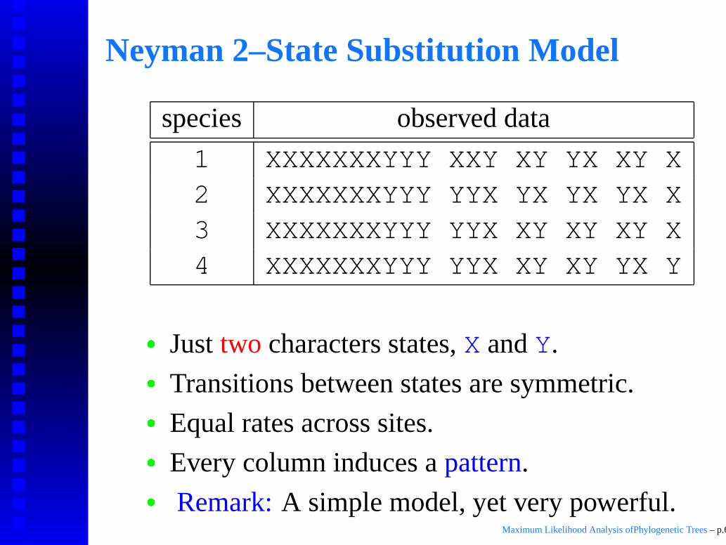
species observed data
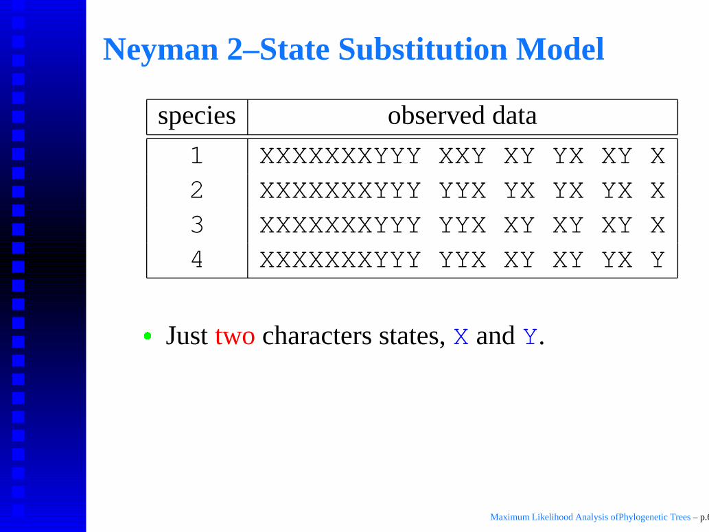
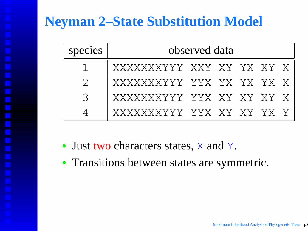
1 XXXXXXXYYY XXY XY YX XY X2 XXXXXXXYYY YYX YX YX YX X3 XXXXXXXYYY YYX XY XY XY X4 XXXXXXXYYY YYX XY XY YX Y
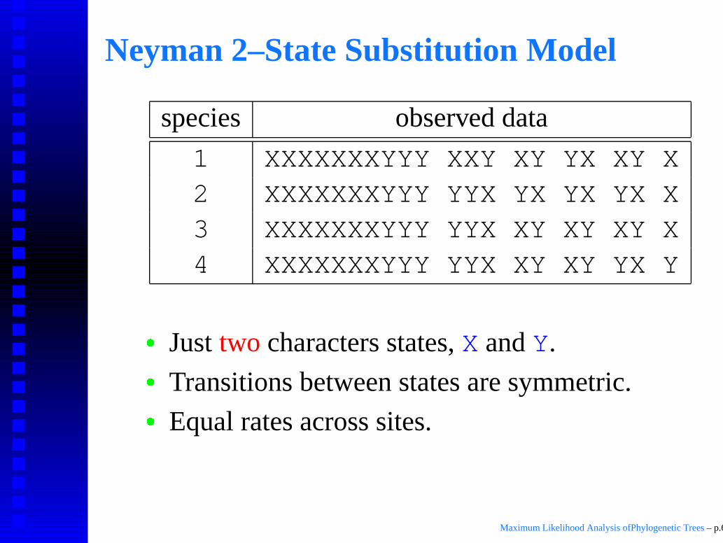
� Just two characters states, X and Y.
� Transitions between states are symmetric.
� Equal rates across sites.
� Every column induces a pattern.
� Remark: A simple model, yet very powerful.Maximum Likelihood Analysis ofPhylogenetic Trees – p.6
Neyman 2–State Substitution Model
��� �
� �� � ���
� � ��
1
2
3
4
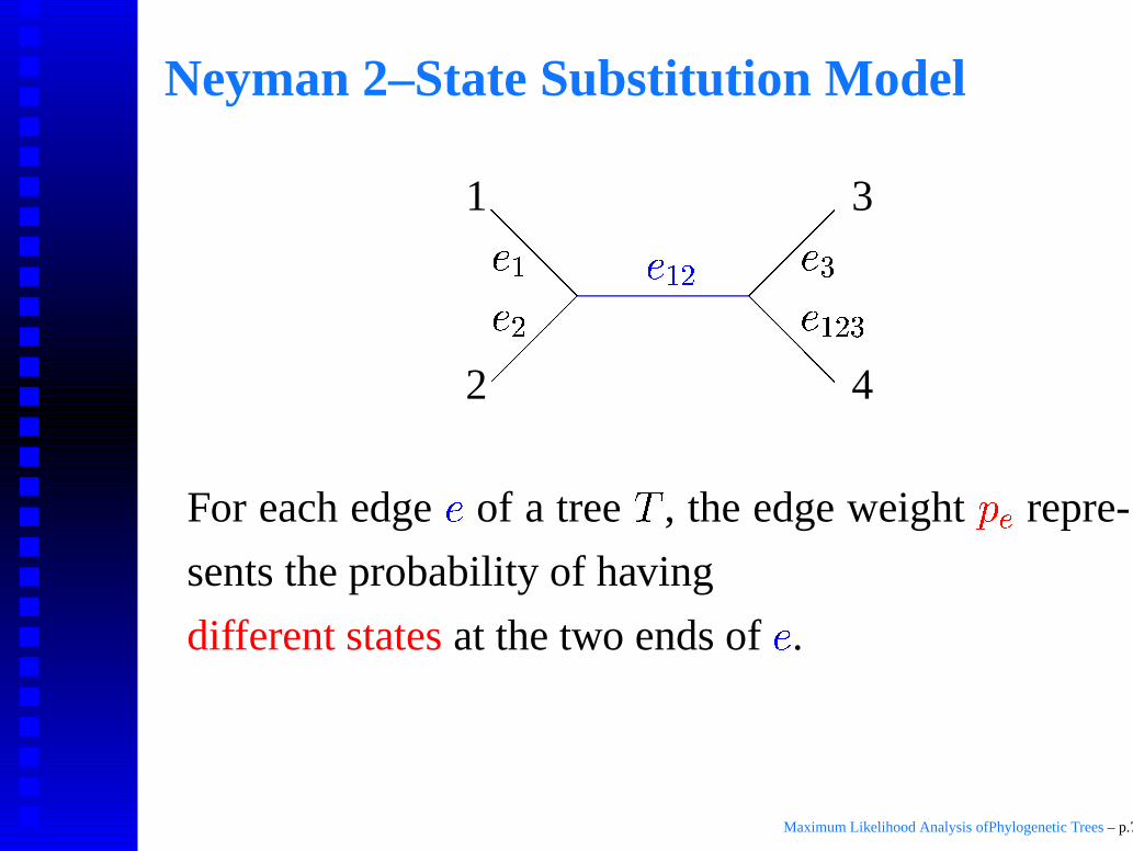
For each edge � of a tree , the edge weight ��� repre-
sents the probability of having
different states at the two ends of �.
Maximum Likelihood Analysis ofPhylogenetic Trees – p.7
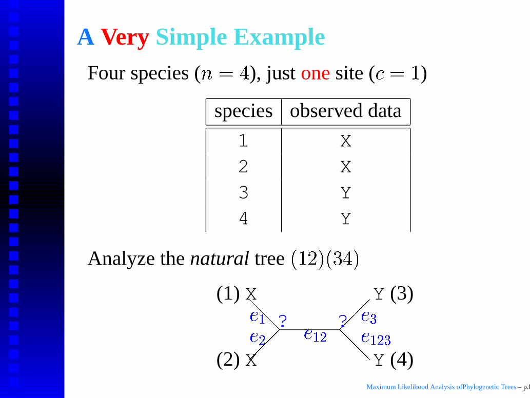
A Very Simple ExampleFour species ( � � �
), just one site ( � � �
)
species observed data
1 X2 X3 Y4 Y
Analyze the natural tree
� �� � ��� � �
� � �� �� � ��
��� ��
(1) X
(2) X
Y (3)
Y (4)
? ?
Maximum Likelihood Analysis ofPhylogenetic Trees – p.8
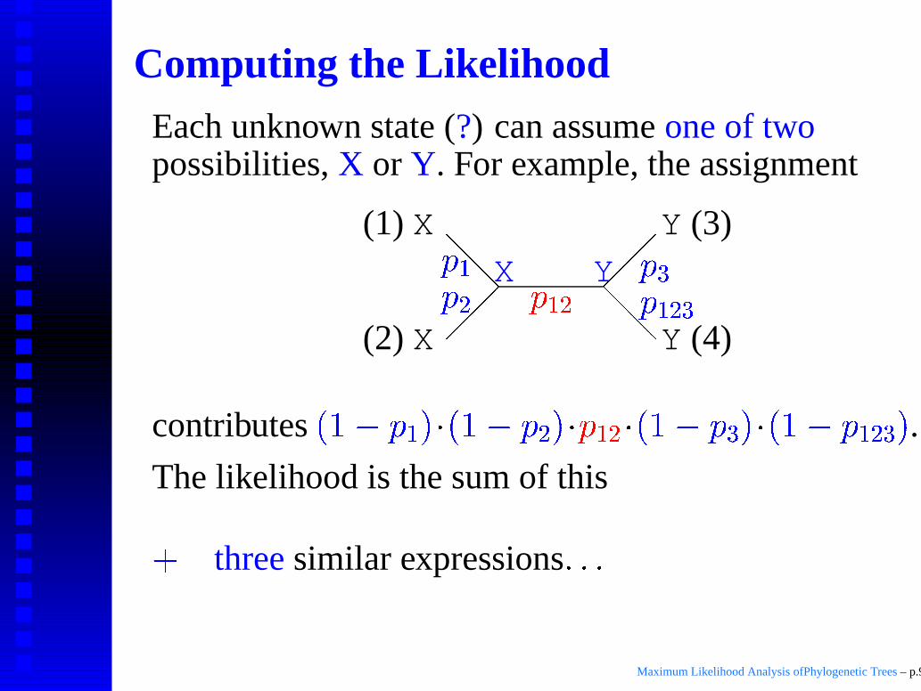
Computing the LikelihoodEach unknown state (?) can assume one of twopossibilities, X or Y. For example, the assignment
�� �� ��� ��
�� ��(1) X
(2) X
Y (3)
Y (4)
X Y
contributes
� �� ��
��
� �� � �
�� �� ��
� �� ��
��
� �� �� ��
�
.
The likelihood is the sum of this
three similar expressions � � �
Maximum Likelihood Analysis ofPhylogenetic Trees – p.9
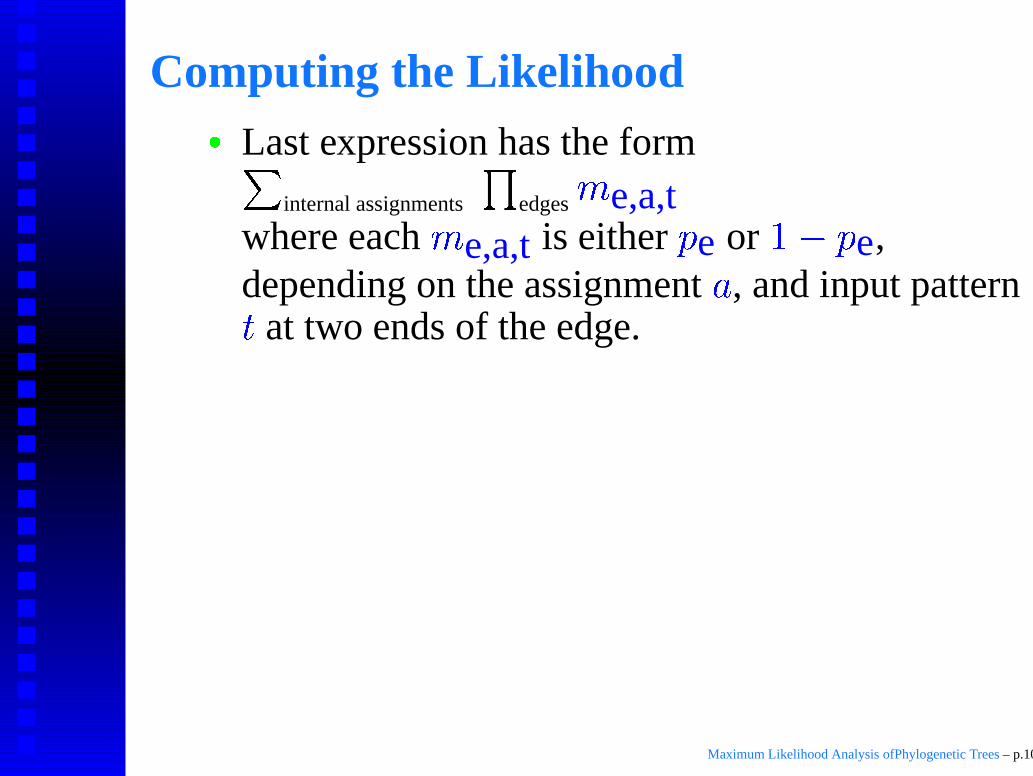
Computing the Likelihood
� Last expression has the form
internal assignments edges
�
e,a,twhere each �
e,a,t is either �
e or�
� �
e,depending on the assignment �, and input pattern
�
at two ends of the edge.
When the data has more then one column, wemultiply the expressions to get the likelihood ofthe data, given the model parameters,
data tree & edge weights :
columns internal assignments edges
e,a,t
Maximum Likelihood Analysis ofPhylogenetic Trees – p.10
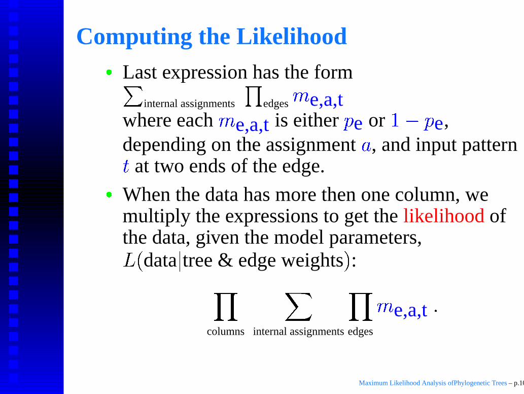
Computing the Likelihood
� Last expression has the form
internal assignments edges
�
e,a,twhere each �
e,a,t is either �
e or�
� �
e,depending on the assignment �, and input pattern
�
at two ends of the edge.
� When the data has more then one column, wemultiply the expressions to get the likelihood ofthe data, given the model parameters,
� �
data
�
tree & edge weights
�
:
columns internal assignments edges
�
e,a,t �
Maximum Likelihood Analysis ofPhylogenetic Trees – p.10
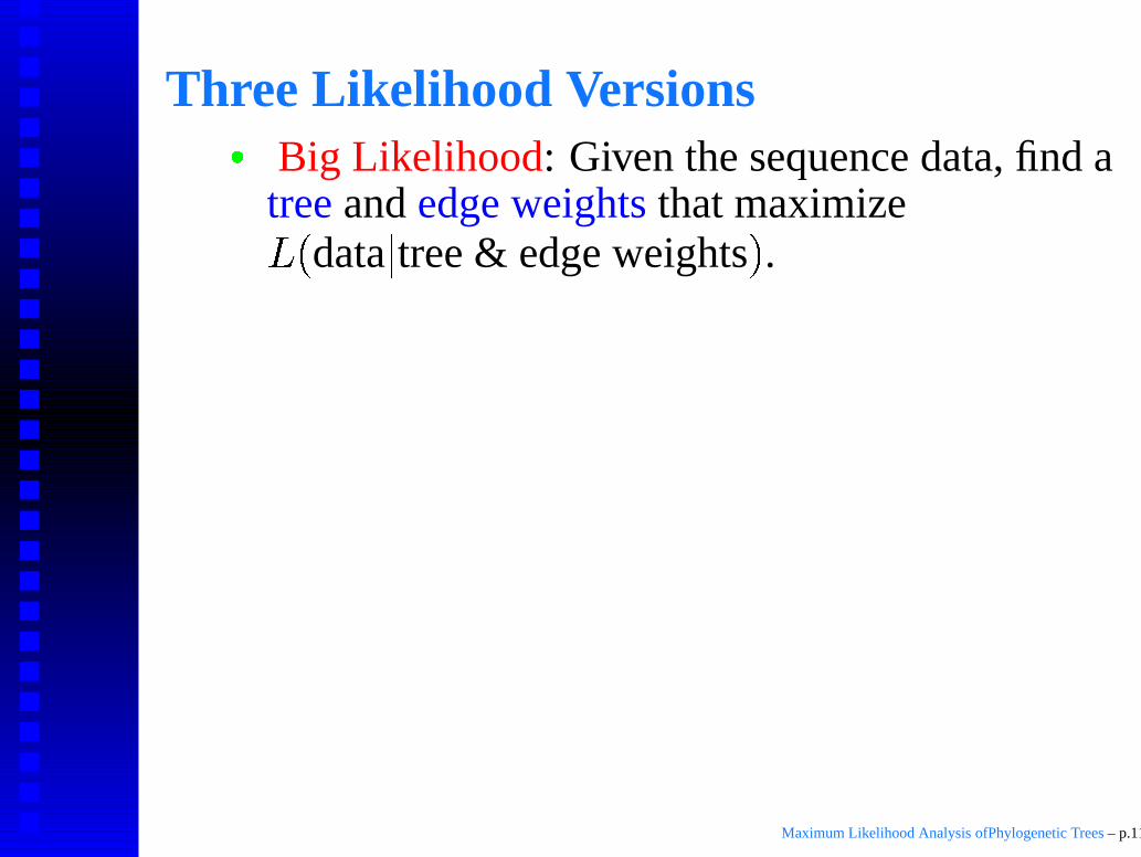
Three Likelihood Versions
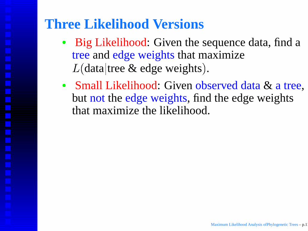
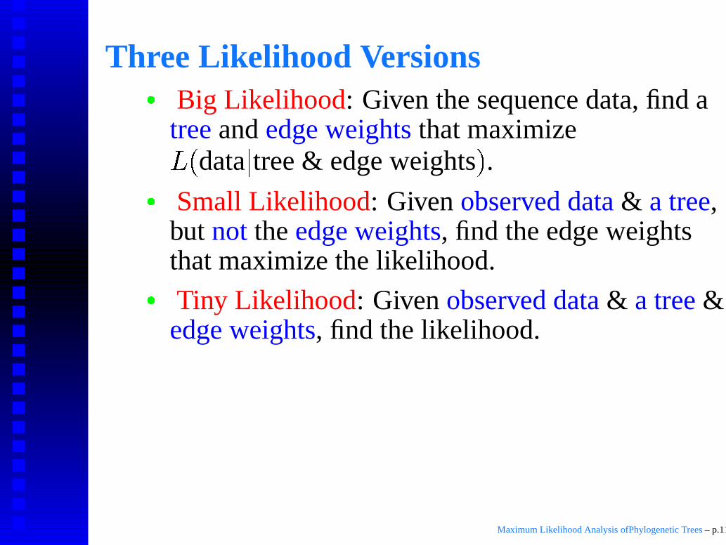
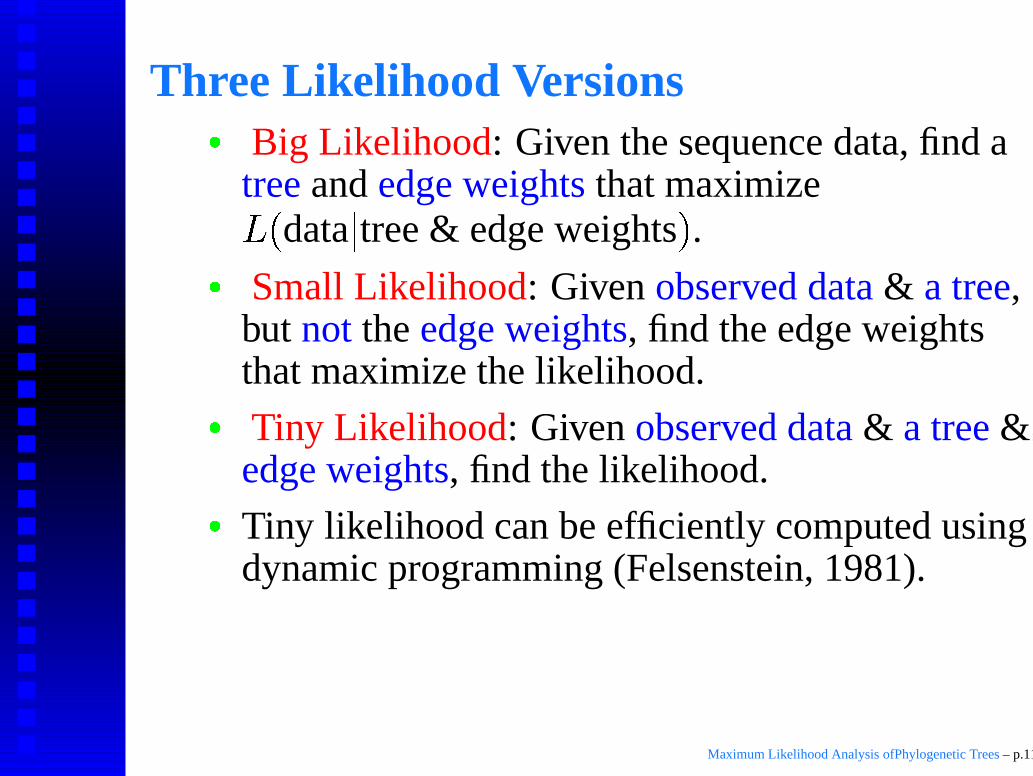
� Big Likelihood: Given the sequence data, find atree and edge weights that maximize
� �
data
�
tree & edge weights
�
.
Small Likelihood: Given observed data & a tree,but not the edge weights, find the edge weightsthat maximize the likelihood.
Tiny Likelihood: Given observed data & a tree &edge weights, find the likelihood.
Tiny likelihood can be efficiently computed usingdynamic programming (Felsenstein, 1981).
Maximum Likelihood Analysis ofPhylogenetic Trees – p.11
Three Likelihood Versions
� Big Likelihood: Given the sequence data, find atree and edge weights that maximize
� �
data
�
tree & edge weights
�
.
� Small Likelihood: Given observed data & a tree,but not the edge weights, find the edge weightsthat maximize the likelihood.
� Tiny Likelihood: Given observed data & a tree &edge weights, find the likelihood.
� Tiny likelihood can be efficiently computed usingdynamic programming (Felsenstein, 1981).
Maximum Likelihood Analysis ofPhylogenetic Trees – p.11
Hill Climbing and Small Likelihood
� Typical approach to small likelihood, used inpractice:
Start at some initial point with edge weights .
Apply hill climbing on the likelihood function toreach a maximum.
Maximum Likelihood Analysis ofPhylogenetic Trees – p.12
Hill Climbing and Small Likelihood
� Typical approach to small likelihood, used inpractice:
� Start at some initial point with edge weights �.
Apply hill climbing on the likelihood function toreach a maximum.
Maximum Likelihood Analysis ofPhylogenetic Trees – p.12
Hill Climbing and Small Likelihood
� Typical approach to small likelihood, used inpractice:
� Start at some initial point with edge weights �.
� Apply hill climbing on the likelihood function toreach a maximum.
Maximum Likelihood Analysis ofPhylogenetic Trees – p.12
The Likelihood Surface
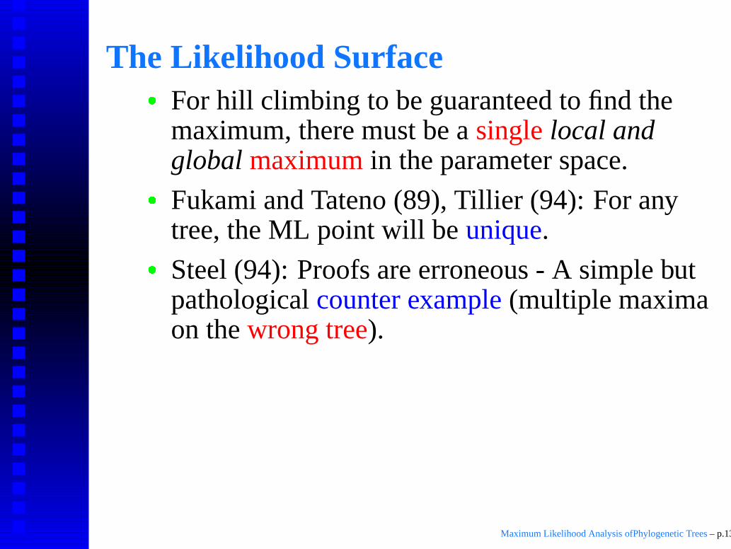
� For hill climbing to be guaranteed to find themaximum, there must be a single local andglobal maximum in the parameter space.
Fukami and Tateno (89), Tillier (94): For anytree, the ML point will be unique.
Steel (94): Proofs are erroneous - A simple butpathological counter example (multiple maximaon the wrong tree).
( –present): Hill climbing techniques still used.Steel’s counter example is considered too“biologically unrealistic” to warrant concern.
Maximum Likelihood Analysis ofPhylogenetic Trees – p.13
The Likelihood Surface
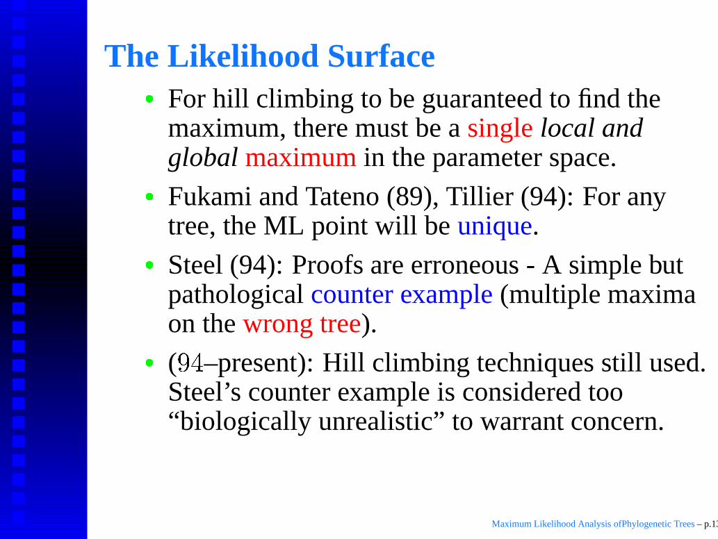
� For hill climbing to be guaranteed to find themaximum, there must be a single local andglobal maximum in the parameter space.
� Fukami and Tateno (89), Tillier (94): For anytree, the ML point will be unique.
Steel (94): Proofs are erroneous - A simple butpathological counter example (multiple maximaon the wrong tree).
( –present): Hill climbing techniques still used.Steel’s counter example is considered too“biologically unrealistic” to warrant concern.
Maximum Likelihood Analysis ofPhylogenetic Trees – p.13
The Likelihood Surface
� For hill climbing to be guaranteed to find themaximum, there must be a single local andglobal maximum in the parameter space.
� Fukami and Tateno (89), Tillier (94): For anytree, the ML point will be unique.
� Steel (94): Proofs are erroneous - A simple butpathological counter example (multiple maximaon the wrong tree).
� (
� �
–present): Hill climbing techniques still used.Steel’s counter example is considered too“biologically unrealistic” to warrant concern.
Maximum Likelihood Analysis ofPhylogenetic Trees – p.13

The Likelihood Surface (cont.)
� Rogers and Swofford (99): Simulation Study
Data is simulated on a tree.Multiple optima are rare......especially on the correct tree.
Goal here: Investigate the problem analytically(joint work with Hendy, Holland, Penny).
Maximum Likelihood Analysis ofPhylogenetic Trees – p.14
The Likelihood Surface (cont.)
� Rogers and Swofford (99): Simulation Study
� Data is simulated on a tree.
Multiple optima are rare......especially on the correct tree.
Goal here: Investigate the problem analytically(joint work with Hendy, Holland, Penny).
Maximum Likelihood Analysis ofPhylogenetic Trees – p.14
The Likelihood Surface (cont.)
� Rogers and Swofford (99): Simulation Study
� Data is simulated on a tree.
� Multiple optima are rare...
...especially on the correct tree.
Goal here: Investigate the problem analytically(joint work with Hendy, Holland, Penny).
Maximum Likelihood Analysis ofPhylogenetic Trees – p.14
The Likelihood Surface (cont.)
� Rogers and Swofford (99): Simulation Study
� Data is simulated on a tree.
� Multiple optima are rare...
� ...especially on the correct tree.
� Goal here: Investigate the problem analytically(joint work with Hendy, Holland, Penny).
Maximum Likelihood Analysis ofPhylogenetic Trees – p.14
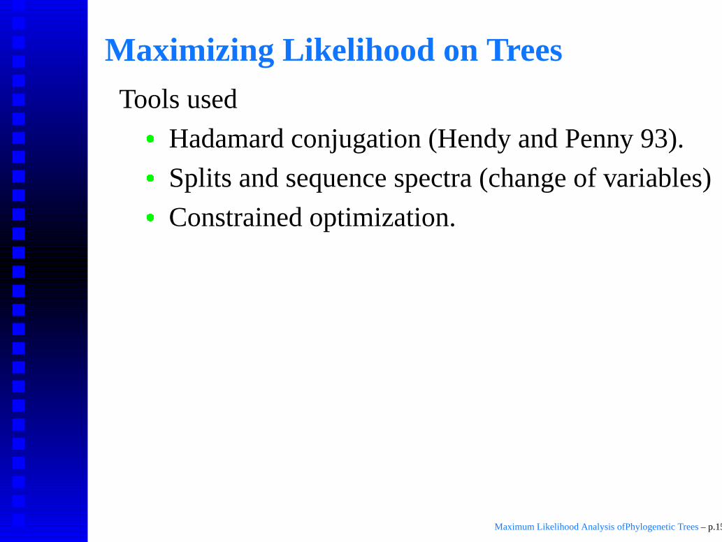
Maximizing Likelihood on TreesTools used
� Hadamard conjugation (Hendy and Penny 93).
Splits and sequence spectra (change of variables)
Constrained optimization.
Systems of polynomial equations.
Analytical solution: very hard in general, evenfor four taxa.
Employing computer algebra and algebraicgeometry tools.
Maximum Likelihood Analysis ofPhylogenetic Trees – p.15
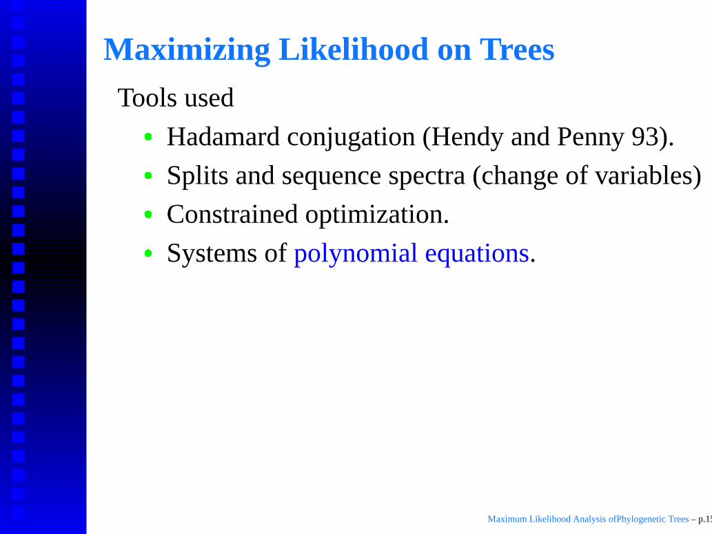
Maximizing Likelihood on TreesTools used
� Hadamard conjugation (Hendy and Penny 93).
� Splits and sequence spectra (change of variables)
Constrained optimization.
Systems of polynomial equations.
Analytical solution: very hard in general, evenfor four taxa.
Employing computer algebra and algebraicgeometry tools.
Maximum Likelihood Analysis ofPhylogenetic Trees – p.15
Maximizing Likelihood on TreesTools used
� Hadamard conjugation (Hendy and Penny 93).
� Splits and sequence spectra (change of variables)
� Constrained optimization.
Systems of polynomial equations.
Analytical solution: very hard in general, evenfor four taxa.
Employing computer algebra and algebraicgeometry tools.
Maximum Likelihood Analysis ofPhylogenetic Trees – p.15
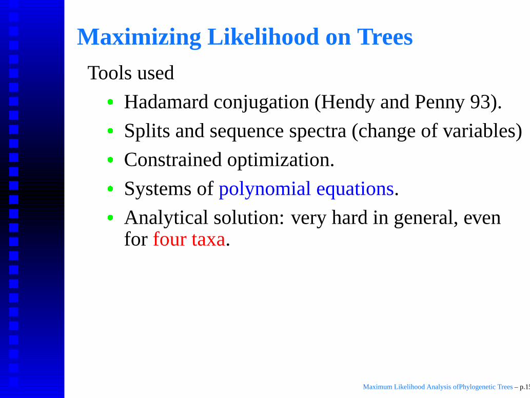
Maximizing Likelihood on TreesTools used
� Hadamard conjugation (Hendy and Penny 93).
� Splits and sequence spectra (change of variables)
� Constrained optimization.
� Systems of polynomial equations.
Analytical solution: very hard in general, evenfor four taxa.
Employing computer algebra and algebraicgeometry tools.
Maximum Likelihood Analysis ofPhylogenetic Trees – p.15
Maximizing Likelihood on TreesTools used
� Hadamard conjugation (Hendy and Penny 93).
� Splits and sequence spectra (change of variables)
� Constrained optimization.
� Systems of polynomial equations.
� Analytical solution: very hard in general, evenfor four taxa.
Employing computer algebra and algebraicgeometry tools.
Maximum Likelihood Analysis ofPhylogenetic Trees – p.15
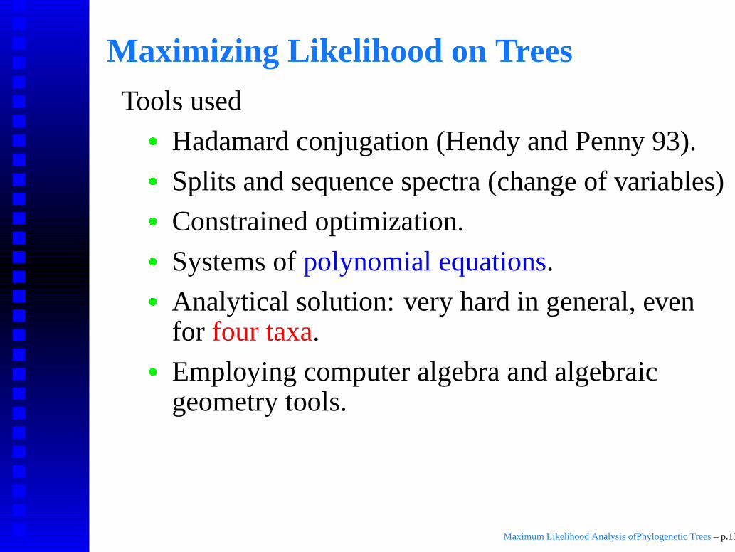
Maximizing Likelihood on TreesTools used
� Hadamard conjugation (Hendy and Penny 93).
� Splits and sequence spectra (change of variables)
� Constrained optimization.
� Systems of polynomial equations.
� Analytical solution: very hard in general, evenfor four taxa.
� Employing computer algebra and algebraicgeometry tools.
Maximum Likelihood Analysis ofPhylogenetic Trees – p.15
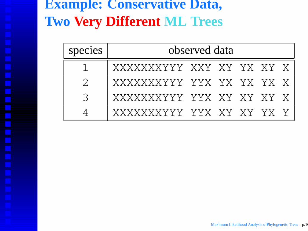
Example: Conservative Data,Two Very Different ML Trees
species observed data
1 XXXXXXXYYY XXY XY YX XY X2 XXXXXXXYYY YYX YX YX YX X3 XXXXXXXYYY YYX XY XY XY X4 XXXXXXXYYY YYX XY XY YX Y
Maximum Likelihood Analysis ofPhylogenetic Trees – p.16
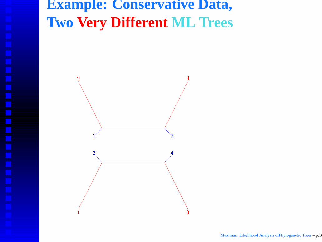
Example: Conservative Data,Two Very Different ML Trees
�
�
�
�
�
�
�
�
���
�
Maximum Likelihood Analysis ofPhylogenetic Trees – p.16
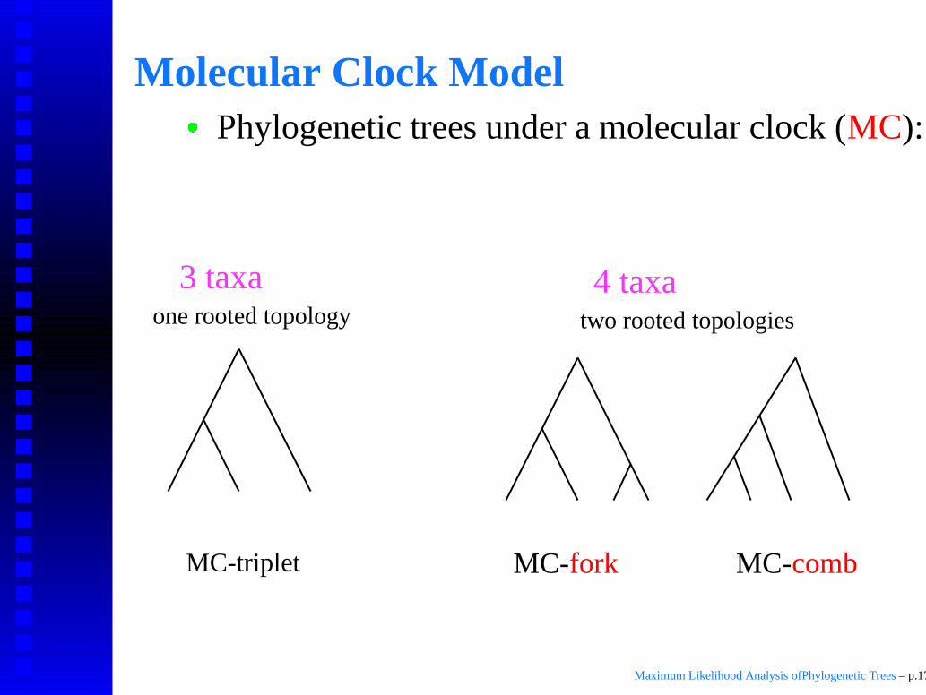
Molecular Clock Model
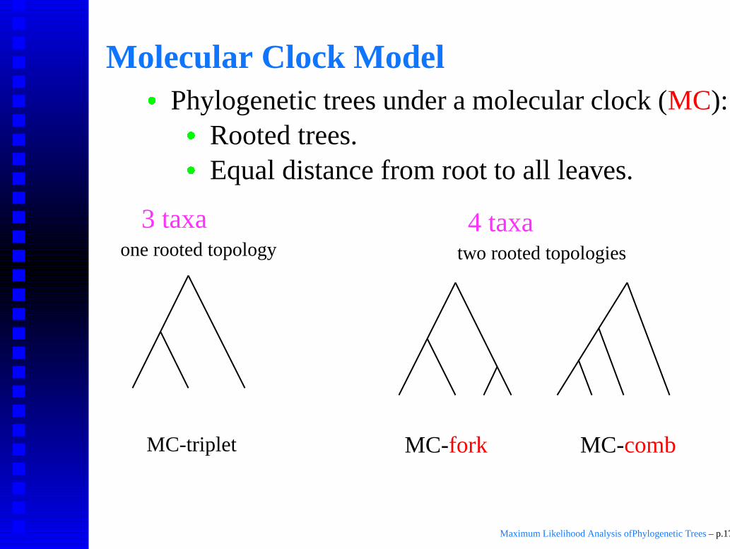
� Phylogenetic trees under a molecular clock (MC):
Rooted trees.Equal distance from root to all leaves.
MC-triplet
one rooted topology two rooted topologies
4 taxa3 taxa
MC-combMC-fork
Maximum Likelihood Analysis ofPhylogenetic Trees – p.17
Molecular Clock Model
� Phylogenetic trees under a molecular clock (MC):
� Rooted trees.
Equal distance from root to all leaves.
MC-triplet
one rooted topology two rooted topologies
4 taxa3 taxa
MC-combMC-fork
Maximum Likelihood Analysis ofPhylogenetic Trees – p.17
Molecular Clock Model
� Phylogenetic trees under a molecular clock (MC):
� Rooted trees.
� Equal distance from root to all leaves.
MC-triplet
one rooted topology two rooted topologies
4 taxa3 taxa
MC-combMC-fork
Maximum Likelihood Analysis ofPhylogenetic Trees – p.17

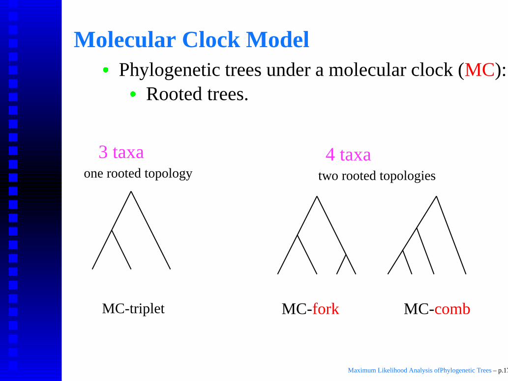
Molecular Clock Model
� Phylogenetic trees under a molecular clock (MC):
� Rooted trees.
� Equal distance from root to all leaves.
MC-triplet
one rooted topology two rooted topologies
4 taxa3 taxa
MC-combMC-fork
Maximum Likelihood Analysis ofPhylogenetic Trees – p.17
Molecular Clock Model
� Phylogenetic trees under a molecular clock (MC):
Rooted trees.Equal distance from root to all leaves.
Negative Examples:
Maximum Likelihood Analysis ofPhylogenetic Trees – p.18
Molecular Clock Model
� Phylogenetic trees under a molecular clock (MC):
� Rooted trees.
Equal distance from root to all leaves.
Negative Examples:
Maximum Likelihood Analysis ofPhylogenetic Trees – p.18
Molecular Clock Model
� Phylogenetic trees under a molecular clock (MC):
� Rooted trees.
� Equal distance from root to all leaves.
Negative Examples:
Maximum Likelihood Analysis ofPhylogenetic Trees – p.18
Molecular Clock Model
� Phylogenetic trees under a molecular clock (MC):
� Rooted trees.
� Equal distance from root to all leaves.
� Negative Examples:
Maximum Likelihood Analysis ofPhylogenetic Trees – p.18
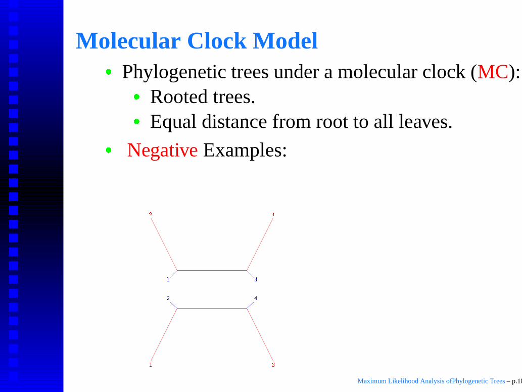
Molecular Clock Model
� Phylogenetic trees under a molecular clock (MC):
� Rooted trees.
� Equal distance from root to all leaves.
� Negative Examples:
�
�
�
�
�
�
�
�
���
�
Maximum Likelihood Analysis ofPhylogenetic Trees – p.18
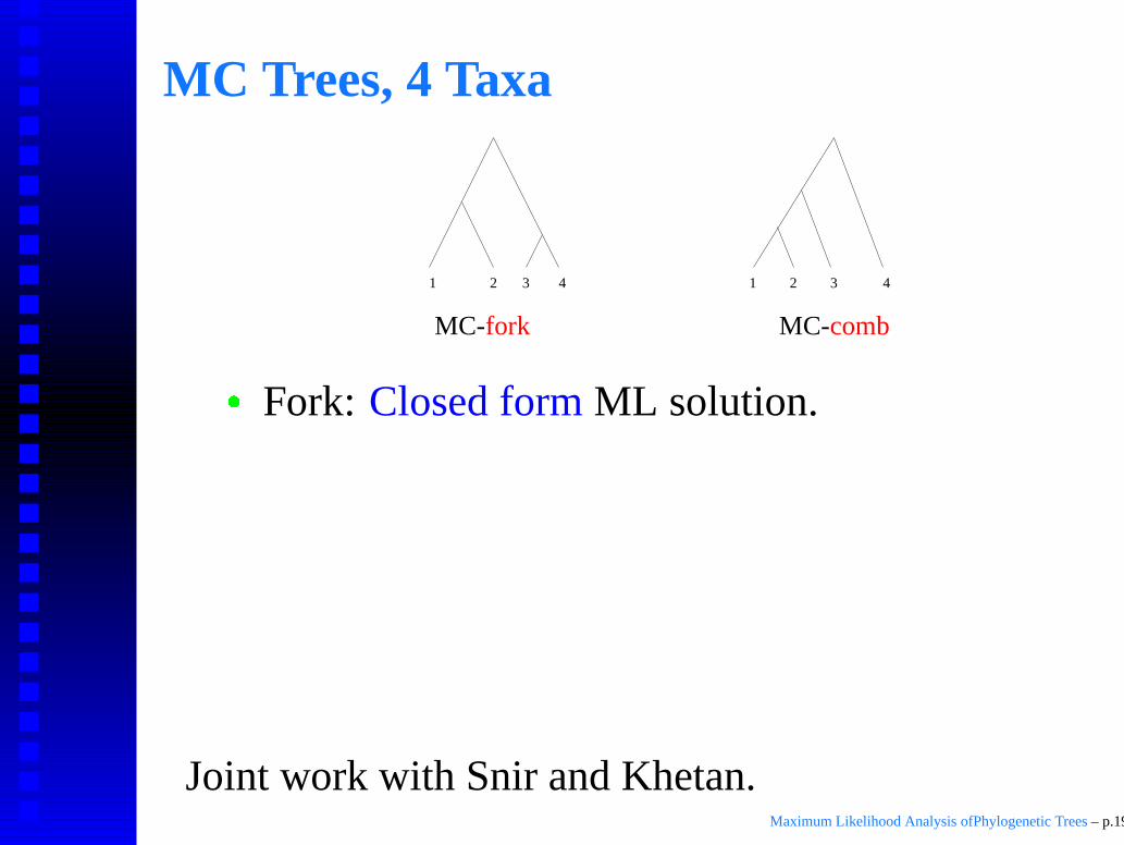
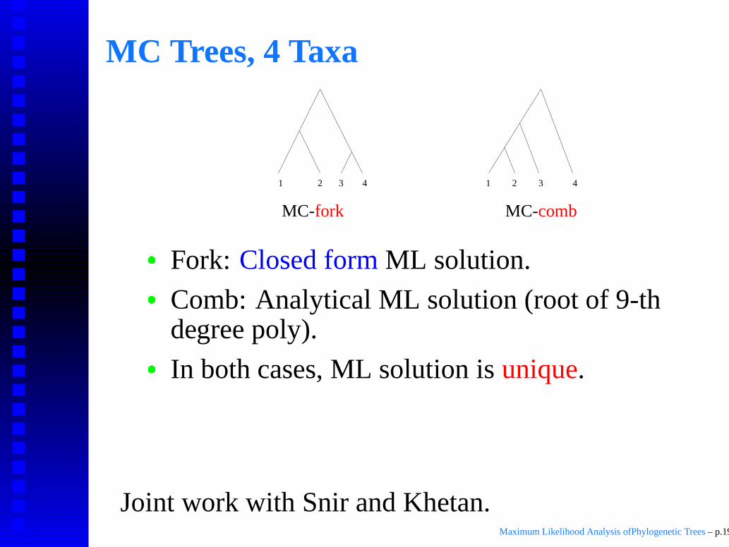
MC Trees, 4 Taxa
2 3 44 2131
MC-fork MC-comb
� Fork: Closed form ML solution.
Comb: Analytical ML solution (root of 9-thdegree poly).
In both cases, ML solution is unique.
Attaining solutions requires fairly heavy mathand computer algebra tools.
Joint work with Snir and Khetan.Maximum Likelihood Analysis ofPhylogenetic Trees – p.19
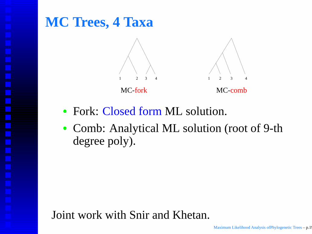
MC Trees, 4 Taxa
2 3 44 2131
MC-fork MC-comb
� Fork: Closed form ML solution.
� Comb: Analytical ML solution (root of 9-thdegree poly).
In both cases, ML solution is unique.
Attaining solutions requires fairly heavy mathand computer algebra tools.
Joint work with Snir and Khetan.Maximum Likelihood Analysis ofPhylogenetic Trees – p.19
MC Trees, 4 Taxa
2 3 44 2131
MC-fork MC-comb
� Fork: Closed form ML solution.
� Comb: Analytical ML solution (root of 9-thdegree poly).
� In both cases, ML solution is unique.
Attaining solutions requires fairly heavy mathand computer algebra tools.
Joint work with Snir and Khetan.Maximum Likelihood Analysis ofPhylogenetic Trees – p.19
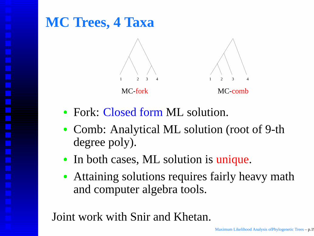
MC Trees, 4 Taxa
2 3 44 2131
MC-fork MC-comb
� Fork: Closed form ML solution.
� Comb: Analytical ML solution (root of 9-thdegree poly).
� In both cases, ML solution is unique.
� Attaining solutions requires fairly heavy mathand computer algebra tools.
Joint work with Snir and Khetan.Maximum Likelihood Analysis ofPhylogenetic Trees – p.19
Small Likelihood & Multiple Maxima
� Small Likelihood (reminder): Given observeddata & a tree, but not the edge weights, find theedge weights that maximize the likelihood.
Multiple ML points for general case imply smalllikelihood cannot be solved by hill climbing.
Not clear if small likelihood has efficient (worstcase) solutions.
Maximum Likelihood Analysis ofPhylogenetic Trees – p.20
Small Likelihood & Multiple Maxima
� Small Likelihood (reminder): Given observeddata & a tree, but not the edge weights, find theedge weights that maximize the likelihood.
� Multiple ML points for general case imply smalllikelihood cannot be solved by hill climbing.
� Not clear if small likelihood has efficient (worstcase) solutions.
Maximum Likelihood Analysis ofPhylogenetic Trees – p.20
Maximum Parsimony (MP)
� Big Parsimony: Given the sequence data, find atree and assignment of sequences to internalnodes that minimizes the number of changesacross all edges.
Small Parsimony: Given the sequence data and atree, find internal assignment(s) that minimizestotal number of changes.
MP considered by practitioners easier than ML.Indeed small parsimony has efficient algorithms(Fitch 1971, Sankoff and Cedergren 1983).
Maximum Likelihood Analysis ofPhylogenetic Trees – p.21
Maximum Parsimony (MP)
� Big Parsimony: Given the sequence data, find atree and assignment of sequences to internalnodes that minimizes the number of changesacross all edges.
� Small Parsimony: Given the sequence data and atree, find internal assignment(s) that minimizestotal number of changes.
� MP considered by practitioners easier than ML.Indeed small parsimony has efficient algorithms(Fitch 1971, Sankoff and Cedergren 1983).
Maximum Likelihood Analysis ofPhylogenetic Trees – p.21
Complexity: MP vs. ML
� Small parsimony is in P.
Small likelihood – unknown.
Big parsimony is NP hard (Day, Johnson andSankoff, 1986).
Big likelihood – unknown. Given the importanceof ML, it would be nice to know more about itscomplexity than just “seems harder than MP”.
Maximum Likelihood Analysis ofPhylogenetic Trees – p.22
Complexity: MP vs. ML
� Small parsimony is in P.
� Small likelihood – unknown.
� Big parsimony is NP hard (Day, Johnson andSankoff, 1986).
� Big likelihood – unknown. Given the importanceof ML, it would be nice to know more about itscomplexity than just “seems harder than MP”.
Maximum Likelihood Analysis ofPhylogenetic Trees – p.22
Ancestral Max. Likelihood (AML)
� A tree reconstruction method that is “in between”ML and MP.
The goal is to simultaneously find edge weightsand assignment of sequences to internal nodes sothat the likelihood of the data, given the treeparameters, is maximized.
AML is widely used in evolutionary studies.
Also termed joint reconstruction of ancestralsequences.
AML computes the likelihood contributionresulting from best assignment to internal nodes,while “regular ML” sums up over allassignments.
Maximum Likelihood Analysis ofPhylogenetic Trees – p.23
Ancestral Max. Likelihood (AML)
� A tree reconstruction method that is “in between”ML and MP.
� The goal is to simultaneously find edge weightsand assignment of sequences to internal nodes sothat the likelihood of the data, given the treeparameters, is maximized.
� AML is widely used in evolutionary studies.
� Also termed joint reconstruction of ancestralsequences.
� AML computes the likelihood contributionresulting from best assignment to internal nodes,while “regular ML” sums up over all assignments.
Maximum Likelihood Analysis ofPhylogenetic Trees – p.23
Two AML Versions
� Big AML: Given the sequence data, find a tree,assignment to internal nodes, and edge weightsthat maximize the likelihood of the data.
Small AML: Given observed data, a tree andedge weights, but not the internal assignment,find the assignment that maximize the likelihood.
PPSG 2000: A poly time, dynamic programmingalgorithm for small AML.
ACHLPW 2003: Big AML is NP-hard.
Maximum Likelihood Analysis ofPhylogenetic Trees – p.24
Two AML Versions
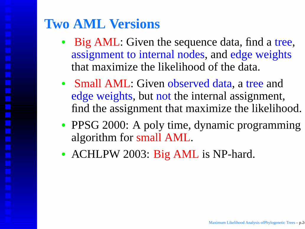
� Big AML: Given the sequence data, find a tree,assignment to internal nodes, and edge weightsthat maximize the likelihood of the data.
� Small AML: Given observed data, a tree andedge weights, but not the internal assignment,find the assignment that maximize the likelihood.
PPSG 2000: A poly time, dynamic programmingalgorithm for small AML.
ACHLPW 2003: Big AML is NP-hard.
Maximum Likelihood Analysis ofPhylogenetic Trees – p.24
Two AML Versions
� Big AML: Given the sequence data, find a tree,assignment to internal nodes, and edge weightsthat maximize the likelihood of the data.
� Small AML: Given observed data, a tree andedge weights, but not the internal assignment,find the assignment that maximize the likelihood.
� PPSG 2000: A poly time, dynamic programmingalgorithm for small AML.
� ACHLPW 2003: Big AML is NP-hard.
Maximum Likelihood Analysis ofPhylogenetic Trees – p.24
Useful AML Observation
� Given sequence data, a tree, and assignment tointernal nodes.
The edge weights that maximize the likelihood ofthe data equal .
Where equals the number of changes accrossedge , and is the common sequence length.
Maximum Likelihood Analysis ofPhylogenetic Trees – p.25
Useful AML Observation
� Given sequence data, a tree, and assignment tointernal nodes.
� The edge weights that maximize the likelihood ofthe data equal
��
��
.
Where equals the number of changes accrossedge , and is the common sequence length.
Maximum Likelihood Analysis ofPhylogenetic Trees – p.25
Useful AML Observation
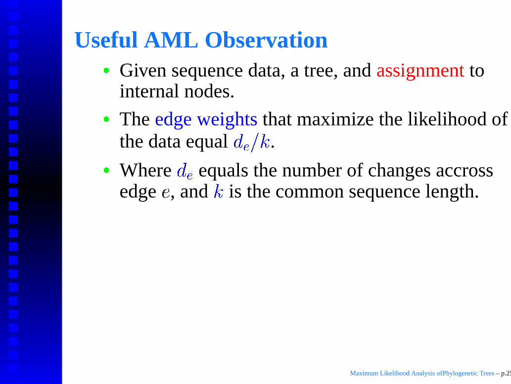
� Given sequence data, a tree, and assignment tointernal nodes.
� The edge weights that maximize the likelihood ofthe data equal
��
��
.
� Where
�� equals the number of changes accross
edge �, and
�
is the common sequence length.
Maximum Likelihood Analysis ofPhylogenetic Trees – p.25
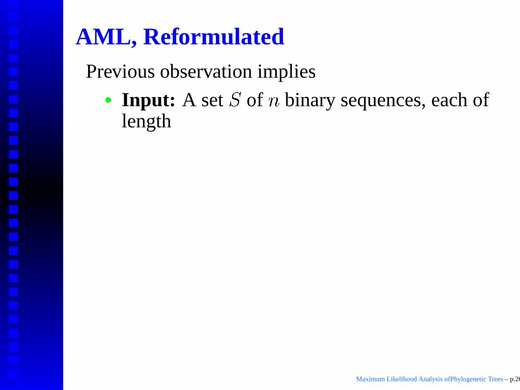
AML, ReformulatedPrevious observation implies
� Input: A set
�
of � binary sequences, each oflength
Goal: Find a tree with leaves, an assignmentof edge probabilities, and a
labelling of the vertices suchthat1. The labels of the leaves are exactly the
sequences from .2. the sum of all “edge entropies”
is minimized.
Maximum Likelihood Analysis ofPhylogenetic Trees – p.26
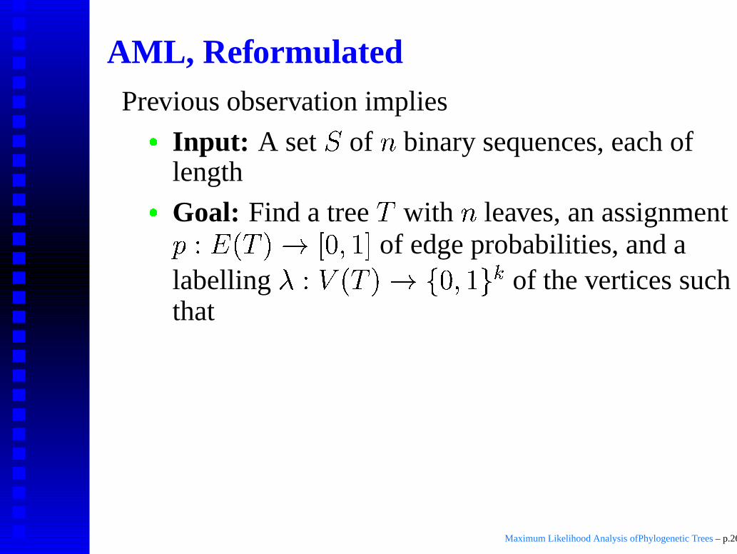
AML, ReformulatedPrevious observation implies
� Input: A set
�
of � binary sequences, each oflength
� Goal: Find a tree with � leaves, an assignment
��
� � � ��
� �
of edge probabilities, and alabelling
� �
� � � ��
� � �
of the vertices suchthat
1. The labels of the leaves are exactly thesequences from .
2. the sum of all “edge entropies”is minimized.
Maximum Likelihood Analysis ofPhylogenetic Trees – p.26
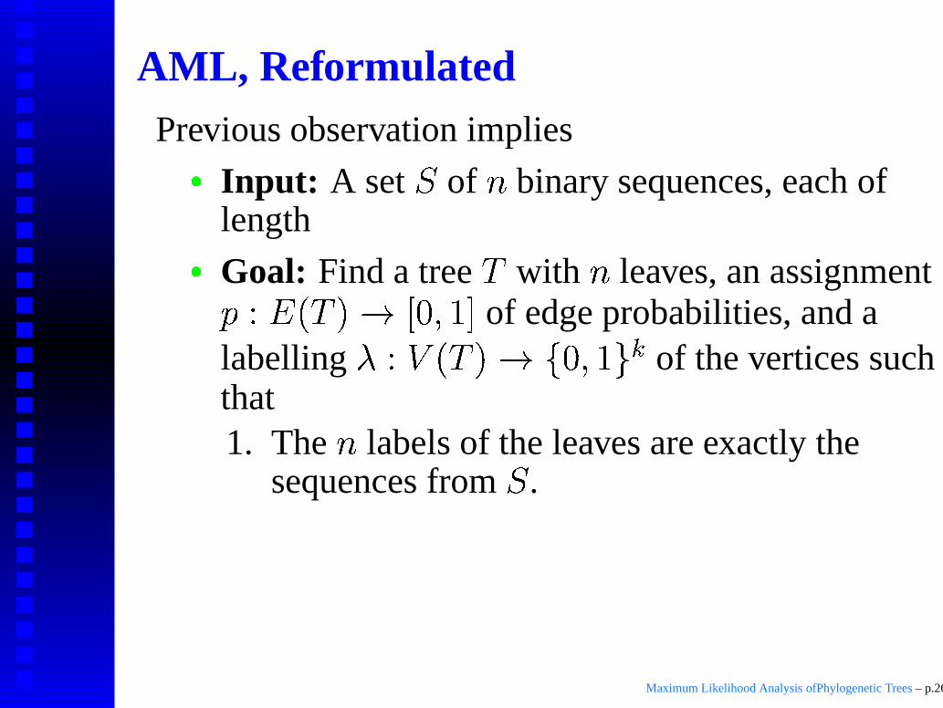
AML, ReformulatedPrevious observation implies
� Input: A set
�
of � binary sequences, each oflength
� Goal: Find a tree with � leaves, an assignment
��
� � � ��
� �
of edge probabilities, and alabelling
� �
� � � ��
� � �
of the vertices suchthat1. The � labels of the leaves are exactly the
sequences from
�
.
2. the sum of all “edge entropies”is minimized.
Maximum Likelihood Analysis ofPhylogenetic Trees – p.26
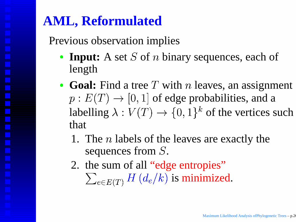
AML, ReformulatedPrevious observation implies
� Input: A set
�
of � binary sequences, each oflength
� Goal: Find a tree with � leaves, an assignment
��
� � � ��
� �
of edge probabilities, and alabelling
� �
� � � ��
� � �
of the vertices suchthat1. The � labels of the leaves are exactly the
sequences from
�
.2. the sum of all “edge entropies”
� � � �� �
� ��
�� �
is minimized.
Maximum Likelihood Analysis ofPhylogenetic Trees – p.26
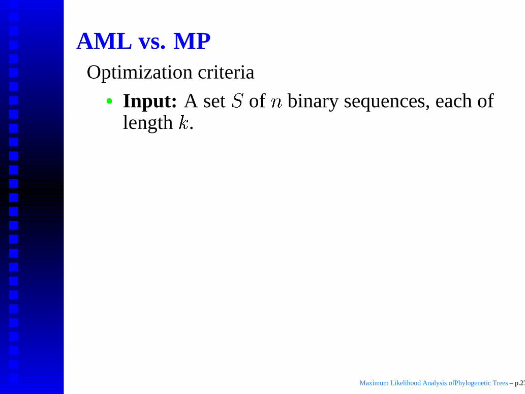
AML vs. MPOptimization criteria
� Input: A set
�
of � binary sequences, each oflength
�
.
AML: Minimize the sum of all “edge entropies”.
MP: Minimize the sum of all “edge differences”.
Can think of the two problems as attempting tominimize different edge weights (functions of
).
Maximum Likelihood Analysis ofPhylogenetic Trees – p.27
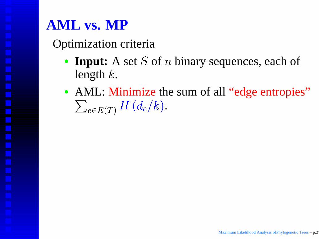
AML vs. MPOptimization criteria
� Input: A set
�
of � binary sequences, each oflength
�
.
� AML: Minimize the sum of all “edge entropies”
� � � � � �
� ��
�� �
.
� MP: Minimize the sum of all “edge differences”
� � � � � � ��
��
.
Can think of the two problems as attempting tominimize different edge weights (functions of
).
Maximum Likelihood Analysis ofPhylogenetic Trees – p.27
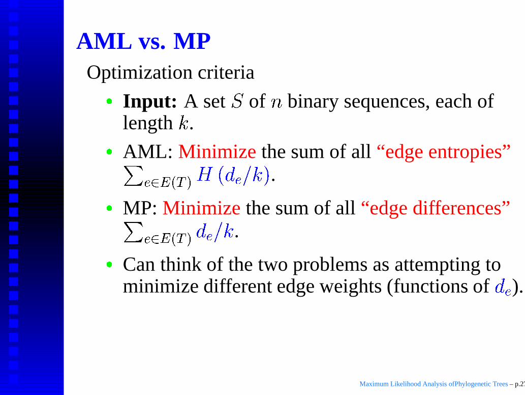
AML vs. MPOptimization criteria
� Input: A set
�
of � binary sequences, each oflength
�
.
� AML: Minimize the sum of all “edge entropies”
� � � � � �
� ��
�� �
.
� MP: Minimize the sum of all “edge differences”
� � � � � � ��
��
.
� Can think of the two problems as attempting tominimize different edge weights (functions of
�� ).
Maximum Likelihood Analysis ofPhylogenetic Trees – p.27
NP hardness of AML: Ideas
� MP was shown NP-hard by Day, Johnson,Sankoff using reduction from vertex cover (VC).
Analogy of AML and MP optimization criteriasuggests using similar approach.
Reduction from VC indeed identical.
Proof substantially more involved as entropyis not as “well behaved” as plain edge
differences .
Maximum Likelihood Analysis ofPhylogenetic Trees – p.28
NP hardness of AML: Ideas
� MP was shown NP-hard by Day, Johnson,Sankoff using reduction from vertex cover (VC).
� Analogy of AML and MP optimization criteriasuggests using similar approach.
� Reduction from VC indeed identical.
� Proof substantially more involved as entropy� ��
�� �
is not as “well behaved” as plain edgedifferences
��
��
.
Maximum Likelihood Analysis ofPhylogenetic Trees – p.28
Conclusion and Open Problems
� Analytic solutions to additional ML problemswith few taxa may be feasible, and may revealadditional properties of likelihood surface (e.g.number of local maxima).
Multiple ML points for MC trees with more than4 taxa?
Hardness proof for big AML as a stepping stonefor big ML?
Is small ML in poly-time?
Thank you!
Maximum Likelihood Analysis ofPhylogenetic Trees – p.29
Conclusion and Open Problems
� Analytic solutions to additional ML problemswith few taxa may be feasible, and may revealadditional properties of likelihood surface (e.g.number of local maxima).
� Multiple ML points for MC trees with more than4 taxa?
� Hardness proof for big AML as a stepping stonefor big ML?
� Is small ML in poly-time?
Thank you!
Maximum Likelihood Analysis ofPhylogenetic Trees – p.29