Embed Size (px)
Citation preview
Maximum Likelihood Based Estimation of Hazard Function under Shape
Restrictions and Related Statistical Inference
by
Desale Habtzghi
(Under the direction of Somnath Datta and Mary Meyer )
Abstract
The problem of estimation of a hazard function has received considerable attention in
the statistical literature. In particular, assumptions of increasing, decreasing, concave and
bathtub-shaped hazard function are common in literature, but practical solutions are not well
developed. In this dissertation, we introduce a new nonparametric method for estimation of
hazard function under shape restrictions to handle the above problem. This is an important
topic of practical utility because often, in survival analysis and reliability applications, one
has a prior notion about the physical shape of underlying hazard rate function. At the
same time, it may not be appropriate to assume a totally parametric form for it. We adopt
a nonparametric approach in assuming that the density and hazard rate have no specific
parametric form with the assumption that the shape of the underlying hazard rate is known
( either decreasing, increasing, concave, convex or bathtub-shaped). We present an efficient
algorithm for computing the shape restricted estimator. The theoretical justification for the
algorithm is provided. We also show how the estimation procedures can be used when dealing

with right censored data. We evaluate the performance of the estimator via simulation studies
and illustrate it on some real data sets.
We also consider testing the hypothesis that the lifetimes come from a population with a
parametric hazard rate such as Weibull against a shape restricted alternative which comprises
a broad range of hazard rate shapes. The alternative may be appropriate when the shape of
the parametric hazard is not constant and monotone. We use appropriate resampling based
computation to conduct our tests since the asymptotic distributions of the test statistics in
these problems are mostly intractable.
Index words: Survival Analysis, Hazard Function, Survival Function, Right CensoredData, Nonparametric, Estimation, Parametric, increasing, decreasing,Bathtub-Shaped, Concave, Shape Restricted Estimator, Simulation,Testing, Resampling.
Maximum Likelihood Based Estimation of Hazard Function under Shape
Restrictions and Related Statistical Inference
by
Desale Habtzghi
B.S., University of Asmara, Eritrea, 1996
M.S., Southern Illinois University, U.S.A, 2001
M.S., University of Georgia, U.S.A, 2003
A Dissertation Submitted to the Graduate Faculty
of The University of Georgia in Partial Fulfillment
of the
Requirements for the Degree
DOCTOR OF PHILOSOPHY
Athens, Georgia
2006

c© 2006
Desale Habtzghi
All Rights Reserved
Maximum Likelihood Based Estimation of Hazard Function under Shape
Restrictions and Related Statistical Inference
by
Desale Habtzghi
Approved:
Major Professor: Somnath Datta and Mary Meyer
Committee: Ishwar Basawa
Daniel Hall
Lynne Seymour
Electronic Version Approved:
Maureen Grasso
Dean of the Graduate School
The University of Georgia
May 2006

Dedication
To my brother Hagos Hadera Habtzghi
iv

Acknowledgments
Writing acknowledgments is a time to reflect upon the glorious struggle that has just taken
place and remember each step along the way. At every turn there are many who have given
their time, energy and expertise and I wish to thank each for the help.
I would like to express my sincere appreciation to my major professors, Dr. Somnath
Datta and Dr. Mary Meyer, who provided not only the direction for the project, but also an
enthusiasm and personal concern which greatly contributed to its progress. Dr. Meyer’s inno-
vative ideas have provided me with a new research avenue and a desire to learn more about
the nonparametric function estimation using shape restrictions. I appreciate her endless help
in pushing me to fully understand the concepts of shape restrictions, without her open door,
open mind and potential it is impossible to complete this project. Dr. Datta broadened my
horizons, I particularly would like to thank him for helping to open my eyes to biostatistics
discipline. I really appreciate all the inputs, advice and encouragement I got from him. He
is always there for me when I call him.
I would like to thank Dr. Ishwar Basawa, Dr. Daniel Hall and Dr. Lynne Seymour for
serving on my committee as well as for their comments and enhancing my professional
development. I am grateful to have spent five years with most knowledgeable professors and
the most friendly staff as well as fellow students, building my solid professional background.
In particular, I would like to thank Dr. Seymour for teaching me Fortran 90 while I was
taking Stat 8060.
v

vi
I would like to express my appreciation to Dr. Robert Lund, Dr. Robert Taylor, Dr.
Tharuvai Sriram and Dr. John Stufken for allowing me to teach in the department of statis-
tics. I would like to Thank Dr. Pike for always wishing me the best.
I am especially appreciative of the support and love of several friends including Mehari,
Thomas, Tesfay, Ron, Musie, Simon, Mebrahtu, Aman, Abel, J. Park, Ross, Archan, Haitao,
Lin Lin, Ghenet, Helen, Dipankar and others who made it easy to live away from home.
I thank my parents for always being there for me. Finally, I would like to express my
sincere thanks to my relatives for their endless love and support. Above all, my highest
gratitude to my God.
I would like to dedicate this dissertation to the memory of my brother, Hagos, who has
passed away because of a tragic accident in 2002.
Table of Contents
Page
Acknowledgments . . . . . . . . . . . . . . . . . . . . . . . . . . . . . . . . . v
List of Tables . . . . . . . . . . . . . . . . . . . . . . . . . . . . . . . . . . . ix
List of Figures . . . . . . . . . . . . . . . . . . . . . . . . . . . . . . . . . . . xi
Chapter
1 INTRODUCTION . . . . . . . . . . . . . . . . . . . . . . . . . . . . . 1
2 LITERATURE REVIEW . . . . . . . . . . . . . . . . . . . . . . . . . 6
2.1 Distribution of failure time . . . . . . . . . . . . . . . . . . 6
2.2 Censoring . . . . . . . . . . . . . . . . . . . . . . . . . . . . . . 9
2.3 Estimation . . . . . . . . . . . . . . . . . . . . . . . . . . . . . . 10
2.4 Shape Restricted Regression . . . . . . . . . . . . . . . . . . 15
3 ESTIMATION OF HAZARD FUNCTION UNDER SHAPE RESTRIC-
TIONS . . . . . . . . . . . . . . . . . . . . . . . . . . . . . . . . . . . . 27
3.1 Uncensored Sample . . . . . . . . . . . . . . . . . . . . . . . . 27
3.2 Computing the Estimator . . . . . . . . . . . . . . . . . . . . 31
3.3 Examples . . . . . . . . . . . . . . . . . . . . . . . . . . . . . . 39
3.4 Right Censored Sample . . . . . . . . . . . . . . . . . . . . . 43
4 SIMULATION STUDIES AND APPLICATION TO REAL DATA
SETS . . . . . . . . . . . . . . . . . . . . . . . . . . . . . . . . . . . . . 49
vii
viii
4.1 Simulation Results . . . . . . . . . . . . . . . . . . . . . . . . 49
4.2 Application To Real Data Sets . . . . . . . . . . . . . . . . . 52
5 TESTING FOR SHAPE RESTRICTED HAZARD FUNCTION
USING RESAMPLING TECHNIQUES . . . . . . . . . . . . . . . . . 62
5.1 Test Statistics . . . . . . . . . . . . . . . . . . . . . . . . . . . 64
5.2 Resampling Approach . . . . . . . . . . . . . . . . . . . . . . . 66
5.3 Bootstrap based tests . . . . . . . . . . . . . . . . . . . . . . 68
5.4 Simulation Studies and Results . . . . . . . . . . . . . . . . . 70
6 CONCLUSIONS AND FUTURE RESEARCH . . . . . . . . . . . . . 77
6.1 Summary . . . . . . . . . . . . . . . . . . . . . . . . . . . . . . . 77
6.2 Bayesian Approach To Shape Restricted Hazard Function 77
6.3 Marginal Estimation of Hazard Function Under Shape
Restriction in Presence of Dependent Censoring . . . . . 79
6.4 Hazard Function Estimation Using Splines Under Shape
Restrictions . . . . . . . . . . . . . . . . . . . . . . . . . . . . 80
Bibliography . . . . . . . . . . . . . . . . . . . . . . . . . . . . . . . . . . . . 83
Appendix
A Head and Neck Cancer data for Arm A . . . . . . . . . . . . . . . 89
B Bone Marrow Transplantation for leukemia data . . . . . . . . 92
C Data for Leukemia Survival Patients . . . . . . . . . . . . . . . . . 94
D Generator fans failure data . . . . . . . . . . . . . . . . . . . . . . 97
List of Tables
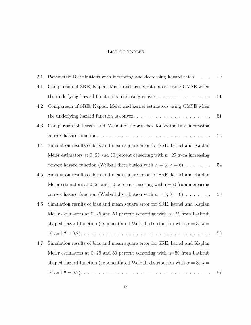
2.1 Parametric Distributions with increasing and decreasing hazard rates . . . . 9
4.1 Comparison of SRE, Kaplan Meier and kernel estimators using OMSE when
the underlying hazard function is increasing convex. . . . . . . . . . . . . . . 51
4.2 Comparison of SRE, Kaplan Meier and kernel estimators using OMSE when
the underlying hazard function is convex. . . . . . . . . . . . . . . . . . . . . 51
4.3 Comparison of Direct and Weighted approaches for estimating increasing
convex hazard function. . . . . . . . . . . . . . . . . . . . . . . . . . . . . . 53
4.4 Simulation results of bias and mean square error for SRE, kernel and Kaplan
Meier estimators at 0, 25 and 50 percent censoring with n=25 from increasing
convex hazard function (Weibull distribution with α = 3, λ = 6). . . . . . . . 54
4.5 Simulation results of bias and mean square error for SRE, kernel and Kaplan
Meier estimators at 0, 25 and 50 percent censoring with n=50 from increasing
convex hazard function (Weibull distribution with α = 3, λ = 6). . . . . . . . 55
4.6 Simulation results of bias and mean square error for SRE, kernel and Kaplan
Meier estimators at 0, 25 and 50 percent censoring with n=25 from bathtub
shaped hazard function (exponentiated Weibull distribution with α = 3, λ =
10 and θ = 0.2). . . . . . . . . . . . . . . . . . . . . . . . . . . . . . . . . . . 56
4.7 Simulation results of bias and mean square error for SRE, kernel and Kaplan
Meier estimators at 0, 25 and 50 percent censoring with n=50 from bathtub
shaped hazard function (exponentiated Weibull distribution with α = 3, λ =
10 and θ = 0.2). . . . . . . . . . . . . . . . . . . . . . . . . . . . . . . . . . . 57
ix
x
5.1 Power values for specific values of η, nominal level 0.05, and n =25, 50 and
100 based on log rank (LR), Kolmogorov’s goodness of fit (KS) at 0 and 25
level of censoring. . . . . . . . . . . . . . . . . . . . . . . . . . . . . . . . . . 73
5.2 Size-power comparison for shape constrained and unconstrained tests for spe-
cific values of η, nominal level 0.05 based on LR and KS without censoring. . 73
A.1 Survival times (in days) for patients in Arm A of the Head and Neck Cancer
Trial. The 0 denotes observations lost to follow up. . . . . . . . . . . . . . . 90
B.1 Bone Marrow Transplantation for acute lymphoblastic leukemia (ALL) group,
status=0 indicates alive or disease free, and status=1 indicates dead or relapsed.) 93
C.1 Data for Leukemia Patients, status=0 indicates still alive and status=1 indi-
cates dead. . . . . . . . . . . . . . . . . . . . . . . . . . . . . . . . . . . . . . 95
D.1 Generator fan failure data in thousands of hours of running time; status=1
indicates failure, and status=0 indicates censored. . . . . . . . . . . . . . . . 98
List of Figures
1.1 Typical Hazard Shapes. . . . . . . . . . . . . . . . . . . . . . . . . . . . . . 3
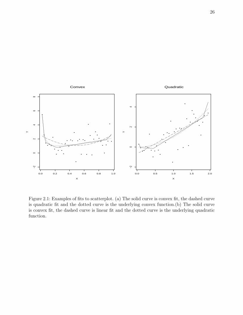
2.1 Examples of fits to scatterplot. (a) The solid curve is convex fit, the dashed
curve is quadratic fit and the dotted curve is the underlying convex func-
tion.(b) The solid curve is convex fit, the dashed curve is linear fit and the
dotted curve is the underlying quadratic function. . . . . . . . . . . . . . . . 26
3.1 Estimation results using percentiles as data. The failure times are quantiles of
exponentiated Weibull distribution with parameters α = 4, η = 1 and λ = 10.
The thin solid curve is the underlying hazard rate, the thick solid curve is
SRE estimate, the dotted curve is kernel estimate, and the dashed curve is
Kaplan Meier estimate. . . . . . . . . . . . . . . . . . . . . . . . . . . . . . . 41
3.2 Estimation results using percentiles as data. The failure times are quantiles
of exponentiated Weibull distribution with parameters α = 3, η = 0.2 and
λ = 10. The thin solid curve is the underlying hazard rate estimate, the
thick solid curve is SRE estimate, the dotted curve is kernel estimate, and the
dashed curve is Kaplan Meier estimate. . . . . . . . . . . . . . . . . . . . . . 42
3.3 Estimation results using percentiles as data. The failure times are quantiles
of a distribution function with quadratic hazard function. The thin curve is
the underlying hazard rate, the thick solid curve is SRE estimate, the dotted
curve is kernel estimate, and the dashed curve is Kaplan Meier estimate. . . 44
xi
xii
3.4 Comparison of Survival functions estimated by different methods. The thin
solid curve is the underlying survival function, the thick solid curve is the
shape restricted estimate, the dotted curve is Kaplan Meier estimate and the
dashed curve is kernel estimate. . . . . . . . . . . . . . . . . . . . . . . . . . 46
4.1 Estimates of hazard rates for the head and neck cancer data based on kernel
(dashed curve), SRE (solid curve) and parametric (dotted curve) estimators. 58
4.2 Estimates of hazard rates for the bone marrow transplantation data based
on SRE (thick solid curve), kernel (dashed curve) and PMLE (dotted curve)
estimators. . . . . . . . . . . . . . . . . . . . . . . . . . . . . . . . . . . . . . 59
4.3 Estimates of hazard rates for the Leukemia Survival Data based on SRE (solid
curve), kernel (dotted curve) and Kaplan Meier (short dashed curve) and
PMLE (long dashed curve) estimators. . . . . . . . . . . . . . . . . . . . . . 60
5.1 Graph of hazard function for the model (5.3.1) when α = 6, λ = 10 and η = 1,
0.75 and 0.5 (solid curves) from lowest to highest, η =0.025 and 0.01 (dashed
curves) from lowest to highest, and α = 1, η = 1 (dotted curve). . . . . . . . 70
5.2 Power at selected η values for nominal level 0.05, for log-rank test for 25 ( solid
curve), 50 (dotted curve) and 100 (short dashed curve) sample sizes, while the
long dashed curve represents the nominal level α = 0.05. . . . . . . . . . . . 74
6.1 The edges for convex piecewise quadratic when K=5, with equally spaced knots. 81
6.2 Comparison of SRE and quadratic spline, the failure times are generated from
Weibull distribution with shape and scale parameters 3 and 0.03. The dotted
curve is the underlying hazard rate, the dashed curve is SRE estimate and
the solid curve is shape restricted quadratic spline estimate. . . . . . . . . . 82
Chapter 1
INTRODUCTION
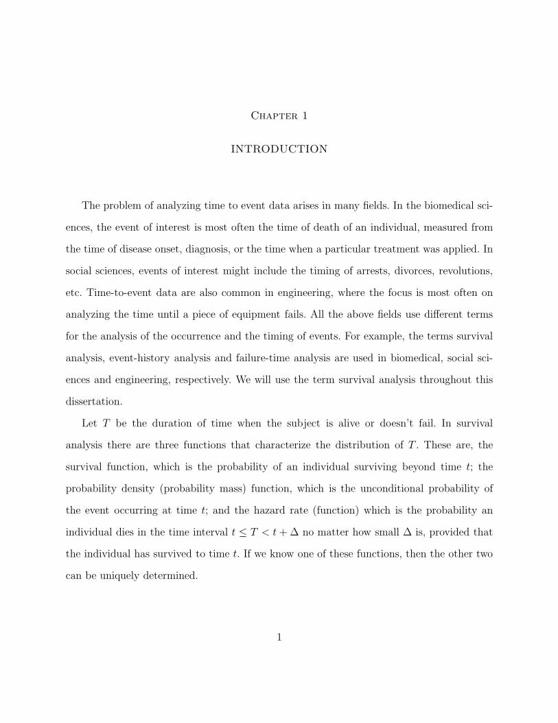
The problem of analyzing time to event data arises in many fields. In the biomedical sci-
ences, the event of interest is most often the time of death of an individual, measured from
the time of disease onset, diagnosis, or the time when a particular treatment was applied. In
social sciences, events of interest might include the timing of arrests, divorces, revolutions,
etc. Time-to-event data are also common in engineering, where the focus is most often on
analyzing the time until a piece of equipment fails. All the above fields use different terms
for the analysis of the occurrence and the timing of events. For example, the terms survival
analysis, event-history analysis and failure-time analysis are used in biomedical, social sci-
ences and engineering, respectively. We will use the term survival analysis throughout this
dissertation.
Let T be the duration of time when the subject is alive or doesn’t fail. In survival
analysis there are three functions that characterize the distribution of T . These are, the
survival function, which is the probability of an individual surviving beyond time t; the
probability density (probability mass) function, which is the unconditional probability of
the event occurring at time t; and the hazard rate (function) which is the probability an
individual dies in the time interval t ≤ T < t + ∆ no matter how small ∆ is, provided that
the individual has survived to time t. If we know one of these functions, then the other two
can be uniquely determined.
1
2
The hazard function is a fundamental quantity in survival analysis. It is also termed
as the failure rate, the instantaneous death rate, or the force of mortality and is defined
mathematically as,
h(t) = lim∆t→0
p(t ≤ T < t + ∆|T ≥ t)
∆t.
The hazard function is usually more informative about the underlying mechanism of
failure than the survival function. For this reason, modeling the hazard function is an impor-
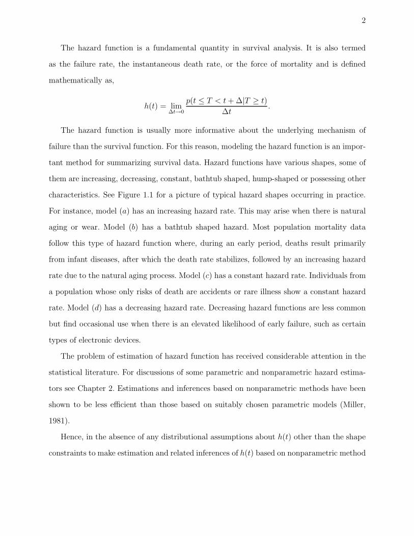
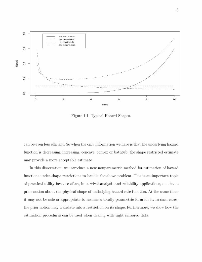
tant method for summarizing survival data. Hazard functions have various shapes, some of
them are increasing, decreasing, constant, bathtub shaped, hump-shaped or possessing other
characteristics. See Figure 1.1 for a picture of typical hazard shapes occurring in practice.
For instance, model (a) has an increasing hazard rate. This may arise when there is natural
aging or wear. Model (b) has a bathtub shaped hazard. Most population mortality data
follow this type of hazard function where, during an early period, deaths result primarily
from infant diseases, after which the death rate stabilizes, followed by an increasing hazard
rate due to the natural aging process. Model (c) has a constant hazard rate. Individuals from
a population whose only risks of death are accidents or rare illness show a constant hazard
rate. Model (d) has a decreasing hazard rate. Decreasing hazard functions are less common
but find occasional use when there is an elevated likelihood of early failure, such as certain
types of electronic devices.
The problem of estimation of hazard function has received considerable attention in the
statistical literature. For discussions of some parametric and nonparametric hazard estima-
tors see Chapter 2. Estimations and inferences based on nonparametric methods have been
shown to be less efficient than those based on suitably chosen parametric models (Miller,
1981).
Hence, in the absence of any distributional assumptions about h(t) other than the shape
constraints to make estimation and related inferences of h(t) based on nonparametric method
3
Time
Haza
rd
0 2 4 6 8 10
0.00.2
0.40.6
0.8
a) increaseb) constant b) bathtubd) decrease
Figure 1.1: Typical Hazard Shapes.
can be even less efficient. So when the only information we have is that the underlying hazard
function is decreasing, increasing, concave, convex or bathtub, the shape restricted estimate
may provide a more acceptable estimate.
In this dissertation, we introduce a new nonparametric method for estimation of hazard
functions under shape restrictions to handle the above problem. This is an important topic
of practical utility because often, in survival analysis and reliability applications, one has a
prior notion about the physical shape of underlying hazard rate function. At the same time,
it may not be safe or appropriate to assume a totally parametric form for it. In such cases,
the prior notion may translate into a restriction on its shape. Furthermore, we show how the
estimation procedures can be used when dealing with right censored data.
4
We also study the problem of testing whether survival times can be modeled by certain
parametric families which are often assumed in applications. Instead of omnibus tests, we
compare hazard rates derived nonparametrically but under similar shape restrictions as
the parametric hazard. We use appropriate resampling-based computation to conduct our
tests since the asymptotic distributions of the test statistics in these problems are largely
intractable.
Estimation and inference for tests involving shape restriction are not easy but methods
for their numerical computation exists (Robertson, Wright, and Dykstra 1988; Fraser and
Massam 1989; Meyer 1999a). We review this issue in detail in Chapter 2, section 2.4.
In our approach, we consider the maximum likelihood technique for estimating the con-
strained hazard function. The shape restricted estimator can be obtained through iteratively
reweighted least squares. This technique has been used in a variety of contexts. Meyer (1999b)
used iteratively reweighted least squares to estimate the maximum likelihood of constrained
potency curve. Meyer and Lund (2003) also applied this technique on time series data for
estimating shape restricted trend models. In addition, Fraser and Massam (1989) applied
the weighted least squares method to obtain the least square estimate of concave regression.
The problem of finding the least square estimator of the concave and convex function
over the constraint space is a quadratic programming problem. There is no known closed
form solution, but it can be obtained by the hinge algorithm of Meyer (1999) or the mixed
primal-dual bases algorithm of Fraser and Massam (1989). These algorithms are given in
section 2.4.
The dissertation is organized as follows: In Chapter 2 we begin with a review of the
literature. We discuss various estimation methods proposed for the hazard rate. This Chapter
also presents a summary review of shape restricted regression and the constraint cone, over
which we maximize the likelihood or minimize the sum of squared errors. In Chapter 3, the
general formulation and some theoretical properties of our method are discussed. Section

5
3.1 deals with construction of the new estimator for uncensored data and section 3.2 deals
with the problem of estimation of hazard function for right censored data. For the right
censored data case, two approaches of obtaining the shape restricted estimator for hazard
are discussed. Simulation results and some real examples are given in Chapter 4. Chapter 5 is
devoted to testing for shape restricted hazard function using resampling technique. Finally,
Chapter 6 deals with future research:
1. Bayesian approaches to the shape restricted hazard function,
2. Marginal estimation of hazard function under shape restriction in presence of depen-
dent censoring, and
3. Hazard function estimation using splines under shape restrictions.

Chapter 2
LITERATURE REVIEW
In this chapter we give basic definitions of functions related to lifetimes. We also review
some pre-existing methods used in the estimation of the hazard function and provide some
background of shape restricted regression.
2.1 Distribution of failure time
Let T denote a nonnegative random variable representing the lifetime of an individual in
some population. Suppose that the lifetime T has the distribution function F and density
f . We would then define the survival function of T as
S(t) = P (T > t) = 1 − F (t).
If T is a continuous random variable, then
h(t) =f(t)
S(t)= lim
∆t→0
p(t ≤ T < t + ∆|T ≥ t)
∆t.
A related quantity is the cumulative hazard function H(t), defined by
H(t) =∫ t
0h(u)du = − log(S(t)).
Thus, for continuous lifetimes we have the following relationships:
1. S(t) = exp(−H(t)) = exp−∫ t0 h(u)du;
2. h(t) = −log S(t)′;
6
7
3. f(t) = −S ′(t);
4. f(t) = h(t) exp−H(t).
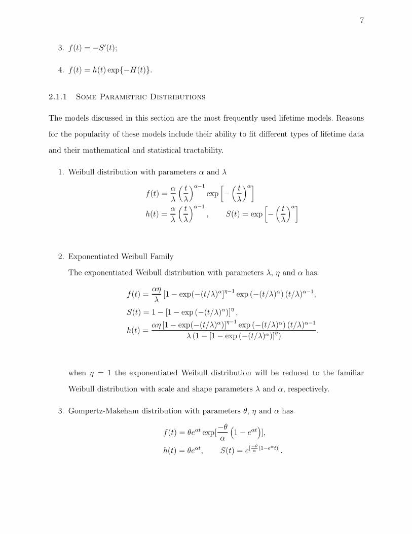
2.1.1 Some Parametric Distributions
The models discussed in this section are the most frequently used lifetime models. Reasons
for the popularity of these models include their ability to fit different types of lifetime data
and their mathematical and statistical tractability.
1. Weibull distribution with parameters α and λ
f(t) =α
λ
(
t
λ
)α−1
exp[
−(
t
λ
)α]
h(t) =α
λ
(
t
λ
)α−1
, S(t) = exp[
−(
t
λ
)α]
2. Exponentiated Weibull Family
The exponentiated Weibull distribution with parameters λ, η and α has:
f(t) =αη
λ[1 − exp(−(t/λ)α]η−1 exp (−(t/λ)α) (t/λ)α−1,
S(t) = 1 − [1 − exp (−(t/λ)α)]η ,
h(t) =αη [1 − exp(−(t/λ)α)]η−1 exp (−(t/λ)α) (t/λ)α−1
λ (1 − [1 − exp (−(t/λ)α)]η).
when η = 1 the exponentiated Weibull distribution will be reduced to the familiar
Weibull distribution with scale and shape parameters λ and α, respectively.
3. Gompertz-Makeham distribution with parameters θ, η and α has
f(t) = θeαt exp[−θ
α
(
1 − eαt)
],
h(t) = θeαt, S(t) = e[−θα
(1−eαt)].
8
4. Rayleigh distribution with parameters λ0, and λ1 has
f(t) = (λ0 + λ1t) exp(
−λ0t − 0.5λ1t2)
h(t) = λ0 + λ1t, S(t) = exp(
−λ0t − 0.5λ1t2)
.
5. Pareto distribution with parameters λ, and α has
f(t) =θλθ
tθ+1,
h(t) =θ
t, S(t) =
λθ
tθ.
From the different models we can see that hazard functions can be quite different in functional
form. It is hard to choose the appropriate model from these different parametric models of
no theoretical basis. In the absence of any strong distributional assumptions about h(·) other
than its shape, it may not be appropriate to use a totally parametric form of the hazard func-
tion. For example, the concepts of a distribution functions with increasing hazard function
are useful in engineering applications (Miller, 1981). However, we have many distributions
that have an increasing hazard function; this makes it difficult to select one without an
appropriate theoretical basis (see the Table 2.1). In addition to that, these models are not
capable of giving different shapes of hazard function such as U-shape hazard function, and
bimodal hazard function. For such conditions when the only information available is the
shape (decreasing, increasing, concave, convex or bathtub) of the underlying hazard func-
tion, a new nonparametric estimator that considers shape is introduced in this dissertation
to provide more acceptable estimates.
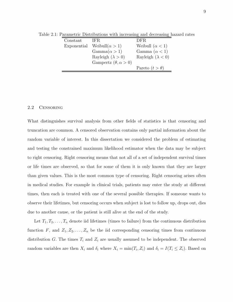
In Table 2.1 IFR and DFR stands for an increasing hazard rate and a decreasing hazard
rate, respectively.
9
Table 2.1: Parametric Distributions with increasing and decreasing hazard rates
Constant IFR DFRExponential Weibull(α > 1) Weibull (α < 1)
Gamma(α > 1) Gamma (α < 1)Rayleigh (λ > 0) Rayleigh (λ < 0)Gampertz (θ, α > 0)
Pareto (t > θ)
2.2 Censoring
What distinguishes survival analysis from other fields of statistics is that censoring and
truncation are common. A censored observation contains only partial information about the
random variable of interest. In this dissertation we considered the problem of estimating
and testing the constrained maximum likelihood estimator when the data may be subject
to right censoring. Right censoring means that not all of a set of independent survival times
or life times are observed, so that for some of them it is only known that they are larger
than given values. This is the most common type of censoring. Right censoring arises often
in medical studies. For example in clinical trials, patients may enter the study at different
times, then each is treated with one of the several possible therapies. If someone wants to
observe their lifetimes, but censoring occurs when subject is lost to follow up, drops out, dies
due to another cause, or the patient is still alive at the end of the study.
Let T1, T2, . . . , Tn denote iid lifetimes (times to failure) from the continuous distribution
function F , and Z1, Z2, . . . , Zn be the iid corresponding censoring times from continuous
distribution G. The times Ti and Zi are usually assumed to be independent. The observed
random variables are then Xi and δi where Xi = min(Ti, Zi) and δi = I(Ti ≤ Zi). Based on

10
this assumption and the distribution of Z does not involve any parameters of interest, we
derived the maximum likelihood function of the lifetimes in the next section.
2.3 Estimation
2.3.1 Parametric Procedures
Parametric methods rest on the assumption that h(t) is a member of some family of dis-
tributions h(t, θ), where h is known but depends on an unknown parameter θ, possibly
vector-valued. In general, θ is estimated in some optimal fashion, and its estimator θ is used
in h(t, θ) to obtain a parametric estimator of h(t) (Lawless, 1982; Miller, 1981). The Weibull
distribution is considered as illustrative of the parametric approach. Because of its flexibility
the Weibull distribution has been widely used as a model in fitting lifetimes data. Various
problems associated with this distribution have been considered by Cohen (1965) and many
other authors.
The likelihood function:
Here we concentrate on methods based on the likelihood function for a right censored sample.
We derive the general form of the likelihood function. Let T denote a lifetime with distribu-
tion function F , probability density function (pdf) f and survival function Sf ; and Z denote
a random censoring time with distribution function G, pdf g, and survival function Sg.
The derivation of the likelihood is as follows:
P (X = x, δ = 0) = P (Z = x, Z < T ) = P (Z = x, x < T )
= P (Z = x)P (x < T ) = g(x)Sf(x) by independence
P (X = x, δ = 1) = P (T = x, T < Z)
= P (T = x, x < Z) = f(x)Sg(x) by independence
11
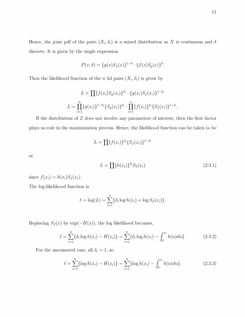
Hence, the joint pdf of the pairs (Xi, δi) is a mixed distribution as X is continuous and δ
discrete. It is given by the single expression
P (x, δ) = g(x)Sf(x)1−δ · f(x)Sg(x)δ.
Then the likelihood function of the n iid pairs (Xi, δi) is given by
L =∏
f(xi)Sg(xi)δi · g(xi)Sf(xi)
1−δi
L =n∏
i=1
g(xi)1−δiSg(xi)
δi ·n∏
i=1
f(xi)δiSf(xi)
1−δi .
If the distribution of Z does not involve any parameters of interest, then the first factor
plays no role in the maximization process. Hence, the likelihood function can be taken to be
L =∏
f(xi)δiSf (xi)
1−δi
or
L =∏
h(xi)δiSf(xi) (2.3.1)
since f(xi) = h(xi)Sf(xi).
The log-likelihood function is
ℓ = log(L) =n∑
i=1
δi log h(xi) + log Sf (xi).
Replacing Sf (x) by exp(−H(x)), the log likelihood becomes,
ℓ =n∑
i=1
δi log h(xi) − H(xi) =n∑
i=1
δi log h(xi) −∫ xi
0h(u)du. (2.3.2)
For the uncensored case, all δi = 1, so
ℓ =n∑
i=1
log h(xi) − H(xi) =n∑
i=1
log h(xi) −∫ xi
0h(u)du. (2.3.3)
12
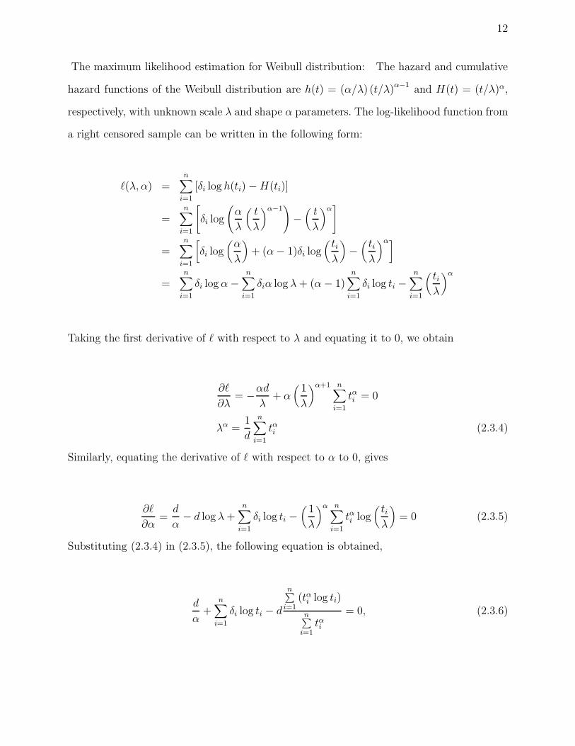
The maximum likelihood estimation for Weibull distribution: The hazard and cumulative
hazard functions of the Weibull distribution are h(t) = (α/λ) (t/λ)α−1 and H(t) = (t/λ)α,
respectively, with unknown scale λ and shape α parameters. The log-likelihood function from
a right censored sample can be written in the following form:
ℓ(λ, α) =n∑
i=1
[δi log h(ti) − H(ti)]
=n∑
i=1
[
δi log
(
α
λ
(
t
λ
)α−1)
−(
t
λ
)α]
=n∑
i=1
[
δi log(
α
λ
)
+ (α − 1)δi log(
tiλ
)
−(
tiλ
)α]
=n∑
i=1
δi log α −n∑
i=1
δiα log λ + (α − 1)n∑
i=1
δi log ti −n∑
i=1
(
tiλ
)α
Taking the first derivative of ℓ with respect to λ and equating it to 0, we obtain
∂ℓ
∂λ= −
αd
λ+ α
(
1
λ
)α+1 n∑
i=1
tαi = 0
λα =1
d
n∑
i=1
tαi (2.3.4)
Similarly, equating the derivative of ℓ with respect to α to 0, gives
∂ℓ
∂α=
d
α− d log λ +
n∑
i=1
δi log ti −(
1
λ
)α n∑
i=1
tαi log(
tiλ
)
= 0 (2.3.5)
Substituting (2.3.4) in (2.3.5), the following equation is obtained,
d
α+
n∑
i=1
δi log ti − d
n∑
i=1(tαi log ti)
n∑
i=1tαi
= 0, (2.3.6)
13
where d is the number of uncensored values.
If the shape parameter α is known, then the maximum likelihood estimator (MLE) of λ
can be obtained explicitly using (2.3.4). However, if α is unknown, then we cannot have an
explicit form of the MLE. Equation (2.3.6) can be solved for α using the Newton-Raphson
iterative method. Then the associated estimator of h(α, λ) is h(α, λ), where α, λ are the
MLEs of α, λ, respectively.
2.3.2 Nonparametric Procedures
Nonparametric procedures, on the other hand, do not require any distributional assumptions
about h(t). Thus, they are more flexible than their parametric counterparts, and as a result
they are widely used in the analysis of failure times (Kouassi and Singh, 1997). For discus-
sions of some nonparametric hazard estimators see Aalen (1978); Cox (1972); Watson and
Leadbetter (1964b); Antoniadis et al. (1999); Liu and Van Ryzin (1984); Ramlau-Hansen
(1983); and Kouassi and Singh (1997). For the present discussion we next review several of
these nonparametric approaches:
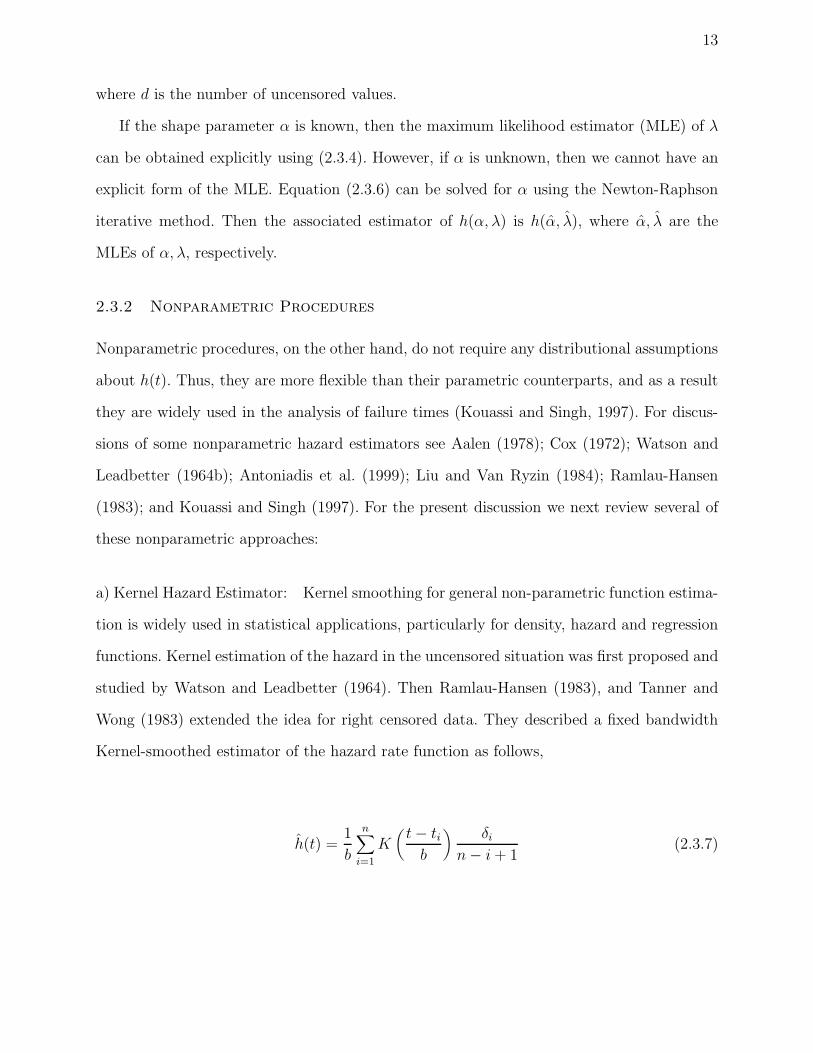
a) Kernel Hazard Estimator: Kernel smoothing for general non-parametric function estima-
tion is widely used in statistical applications, particularly for density, hazard and regression
functions. Kernel estimation of the hazard in the uncensored situation was first proposed and
studied by Watson and Leadbetter (1964). Then Ramlau-Hansen (1983), and Tanner and
Wong (1983) extended the idea for right censored data. They described a fixed bandwidth
Kernel-smoothed estimator of the hazard rate function as follows,
h(t) =1
b
n∑
i=1
K(
t − tib
)
δi
n − i + 1(2.3.7)
14
where K(·) is a kernel function, b is the bandwidth which determines the degree of smooth-
ness. In this dissertation the Epanechnikov kernel K(x) = 0.75(1 − x2) for −1 ≤ x ≤ 1 was
used throughout the examples and simulation studies.
b) Kaplan-Meier Type Estimate: Smith (2002), among many authors, discuss the following
estimates of the hazard function. Let ti denote a distinct ordered death time, i = 1, . . . , r ≤ n,
then the hazard rate function is estimated by h(ti) = di/ni and h(t) = di/ni(ti+1 − ti) at
an observed death ti and in the interval ti ≤ t < ti+1, respectively. Here di is the number of
deaths at ith death time and ni is the number of individuals at risk of death at time ti.
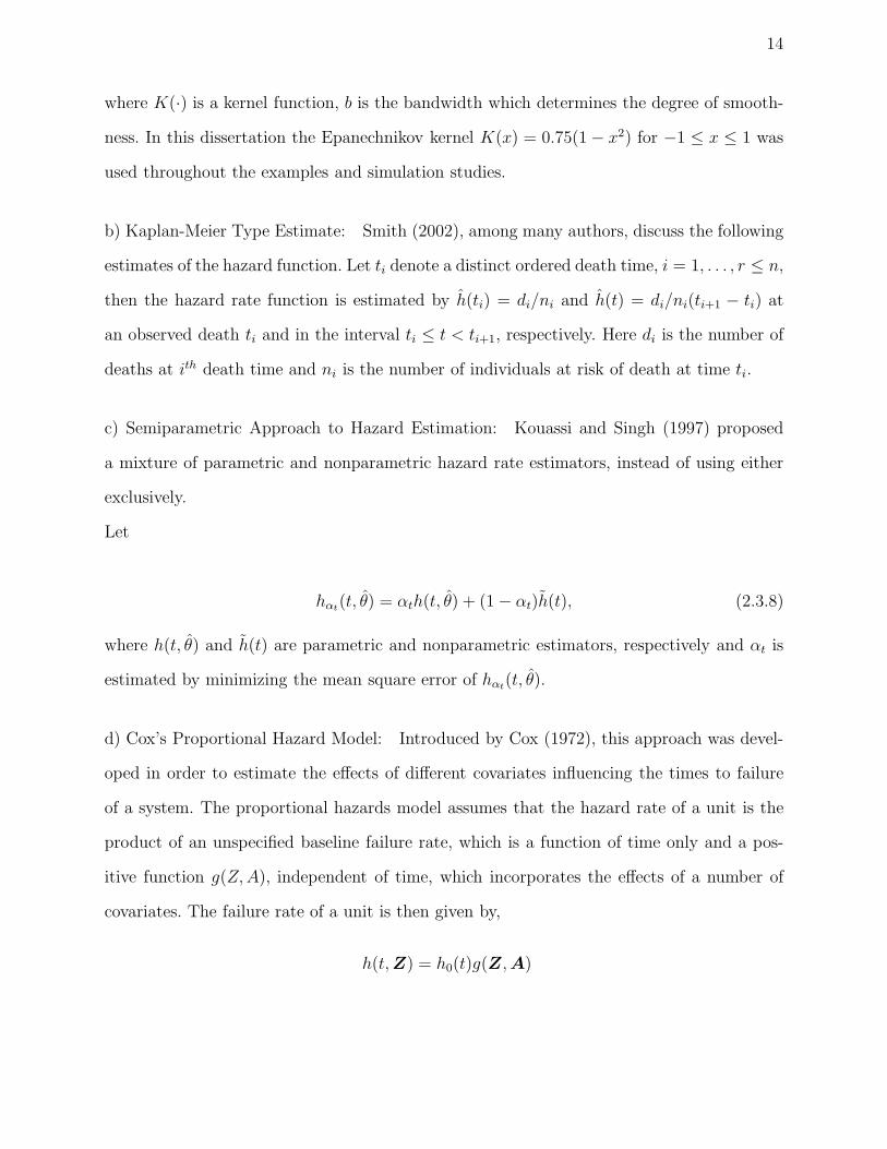
c) Semiparametric Approach to Hazard Estimation: Kouassi and Singh (1997) proposed
a mixture of parametric and nonparametric hazard rate estimators, instead of using either
exclusively.
Let
hαt(t, θ) = αth(t, θ) + (1 − αt)h(t), (2.3.8)
where h(t, θ) and h(t) are parametric and nonparametric estimators, respectively and αt is
estimated by minimizing the mean square error of hαt(t, θ).
d) Cox’s Proportional Hazard Model: Introduced by Cox (1972), this approach was devel-
oped in order to estimate the effects of different covariates influencing the times to failure
of a system. The proportional hazards model assumes that the hazard rate of a unit is the
product of an unspecified baseline failure rate, which is a function of time only and a pos-
itive function g(Z, A), independent of time, which incorporates the effects of a number of
covariates. The failure rate of a unit is then given by,
h(t, Z) = h0(t)g(Z, A)
15
where h0 is the baseline hazard rate, Z is a row vector consisting of the covariates, A is a
column vector consisting of the unknown parameters (also called regression parameters) of
the model. It can be assumed that the form of g(Z, A) is known and t is unspecified.
2.4 Shape Restricted Regression
In this section before we introduce our new nonparametric shape restricted estimator, we
review some fundamental concepts that can help us to lay groundwork for the construction
of the shape restricted estimator. The definitions, results, and their proofs along with more
details about the properties of the constraint cone and polar cones can be found in Rockafellar
(1970), Robertson et al. (1988), Fraser and Massam (1989), and Meyer (1999a).
Suppose we have the following model
yi = f(xi) + σǫi, i = 1, · · · , n.
In this model the errors ǫi’s are independent and have standard normal distribution, f ∈ Λ,
and Λ is a class of regression functions sharing a qualitative property such as monotonicity,
convexity or concavity.
The constrained set over which we maximize the likelihood or minimize the sum of squared
errors is constructed as follows: let θi = f(xi) and xi’s are known, distinct and ordered for
1 ≤ i ≤ n. The monotone nondecreasing constraints can be written as
θ1 ≤ θ2 ≤ . . . ≤ θn
If we consider piecewise linear approximations to the regression function with knots at
x−values, the nondecreasing convex, nondecreasing concave and convex shape restrictions
can be written as a set of linear inequality constraints. For example, if we are considering
convex, then we have
16
θ2 − θ1
x2 − x1≤
θ3 − θ2
x3 − x2≤ . . . ≤
θn − θn−1
xn − xn−1.
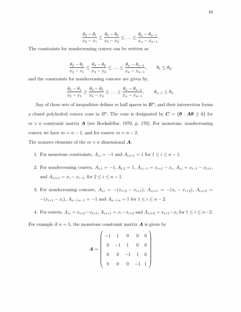
The constraints for nondecreasing convex can be written as
θ2 − θ1
x2 − x1
≤θ3 − θ2
x3 − x2
≤ . . . ≤θn − θn−1
xn − xn−1
, θ1 ≤ θ2,
and the constraints for nondecreasing concave are given by,
θ2 − θ1
x2 − x1≥
θ3 − θ2
x3 − x2≥ . . . ≥
θn − θn−1
xn − xn−1, θn−1 ≤ θn.
Any of these sets of inequalities defines m half spaces in IRn, and their intersection forms
a closed polyhedral convex cone in Rn. The cone is designated by C = θ : Aθ ≥ 0 for
m × n constraint matrix A (see Rockafellar, 1970, p. 170). For monotone, nondecreasing
convex we have m = n − 1, and for convex m = n − 2.
The nonzero elements of the m × n dimensional A:
1. For monotone constraints, Ai,i = −1 and Ai,i+1 = 1 for 1 ≤ i ≤ n − 1.
2. For nondecreasing convex, A1,1 = −1, A1,2 = 1, Ai,i−1 = xi+1 − xi, Ai,i = xi−1 − xi+1,
and Ai,i+1 = xi − xi−1, for 2 ≤ i ≤ n − 1.
3. For nondecreasing concave, Ai,i = −(xi+2 − xi+1), Ai,i+1 = −(xi − xi+2), Ai,i+2 =
−(xi+1 − xi), An−1,n−1 = −1 and An−1,n = 1 for 1 ≤ i ≤ n − 2.
4. For convex, Ai,i = xi+2−xi+1, Ai,i+1 = xi−xi+2 and Ai,i+2 = xi+1−xi for 1 ≤ i ≤ n−2.
For example if n = 5, the monotone constraint matrix A is given by
A =
−1 1 0 0 0
0 −1 1 0 0
0 0 −1 1 0
0 0 0 −1 1
17
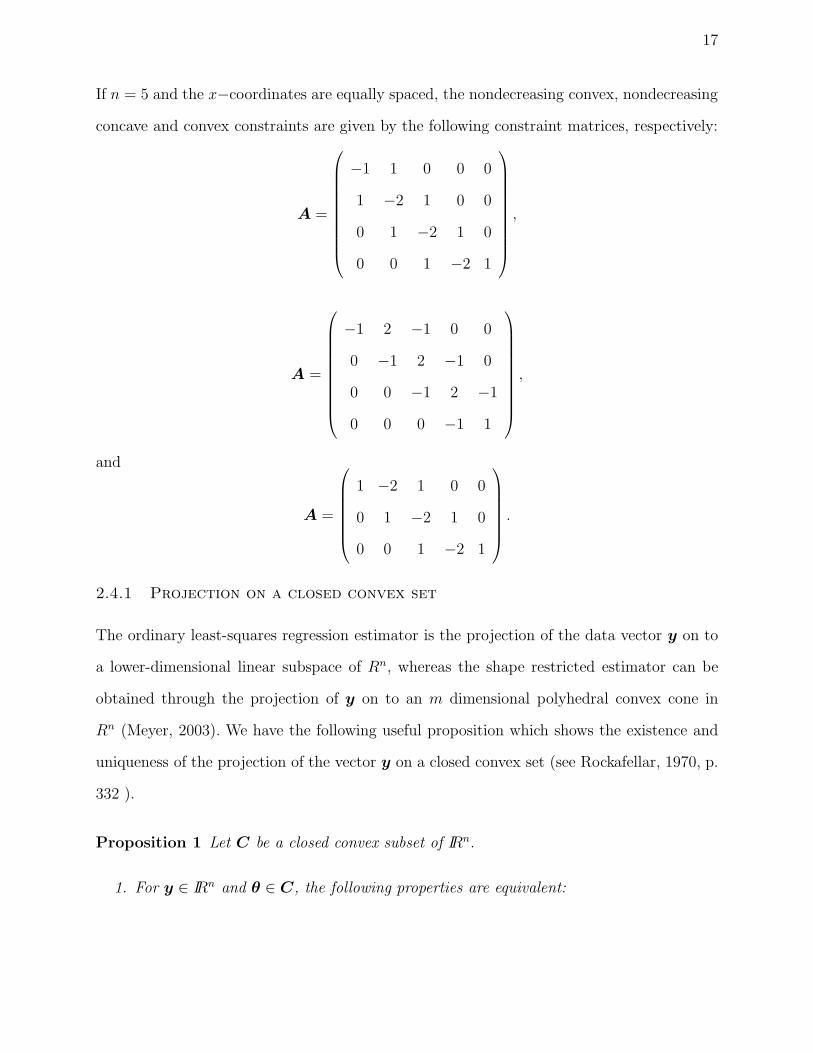
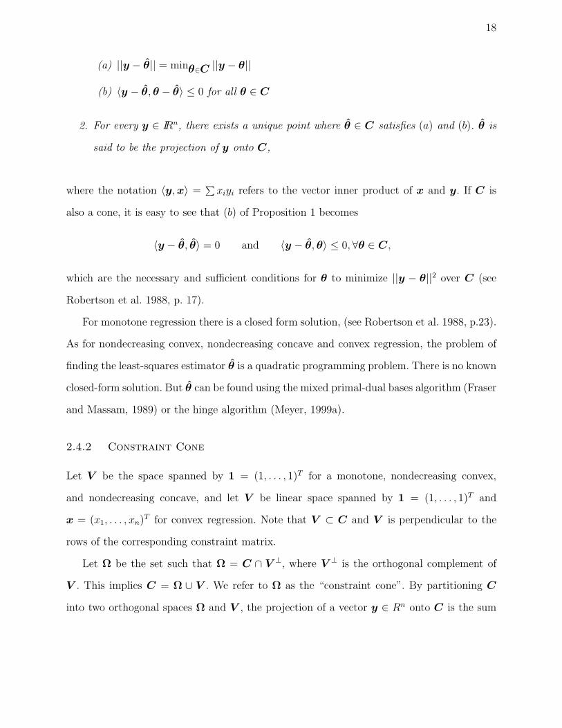
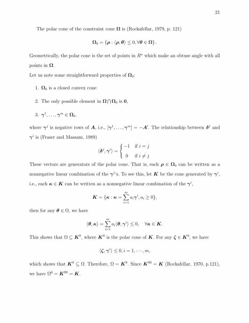
If n = 5 and the x−coordinates are equally spaced, the nondecreasing convex, nondecreasing
concave and convex constraints are given by the following constraint matrices, respectively:
A =
−1 1 0 0 0
1 −2 1 0 0
0 1 −2 1 0
0 0 1 −2 1
,
A =
−1 2 −1 0 0
0 −1 2 −1 0
0 0 −1 2 −1
0 0 0 −1 1
,
and
A =
1 −2 1 0 0
0 1 −2 1 0
0 0 1 −2 1
.
2.4.1 Projection on a closed convex set
The ordinary least-squares regression estimator is the projection of the data vector y on to
a lower-dimensional linear subspace of Rn, whereas the shape restricted estimator can be
obtained through the projection of y on to an m dimensional polyhedral convex cone in
Rn (Meyer, 2003). We have the following useful proposition which shows the existence and
uniqueness of the projection of the vector y on a closed convex set (see Rockafellar, 1970, p.
332 ).
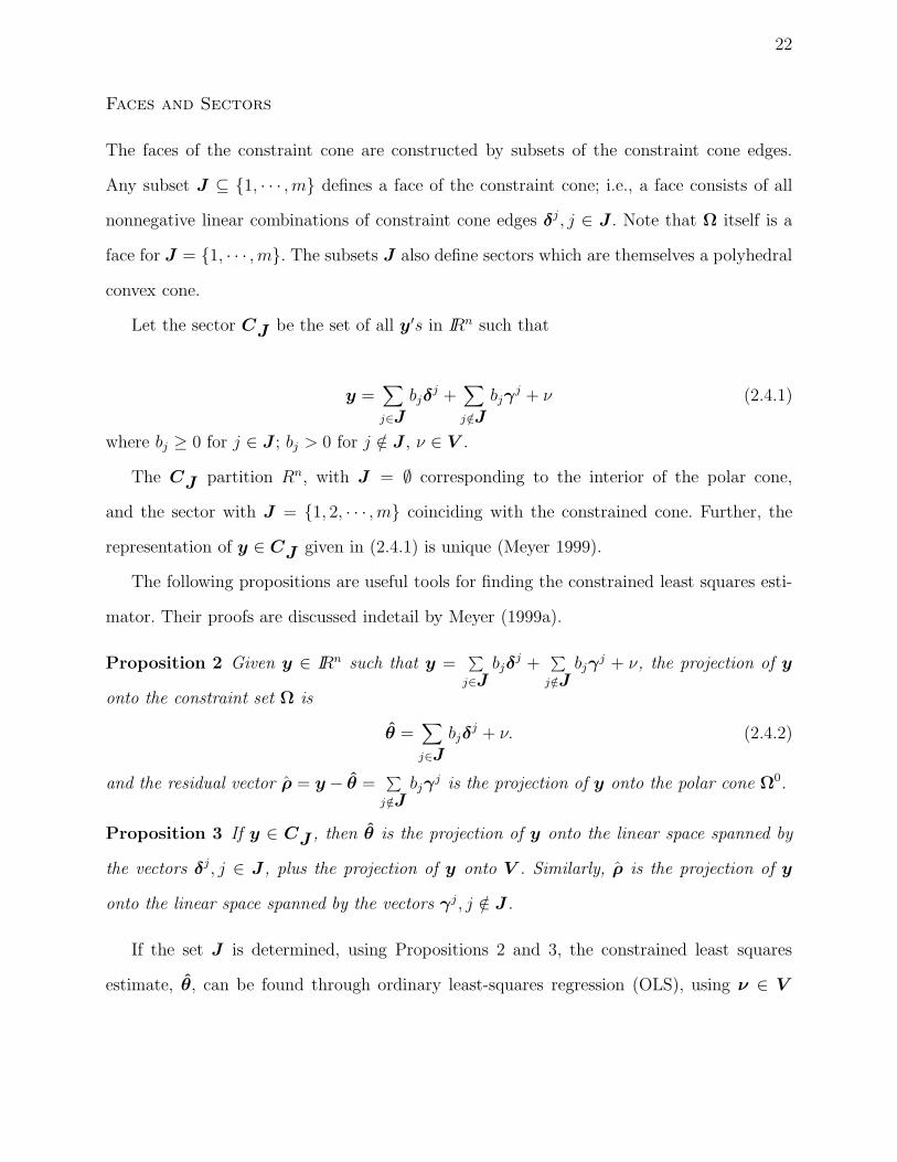
Proposition 1 Let C be a closed convex subset of IRn.
1. For y ∈ IRn and θ ∈ C, the following properties are equivalent:
18
(a) ||y − θ|| = minθ∈C ||y − θ||
(b) 〈y − θ, θ − θ〉 ≤ 0 for all θ ∈ C
2. For every y ∈ IRn, there exists a unique point where θ ∈ C satisfies (a) and (b). θ is
said to be the projection of y onto C,
where the notation 〈y, x〉 =∑
xiyi refers to the vector inner product of x and y. If C is
also a cone, it is easy to see that (b) of Proposition 1 becomes
〈y − θ, θ〉 = 0 and 〈y − θ, θ〉 ≤ 0, ∀θ ∈ C,
which are the necessary and sufficient conditions for θ to minimize ||y − θ||2 over C (see
Robertson et al. 1988, p. 17).
For monotone regression there is a closed form solution, (see Robertson et al. 1988, p.23).
As for nondecreasing convex, nondecreasing concave and convex regression, the problem of
finding the least-squares estimator θ is a quadratic programming problem. There is no known
closed-form solution. But θ can be found using the mixed primal-dual bases algorithm (Fraser
and Massam, 1989) or the hinge algorithm (Meyer, 1999a).
2.4.2 Constraint Cone
Let V be the space spanned by 1 = (1, . . . , 1)T for a monotone, nondecreasing convex,
and nondecreasing concave, and let V be linear space spanned by 1 = (1, . . . , 1)T and
x = (x1, . . . , xn)T for convex regression. Note that V ⊂ C and V is perpendicular to the
rows of the corresponding constraint matrix.
Let Ω be the set such that Ω = C ∩ V ⊥, where V ⊥ is the orthogonal complement of
V . This implies C = Ω ∪ V . We refer to Ω as the “constraint cone”. By partitioning C
into two orthogonal spaces Ω and V , the projection of a vector y ∈ Rn onto C is the sum

19
of the projection of y onto Ω and V , which simplifies the computation. Besides, the edges
of Ω are unique up to multiplicative factor. The edges are a set of vectors in the constraint
cone such that any vector in Ω can be written as nonnegative linear combination of edges,
and no edge is itself a nonnegative linear combination of other edges. For a more detailed
discussion, see Meyer (1999) or Fraser and Massam (1989).
2.4.3 Edges of constraint cone and Polar cone
The constraint space can be specified by a set of linearly independent vectors δ1, . . . , δm.
So that Ω = θ : θ =∑m
j=1 bjδj : b1, . . . , bm ≥ 0 and the constraint set C = θ : θ =
∑mj=1 bjδ
j + ν : b1, . . . , bm, bj ≥ 0 and ν ∈ V , where m = n − 1 for monotone,
nondecreasing concave, nondecreasing convex and m = n − 2 for convex.
For example, if Ω is the set of all nondecreasing concave, nondecreasing convex, or convex
vectors in IRn, it can be specified using the vectors δj . The vectors δj can be obtained from
the formula ∆′ = (AA′)−1A = [δ1, . . . , δm]′.
For n = 5 and equally spaced x values , ∆′ is given by:
for convex,
∆′ =
2 −2 −1 0 1
4 −1 −6 −1 4
1 0 −1 −2 2
,
nondecreasing convex,
∆′ =
−10 −5 0 5 10
−6 −6 −1 4 9
−3 −3 −3 2 7
−1 −1 −1 −1 4
,
nondecreasing concave,

20
∆′ =
−4 1 1 1 1
−7 −2 3 3 3
−9 −4 1 6 6
−10 −5 0 5 10
,
and monotone
∆′ =
−4 1 1 1 1
−3 −3 2 2 2
−2 −2 −2 3 3
−1 −1 −1 −1 4
.
For convenience of presentation, the smallest possible multiplicative factors are chosen so that
all entries of ∆ are integers. Any convex vector θ ∈ C is a nonnegative linear combination
of the columns of the corresponding ∆ plus a linear combination of 1 and x.
If C is the set of all convex vectors in IRn we can also define the vectors δj to be the
rows of the following matrix:
0 0 x3−x2
xn−x2· · · · · · xn−1−x2
xn−x21
0 0 0 x4−x3
xn−x3· · · xn−1−x3
xn−x31
......
......
......
0 · · · · · · · · · · · · 0 1
1 · · · · · · · · · · · · 1 1
x1 · · · · · · · · · · · · xn−1 xn
For a large data set it is better to use the above vectors δj because the previous method of
obtaining the edges is computationally intensive. Another advantage is that the computations
of the inner products with the second approach are faster because of all the zero entries in
the vectors.
21
The polar cone of the constraint cone Ω is (Rockafellar, 1979, p. 121)
Ω0 = ρ : 〈ρ, θ〉 ≤ 0, ∀θ ∈ Ω .
Geometrically, the polar cone is the set of points in Rn which make an obtuse angle with all
points in Ω.
Let us note some straightforward properties of Ω0:
1. Ω0 is a closed convex cone
2. The only possible element in Ω⋂
Ω0 is 0,
3. γ1, . . . , γm ∈ Ω0.
where γj is negative rows of A, i.e., [γ1, . . . , γm] = −A′. The relationship between δj and
γi is (Fraser and Massam, 1989)
〈δj , γi〉 =
−1 if i = j
0 if i 6= j
These vectors are generators of the polar cone. That is, each ρ ∈ Ω0 can be written as a
nonnegative linear combination of the γj’s. To see this, let K be the cone generated by γi,
i.e., each κ ∈ K can be written as a nonnegative linear combination of the γi,
K = κ : κ =m∑
i=1
aiγi, ai ≥ 0,
then for any θ ∈ Ω, we have
〈θ, κ〉 =m∑
i=1
ai〈θ, γi〉 ≤ 0, ∀κ ∈ K.
This shows that Ω ⊆ K0, where K0 is the polar cone of K. For any ζ ∈ K0, we have
〈ζ, γi〉 ≤ 0, i = 1, · · · , m,
which shows that K0 ⊆ Ω. Therefore, Ω = K0. Since K00 = K (Rockafellar, 1970, p.121),
we have Ω0 = K00 = K.
22
Faces and Sectors
The faces of the constraint cone are constructed by subsets of the constraint cone edges.
Any subset J ⊆ 1, · · · , m defines a face of the constraint cone; i.e., a face consists of all
nonnegative linear combinations of constraint cone edges δj , j ∈ J . Note that Ω itself is a
face for J = 1, · · · , m. The subsets J also define sectors which are themselves a polyhedral
convex cone.
Let the sector CJ be the set of all y′s in IRn such that
y =∑
j∈J
bjδj +
∑
j /∈J
bjγj + ν (2.4.1)
where bj ≥ 0 for j ∈ J ; bj > 0 for j /∈ J , ν ∈ V .
The CJ partition Rn, with J = ∅ corresponding to the interior of the polar cone,
and the sector with J = 1, 2, · · · , m coinciding with the constrained cone. Further, the
representation of y ∈ CJ given in (2.4.1) is unique (Meyer 1999).
The following propositions are useful tools for finding the constrained least squares esti-
mator. Their proofs are discussed indetail by Meyer (1999a).
Proposition 2 Given y ∈ IRn such that y =∑
j∈Jbjδ
j +∑
j /∈Jbjγ
j + ν, the projection of y
onto the constraint set Ω is
θ =∑
j∈J
bjδj + ν. (2.4.2)
and the residual vector ρ = y − θ =∑
j /∈Jbjγ
j is the projection of y onto the polar cone Ω0.
Proposition 3 If y ∈ CJ , then θ is the projection of y onto the linear space spanned by
the vectors δj, j ∈ J , plus the projection of y onto V . Similarly, ρ is the projection of y
onto the linear space spanned by the vectors γj , j /∈ J .
If the set J is determined, using Propositions 2 and 3, the constrained least squares
estimate, θ, can be found through ordinary least-squares regression (OLS), using ν ∈ V
23
and δj for j ∈ J as regressors. Alternatively, ρ can be obtained through OLS using γj, for
j /∈ J as regressors, then θ = y − ρ. To find the set J and θ, Fraser and Massam (1989),
and Meyer (1999) proposed the mixed primal-dual bases algorithm and the hinge algorithm,
respectively. The method chosen in this paper is the hinge algorithm for it is fast, useful for
iterative projection algorithm and computationally more efficient.
2.4.4 The hinge algorithm
This algorithm uses a set of vectors δ1, · · · , δm and ν to characterize the constraint space.
The algorithm finds θ by finding J through a series of guesses Jk. At a typical iteration,
the current estimate θk can be obtained by the least-squares regression of y on the δj , for
j ∈ Jk and ν. We call δj the “hinges” since for the convex regression problem, the points
(xj , θj), j ∈ J , are the bending points at which the line segments change slope, and there is
only one way that the bends are allowed to go. The initial guess J0 is set to be empty.
The algorithm can be summarized in four steps:
1. Using ν as regressors to obtain a least-squares estimate θ0, for a convex, ν = 1, x
and for monotone, nondecreasing convex and nondecreasing concave, ν = 1.
Loop
2. At the kth iteration, compute 〈y−θk, δj〉 for each j /∈ Jk. If these are all non-positive,
then stop. If not, then add the vector δj to the model for which this inner product is
largest.
3. Get the least-squares fit with the new set of δ-vectors.
4. Check to see if the regression function satisfies the constraints on the coefficients, i.e.
is bj ≥ 0, for j ∈ J and j /∈ J0
24
. If yes, go to step 2.
. If no, choose the hinge with the largest negative coefficient and remove it from
the current set J . Go to step 3.
At each stage, the new hinge is added where it is “most needed”, and other hinges are
removed if the new fit does not satisfy the constraints. It is clear that if the algorithm ends,
it gives the correct solution and the algorithm does end. See Meyer (1999) for proof.
2.4.5 The mixed primal-dual bases algorithm
The mixed primal-dual bases algorithm is used to find the projection onto a closed convex
cone. In this algorithm, the γj ’s are the primal vectors and δj ’s are the dual vectors. The
mixed primal-dual bases algorithm finds the correct set J by moving along a line segment
connecting the point z0 =m∑
j=1δj with z, where z is the projection of the data y on the
subspace spanned by δj, j = 1, · · · , m. At the kth iteration, the point zk on the line segment
is reached, such that the distance between zk and z is strictly decreasing in k. This point is
also on a face of ΩJk. The next iteration finds zk+1 farther along the segment, on a face of
ΩJk+1. At the beginning of the iteration, both z and zk are expressed in the basis defined
by Jk, such as
z =∑
j∈Jk
bjδj +
∑
j /∈J k
bjγj ,
and
zk =∑
j∈J k
ajδj +
∑
j /∈J k
ajγj ,
where aj ≥ 0 for j ∈ Jk and aj > 0 for j /∈ Jk. If bj ≥ 0 for j ∈ Jk and bj > 0 for j /∈ Jk, the
algorithm stops. Otherwise, find
zk+1 = zk + αk+1(z − zk),
25
where αk+1 ∈ (0, 1) is as large as possible while the coefficients of zk+1 are all positive or
nonnegative as they are in Jk or not, respectively. The point zk+1 is on the face of ΩJ k,
which divides ΩJkand ΩJk+1
. The algorithm terminates at the face of the sector containing
z. It clearly takes a finite number of iterations since there are a finite number of sectors.
Example of Shape Restricted Regression
The following are two examples of shape restricted fit. In Figure 2.1 (a), the data were
generated from convex function f(xi) = 2xi+1/xi with independent zero-mean normal errors,
and fitted by convex and quadratic regressions. The solid curve is convex fit, the dashed curve
is quadratic fit and the dotted curve is the underlying convex function. In Figure 2.1 (b)
the data were generated from quadratic functions f(xi) = x2i with independent zero-mean
normal errors, and fitted by convex and linear regressions. The solid curve is convex fit, the
dashed curve is linear fit and the dotted curve is the underlying quadratic function. For both
cases, it can be clearly seen that the shape restricted regressions fit the data better.
26
•
•
•• •
•
•
•
•
•
•
•
•
••
•
• •
•
•
••
•
• •
•
•
•
•
•
•
•
•
•
•
•
•
•
•
•
X
Y
0.0 0.2 0.4 0.6 0.8 1.0
−20
24
68
Convex
•
•
• •
• •
•
•
•
•
•
•
•
•
•
•
• •
•
•
••
•
• •
•
•
•
•
•
•
•
•
•
•
•
•
••
X
Y
0.0 0.5 1.0 1.5 2.0
−20
24
Quadratic
Figure 2.1: Examples of fits to scatterplot. (a) The solid curve is convex fit, the dashed curveis quadratic fit and the dotted curve is the underlying convex function.(b) The solid curveis convex fit, the dashed curve is linear fit and the dotted curve is the underlying quadraticfunction.
Chapter 3
ESTIMATION OF HAZARD FUNCTION UNDER SHAPE RESTRICTIONS
In this chapter, we introduce a new nonparametric method for estimation of hazard
function that imposes shape restrictions on the hazard function, such as increasing, concave,
convex, nondecreasing concave or nondecreasing convex or concave-convex. We derive shape
restricted estimator of hazard rate based on maximum likelihood method from uncensored
and right censored samples. We also examine how the estimated hazard function behaves
for a Weibull distribution, an exponentiated Weibull distribution and a distribution with a
polynomial hazard function, with different parameters using the new estimator and some
pre-existing estimators.
3.1 Uncensored Sample
Suppose X1, X2, . . . , Xn be a random sample of lifetimes from the distribution with density
f , and let F and S = 1 − F be the corresponding distribution and survival functions,
respectively. The associated hazard rate is h = f/S for F (x) < 1. The problem is to estimate
f , S or h by maximizing
log(
∏
f(xi))
=n∑
i=1
log f(xi)
subject to h ∈ Λ where Λ is a class of hazard functions sharing a qualitative property such
as monotonicity, convexity, or concavity.
Let 0 = x0 < x1 < . . . < xn be the order statistics of random sample of lifetimes,
27
28
recall that f(x) can be written as
f(x) = h(x)S(x) = h(x)exp−∫ x
0h(u) du,
then the log-likelihood function is
ℓ =n∑
i=1
log f(xi) =n∑
i=1
log h(xi) −n∑
i=1
∫ xi
0h(u) du. (3.1.1)
3.1.1 Numerical Integration
If h(t) is approximated by a piecewise linear function with knots at the data, the integral of
h(t) is the sum of trapezoid areas, and (3.1.1) becomes,
ℓ =n∑
i=1
log h(xi) −n∑
i=1
i∑
j=1
1
2[h(xj) + h(xj−1)](xj − xj−1).
Expanding the summation, the expression can be simplified to the following,
ℓ =n∑
i=1
log h(xi) −n∑
i=1
cih(xi), (3.1.2)
where the ci depend on the xj . They can be derived by applying the trapezoidal rule to each
segment and summing the results as follows:
n∑
i=1
∫ xi
0h(u)du = x1
h(0) + h(x1)
2
+x1h(0) + h(x1)
2+ (x2 − x1)
h(x1) + h(x2)
2
+x1h(0) + h(x1)
2+ (x2 − x1)
h(x1) + h(x2)
2+ (x3 − x2)
h(x3) + h(x2)
2...
+x1h(0) + h(x1)
2+ (x2 − x1)
h(x1) + h(x2)
2+ . . . + (xn − xn−1)
h(xn) + h(xn−1)
2
29
Collecting h(xi) terms and simplifying yields the following:
2n∑
i=1
∫ xi
0h(u)du = nx1h(0)
+(x1 + (n − 1)x2)h(x1)
+(x2 + (n − 2)x3 − (n − 1)x1)h(x2)
+(x3 + (n − 3)x4 − (n − 2)x2)h(x3)
...
+(xn − xn−1)h(xn) (3.1.3)
Note that h(0) must be a function of the elements of the vector (h(x1), · · · , h(xn)) in
accordance with shape restrictions. For example, if we are assuming an increasing hazard
function, it is clear that h(0) = 0 is the choice that satisfies the shape restriction and
maximizes the likelihood. If h is constrained to be convex, then we define
h(0) = max0,h(x1)x2
x2 − x1−
h(x2)x1
x2 − x1 (3.1.4)
as the choice that preserves the convex shape and maximizes the likelihood over the assump-
tions. If (h(x1)x2/(x2 − x1) − h(x2)x1/(x2 − x1)) > 0 then plugging Equation. (3.1.4) into
Equation (3.1.3) gives
2n∑
i=1
∫ xi
0h(u)du = nx1(
h(x1)x2
x2 − x1−
h(x2)x1
x2 − x1)
+(x1 + (n − 1)x2)h(x1)
+(x2 + (n − 2)x3 − (n − 1)x1)h(x2)
+(x3 + (n − 3)x4 − (n − 2)x2)h(x3)
30
...
+(xn − xn−1)h(xn)
(3.1.5)
Finally, taking the coefficients of each h(xi) gives ci.
c1 =1
2
(
x1 + (n − 1)x2 +nx1x2
x2 − x1
)
, (3.1.6)
c2 =1
2
(
x2 + (n − 2)x3 − (n − 1)x1 −nx2
1
x2 − x1
)
,
ci =1
2(xi + (n − i)xi+1 − (n − i + 1)xi) ,
cn =1
2(xn − xn−1) ,
for 3 ≤ i ≤ n − 1.
On the other hand, if (h(x1)x2/(x2 − x1) − h(x2)x1/(x2 − x1)) ≤ 0, then ci are given by,
c1 =1
2(x1 + (n − 1)x2) , (3.1.7)
ci =1
2(xi + (n − i)xi+1 − (n − i + 1)xi) ,
cn =1
2(xn − xn−1) ,
for 2 ≤ i ≤ n − 1.
For concave and nondecreasing convex, h(0) is given by,
h(0) = min
[
h(x1), max0,h(x1)x2
x2 − x1−
h(x2)x1
x2 − x1
]
.
31
3.2 Computing the Estimator
Let θi = h(xi). Then the log-likelihood of the survival function given in expression (3.1.2)
will become ℓ(θ) =∑n
i=1 log(θi) −∑n
i=1 ciθi. The shape restrictions can be written as a set
of linear inequality constraints, as with shape restricted regression. Then shape constraints
for h(t) can be imposed by restricting θ to be in the closed convex polyhedral cone in IRn
defined by C = θ : Aθ ≥ 0 for an m×n constraint matrix A, where A is one of constraint
matrices given in section 2.4.
Weighted Least Squares and Constrained Maximum Likelihood
In this section before the discussion of the construction of the shape restricted estimator,
the basic idea of weighted least squares is reviewed. As we have seen in section 2.4, the least
squares estimator, θ, of θ is the projection of y onto the cone C with the smallest Euclidean
distance from y.
Let
yi = θi + ǫi, i = 1, · · · , n
where ε ∼ N(0, σ2Σ), Σ = diag(1/w1, · · · , 1/wn), and θi = f(xi). The θ which minimizes
the sum of squares
n∑
i=1
wi (yi − θi)2
over all θ ∈ C, is called the weighted projection of y onto C with weights w.
The solution of the weighted least squares, θ, is characterized by
n∑
i=1
wi(yi − θi)θi = 0,
n∑
i=1
wi(yi − θi)θi ≤ 0,
32
for all θ ∈ C.
In other words, the constrained weighted least squares estimator θ is found by minimizing∥
∥
∥y − θ∥
∥
∥
2under the restriction C∗ = θ : Aθ ≥ 0. Using the methods given in sec-
tion 2.4, where y = Σ−1/2y, θ = Σ−1/2θ, A = AΣ1/2. Then the inverse transformation
θ = Σ1/2θ provides the solution. This projection in the transformed space can be found
using primal-dual base algorithm of Fraser and Massam (1989).
The method for maximizing ℓ over C involves a sequence of iteratively reweighted least
squares estimates. So the MLE is found by iteratively projecting onto the cone, using an
efficient projection algorithm involving the generators of the cone. Since ℓ is strictly con-
cave and C is a closed convex set, hence a maximum likelihood estimate, θ exists. It is
characterized by Kuhn-Tucker conditions:
∇ℓ(θ)′
θ = 0 (3.2.1)
∇ℓ(θ)′
θ ≤ 0 (3.2.2)
for all θ ∈ C, where ∇ℓ(θ) =(
1/θ1 − c1, . . . , 1/θn − cn
)′. We can rewrite conditions (3.2.1)
and (3.2.2) in the following form:
∇ℓ(θ)′
θ =n∑
i=1
(
1
θi
− ci
)
θi = 0
∇ℓ(θ)′
θ =n∑
i=1
(
1
θi
− ci
)
θi ≤ 0.
We write the Kuhn-Tucker conditions (3.2.1) and (3.2.2) in a form to facilitate iteratively
reweighted least squares as follows:
∇ℓ(θ)′
θ =n∑
i=1
wi(yi − θi)θi = 0
33
∇ℓ(θ)′
θ =n∑
i=1
wi(yi − θi)θi ≤ 0
where wi = ci/θi, yi = 1/ci. and the ci are given by (3.1.6) or (3.1.7) for convex constraint
depends of the value of θ0. Hence, weighted least squares can be used if ci > 0 for i = 1, · · · , n.
The problem of finding the estimator θ over C is an iterative quadratic programming
problem, it can be found using primal-dual base algorithm of Fraser and Massam (1989)
or hinge algorithm of Meyer (1999). The algorithm starts with an initial guess θ0 ∈ C.
The point θ1 is found by moving in the direction of the projection of y on C with weights
w0i = ci
θ0 , so that θ1 is the point along the path between θ0 and θ
0that maximizes ℓ,
where θ0
is the projection of y on C with weights w0i = ci
θ0 . Then θ2 is found using weights
w1i = ci
θ1 and the algorithm continues in this way until conditions (3.2.1) and (3.2.2) are
satisfied. The proof of the convergence of the algorithm is in Proposition 4. Before proving
the convergence of the algorithm, we make use of the following lemma.
Lemma 1 Let S = θ|θ ∈ Rn, ℓ(θ) ≥ ℓ(θ0) and θ0 ∈ Rn be fixed, then S is convex and
compact set.
Proof. i) For the convex part, we want to show that for any θ1, θ2 ∈ S,
λθ1 + (1 − λ)θ2 ∈ S for all λ ∈ [0, 1], that is ℓ(
λθ1 + (1 − λ)θ2)
≥ ℓ(θ0). By concavity of ℓ
for all λ ∈ [0, 1] and θ1, θ2 ∈ S, we have
ℓ(
λθ1 + (1 − λ)θ2)
≥ λℓ(θ1) + (1 − λ)ℓ(θ2)
≥ λℓ(θ0) + (1 − λ)ℓ(θ0)
= ℓ(θ0)
34
Hence λθ1 + (1 − λ)θ2 ∈ S and S is convex.
ii) To prove the compactness of S, we want to show that S is a closed and bounded
set.
Let θm ∈ S such that θm → θ. Since ℓ is continuous, we have ℓ(θ) = limm→∞
(θm) ≥ ℓ(θ0)
Hence, S is closed.
To show that S is bounded, suppose there exist θk ∈ S such that ‖θk‖ → ∞,
where θk = (θki , · · · , θ
kn)′. This implies that there exists at least one θk
j such as |θkj | → ∞.
Now write,
ℓ(θk) =n∑
i6=j
(
log θki − ciθ
ki
)
+ log θkj − cjθ
kj
≤n∑
i6=j
(
log1
ci− 1
)
+ log θkj − cjθ
kj
(3.2.3)
For the first term on the right hand side of latter inequality, we use the relation log θi−ciθi ≤
log 1/ci − 1 since log θi − ciθi attains its maximum value at 1/ci.
As |θkj | → ∞ then log(θk
j ) − cjθkj → −∞ since ci are positive (see Lemma 2) and the right
hand side is dominated by cjθkj . This results that ℓ(θk) → −∞, which contradicts that
ℓ(θk) ≥ ℓ(θ0). Hence, S is bounded. Therefore, S is compact.
Proposition 4 The algorithm defined above converges; i.e, θk → θ as k → ∞.
Proof: The proposition will follow if we show that θ is the only fixed point of the algo-
rithm, ℓ is strictly increasing at θk in the direction of θk+1, except at θk = θ, and the θk
fall in a compact set. As a result, all subsequences of the sequence θk converge to θ.
35
Let G(θ) represent the mapping of the algorithm; that is, G(θk) = θk+1. Let ak+1 be
the projection of y onto C, with weights wik = ci/θi
k, i = 1, · · · , n, and let θk+1 be the
maximum of ℓ along the line segment connecting θk with ak+1. Since ℓ is strictly concave
over the line segment, a unique maximum exists. It can be easily seen that G has only
one fixed point. If G(θk) = θk, then (3.2.1) and (3.2.2) hold, and by uniqueness of the
constrained maximum, θk = θ.
The log-likelihood is increasing with strict inequality if θk 6= θ, in the direction of ak+1.
Since∑
wik(yi − ak+1
i )2 ≤∑
wik(yi − θk
i )2 ∀θ ∈ C,
∑
wik(yi − ak+1
i )2 =∑
wik(yi − θk
i )2 +
∑
wik(θi
k − ak+1i )2 + 2
∑
wik(
yi − θki
)
(θki − ak+1
i )
So,∑
wik(yi − θk
i )(θki − ak+1
i ) ≤ 0
or ∇ℓ(θk)′
(θk − ak+1) ≤ 0. with strict inequality if θk 6= ak+1, i.e., θk 6= θ.
Now, let S = S ∩ C, using Lemma 1, it is straightforward to show that S is compact.
From compactness of S, there exists a subsequence θkn and a θa ∈ C such that θkn → θa.
If G(θa) = θb 6= θa, then ℓ(θb) > ℓ(θa). So for large enough n, ℓ(θkn+1) > ℓ(θa), which
contradicts the result that the likelihood function increases in k. Therefore, all subsequences
converge to the same point, which must be θ. This completes the proof of the proposition.
Requirements for the Coefficients of the θi
There is an important point that should be made concerning the sign of ci. If one of the ci is
negative then the iteratively reweighted least squares method can not be employed to find
the estimator. For increasing hazard function it can be easily shown that the ci are positive.
But for convex constraint, concave and increasing convex there is a possibility of obtaining
a negative coefficient for h(x2). The proof is given in the next Lemma.
36
Lemma 2 Let ci be given by (3.1.6) for convex constraints. Then ci is positive for 1 ≤ i ≤ n
and i 6= 2. However, c2 can be negative.
Proof. To show that ci ≥ 0 for i ≥ 3, recall that ci is given by
ci = xi + (n − i)xi+1 − (n − i + 1)xi−1,
where x1, x2, · · · , xn denotes the ordered values of the random sample of lifetimes. Now from
xi ≤ xi+1 it follows easily that,
(n − i)xi+1 + xi ≥ (n − i)xi + xi = (n − i + 1)xi
this implies that,
(n − i)xi+1 + xi ≥ (n − i + 1)xi ≥ (n − i + 1)xi−1
hence, xi + (n − i)xi+1 − (n − i + 1)xi−1 ≥ 0
For c1 it is straightforward to show that c1 = x1 + (n − 1)x2 + n(x1x2)/(x2 − x1) ≥ 0.
Therefore, Lemma 2 holds.
Using the same argument of Lemma 2 for increasing hazard function it can be easily shown
that ci ≥ 0 for 1 ≤ i ≤ n.
However, c2 can be negative for convex constraint, for this case, θ0 = h(0) is given by
linear extrapolation using the points x1 and x3, that is,
θ0 =θ1x3
x3 − x1
−θ3x1
x3 − x1
(3.2.4)
37
then the likelihood function is maximized by forcing θ2 to be collinear with θ1 and θ3. For
c2 < 0 it is shown that the log-likelihood function obtained by this method is not less than
the one given by (3.1.2). The proof is given in Proposition 5.
Let θ2 be replaced by linear interpolation, i.e.,
θ2 =x2 − x1
x3 − x1
θ3 +x3 − x2
x3 − x1
θ1. (3.2.5)
and let θi = θi for i 6= 2. Furthermore, let ℓ(θ) represents the log-likelihood function maxi-
mized over C subject to (3.2.4) and (3.2.5). Hence, ℓ(θ) can be written as
ℓ(θ) =n∑
i=1
log(θi) −n∑
i6=2
ciθi (3.2.6)
where ci is obtained by substituting (3.2.4) and (3.2.5) into (3.1.5), then taking the coeffi-
cients of each θi for 1 ≤ i ≤ n gives ci and θi = θi for i 6= 2.
Now, in order to apply iteratively reweighted least squares, the new coefficients, ci, have
to be positive but there is a possibility of obtaining a negative coefficient for θ3. For this
scenario, θ0 is given by linear extrapolation using x1 and x4, and the likelihood function is
maximized by θ2 and θ3 collinear with θ1 and θ4. This technique continues until the coefficient
of h(xk) is positive for 5 ≤ k ≤ n− 1 after h(0) is replaced by the linear extrapolation using
the points x1 and xk then θ1, θ2, · · · , θk are assumed to be collinear across x1, x2, . . . , xk. Then
h(xj) for 2 ≤ j ≤ k − 1 can be given by linear interpolation.
If ck < 0 the likelihood function maximized over C subject to θ1, · · · , θk−1 and θk are
collinear across x1, · · · , xk is also greater than (3.1.2). The proof for k ≥ 4 will be done in a
similar way using Proposition 5 and recursive arguments.
Proposition 5 Let θ be any vector in C, and let c ∈ IRn such that c2 ≤ 0. Define θ1 = θ1,
θi = θi for 3 ≤ i ≤ n and θ1, θ2 and θ3 are collinear, and θ2 is given by (3.2.5). Then
ℓ(θ) ≥ ℓ(θ).
38
Proof: To prove this, we first show that ℓ(θ) ≥ ℓ(θ), where ℓ(θ) =n∑
i=1log(θi) −
n∑
i=1ciθi, then
show that ℓ(θ) = ℓ(θ).
Substituting (3.2.5) in (3.1.2), i.e., ℓ(θ) =n∑
i6=2log(θi) + log(θ2) −
n∑
i6=2ciθi − c2θ2,
and taking the difference of ℓ(θ) and ℓ(θ), we obtain
ℓ(θ) − ℓ(θ) = log(θ2) − log(θ2) − c2θ2 + c2θ2
= log
(
θ2
θ2
)
+ c2(θ2 − θ2)
≥ 0
Since θ2 ≥ θ2 by convexity and c2 < 0,
it follows that
ℓ(θ) ≥ ℓ(θ). (3.2.7)
Next to show that ℓ(θ) = ℓ(θ),
let a1 = x1 + (n − 1)x2, and ai = xi + (n − i) − (n − i + 1)xi−1 for 2 ≤ i ≤ n. The ci and ci
can be expressed as follows, ci = ci = ai for 4 ≤ i ≤ n, c1 = a1 + (nx1x3)/(x3 − x1) + (x3 −
x2)/(x3−x1)a2, c1 = a1+(nx1x2)/(x2−x1)+(x3−x2)/(x3−x1)c2, c2 = a2−(nx12)/(x2−x1),
c3 = a3 + (x2 − x1)/(x3 − x1)c2, and c3 = a3 − (nx21)/(x3 − x1) + (x2 − x1)/(x3 − x1)a2, then,
ℓ(θ) − ℓ(θ) = c1 − c1 + c3 − c3
=(
a1 +nx1x3
x3 − x1+
x3 − x2
x3 − x1a2
)
−(
a1 +nx1x2
x2 − x1+
x3 − x2
x3 − x1c2
)
+
(
a3 −nx2
1
x3 − x1+
x2 − x1
x3 − x1a2
)
−(
a3 +x2 − x1
x3 − x1c2
)

39
by replacing c2 with a2 − nx12/(x2 − x1) in the above expression, we obtain,
=(
nx1x3
x3 − x1
+x3 − x2
x3 − x1
a2
)
−
(
nx1x2
x2 − x1
+x3 − x2
x3 − x1
(a2 −nx1
2
x2 − x1
)
)
+
(
−nx2
1
x3 − x1+
x2 − x1
x3 − x1a2
)
−
(
x2 − x1
x3 − x1(a2 −
nx12
x2 − x1)
)
=
(
nx1x3
x3 − x1−
nx1x2
x2 − x1−
nx12(x3 − x2)
(x3 − x1)(x2 − x1)
)
+
(
−nx2
1
x3 − x1
+x2 − x1
x3 − x1
a2 −x2 − x1
x3 − x1
a2 +nx1
2
x3 − x1
)
=
(
(nx1x3)(x2 − x1) − (nx1x2)(x3 − x1)
(x3 − x1)(x3 − x1)+
nx12(x3 − x2)
(x3 − x1)(x2 − x1)
)
+ 0
=
(
(nx12(x2 − x3)
(x3 − x1)(x3 − x1)−
nx12(x3 − x2)
(x3 − x1)(x2 − x1)
)
= 0.
Therefore,
ℓ(θ) = ℓ(θ). (3.2.8)
Combining (3.2.7) and (3.2.8) completes the proof of the proposition.
3.3 Examples
3.3.1 Increasing and convex hazard functions from exponentiated Weibull
Distribution
Let the underlying hazard function be given by
h(t) =αη [1 − exp(−(t/λ)α)]η−1 exp (−(t/λ)α) (t/λ)α−1
λ (1 − [1 − exp (−(t/λ)α)]η),
where λ is scale parameter, and α and η are shape parameters. We chose exponentiated
Weibull hazard function because it is flexible enough to accommodate:
1. Increasing for α ≥ 1 and αη ≥ 1,
40
2. Decreasing for α ≤ 1 and αη ≤ 1,
3. Bathtub shaped for α > 1 and αη < 1, or
4. Constant for α = 1 and η = 1 hazard rate.
A detailed analysis of exponentiated Weibull family is found in Mudholkar et al. (1996).
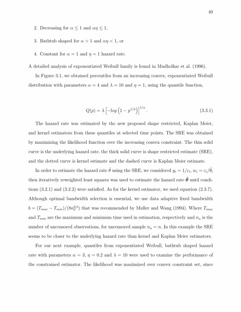
In Figure 3.1, we obtained percentiles from an increasing convex, exponentiated Weibull
distribution with parameters α = 4 and λ = 10 and η = 1, using the quantile function,
Q(p) = λ[
−log(
1 − p1/η)]1/α
. (3.3.1)
The hazard rate was estimated by the new proposed shape restricted, Kaplan Meier,
and kernel estimators from these quantiles at selected time points. The SRE was obtained
by maximizing the likelihood function over the increasing convex constraint. The thin solid
curve is the underlying hazard rate, the thick solid curve is shape restricted estimate (SRE),
and the dotted curve is kernel estimate and the dashed curve is Kaplan Meier estimate.
In order to estimate the hazard rate θ using the SRE, we considered yi = 1/ci, wi = ci/θi
then iteratively reweighted least squares was used to estimate the hazard rate θ until condi-
tions (3.2.1) and (3.2.2) were satisfied. As for the kernel estimator, we used equation (2.3.7).
Although optimal bandwidth selection is essential, we use data adaptive fixed bandwidth
b = (Tmax − Tmin)/(8n0.2U ) that was recommended by Muller and Wang (1994). Where Tmax
and Tmin are the maximum and minimum time used in estimation, respectively and nu is the
number of uncensored observations, for uncensored sample nu = n. In this example the SRE
seems to be closer to the underlying hazard rate than kernel and Kaplan Meier estimators.
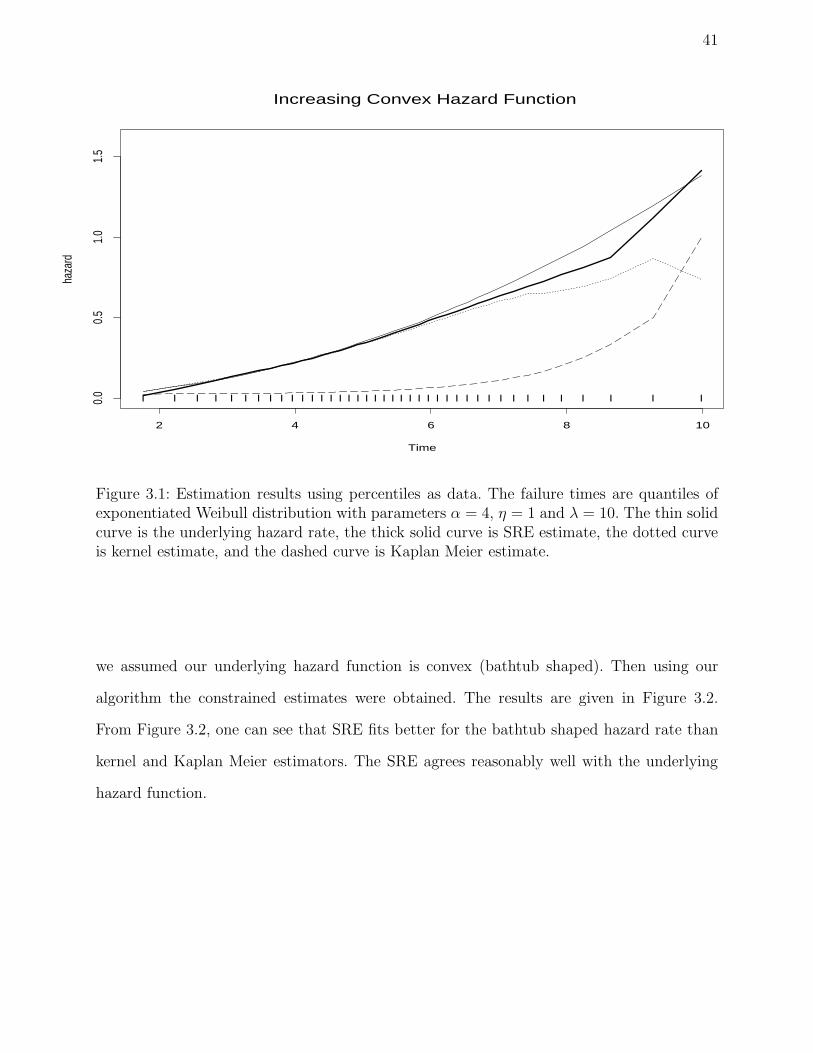
For our next example, quantiles from exponentiated Weibull, bathtub shaped hazard
rate with parameters α = 3, η = 0.2 and λ = 10 were used to examine the performance of
the constrained estimator. The likelihood was maximized over convex constraint set, since
41
Time
haza
rd
2 4 6 8 10
0.0
0.5
1.0
1.5
Increasing Convex Hazard Function
l l l l l l l l l l l l l l l l l l l l l l l l l l l l l l l l l l l l l l l l
Figure 3.1: Estimation results using percentiles as data. The failure times are quantiles ofexponentiated Weibull distribution with parameters α = 4, η = 1 and λ = 10. The thin solidcurve is the underlying hazard rate, the thick solid curve is SRE estimate, the dotted curveis kernel estimate, and the dashed curve is Kaplan Meier estimate.
we assumed our underlying hazard function is convex (bathtub shaped). Then using our
algorithm the constrained estimates were obtained. The results are given in Figure 3.2.
From Figure 3.2, one can see that SRE fits better for the bathtub shaped hazard rate than
kernel and Kaplan Meier estimators. The SRE agrees reasonably well with the underlying
hazard function.
42
Time
haza
rd
0 2 4 6 8
0.0
0.2
0.4
0.6
0.8
1.0
1.2
1.4
Convex Hazard Function
llll l l l l l l l l l l l l l l l l l l l l l l l l l l l l l l l l l l l l
Figure 3.2: Estimation results using percentiles as data. The failure times are quantiles ofexponentiated Weibull distribution with parameters α = 3, η = 0.2 and λ = 10. The thinsolid curve is the underlying hazard rate estimate, the thick solid curve is SRE estimate, thedotted curve is kernel estimate, and the dashed curve is Kaplan Meier estimate.
3.3.2 Quadratic hazard function
For our third example, we considered distribution with a polynomial hazard function. The
hazard function can be written as polynomial,
h(t) = β0 + β1t + · · · + βm−1tm−1
43
The survival function for the distribution is S(t) = exp[−H(t)] and the p.d.f is f(t) =
h(t)S(t) and the parameters β1, · · · , βm−1 must satisfy certain constraints since H(0) = 0
and H(∞) = ∞.
Distributions with m = 2 were discussed by Bain (1974). Recently, polynomial hazard
functions with m = 2, 3 and 4 were also discussed by Hess et al. (1999). For comparison
purpose and convenience, we chose quadratic concave up hazard functions. We followed
the methods used by Hess et al. (1999) to obtain the coefficients of the polynomial hazard
function. They simulated life times over [0,100], and specified h(t) = λ0h0(t), where λ0
was set so that S(t = 90) = 0.1 for n = 100. These values correspond to leaving about
10 patients at risk when t = 90. For quadratic concave up β0, β1 and β3 were selected to
achieve h0(0) = 1, h0(50) = 0 and h0(100) = 1. Then the inverse function ti = S−1(pi)
was used to obtain the percentile of failure times. Based on the computed failure times,
estimates of the underlying hazard function were obtained using the SRE, kernel, Kaplan
Meier estimators. The results of the estimates are shown on Figure 3.3. From the results
we see that our estimator agreed better with the underlying quadratic hazard function than
kernel and Kaplan Meier estimator except at the end points.
3.4 Right Censored Sample
The Direct Approach
Recall the random right censored data in chapter 2, section 2.2, on each of n individuals
we observe the pair(Xi, δi) where Xi = min(Ti, Zi) and δi = I(Ti ≤ Zi). The problem
considered here is estimation of f, F, or h by maximizing data from experiments involving
right censoring. Recall that the likelihood for right censored data is given by,
L =∏
f(xi)δiS(xi)
1−δi ,
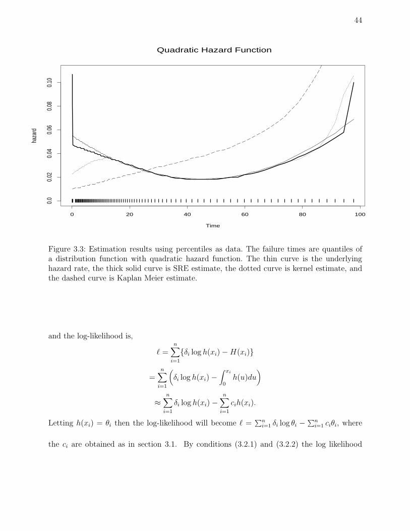
44
Time
haza
rd
0 20 40 60 80 100
0.0
0.02
0.04
0.06
0.08
0.10
Quadratic Hazard Function
llll lllllllllllllllllllllllllllllllllllllllllllllll l l l l l l l l l l l l l l l l l l l l l l l l l l l l l l l l l l l l l l l l l l l l
Figure 3.3: Estimation results using percentiles as data. The failure times are quantiles ofa distribution function with quadratic hazard function. The thin curve is the underlyinghazard rate, the thick solid curve is SRE estimate, the dotted curve is kernel estimate, andthe dashed curve is Kaplan Meier estimate.
and the log-likelihood is,
ℓ =n∑
i=1
δi log h(xi) − H(xi)
=n∑
i=1
(
δi log h(xi) −∫ xi
0h(u)du
)
≈n∑
i=1
δi log h(xi) −n∑
i=1
cih(xi).
Letting h(xi) = θi then the log-likelihood will become ℓ =∑n
i=1 δi log θi −∑n
i=1 ciθi, where
the ci are obtained as in section 3.1. By conditions (3.2.1) and (3.2.2) the log likelihood
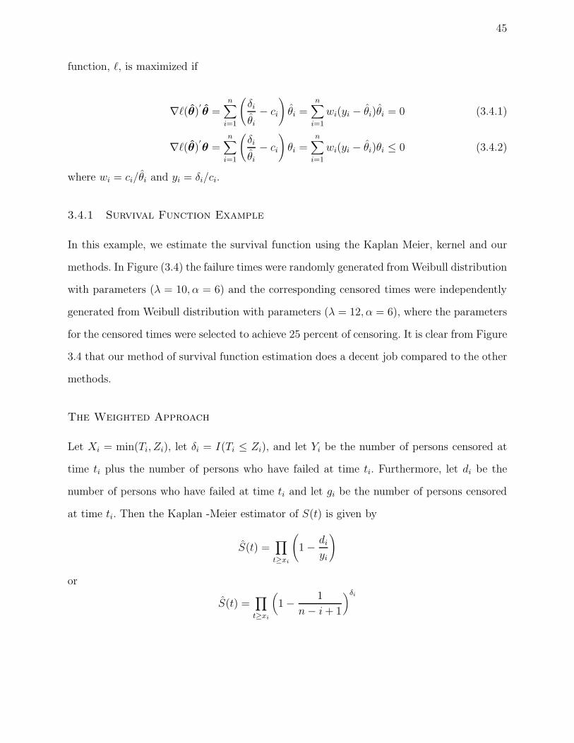
45
function, ℓ, is maximized if
∇ℓ(θ)′
θ =n∑
i=1
(
δi
θi
− ci
)
θi =n∑
i=1
wi(yi − θi)θi = 0 (3.4.1)
∇ℓ(θ)′
θ =n∑
i=1
(
δi
θi
− ci
)
θi =n∑
i=1
wi(yi − θi)θi ≤ 0 (3.4.2)
where wi = ci/θi and yi = δi/ci.
3.4.1 Survival Function Example
In this example, we estimate the survival function using the Kaplan Meier, kernel and our
methods. In Figure (3.4) the failure times were randomly generated from Weibull distribution
with parameters (λ = 10, α = 6) and the corresponding censored times were independently
generated from Weibull distribution with parameters (λ = 12, α = 6), where the parameters
for the censored times were selected to achieve 25 percent of censoring. It is clear from Figure
3.4 that our method of survival function estimation does a decent job compared to the other
methods.
The Weighted Approach
Let Xi = min(Ti, Zi), let δi = I(Ti ≤ Zi), and let Yi be the number of persons censored at
time ti plus the number of persons who have failed at time ti. Furthermore, let di be the
number of persons who have failed at time ti and let gi be the number of persons censored
at time ti. Then the Kaplan -Meier estimator of S(t) is given by
S(t) =∏
t≥xi
(
1 −di
yi
)
or
S(t) =∏
t≥xi
(
1 −1
n − i + 1
)δi
46
Time
Surv
ival
6 7 8 9 10 11 12
0.2
0.4
0.6
0.8
Survival Function Estimated by Different Methods
l l l ll l l l ll l l l l l l lll l l l l l l l lll l l ll l l l l l l
Figure 3.4: Comparison of Survival functions estimated by different methods. The thin solidcurve is the underlying survival function, the thick solid curve is the shape restricted estimate,the dotted curve is Kaplan Meier estimate and the dashed curve is kernel estimate.
with x1 < x2 < . . . < xn the order statistics of x′is and δi the associated index of xi. Here di
is 1 or 0 and gi is 0 or 1.
Satten and Datta (2000) have shown that the Kaplan Meier estimator can also be
expressed as an inverse probability of censoring weighted estimator. This approach was intro-
duced in Koul et al. (1981) and Robins and Rotnitzky (1992).
Let survival function for censoring is K(t) = P (Zi > t), using Kaplan -Meier approach K(t)
is given by,
K(t) =∏
t≥xi
(
1 −gi
yi
)
,
47
but we considered that the true failure times as censored times and their corresponding
censoring times as true failure times.
Then the inverse probability of censoring weighted estimator representation of the
Kaplan-Meier estimator is given by,
S(t) =1
n
n∑
i=1
δiI (xi > t)
K(xi−). (3.4.3)
If there were no censoring, the survival function could be estimated by the empirical
survival function,
S(t) =1
n
n∑
i=1
I (xi > t) .
The estimator given by (3.4.3) is an average of iid terms I(xi > t), each multiplied by
δ = I(ti ≤ zi) and weighted inversely by P (Zi ≥ ti). It is analogous to S(t), see Satten and
Datta (2000) for more discussion.
Recall that the log likelihood function of the hazard function is
ℓ =n∑
i=1
δi log h(xi) −n∑
i=1
cih(xi).
Now using the same approach as the survival function the likelihood for the censored data
can be approximated byn∑
i=1
δi log h(xi)
K(xi−)−
n∑
i=1
cih(xi)
K(xi−)
=n∑
i=1
di log(h(xi)) −n∑
i=1
eih(xi)
where di = δi/K(xi−) and ei = ci/K(xi−)
Conditions (3.2.1) and (3.2.2) will be
n∑
i=1
1
K(xi−)
(
δ1
θi
− ci
)
θi =n∑
i=1
wi(yi − θi)θi = 0 (3.4.4)
48
n∑
i=1
1
K(xi−)
(
δi
θi
− ci
)
θi =n∑
i=1
wi(yi − θi)θi ≤ 0 (3.4.5)
where wi = ci/K(xi−)θi and yi = δi/ci.
Comparing the direct and weighted approaches, we can clearly see that they are equivalent
except for the weights. The latter form is suitable for extending the methodology to the case
of dependent censoring. Dependent censoring occur, for example, if there are covariates that
affect both the hazard of failure and hazard of being censored. Satten, et al. (2001) is a good
reference for the dependent censoring case. We plan to extend our results to incorporate
dependent censoring in the future. This can be easily handled by the weighted approach.
Chapter 4
SIMULATION STUDIES AND APPLICATION TO REAL DATA SETS
4.1 Simulation Results
In this chapter we evaluate the performance of the shape restricted estimator (SRE) using
simulation studies. This allows us to compare the results of the estimates obtained by kernel,
Kaplan Meier estimator and our estimator to the values of the underlying hazard function.
The simulation was done for two different shapes of hazard function namely: nondecreasing
convex and convex (bathtub shaped).
The failure times were generated from a Weibull distribution with shape and scale param-
eters 3 and 6, respectively, for the increasing convex hazard function. To implement random
censorship, we independently generated corresponding censoring times from Weibull distri-
bution with scale and shape parameters α and λ, respectively, where α and λ were selected
to achieve a given proportion of censoring: 0 percent, 25 percent and 50 percent. The kernel,
Kaplan Meier and SRE were then computed based on the generated observed lifetimes for
sample sizes 25, 50 and 75 at different levels of censoring.
Similarly, for the convex (bathtub shaped) hazard function, the failure times were gener-
ated from an exponentiated Weibull distribution with parameters α = 3, λ = 6 and η = 0.20
and the corresponding censoring times were generated independently from exponentiated
Weibull distribution with α, λ and η, where α, λ and η were chosen to yield about, 0, 25
and 50 censoring. The simulation repeated N=1000 times for each setting.
49
50
To summarize our simulation results, we computed the overall mean squared error
(OMSE), the average were taken over 1000 simulation and n observed time points. The
OMSE was computed without the largest and smallest observed time, because at the end
points our estimator has spikes. Results from the simulations are presented in Tables 4.1
and 4.2. All the results are rounded to nearest thousandth. Tables 4.1 and 4.2 show the
OMSE of SRE, kernel and Kaplan Meier for different levels of censoring and sample sizes
25, 50 and 75.
We also computed point-wise mean squared errors (MSE) and bias for our estimator
(SRE), kernel and Kaplan Meier at selected grid points between 1.5 and 6.5 with 0.5 incre-
ment, and between 1.00 and 6.5 with 0.5 increment for increasing convex and convex, respec-
tively. The results are given in Tables 4.4-4.7.
The bias and mean squared error (MSE) and standard deviation (SD) at the grid points
are computed as:
Bias(t) =
∑Ni=1 h(t)
N− h(t),
MSE(t) =
∑Ni=1
(
h(t) − h(t))2
N.
SD(t) =
√
√
√
√
∑Ni=1
(
h(t) − h(t))2
N − 1,
respectively.
The results from Tables 4.1 and 4.2, demonstrated that the SRE performed fairly well in
all cases. It is better than kernel and Kaplan Meier when the hazard function is estimated
without spikes. For a high rate of censoring, the performance of the SRE compared to the
kernel method is nearly the same. The Kaplan Meier estimator performed poorly in all cases.
From Tables 4.4-4.7 we found that the SRE has smaller MSE than Kaplan Meier. When
the level of censoring is low and if the MSE computed at the grid point which are not close
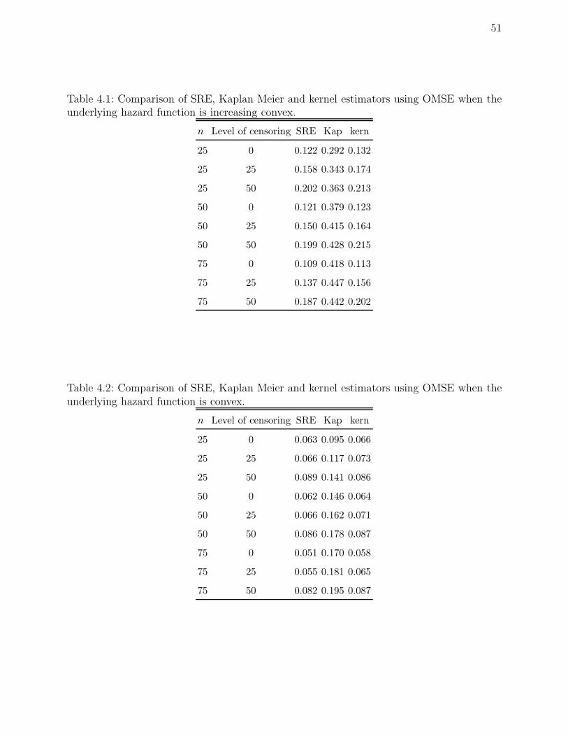
51
Table 4.1: Comparison of SRE, Kaplan Meier and kernel estimators using OMSE when theunderlying hazard function is increasing convex.
n Level of censoring SRE Kap kern
25 0 0.122 0.292 0.132
25 25 0.158 0.343 0.174
25 50 0.202 0.363 0.213
50 0 0.121 0.379 0.123
50 25 0.150 0.415 0.164
50 50 0.199 0.428 0.215
75 0 0.109 0.418 0.113
75 25 0.137 0.447 0.156
75 50 0.187 0.442 0.202
Table 4.2: Comparison of SRE, Kaplan Meier and kernel estimators using OMSE when theunderlying hazard function is convex.
n Level of censoring SRE Kap kern
25 0 0.063 0.095 0.066
25 25 0.066 0.117 0.073
25 50 0.089 0.141 0.086
50 0 0.062 0.146 0.064
50 25 0.066 0.162 0.071
50 50 0.086 0.178 0.087
75 0 0.051 0.170 0.058
75 25 0.055 0.181 0.065
75 50 0.082 0.195 0.087

52
to end points the SRE performed better than kernel for both increasing convex and convex
hazard functions. As for a higher censoring rate, the kernel has smaller bias and MSE than
the SRE, in particular if the MSE and bias are calculated at the end points. This is not
surprising because SRE spikes at the endpoints. It can also be easily noted that MSE and
bias become relatively larger whenever that rate of censoring increase. If we investigate the
performance of the estimators in terms of bias, the judgment as to which estimator is better
may not be so clear cut, at 0 and 25 percent of censoring. At at the end points and for
higher level of censoring kernel perform better than SRE. We also see that the MSE and
bias decrease as n increases as expected.
To compare the performance of weighted and direct approaches (see Chapter 3, pp. 43-
46), we computed overall MSE and average bias for two samples and two levels of censoring.
The results are given in Table 4.3. The average were taken over 1000 simulations and the
selected time points. From the results of the simulation, the weighted approach performed
slightly better than the direct approach in all cases.
4.2 Application To Real Data Sets
In this section we illustrate how the proposed methodology works by using different data
sets.
Head and Neck Example
For our first real data example we used a data set from a clinical trial conducted by Northern
Oncology Group, discussed by Efron (1988). The data represent the survival times of 51
head and neck cancer patients under treatment A, who were given radiation therapy. Nine
patients were lost to follow up and were considered as censored. The data from Efron (1988)
are reproduced in Table A.1 in the appendices. Efron observed that the empirical hazard
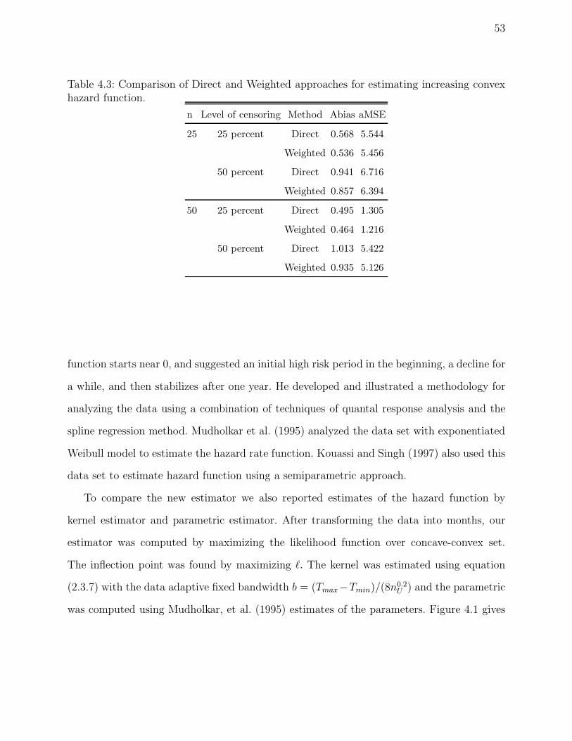
53
Table 4.3: Comparison of Direct and Weighted approaches for estimating increasing convexhazard function.
n Level of censoring Method Abias aMSE
25 25 percent Direct 0.568 5.544
Weighted 0.536 5.456
50 percent Direct 0.941 6.716
Weighted 0.857 6.394
50 25 percent Direct 0.495 1.305
Weighted 0.464 1.216
50 percent Direct 1.013 5.422
Weighted 0.935 5.126
function starts near 0, and suggested an initial high risk period in the beginning, a decline for
a while, and then stabilizes after one year. He developed and illustrated a methodology for
analyzing the data using a combination of techniques of quantal response analysis and the
spline regression method. Mudholkar et al. (1995) analyzed the data set with exponentiated
Weibull model to estimate the hazard rate function. Kouassi and Singh (1997) also used this
data set to estimate hazard function using a semiparametric approach.
To compare the new estimator we also reported estimates of the hazard function by
kernel estimator and parametric estimator. After transforming the data into months, our
estimator was computed by maximizing the likelihood function over concave-convex set.
The inflection point was found by maximizing ℓ. The kernel was estimated using equation
(2.3.7) with the data adaptive fixed bandwidth b = (Tmax−Tmin)/(8n0.2U ) and the parametric
was computed using Mudholkar, et al. (1995) estimates of the parameters. Figure 4.1 gives
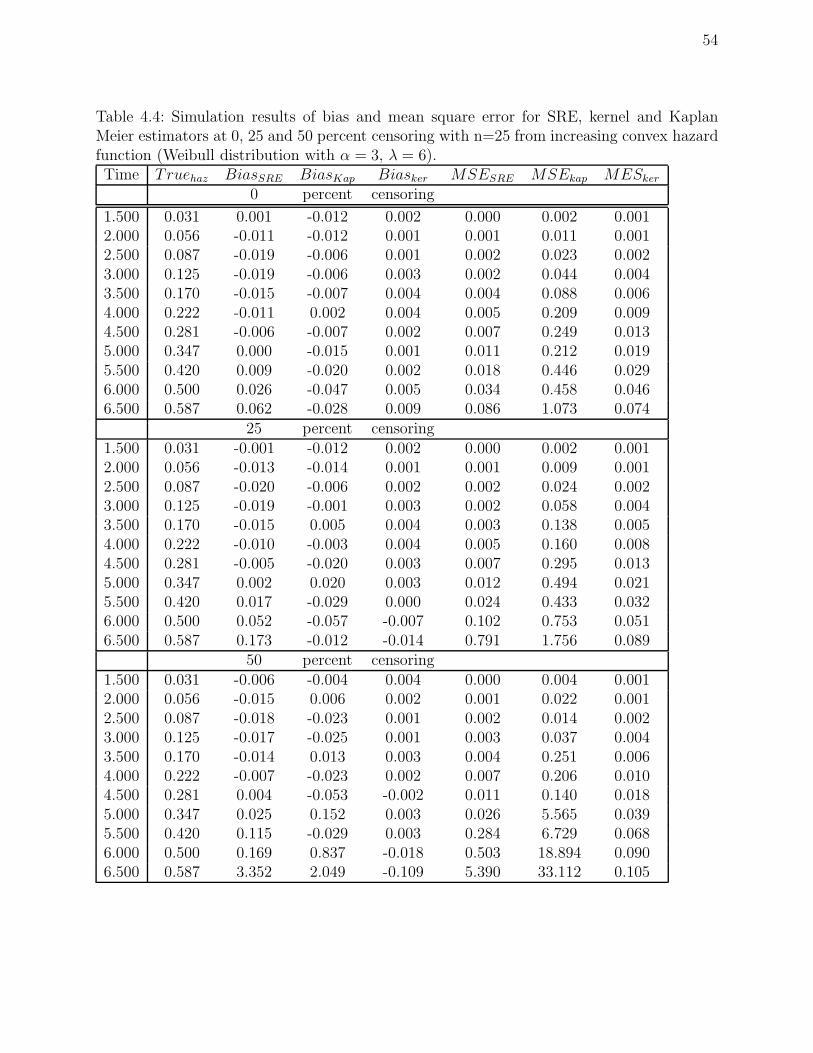
54
Table 4.4: Simulation results of bias and mean square error for SRE, kernel and KaplanMeier estimators at 0, 25 and 50 percent censoring with n=25 from increasing convex hazardfunction (Weibull distribution with α = 3, λ = 6).Time Truehaz BiasSRE BiasKap Biasker MSESRE MSEkap MESker
0 percent censoring
1.500 0.031 0.001 -0.012 0.002 0.000 0.002 0.0012.000 0.056 -0.011 -0.012 0.001 0.001 0.011 0.0012.500 0.087 -0.019 -0.006 0.001 0.002 0.023 0.0023.000 0.125 -0.019 -0.006 0.003 0.002 0.044 0.0043.500 0.170 -0.015 -0.007 0.004 0.004 0.088 0.0064.000 0.222 -0.011 0.002 0.004 0.005 0.209 0.0094.500 0.281 -0.006 -0.007 0.002 0.007 0.249 0.0135.000 0.347 0.000 -0.015 0.001 0.011 0.212 0.0195.500 0.420 0.009 -0.020 0.002 0.018 0.446 0.0296.000 0.500 0.026 -0.047 0.005 0.034 0.458 0.0466.500 0.587 0.062 -0.028 0.009 0.086 1.073 0.074
25 percent censoring1.500 0.031 -0.001 -0.012 0.002 0.000 0.002 0.0012.000 0.056 -0.013 -0.014 0.001 0.001 0.009 0.0012.500 0.087 -0.020 -0.006 0.002 0.002 0.024 0.0023.000 0.125 -0.019 -0.001 0.003 0.002 0.058 0.0043.500 0.170 -0.015 0.005 0.004 0.003 0.138 0.0054.000 0.222 -0.010 -0.003 0.004 0.005 0.160 0.0084.500 0.281 -0.005 -0.020 0.003 0.007 0.295 0.0135.000 0.347 0.002 0.020 0.003 0.012 0.494 0.0215.500 0.420 0.017 -0.029 0.000 0.024 0.433 0.0326.000 0.500 0.052 -0.057 -0.007 0.102 0.753 0.0516.500 0.587 0.173 -0.012 -0.014 0.791 1.756 0.089
50 percent censoring1.500 0.031 -0.006 -0.004 0.004 0.000 0.004 0.0012.000 0.056 -0.015 0.006 0.002 0.001 0.022 0.0012.500 0.087 -0.018 -0.023 0.001 0.002 0.014 0.0023.000 0.125 -0.017 -0.025 0.001 0.003 0.037 0.0043.500 0.170 -0.014 0.013 0.003 0.004 0.251 0.0064.000 0.222 -0.007 -0.023 0.002 0.007 0.206 0.0104.500 0.281 0.004 -0.053 -0.002 0.011 0.140 0.0185.000 0.347 0.025 0.152 0.003 0.026 5.565 0.0395.500 0.420 0.115 -0.029 0.003 0.284 6.729 0.0686.000 0.500 0.169 0.837 -0.018 0.503 18.894 0.0906.500 0.587 3.352 2.049 -0.109 5.390 33.112 0.105
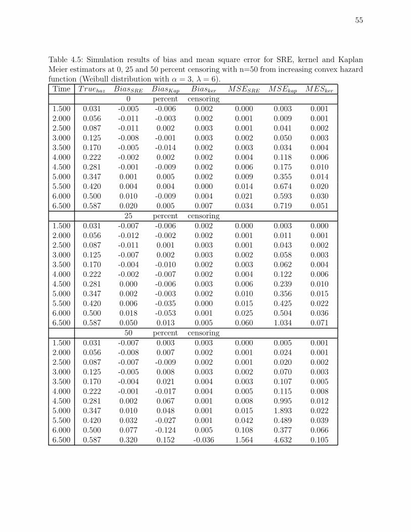
55
Table 4.5: Simulation results of bias and mean square error for SRE, kernel and KaplanMeier estimators at 0, 25 and 50 percent censoring with n=50 from increasing convex hazardfunction (Weibull distribution with α = 3, λ = 6).Time Truehaz BiasSRE BiasKap Biasker MSESRE MSEkap MESker
0 percent censoring1.500 0.031 -0.005 -0.006 0.002 0.000 0.003 0.0012.000 0.056 -0.011 -0.003 0.002 0.001 0.009 0.0012.500 0.087 -0.011 0.002 0.003 0.001 0.041 0.0023.000 0.125 -0.008 -0.001 0.003 0.002 0.050 0.0033.500 0.170 -0.005 -0.014 0.002 0.003 0.034 0.0044.000 0.222 -0.002 0.002 0.002 0.004 0.118 0.0064.500 0.281 -0.001 -0.009 0.002 0.006 0.175 0.0105.000 0.347 0.001 0.005 0.002 0.009 0.355 0.0145.500 0.420 0.004 0.004 0.000 0.014 0.674 0.0206.000 0.500 0.010 -0.009 0.004 0.021 0.593 0.0306.500 0.587 0.020 0.005 0.007 0.034 0.719 0.051
25 percent censoring1.500 0.031 -0.007 -0.006 0.002 0.000 0.003 0.0002.000 0.056 -0.012 -0.002 0.002 0.001 0.011 0.0012.500 0.087 -0.011 0.001 0.003 0.001 0.043 0.0023.000 0.125 -0.007 0.002 0.003 0.002 0.058 0.0033.500 0.170 -0.004 -0.010 0.002 0.003 0.062 0.0044.000 0.222 -0.002 -0.007 0.002 0.004 0.122 0.0064.500 0.281 0.000 -0.006 0.003 0.006 0.239 0.0105.000 0.347 0.002 -0.003 0.002 0.010 0.356 0.0155.500 0.420 0.006 -0.035 0.000 0.015 0.425 0.0226.000 0.500 0.018 -0.053 0.001 0.025 0.504 0.0366.500 0.587 0.050 0.013 0.005 0.060 1.034 0.071
50 percent censoring1.500 0.031 -0.007 0.003 0.003 0.000 0.005 0.0012.000 0.056 -0.008 0.007 0.002 0.001 0.024 0.0012.500 0.087 -0.007 -0.009 0.002 0.001 0.020 0.0023.000 0.125 -0.005 0.008 0.003 0.002 0.070 0.0033.500 0.170 -0.004 0.021 0.004 0.003 0.107 0.0054.000 0.222 -0.001 -0.017 0.004 0.005 0.115 0.0084.500 0.281 0.002 0.067 0.001 0.008 0.995 0.0125.000 0.347 0.010 0.048 0.001 0.015 1.893 0.0225.500 0.420 0.032 -0.027 0.001 0.042 0.489 0.0396.000 0.500 0.077 -0.124 0.005 0.108 0.377 0.0666.500 0.587 0.320 0.152 -0.036 1.564 4.632 0.105
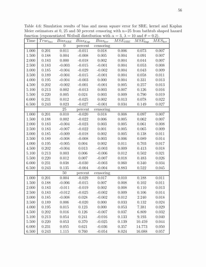
56
Table 4.6: Simulation results of bias and mean square error for SRE, kernel and KaplanMeier estimators at 0, 25 and 50 percent censoring with n=25 from bathtub shaped hazardfunction (exponentiated Weibull distribution with α = 3, λ = 10 and θ = 0.2).Time Truehaz BiasSRE BiasKap Biasker MSESRE MSEkap MESker
0 percent censoring1.000 0.201 0.011 -0.011 0.018 0.006 0.073 0.0071.500 0.188 0.004 -0.008 0.005 0.004 0.091 0.0072.000 0.183 0.000 -0.018 0.002 0.004 0.044 0.0072.500 0.183 -0.003 -0.015 -0.001 0.004 0.053 0.0083.000 0.185 -0.004 -0.029 -0.002 0.004 0.043 0.0093.500 0.189 -0.004 -0.015 -0.001 0.004 0.058 0.0114.000 0.195 -0.004 -0.003 0.000 0.004 0.331 0.0134.500 0.202 -0.002 -0.001 -0.001 0.005 0.257 0.0135.100 0.213 0.002 -0.013 0.003 0.007 0.126 0.0165.500 0.220 0.005 0.024 0.003 0.009 0.790 0.0196.000 0.231 0.012 -0.025 0.002 0.013 0.078 0.0226.500 0.243 0.023 -0.027 -0.001 0.034 0.149 0.027
25 percent censoring1.000 0.201 0.010 -0.020 0.018 0.008 0.097 0.0071.500 0.188 0.002 -0.022 0.006 0.005 0.062 0.0072.000 0.183 -0.004 -0.023 0.003 0.005 0.061 0.0082.500 0.183 -0.007 -0.022 0.001 0.005 0.065 0.0093.000 0.185 -0.009 -0.018 0.002 0.005 0.138 0.0113.500 0.189 -0.008 -0.008 0.003 0.006 0.089 0.0144.000 0.195 -0.005 0.004 0.002 0.011 0.703 0.0174.500 0.202 -0.004 0.013 -0.003 0.009 0.413 0.0185.100 0.213 0.003 0.006 -0.006 0.012 0.502 0.0215.500 0.220 0.012 0.007 -0.007 0.018 0.483 0.0266.000 0.231 0.038 -0.030 -0.003 0.060 0.340 0.0346.500 0.243 0.135 -0.004 -0.004 0.883 0.522 0.045
50 percent censoring1.000 0.201 0.004 -0.029 0.017 0.010 0.188 0.0111.500 0.188 -0.006 -0.015 0.007 0.008 0.102 0.0112.000 0.183 -0.011 -0.019 0.002 0.008 0.110 0.0132.500 0.183 -0.012 -0.025 -0.002 0.009 0.106 0.0143.000 0.185 -0.008 0.028 -0.002 0.012 2.240 0.0183.500 0.189 0.006 -0.020 0.000 0.033 0.132 0.0244.000 0.195 0.015 0.123 0.000 0.053 7.381 0.0294.500 0.202 0.016 0.126 -0.007 0.037 6.809 0.0325.100 0.213 0.054 0.241 -0.016 0.133 9.193 0.0405.500 0.220 0.053 0.370 -0.025 0.139 10.459 0.0446.000 0.231 0.055 0.621 -0.036 0.357 14.773 0.0506.500 0.243 1.115 0.760 -0.054 8.024 16.088 0.057
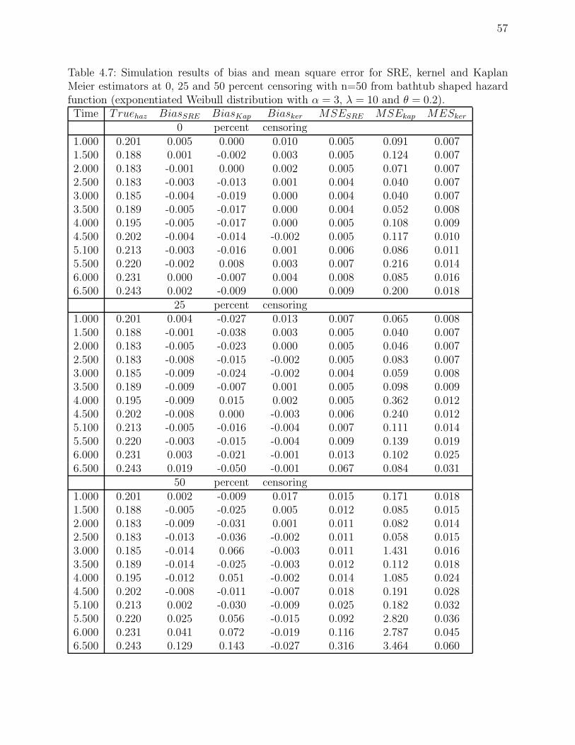
57
Table 4.7: Simulation results of bias and mean square error for SRE, kernel and KaplanMeier estimators at 0, 25 and 50 percent censoring with n=50 from bathtub shaped hazardfunction (exponentiated Weibull distribution with α = 3, λ = 10 and θ = 0.2).Time Truehaz BiasSRE BiasKap Biasker MSESRE MSEkap MESker
0 percent censoring1.000 0.201 0.005 0.000 0.010 0.005 0.091 0.0071.500 0.188 0.001 -0.002 0.003 0.005 0.124 0.0072.000 0.183 -0.001 0.000 0.002 0.005 0.071 0.0072.500 0.183 -0.003 -0.013 0.001 0.004 0.040 0.0073.000 0.185 -0.004 -0.019 0.000 0.004 0.040 0.0073.500 0.189 -0.005 -0.017 0.000 0.004 0.052 0.0084.000 0.195 -0.005 -0.017 0.000 0.005 0.108 0.0094.500 0.202 -0.004 -0.014 -0.002 0.005 0.117 0.0105.100 0.213 -0.003 -0.016 0.001 0.006 0.086 0.0115.500 0.220 -0.002 0.008 0.003 0.007 0.216 0.0146.000 0.231 0.000 -0.007 0.004 0.008 0.085 0.0166.500 0.243 0.002 -0.009 0.000 0.009 0.200 0.018
25 percent censoring1.000 0.201 0.004 -0.027 0.013 0.007 0.065 0.0081.500 0.188 -0.001 -0.038 0.003 0.005 0.040 0.0072.000 0.183 -0.005 -0.023 0.000 0.005 0.046 0.0072.500 0.183 -0.008 -0.015 -0.002 0.005 0.083 0.0073.000 0.185 -0.009 -0.024 -0.002 0.004 0.059 0.0083.500 0.189 -0.009 -0.007 0.001 0.005 0.098 0.0094.000 0.195 -0.009 0.015 0.002 0.005 0.362 0.0124.500 0.202 -0.008 0.000 -0.003 0.006 0.240 0.0125.100 0.213 -0.005 -0.016 -0.004 0.007 0.111 0.0145.500 0.220 -0.003 -0.015 -0.004 0.009 0.139 0.0196.000 0.231 0.003 -0.021 -0.001 0.013 0.102 0.0256.500 0.243 0.019 -0.050 -0.001 0.067 0.084 0.031
50 percent censoring1.000 0.201 0.002 -0.009 0.017 0.015 0.171 0.0181.500 0.188 -0.005 -0.025 0.005 0.012 0.085 0.0152.000 0.183 -0.009 -0.031 0.001 0.011 0.082 0.0142.500 0.183 -0.013 -0.036 -0.002 0.011 0.058 0.0153.000 0.185 -0.014 0.066 -0.003 0.011 1.431 0.0163.500 0.189 -0.014 -0.025 -0.003 0.012 0.112 0.0184.000 0.195 -0.012 0.051 -0.002 0.014 1.085 0.0244.500 0.202 -0.008 -0.011 -0.007 0.018 0.191 0.0285.100 0.213 0.002 -0.030 -0.009 0.025 0.182 0.0325.500 0.220 0.025 0.056 -0.015 0.092 2.820 0.0366.000 0.231 0.041 0.072 -0.019 0.116 2.787 0.0456.500 0.243 0.129 0.143 -0.027 0.316 3.464 0.060
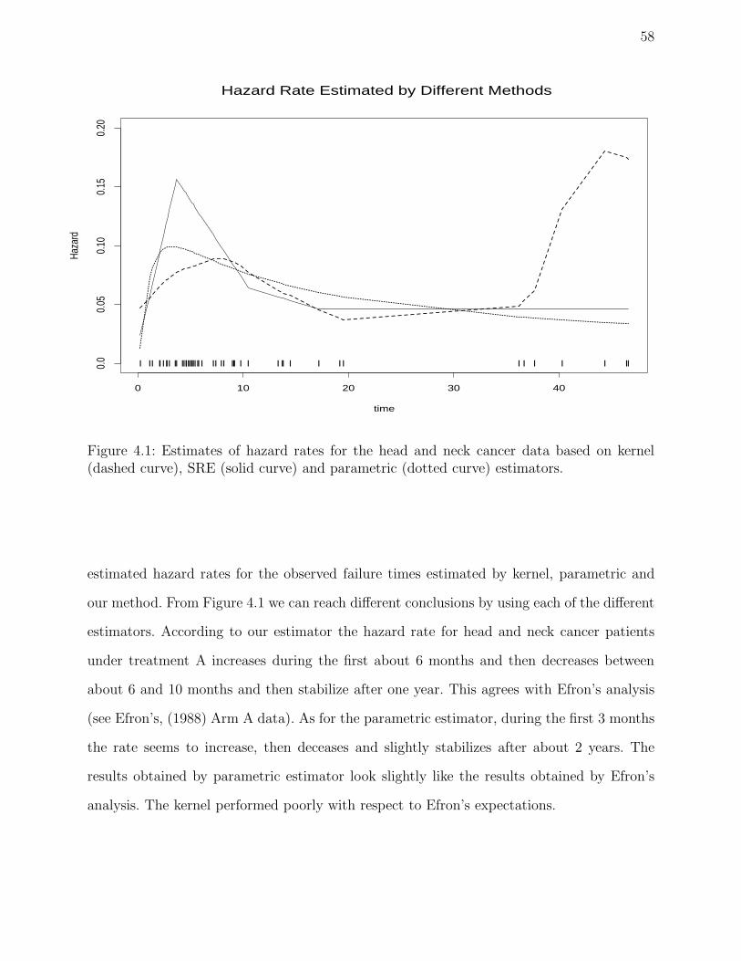
58
time
Haza
rd
0 10 20 30 40
0.0
0.05
0.10
0.15
0.20
Hazard Rate Estimated by Different Methods
l ll ll l lll ll llllllllllll l ll ll lll l l l ll l l l l l l l l l ll
Figure 4.1: Estimates of hazard rates for the head and neck cancer data based on kernel(dashed curve), SRE (solid curve) and parametric (dotted curve) estimators.
estimated hazard rates for the observed failure times estimated by kernel, parametric and
our method. From Figure 4.1 we can reach different conclusions by using each of the different
estimators. According to our estimator the hazard rate for head and neck cancer patients
under treatment A increases during the first about 6 months and then decreases between
about 6 and 10 months and then stabilize after one year. This agrees with Efron’s analysis
(see Efron’s, (1988) Arm A data). As for the parametric estimator, during the first 3 months
the rate seems to increase, then deceases and slightly stabilizes after about 2 years. The
results obtained by parametric estimator look slightly like the results obtained by Efron’s
analysis. The kernel performed poorly with respect to Efron’s expectations.
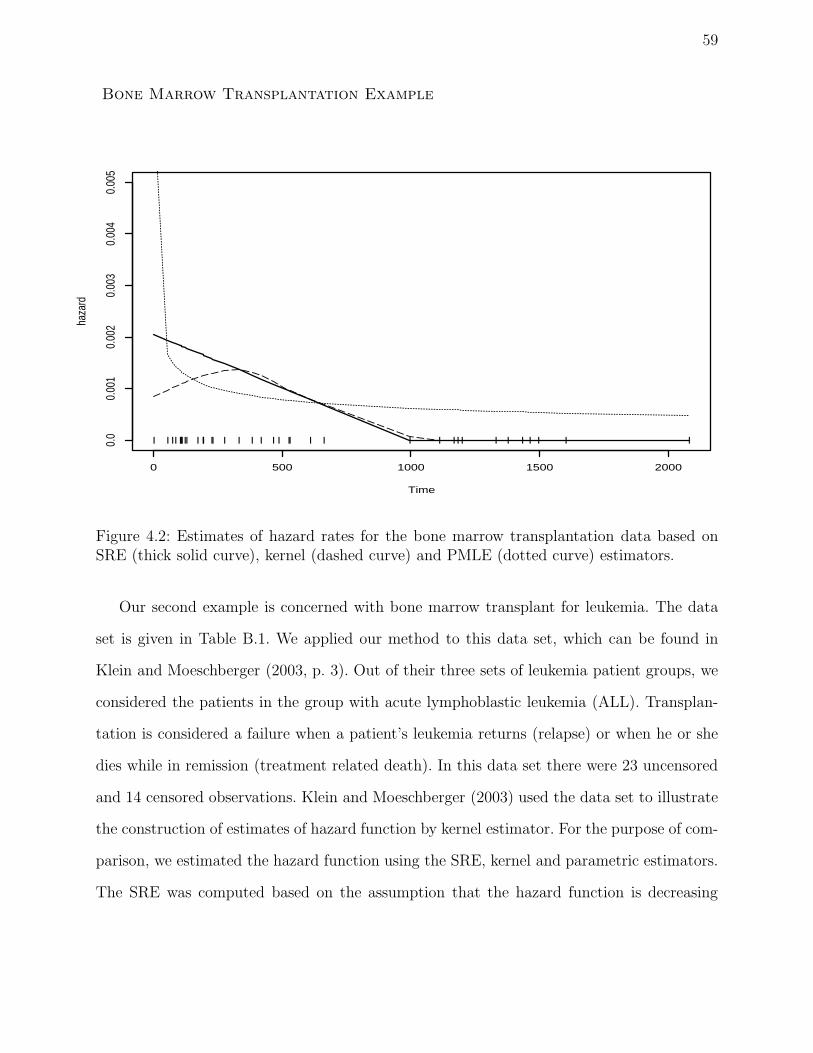
59
Bone Marrow Transplantation Example
Time
haza
rd
0 500 1000 1500 2000
0.0
0.00
10.
002
0.00
30.
004
0.00
5
l l ll llllll l ll ll l l l l l l ll l l l l l l l l l l l l l l
Figure 4.2: Estimates of hazard rates for the bone marrow transplantation data based onSRE (thick solid curve), kernel (dashed curve) and PMLE (dotted curve) estimators.
Our second example is concerned with bone marrow transplant for leukemia. The data
set is given in Table B.1. We applied our method to this data set, which can be found in
Klein and Moeschberger (2003, p. 3). Out of their three sets of leukemia patient groups, we
considered the patients in the group with acute lymphoblastic leukemia (ALL). Transplan-
tation is considered a failure when a patient’s leukemia returns (relapse) or when he or she
dies while in remission (treatment related death). In this data set there were 23 uncensored
and 14 censored observations. Klein and Moeschberger (2003) used the data set to illustrate
the construction of estimates of hazard function by kernel estimator. For the purpose of com-
parison, we estimated the hazard function using the SRE, kernel and parametric estimators.
The SRE was computed based on the assumption that the hazard function is decreasing
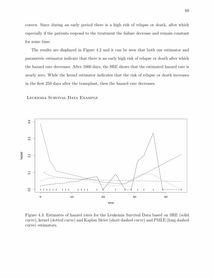
60
convex. Since during an early period there is a high risk of relapse or death, after which
especially if the patients respond to the treatment the failure decrease and remain constant
for some time.
The results are displayed in Figure 4.2 and it can be seen that both our estimator and
parametric estimator indicate that there is an early high risk of relapse or death after which
the hazard rate decreases. After 1000 days, the SRE shows that the estimated hazard rate is
nearly zero. While the kernel estimator indicates that the risk of relapse or death increases
in the first 250 days after the transplant, then the hazard rate decreases.
Leukemia Survival Data Example
time
haza
rd
0 10 20 30 40
0.0
0.1
0.2
0.3
0.4
l l l l l l l l l l l l l l l l l l l l l l l
Figure 4.3: Estimates of hazard rates for the Leukemia Survival Data based on SRE (solidcurve), kernel (dotted curve) and Kaplan Meier (short dashed curve) and PMLE (long dashedcurve) estimators.
61
This data set is taken from Lee (1980, Table 3.3, p. 72). Seventy-one adult patients
with acute leukemia (ALL) and acute myeloblastic Leukemia (AML) were studied at M.D.
Anderson Hospital and Tumor Institute (Hart et al. 1977). The data set is reproduced in
Table C.1. There were some covariates in the data set, in this study we consider the survival
of the patients from diagnosis of acute myeloblastic Leukemia (AML) and survival status
(life or death). There were 51 observations, of which 6 are censored. Based on the nature of
patients with Leukemia, it can be assumed that the bathtub shaped hazard function may
better describe the shape of the hazard function. Muller and Wang (1994) used this data set
to estimate the hazard function using kernel estimator with varying bandwidths. The result
of Muller and Wang (1994) seems to indicate a bathtub shaped hazard function. Based
on the assumption that the data have a bathtub shaped, estimates of the hazard function
were obtained using SRE. For comparison purpose we also reported estimates of the hazard
function by kernel, parametric, and Kaplan Meier estimators. The results are displayed in
Figure 4.3.
Chapter 5
TESTING FOR SHAPE RESTRICTED HAZARD FUNCTION USING
RESAMPLING TECHNIQUES
In this chapter, we study the problem of testing whether survival times can be modeled
by a certain parametric family such as Weibull, when shape restrictions such as monotonicity,
concavity or convexity are imposed on the hazard rate function. Weibull is commonly used in
statistical analysis of lifetimes (Cohen, 1965). It is generally adequate for modeling monotone
hazard rate functions. On the other hand, if we could reject the null hypothesis that the
hazard is from this parametric family, then the resulting parametric hazard estimate is
inaccurate. For instance, the Weibull family is inappropriate when the hazard rate is indicated
to be unimodal or bath-tub shape (Mudholkar et al., 1996).
In other words, we consider to test the hypothesis that the lifetimes come from a pop-
ulation with a parametric hazard rate function such as Weibull against a shape restricted
alternative that comprises a broad range of hazard functions. The alternative may be appro-
priate when the shape of parametric hazard is not constant and monotone.
A number of approaches have been used to test the equality of hazard or survival functions
for uncensored and censored data. There is a large literature on parametric methods which
lean heavily on likelihood methods for exponential distributions, for two or three parameter
Weibull models, and for other distributions such as log-logistic, log-normal and gamma.
These approaches are summarized in Lawless (1988), and Kalbfleisch and Prentice (1996).
The first nonparametric statistics that gained widespread usage in comparing two or more
hazard or survival functions for censored data were those proposed by Gehan (1965), who
62
63
made a generalization of Wilcoxon rank sum statistics, and Mantel (1966) also proposed
log-rank statistics which became the most commonly used two sample test statistics for
censored data. Many other authors have also considered nonparametric tests for equality of
two or more hazard or survival functions. For example, Chikkagoudar and Shuster, (1974)
proposed a rank test for comparison of failure rate. Bickel and Rosenblatt (1973) suggested
a Kolmogorov and Smirnov type test statistics based on maximal absolute deviation and
mean squared errors for censored data.
Most papers in the literature on shape restricted hazard rate function estimation, how-
ever, focus on testing the null hypothesis of a constant hazard rate versus the alternative of a
nondecreasing. For example, in the uncensored case, testing for a constant hazard rate versus
a nondecreasing has been considered by Bickel and Doksum (1969). Barlow and Porschan
(1969) extended these tests to handle Type I censored data. Hall et al. (2000) also proposed
a nonparametric test based on evaluating the distance between the monotonized estimator
and the standard kernel estimator. More recently, Xiong et al. (2004) presented the likeli-
hood ratio test for testing the null hypothesis that the hazard rate is constant against the
alternative that is increasing.
Hypothesis testing involving maximum likelihood estimates usually are tested by means
of the likelihood ratio statistic. Under some regularity conditions, the likelihood ratio statistic
is asymptotically chi-square distributed. For our case, we can not apply this scheme since
we are avoiding a complete specification of the likelihoods. Instead we plan to compare the
hazard function estimates obtained under shape restriction as was described in chapter 3
with its parametric counterpart using log rank and Kolmogorov’s goodness-of-fit.
We are using resampling based computation to conduct our tests since the asymptotic
distributions of the test statistics in these problems are largely intractable. The form of the
resampling scheme will depend on the null hypothesis to be tested. There are many ways
to use resampling scheme for hypothesis testing. In this dissertation, however, we use the
64
bootstrap p-values approach since it is a convenient way to perform bootstrap inferences
(Davidson and MacKinnon, 1996).
In this chapter, we investigate a number of testing problems. Then we discuss resampling
techniques and describe the bootstrapping method. The last section deals with a number
of simulation studies and an application to real data sets to check the performance of the
different test statistics under different alternatives.
5.1 Test Statistics
1. Consider testing the hypotheses,
H0 : h(t) = hpar(t)
against
HA : h(t) 6= hpar(t)
for all 0 ≤ t ≤ τ ; τ could be a fixed (nonrandom) time point although in practice, it
is often taken to be the largest observed study times. Here hpar is the hypothesized
parametric hazard function. The following log rank test statistic can be used.
Z(τ) =∫ τ
0W (s)h(s) − hpar(s)ds, (5.1.1)
where W (ti) is a weight function. The most popular choices are W (t) = Y (t) and
WFH(t) = S0(t)p[1 − S0(t)]
q. The latter one was proposed by Harrington and Fleming
(1982). The S0 is the null hypothesis survival function, p ≥ 0 and q ≥ 0, and Y (ti) is
the number of surviving individuals under study prior to the observed event time ti.
The above test statistic is found in Klein and Moeschberger (2003, chapter 7).
The weight function for the test statistics (5.1.1) was taken to be w(t) = S0(t) (1 − S0(t)).
Since our estimator may have spikes at the end points this assigns less weight to early
65
and late differences between h(t) and hpar(t). In other words, this puts more weights
on the differences of h(t) and h(t)par in the mid-range.
2. Consider Kolmogorov’s goodness-of-fit type testing problems where one tests a speci-
fied null hypothesis,
H0 : S(t) = S0(t)
against
HA : S(t) 6= S0(t).
In a general sense, this problem is the same as the previous one if indeed S0 has
unspecified parameters that need to be estimated except that the hypotheses are spec-
ified in terms of survival functions rather than the hazard rates. However, we may
consider a different test statistic that is in the form of a Kolmogorov’s goodness-of-fit
test. The test evaluates the closeness of the constrained survival function S(t) to the
hypothesized S0(t):
Dn = sup|S(t) − S0(t)|. (5.1.2)
3. For an important special case, one can indeed use a likelihood ratio approach. This is
the situation if the hazard function under H0 is increasing linear and the alternative is
increasing convex. In the case of regression data, Meyer (2003) showed that likelihood
ratio tests of linear versus convex regression functions known to have a mixture of beta
random variables. For further details see Meyer (2003).
66
5.2 Resampling Approach
The asymptotic distributions of the test statistics proposed in the previous section are not
only expected to be complicated but also intractable since they will involve parameters of
the censoring distribution and we have only approximated likelihood function. In such situ-
ations, resampling may be a practical and appealing alternative. The form of the resampling
scheme will depend on the null hypothesis to be tested. Although there are many ways to
use resampling for hypothesis testing, in this dissertation we emphasize its use to compute
bootstrap p-values. The p-value approach is a convenient way to perform bootstrap infer-
ences (Davidson and MacKinnon, 1996). This method has been used by some authors for
testing models with shape constraints. For example, Geyer (1991) used parametric bootstrap
to calculate p-values of likelihood ratio test for convex logistic regression.
5.2.1 Bootstrap
Before discussing the applications of resampling methodology and the p-value approach, the
basic ideas of bootstrap are reviewed in this section.
The concept of the bootstrap was first introduced by Efron (1979) for calculating approx-
imated bias, standard deviations, confidence intervals, p-values, and so forth. In his paper
Efron (1979) considered two types of bootstrap procedures useful, respectively, for nonpara-
metric and parametric inferences. The nonparametric bootstrap depends on the considera-
tion of the discrete empirical distribution generated by a random sample of size n from an
unknown distribution F . This empirical distribution Fn assigns equal probability to each
sample item. In the parametric bootstrap setting, F is considered to be a member of some
prescribed parametric family and Fn is obtained by estimating the family parameter(s) from
67
the data. In each case, by generating an iid random sequence, called a resample or pseudo-
sequence, from the distribution Fn, new estimates of various parameters or nonparametric
characteristics of the original distribution F can be obtained. This simple idea is the root of
the bootstrap methodology.
5.2.2 Bootstrap P-value
Some of the discussion here is abridged from Davidson and MacKinnon (1996), and Hall
(1992). Suppose Z be the test statistic given by equation (5.1.1) or equation (5.1.2). We
can use bootstrapping either to calculate a critical value for Z or to calculate the p-value,
associated with Zobs, the realized value of Z. The latter approach is preferred because knowing
the p-value associated with a test statistic is more informative than simply knowing whether
or not the test statistic exceeds some critical value.
In order to estimate the p-value, we may use either a parametric or a nonparametric
bootstrap to draw the bootstrap samples. For the parametric case, we generate the samples
from the model itself, using a vector of parameter estimates under the null, say µ. This
approach is appropriate in case of a model fully specified under H0. For the nonparametric
case, however, we sample from something like empirical distribution function of the data.
This approach is appropriate if the model is not fully specified under H0.
Suppose we generate B bootstrap samples, each of size n and use them to calculate B
test statistics, Z∗, for j = 1 · · · , B. Then the bootstrap p-value for two tailed test is
calculated as follows,
P (Z) =1
B
B∑
j=1
I(
|Z∗j | ≥ |Zobs|
)
(5.2.1)
68
where I(·) is an indicator function, equal to 1 when its argument is true and equal to zero
otherwise.
5.3 Bootstrap based tests
For the testing problems 1 and 2 the following resampling scheme is used to compute the
bootstrap p-value of our test statistics.
Step 1. Estimate the parameters of the parametric model under the null hypothesis from the
original data and denote the estimated by h(t)µ, say.
Step 2. Generate iid samples of failure times T ∗1 , · · · , T ∗
n from h(t)µ and independently generate
iid samples of censoring times C∗1 , · · · , C
∗n from the Kaplan-Meier estimator of the
censoring distribution. Construct X∗i = min(T ∗
i , C∗i ) and δ∗i = I(T ∗
i ≤ C∗i ), 1 ≤ i ≤ n.
Step 3. Repeat Step 2 a large number, say B, times and for each bootstrap sample X∗i , δ∗i :1 ≤
i ≤ n, compute the test statistic Z . Denote the resulting values by Z∗1 , ..., Z
∗B.
Step 4. Let Zobs be the observed value of the test statistic computed using the original sample.
Then a bootstrap approximation to the p-value is given by
P (Zobs) =
∑Bj=1 I(|Z∗
j | ≥ |Zobs|)
B
reject the null hypothesis for small value of p-value.
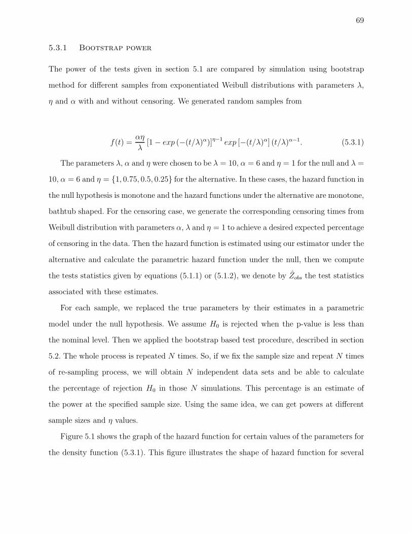
69
5.3.1 Bootstrap power
The power of the tests given in section 5.1 are compared by simulation using bootstrap
method for different samples from exponentiated Weibull distributions with parameters λ,
η and α with and without censoring. We generated random samples from
f(t) =αη
λ[1 − exp (−(t/λ)α)]η−1 exp [−(t/λ)α] (t/λ)α−1. (5.3.1)
The parameters λ, α and η were chosen to be λ = 10, α = 6 and η = 1 for the null and λ =
10, α = 6 and η = 1, 0.75, 0.5, 0.25 for the alternative. In these cases, the hazard function in
the null hypothesis is monotone and the hazard functions under the alternative are monotone,
bathtub shaped. For the censoring case, we generate the corresponding censoring times from
Weibull distribution with parameters α, λ and η = 1 to achieve a desired expected percentage
of censoring in the data. Then the hazard function is estimated using our estimator under the
alternative and calculate the parametric hazard function under the null, then we compute
the tests statistics given by equations (5.1.1) or (5.1.2), we denote by Zobs the test statistics
associated with these estimates.
For each sample, we replaced the true parameters by their estimates in a parametric
model under the null hypothesis. We assume H0 is rejected when the p-value is less than
the nominal level. Then we applied the bootstrap based test procedure, described in section
5.2. The whole process is repeated N times. So, if we fix the sample size and repeat N times
of re-sampling process, we will obtain N independent data sets and be able to calculate
the percentage of rejection H0 in those N simulations. This percentage is an estimate of
the power at the specified sample size. Using the same idea, we can get powers at different
sample sizes and η values.
Figure 5.1 shows the graph of the hazard function for certain values of the parameters for
the density function (5.3.1). This figure illustrates the shape of hazard function for several
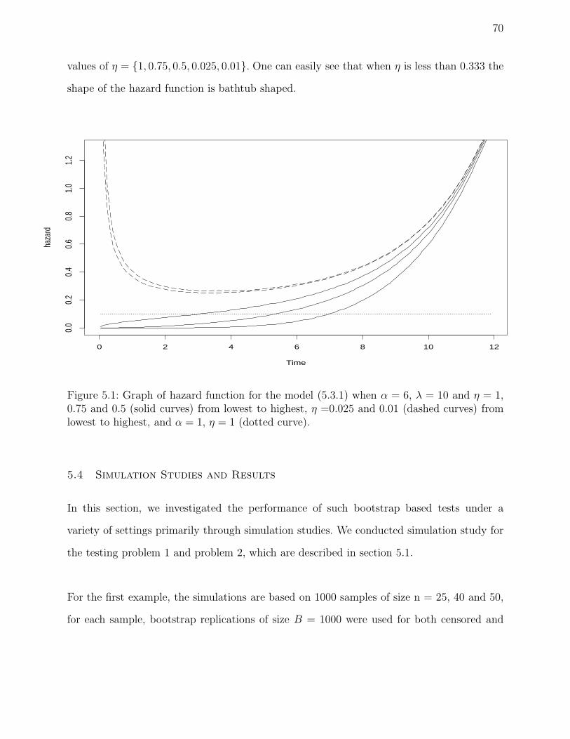
70
values of η = 1, 0.75, 0.5, 0.025, 0.01. One can easily see that when η is less than 0.333 the
shape of the hazard function is bathtub shaped.
Time
haza
rd
0 2 4 6 8 10 12
0.0
0.2
0.4
0.6
0.8
1.0
1.2
Figure 5.1: Graph of hazard function for the model (5.3.1) when α = 6, λ = 10 and η = 1,0.75 and 0.5 (solid curves) from lowest to highest, η =0.025 and 0.01 (dashed curves) fromlowest to highest, and α = 1, η = 1 (dotted curve).
5.4 Simulation Studies and Results
In this section, we investigated the performance of such bootstrap based tests under a
variety of settings primarily through simulation studies. We conducted simulation study for
the testing problem 1 and problem 2, which are described in section 5.1.
For the first example, the simulations are based on 1000 samples of size n = 25, 40 and 50,
for each sample, bootstrap replications of size B = 1000 were used for both censored and
71
uncensored samples. P-values estimation procedures with the scheme described in section 5.3
were carried out for N = 1000 Monte Carlo replications for each setting. Then the power was
computed by the proportion of rejection out of 1000 Monte-Carlo replications. The results
are displayed in Table 5.1. Power for the log rank (LR) and Kolmogorovs goodness-of-fit
(KS) under different alternatives is given as a function of η, based on the nominal levels
0.05. Note that η = 1 corresponds to the null hypothesis. From the results of Table 5.1 it can
easily be seen that the KS has higher power under the alternative than the LR in all cases
for both the censored and uncensored samples. When the parametric and shape restricted
hazard rates cross at some points, the log rank test may not have optimal power to detect
the difference in the hazard rates tests. Hence, this could be one of the possible reasons that
KS has higher power than LR under the alternative. In general, when the hazard rates are
proportional, the log-rank may have higher power to detect differences in the hazard rates.
For both tests the results clearly show that bootstrap power under the null is getting
closer and closer to the nominal size for the uncensored sample as n increases. On the other
hand, for small sample sizes under censoring the sizes of LR and KS are far from the margin
of the nominal level.
In the second example, we examine the power gains obtained by restricting the alternative
and looking at the power of a test of the hypothesis that the lifetimes come from a population
with a parametric hazard rate against a general not necessarily shape restricted alternative.
The tests statistic used for this purpose are the tests discussed in section 5.1 with slight
modification to log rank test as follows:
Z(τ) =D∑
i=1
W (ti)di
Y (ti)−∫ τ
0W (s)hpar(s)ds, (5.4.1)
where di is the number of events at the observed events times, t1, · · · , tD and Y (ti) is the
number of individuals under study just prior the observed event time ti. The quantity di
Y (ti)
72
gives a crude estimate of the hazard rate at an event time ti. As for the KS test we evaluated
the closeness of the Kaplan-Meier survival function estimator to the hypothesized S0(t).
To investigate the comparison, the power of the tests is computed numerically based on
the bootstrapped p-value for several choices of sample sizes n = 25, 50, 75, and 100. The
results are displayed in Table 5.2. In the first row of Table 5.2, LRSR and KSSR stands for
the log rank test and Kolmogorovs goodness of fit test computed under the shape restricted
alternative, respectively. Where as LRUR and KSUR represent both the tests computed under
a general not necessarily shape restricted alternative.
When the LR test statistic is used there is a sizable percentage in power gain under the
shape restricted alternative. Power gain using a shape restricted KS test was also observed in
all cases over a Kaplan-Meier based KS test although the extent was marginal. A plausible
explanation could be that the maximum difference between the estimated and the target
survival functions is achieved at a region that is relatively unaffected by the shape restriction
on the estimate. Also, the KS tests seem to have better power than the LR tests in this
example.
As n increase, the power increase as expected for all cases and the size of the test becomes
closer and closer to the nominal level under the null for both the shape restricted and unre-
stricted tests. For small sample the shape restricted test has better size than the unrestricted
test under the null.
Figure 5.2 shows power, as a function of η, for sample sizes 25, 50 and 100 based on 1000
replications and 1000 bootstrap samples for each replication. The power are constructed
using the log rank test statistic. From the graph we can see that the rejection probabilities
increase as the sample size increases as expected.
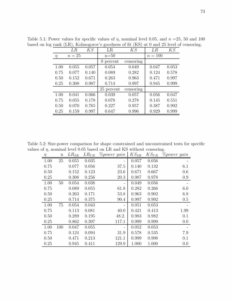
73
Table 5.1: Power values for specific values of η, nominal level 0.05, and n =25, 50 and 100based on log rank (LR), Kolmogorov’s goodness of fit (KS) at 0 and 25 level of censoring.
LR KS LR KS LR KSη n = 25 n=50 n = 100
0 percent censoring1.00 0.055 0.057 0.054 0.049 0.047 0.0530.75 0.077 0.140 0.089 0.282 0.124 0.5780.50 0.152 0.671 0.263 0.963 0.471 0.9970.25 0.308 0.987 0.714 0.997 0.945 0.999
25 percent censoring1.00 0.041 0.066 0.039 0.057 0.056 0.0470.75 0.055 0.178 0.078 0.278 0.145 0.5510.50 0.070 0.765 0.227 0.957 0.387 0.9920.25 0.159 0.997 0.647 0.996 0.929 0.999
Table 5.2: Size-power comparison for shape constrained and unconstrained tests for specificvalues of η, nominal level 0.05 based on LR and KS without censoring.
η n LRSR LRUR %power gain KSSR KSUR %power gain
1.00 25 0.055 0.035 - 0.057 0.056 -0.75 0.077 0.056 37.5 0.140 0.132 6.10.50 0.152 0.123 23.6 0.671 0.667 0.60.25 0.308 0.256 20.3 0.987 0.978 0.91.00 50 0.054 0.038 - 0.049 0.056 -0.75 0.089 0.055 61.8 0.282 0.266 6.00.50 0.263 0.171 53.8 0.963 0.902 6.80.25 0.714 0.375 90.4 0.997 0.992 0.51.00 75 0.054 0.043 - 0.051 0.053 -0.75 0.113 0.081 40.0 0.421 0.413 1.990.50 0.289 0.195 48.2. 0.983 0.982 0.10.25 0.862 0.397 117.1 0.999 0.999 0.01.00 100 0.047 0.055 - 0.052 0.053 -0.75 0.124 0.094 31.9 0.578 0.535 7.90.50 0.471 0.213 121.1 0.999 0.998 0.10.25 0.945 0.411 129.9 1.000 1.000 0.0
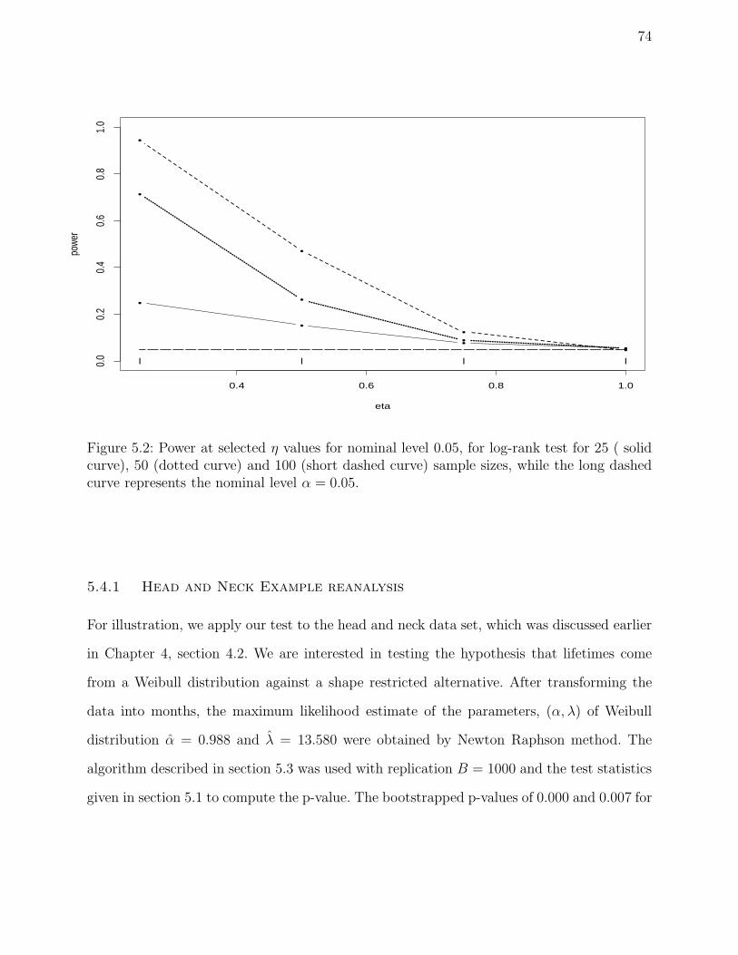
74
••
•
•
eta
powe
r
0.4 0.6 0.8 1.0
0.0
0.2
0.4
0.6
0.8
1.0
••
•
•
•
•
•
•
llll
Figure 5.2: Power at selected η values for nominal level 0.05, for log-rank test for 25 ( solidcurve), 50 (dotted curve) and 100 (short dashed curve) sample sizes, while the long dashedcurve represents the nominal level α = 0.05.
5.4.1 Head and Neck Example reanalysis
For illustration, we apply our test to the head and neck data set, which was discussed earlier
in Chapter 4, section 4.2. We are interested in testing the hypothesis that lifetimes come
from a Weibull distribution against a shape restricted alternative. After transforming the
data into months, the maximum likelihood estimate of the parameters, (α, λ) of Weibull
distribution α = 0.988 and λ = 13.580 were obtained by Newton Raphson method. The
algorithm described in section 5.3 was used with replication B = 1000 and the test statistics
given in section 5.1 to compute the p-value. The bootstrapped p-values of 0.000 and 0.007 for
75
the LR and KS were obtained. Thus, the null hypothesis that the lifetimes can be modeled
by Weibull distribution was rejected at 0.05 significance level. The p-values suggested the
inadequacy of the Weibull fit, which supports that the Weibull distribution is not appropriate
when the shape of the hazard function is not monotone.
5.4.2 Fan Generators Example
For our second example, we apply our tests to the fan generators data set which can be
found in Therneau and Grambsch (2000, p. 8). This data set originally appeared in Nelson
(1969). The data came from a field engineering study of the time to failure of diesel generator
fans. The data are replicated in Table D.1. The ultimate goal was to decide whether or not
to replace the working fans with a higher quality fan to prevent future failures. Seventy
generators were studied. For each generator, the number of hours of running time from first
being put into service until fan failure or until the end of the study (whichever came first)
was recorded. In this data set there were 11 uncensored and 59 censored observations. From
the data set the parameters of the hazard function under the null hypothesis were estimated
and the values of α = 1.059 and λ = 262.968 were obtained.
We assume that this data set has a decreasing convex hazard, since the engineering
problem was to determine whether the failure rate was decreasing over time (see Therneau
and Grambsch, 2000, p. 8). It was possible that the intial failures removed the weaker fans,
and the failure rate on the remaining fans would be tolerably low.
We use the bootstrap based p-value method with replication B = 1000 to test the hypoth-
esis that the data comes from a Weibull distribution. All the tests gave very high p-values,
LR (0.923) and KS (0.957) for testing the null hypothesis. We conclude that the data can
be modeled by a Weibull distribution with a constant hazard function.
76
5.4.3 Bone Marrow Transplantation for Leukemia Data Example revised
In chapter 4 we have estimated the hazard function based on bone marrow transplant for
leukemia using our method and other estimators. In this example, our main interest is to see if
the data can be modeled by parametric hazard function against shape restricted alternative.
From the data set the parameters of the hazard function under the null hypothesis were
estimated and the values of α = 0.658 and λ = 1097.514 were obtained. Now based on
bootstrapped p-value we found that the p-values of LR and KS equal to 0.190 and 0.658,
respectively. From these results, we can not reject the null hypothesis that the hazard function
can be modeled by a Weibull distribution with a decreasing hazard rate.
Chapter 6
CONCLUSIONS AND FUTURE RESEARCH
6.1 Summary
In this dissertation, we have introduced the nonparametric method for estimation of the
hazard or survival function when shape restrictions are imposed on the hazard function for
uncensored and right censored data.
The results from the simulation and real data set demonstrate the flexibility and prac-
ticality of the our estimator. The benefit of the shape restricted approach is that it can be
used to model any lifetime data whose shape is known, while parametric approach requires
complete knowledge of the underlying hazard function.
Although other nonparametric methods, such as kernel, Kaplan Meier and other methods
can be applied to estimate the hazard function or survival function, they might waste some
important information about the true underlying hazard function. Besides, the nonpara-
metric method may require user-defined parameters such as bandwidth. Hence, when the
only available information is that the underlying hazard function is decreasing, increasing,
concave, convex or bathtub-shaped, then the shape restricted method provide a more accept-
able estimate.
6.2 Bayesian Approach To Shape Restricted Hazard Function
A shape constrained maximum likelihood estimation may not be easily interpreted because
it is not smooth. In this work we suggest to use Bayesian approach with prior to the shape
77

78
restricted hazard function to serve as a smoothing technique. Then we will investigate the
estimation of hazard function and the related hypothesis tests.
Before going into the methods of finding Bayesian tests, we first discuss the Bayesian
approach to statistics. In the classical approach, the parameter (θ) is thought to be an
unknown, but fixed quantity. A random sample t1, . . . , tn is drawn from a population indexed
by θ and, based on the observed values in the sample, knowledge about the values of θ
is obtained. In the Bayesian approach, θ is considered to be a quantity whose variation
can be described by a probability distribution (called the prior distribution). A sample
t1, . . . , tn is then taken from a population indexed by θ and the prior distribution is updated
with this sample information. The updated prior is called the posterior distribution. This
updating is done using Bayes’s rule. All the inferences about θ are now based on the posterior
distribution.
Prior Distributions In order to use Bayesian approach in our case, we will apply priors
over all the unknown parameters. The unknown parameters in the shape restricted model
are the coefficients of the edge vectors and the coefficients of linear vectors. For example if
we consider convex constraint,
θ =n−2∑
j=1
bjδj + c1ν1 + c2ν2,
where bj ≥ 0, j = 1, · · · , n − 2; c1 and c2 are any real numbers.
Meyer and Laud (2005), and Jiang (2005) addressed the problem of incorporating prior
information into the unknown parameters in the shape restricted model. Following their
procedure, we will assign a gamma prior to the coefficients of the edge vectors. This is
because the coefficients need to be non-negative.
We will apply normal distribution priors with means µ1, µ2 and variances M1, M2 on the
linear coefficients c1, c2. The normal prior is suitable for the linear coefficients because it can
take any real values.

79
Selection of the prior parameters can be difficult. Jiang (2005) discussed some ways
of choosing prior parameters. In this work, we will extend the methods of choosing prior
parameters and will derive the posterior distribution. Based on the posterior distribution,
the hazard function will be estimated. Most of the posterior density is complicated, as it
is difficult to get it directly. However, numerical techniques such as Gibbs sampling will be
used to alleviate this difficulty.
6.3 Marginal Estimation of Hazard Function Under Shape Restriction in
Presence of Dependent Censoring
A crucial assumption in the construction of our likelihood function was that censoring
was independent of failure. Although this is a standard and classical assumption in the
vast majority of right censoring literature, it is still less than desirable for certain applica-
tions. Dependent censoring can occur if, for example, there are covariates affecting both the
censoring and failure time distributions. Such covariates could be both internal as well as
external. In a sense the situation with internal covariates is more crucial since they are no
ways to avoid them in some situation. A simple example can be considered to demonstrate
this. Consider individuals moving through successions of stages 1, 2 and 3 and let’s say we
are interested in estimating the waiting time distribution in stage 2. In the presence of right
censoring by a variable C, one has induced dependent censoring for the stage 1 waiting time
even if C was completely independent of the stage mechanisms.
If one could measure the covariates responsible for dependent censoring then there are
ways of accounting for them in the construction of marginal hazard rate function. We plan
to pursue this along with our shape restricted inference. This is easily accomplished via
the weighted approach. Basically, one needs to model the censoring hazard in terms of the
covariates inducing dependent censoring. In all the formulas before K needs to be replaced
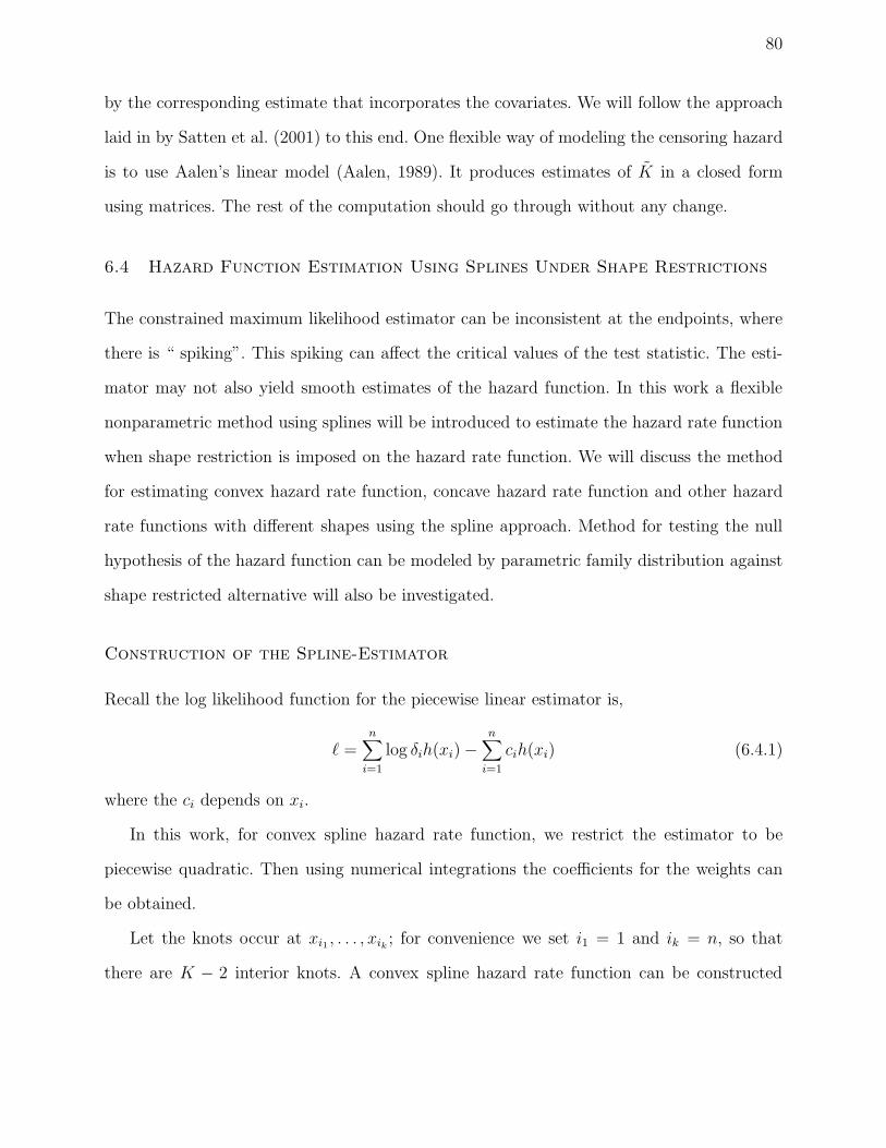
80
by the corresponding estimate that incorporates the covariates. We will follow the approach
laid in by Satten et al. (2001) to this end. One flexible way of modeling the censoring hazard
is to use Aalen’s linear model (Aalen, 1989). It produces estimates of K in a closed form
using matrices. The rest of the computation should go through without any change.
6.4 Hazard Function Estimation Using Splines Under Shape Restrictions
The constrained maximum likelihood estimator can be inconsistent at the endpoints, where
there is “ spiking”. This spiking can affect the critical values of the test statistic. The esti-
mator may not also yield smooth estimates of the hazard function. In this work a flexible
nonparametric method using splines will be introduced to estimate the hazard rate function
when shape restriction is imposed on the hazard rate function. We will discuss the method
for estimating convex hazard rate function, concave hazard rate function and other hazard
rate functions with different shapes using the spline approach. Method for testing the null
hypothesis of the hazard function can be modeled by parametric family distribution against
shape restricted alternative will also be investigated.
Construction of the Spline-Estimator
Recall the log likelihood function for the piecewise linear estimator is,
ℓ =n∑
i=1
log δih(xi) −n∑
i=1
cih(xi) (6.4.1)
where the ci depends on xi.
In this work, for convex spline hazard rate function, we restrict the estimator to be
piecewise quadratic. Then using numerical integrations the coefficients for the weights can
be obtained.
Let the knots occur at xi1 , . . . , xik ; for convenience we set i1 = 1 and ik = n, so that
there are K − 2 interior knots. A convex spline hazard rate function can be constructed
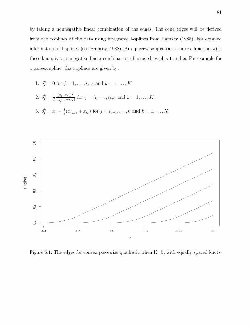
81
by taking a nonnegative linear combination of the edges. The cone edges will be derived
from the c-splines at the data using integrated I-splines from Ramsay (1988). For detailed
information of I-splines (see Ramsay, 1988). Any piecewise quadratic convex function with
these knots is a nonnegative linear combination of cone edges plus 1 and x. For example for
a convex spline, the c-splines are given by:
1. δkj = 0 for j = 1, . . . , ik−1 and k = 1, . . . , K.
2. δkj = 1
2
(xj−xik)2
(xik+1−xik
)for j = ik, . . . , ik+1 and k = 1, . . . , K.
3. δkj = xj −
12(xik+1
+ xik) for j = ik+1, . . . , n and k = 1, . . . , K.
t
c−sp
lines
0.0 0.2 0.4 0.6 0.8 1.0
0.0
0.2
0.4
0.6
0.8
1.0
Figure 6.1: The edges for convex piecewise quadratic when K=5, with equally spaced knots.
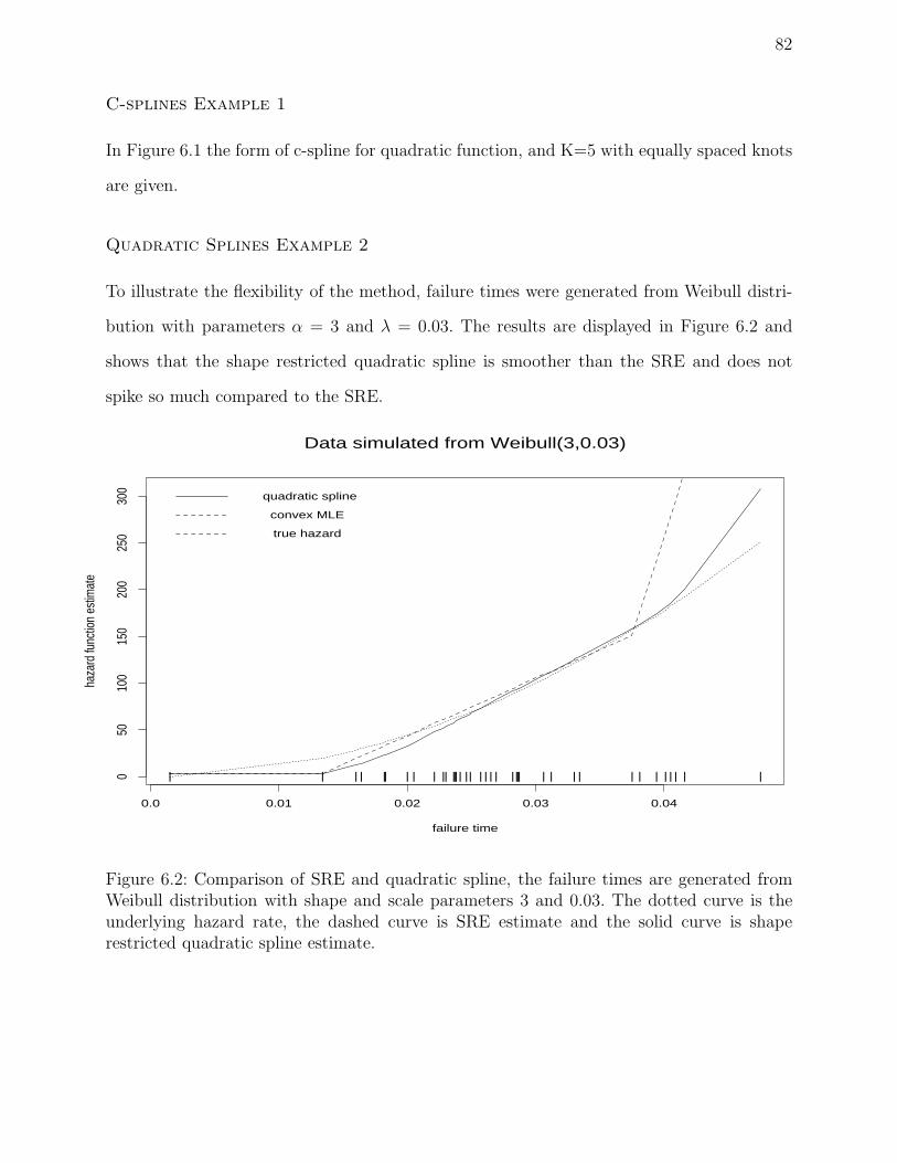
82
C-splines Example 1
In Figure 6.1 the form of c-spline for quadratic function, and K=5 with equally spaced knots
are given.
Quadratic Splines Example 2
To illustrate the flexibility of the method, failure times were generated from Weibull distri-
bution with parameters α = 3 and λ = 0.03. The results are displayed in Figure 6.2 and
shows that the shape restricted quadratic spline is smoother than the SRE and does not
spike so much compared to the SRE.
failure time
haza
rd fu
nctio
n es
timat
e
0.0 0.01 0.02 0.03 0.04
050
100
150
200
250
300
| | | | || | | | || |||| || | | | | |||| | | | | | | | | | | | |
quadratic spline
convex MLE
true hazard
Data simulated from Weibull(3,0.03)
Figure 6.2: Comparison of SRE and quadratic spline, the failure times are generated fromWeibull distribution with shape and scale parameters 3 and 0.03. The dotted curve is theunderlying hazard rate, the dashed curve is SRE estimate and the solid curve is shaperestricted quadratic spline estimate.
Bibliography
[1] Aalen, O. O. (1978). Nonparametric inference for family of counting process, The Annals
of Statistics, 6,, 701-726.
[2] Aalen, O. O. (1989). A linear regression model for the analysis of lifetimes, Statistics in
Medicine, 6, 907-925.
[3] Bickel, P.J, and Doksum, K.A. (1969). Tests for monotone failure rate based on nor-
malized spacings, The Annals of Mathematical Statistics, 40, 1216-1235.
[4] Bickel, P. and Rosenblatt, M. (1973). On some global measures of the deviations of
density function estimates, The Annals of Statistics, 1, 1071 1095.
[5] Barlow, R.E, and Proschan, F. (1969). A note on tests for monotone failure rate based
on incomplete data, The Annals of Mathematical Statistics, 40, 595-600.
[6] Carlin B. P. and Polson N. G. (1991). Inference for nonconjugate Bayesian models using
the Gibbs sampler, Canadian Journal of Statistics, 19, 399-405.
[7] Cox, D. R. (1972). Regression models and life tables, Journal of the Royal Statistical
Society, 34, 187-220.
[8] Davison, R. and MacKinnon, J. G. (1998). Graphical methods for investigating the size
and power hypothesis tests, The Manchester School, 66, 1-26.
[9] Efron, B. (1981). Bootstrap methods: Another look at the Jackknife, Annals of Statis-
tics, 7, 1-26.
83
84
[10] Efron, B. (1981). Censored data and bootstrap, Journal of the American Statistical
Association, 76, 312-319.
[11] Efron, B. (1987). Better bootstrap confidence intervals, Journal of the American Sta-
tistical Association, 82, 171-200.
[12] Efron, B. (1988). Logistic regression, survival analysis, and the Kaplan-Meier Curve,
Journal of the American Statistical Association, 83, 414-425.
[13] Efron, B. and Tibshirani, R. (1986). Bootstrap method for standard errors, confidence
intervals, and other measures of statistical accuracy, Statistical Science, 1, 54-75.
[14] Epanechnikov, V.A. (1969). Nonparametric estimation of a multidimensional probability
density, Theory of Probability and its Applications, 14, 153-158.
[15] Gerlach, B. (1987). Testing exponentially against increasing failure rate with randomly
censored data, Statistics, 18, 268-275.
[16] Fleming, T.R, and Harrington, D.P. (1991). Counting Processes and Survival Analysis,
Wiley, New York.
[17] Florenzano, M., and Le Van, C. (2001). Finite Dimensional Convexity and Optimization,
Springer- Verlag Berlin, Germany.
[18] Fraser, D.A.S. and Massam, H. (1989). A mixed primal-dual bases algorithm for
regression under inequality constraints, Application to convex regression, Scandinavian
Journal of Statistics, 16, 65-74.
[19] Gehan, E.A. (1965). A generalized Wilcoxon test for comparing arbitrarily singly-
censored samples, Biometrika, 52, 203-223.
85
[20] Gelfand, A. E, Hills, S. E., Racine-Poon, A., Smith, A. F. M. (1990). Illustration of
Bayesian inference in normal data models using Gibbs sampler, Journal of the American
Statistical Association, 85, 972-985.
[21] Hall, P, and Heckman, N. (2000). Testing for monotonicity of a regression mean by
calibrating for linear functions, The Annals of Statistics, 28, 20-39.
[22] Hall, P, and Horrowitz, J. L. (1996). Bootstrap critical values for tests based on gener-
alized method of moments estimators, Econometrica, 64, 891-916.
[23] Hess, K. R, Serachitopol, D. M. and Brown, B. W. (1999). Hazard function estimation:
A simulation study, Statistics in Medicine, 18, 3075-3088.
[24] Kalbfleisch, J.D. and Prentice, R.L. (1980). The Statistical Analysis of Failure Time
Data, Wiley, New york.
[25] Kaplan, E.L, and Meier, P. (1958). Nonparametric Estimation from incomplete samples,
Journal of the American Statistical Association, 53, 457-481.
[26] Jiang, Yan. (2005). Semiparametric ancova using shape restrictions, Unpublished PhD
dissertation, University of Georgia, Athens, Georgia
[27] Klein, J. P, and Moeschberger, M. L. (1997). Survival Analysis: Techniques for Censored
and Truncated Data, Springer-Verlag, New York.
[28] Koul, H., Susarla,V., Van Ryzin, J. (1981). Regression analysis of randomly right-
censored data, Annals of Statistics, 9, 1276-1288.
[29] Kouassi, D. A, and Singh, J. M. (1997). A Semiparametric approach to hazard estima-
tion with randomly censored observations, Journal of the American Statistical Associ-
ation, 92, 1351-1355.
86
[30] Liu, R. Y. C and Van Ryzin, J. (1985). A Histogram estimator of the hazard rate with
censored data, Annals of Statistics, 13, 592-605.
[31] Meyer, M. C. (1999a). An extension of the mixed primal-dual bases algorithm to the
case of more constraints than dimensions, Journal of Statistical Planning and Inference,
81, 13-31.
[32] Meyer, M. C. (1999b). A comparison of nonparametric shape constrained bioassay esti-
mators, Statistics and Probability letters, 42, 267-274.
[33] Meyer, M. C. (2003). A test for linear versus convex regression function using shaped-
restricted regression, Biometrika, 90, 223-232.
[34] Meyer, M. C. (2006). Shape- Restricted Regression Splines, preprint.
[35] Meyer, M. C., and Lund, R. (2003). Inference in shape-restricted regression with time-
series data, preprint.
[36] Meyer, M. C., and Laud, P. W. (2005). A Bayesian approach to shape-restricted regres-
sion, Department of Statistics Technical Report, the University of Georgia.
[37] Meyer, M. C., and Woodroofe, M. (2004). Estimation of a unimodal density using shape
restrictions,Canadian Journal of Statistics, 32, 85-100.
[38] Miller, R. G. (1981). Survival Analysis, John Wiley & Sons, New York.
[39] Miller, R. G. (1983). What price Kaplan -Meier? Biometrika, 39, 1077-1081.
[40] Muller, H. G., and Wang, J.L. (1990). Nonparametric analysis of changes in hazard
rate with censored survival data: an alternative to change-point models, Biometrika, 7,
305-314.
87
[41] Mudholkar, G, Srivastava, D. K, and Freimer M. (1995). The exponentiated Weibull
family: A reanalysis of the bus-motor failure data, Technometrics, 4, 436-445.
[42] Proschan, F. and Pyke, R. (1967). Tests for monotone failure rate, Fifth Berkeley Sym-
posium, 3, 293-313.
[43] Peto, R. and Peto, J. (1972). Asymptotically efficient rank invariant test procedures,
Journal of the Royal Statistical Society, 135, 185-206.
[44] Ramlau-Hansen, H.(1983). Smoothing counting process intensities by means of kernel
functions, The Annals of Statistics, 11, 435-466.
[45] Ramsay, J. O. (1988). Monotone Regression Splines in action, Statistical Science, 3,
425-461.
[46] Robertson, T., Wright, F. T., and Dykstra, R. L. (1988). Order Restricted Statistical
Inference, John Wiley & Sons, New York.
[47] Rockafellar, R. T. (1970). Convex Analysis, Princeton University Press, New Jersey.
[48] Satten, G. A. and Datta, S (2000). The Kaplan-Meier Estimator as Inverse-Probability
-of Censoring Weighted Average, American Statistician, 81, 13-31.
[49] Satten, G. A., Datta, S, and J., Robins. (2001). Estimating the marginal survival func-
tion in the presence of time dependent covariates, Statistics and Probability letters, 54,
397-403.
[50] Silverman, B.W. (1986). Density Estimation for Statistics and Data Analysis, Chapman
and Hall, New York.
[51] Smith, P.J. (2002). Analysis of Failure and Survival Data, Chapman and Hall, Boca
Raton, Florida.
88
[52] Tanner, M. A.(1983). A note on the variable kernel estimator of the hazard function
from censored data, The Annals of Statistics, 11, 994-998.
[53] Tanner, M. A, and Wong, W, H. (1983). The estimation of the hazard function from
random censored data by kernel method, The Annals of Statistics, 11, 989-993.
[54] Therneau, T, and Grambsch, P. M. (2000). Modeling survival data : extending the Cox
model, Springer, New York.
[55] Watson, G.S, and Leadbetter, M. R. (1964a) Hazard analysis I, Biometrika, 51, 175-184.
[56] Watson, G.S, and Leadbetter, M. R. (1964b) Hazard analysis II, Sankhya, 26, 101-116.
[57] Wedman, E. J, and Wright, I. W. (1983). Splines in statistics, Journal of the American
Statistical Association, 78, 351-365.
[58] Xiong, J.P, Miller, F. G, and Yan, Y. (2004). Testing increasing hazard rate for progres-
sion time of dementia, Discrete and Continuous Dynamic Systems Series, 4, 813-821.

Appendix A
Head and Neck Cancer data for Arm A
The head and neck data set is from a clinical trial conducted by Northern Oncology Group,
discussed by Efron (1988). The data represent the survival times of 51 head and neck cancer
patients under treatment A, who were given radiation therapy. Nine patients were lost to
follow up and were considered as censored.
89
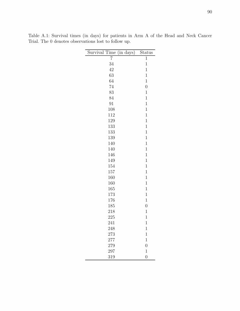
90
Table A.1: Survival times (in days) for patients in Arm A of the Head and Neck CancerTrial. The 0 denotes observations lost to follow up.
Survival Time (in days) Status7 134 142 163 164 174 083 184 191 1108 1112 1129 1133 1133 1139 1140 1140 1146 1149 1154 1157 1160 1160 1165 1173 1176 1185 0218 1225 1241 1248 1273 1277 1279 0297 1319 0
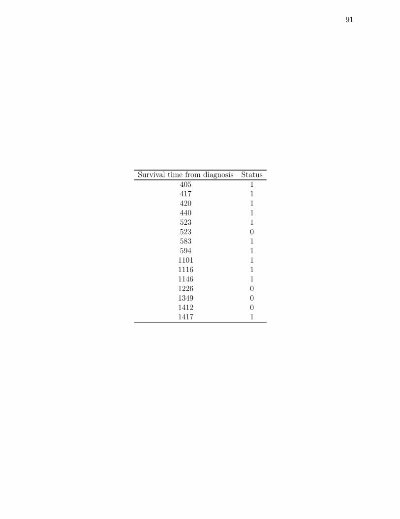
91
Survival time from diagnosis Status405 1417 1420 1440 1523 1523 0583 1594 11101 11116 11146 11226 01349 01412 01417 1
Appendix B
Bone Marrow Transplantation for leukemia data
Bone marrow transplant for leukemia data set is taken from Klein and Moeschberger (2003, p.
3). Out of their three sets of leukemia patient groups, we considered the patients in the group
with acute lymphoblastic leukemia (ALL). Transplantation is considered a failure when a
patient’s leukemia returns (relapse) or when he or she dies while in remission (treatment
related death). In this data set there were 23 uncensored and 14 censored observations.
92
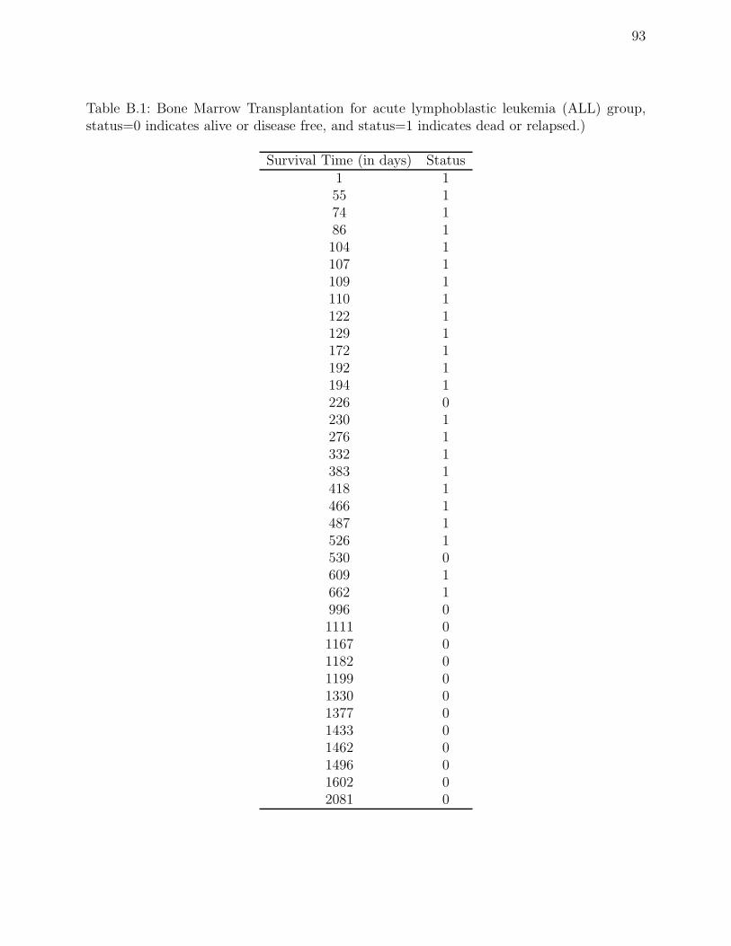
93
Table B.1: Bone Marrow Transplantation for acute lymphoblastic leukemia (ALL) group,status=0 indicates alive or disease free, and status=1 indicates dead or relapsed.)
Survival Time (in days) Status1 155 174 186 1104 1107 1109 1110 1122 1129 1172 1192 1194 1226 0230 1276 1332 1383 1418 1466 1487 1526 1530 0609 1662 1996 01111 01167 01182 01199 01330 01377 01433 01462 01496 01602 02081 0

Appendix C
Data for Leukemia Survival Patients
This data set is taken from Lee (1980, Table 3.3, p. 72). The data set was originally appeared
in Hart et al. (1977). Seventy-one adult patients with acute leukemia (ALL) and acute
myeloblastic Leukemia (AML) were studied at M.D. Anderson Hospital and Tumor Institute.
There were some covariates in the data set, in this study we consider the survival of the
patients from diagnosis of acute myeloblastic Leukemia (AML) and survival status (life or
death). There were 51 observations, of which 6 are censored.
94
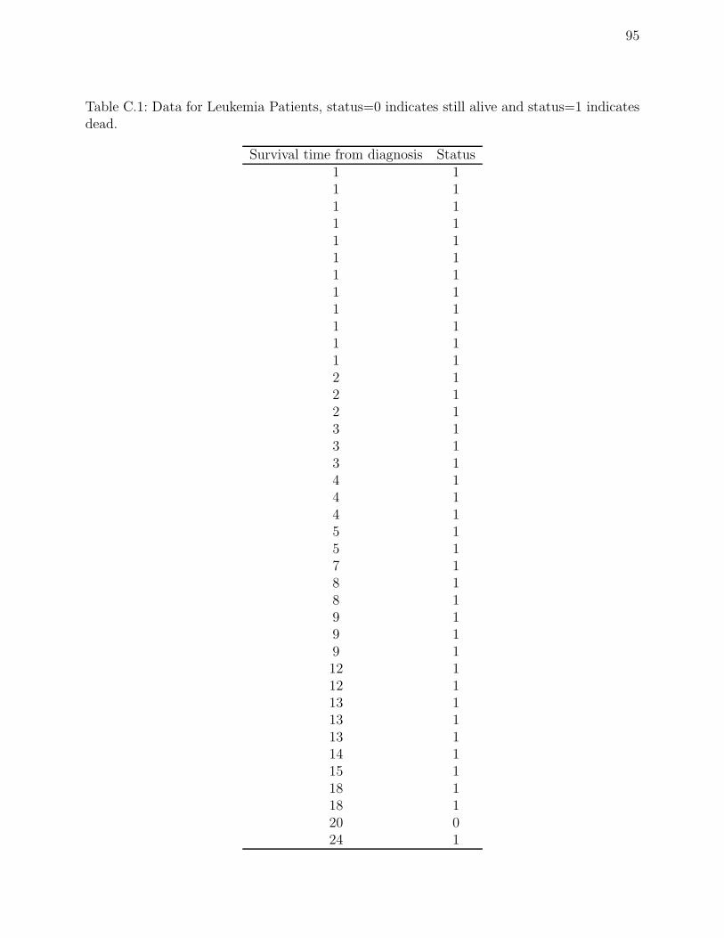
95
Table C.1: Data for Leukemia Patients, status=0 indicates still alive and status=1 indicatesdead.
Survival time from diagnosis Status1 11 11 11 11 11 11 11 11 11 11 11 12 12 12 13 13 13 14 14 14 15 15 17 18 18 19 19 19 112 112 113 113 113 114 115 118 118 120 024 1
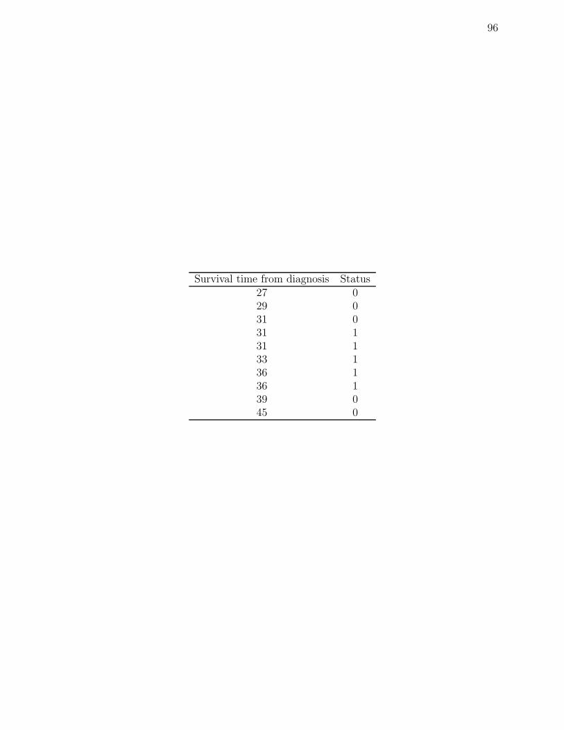
96
Survival time from diagnosis Status27 029 031 031 131 133 136 136 139 045 0

Appendix D
Generator fans failure data
This data set is found in Therneau and Grambsch (2000, p. 8); and Nelson (1969). The
data come from a field engineering study of the time to failure of diesel generator fans. The
ultimate goal was to decide whether or not to replace the working fans with a higher quality
fan to prevent future failures. Seventy generators were studied. For each one, the number of
hours of running time from its first being put into service until fan failure or until the end
of the study (whichever came first) was recorded. In this data set there were 11 uncensored
and 59 censored observations.
97
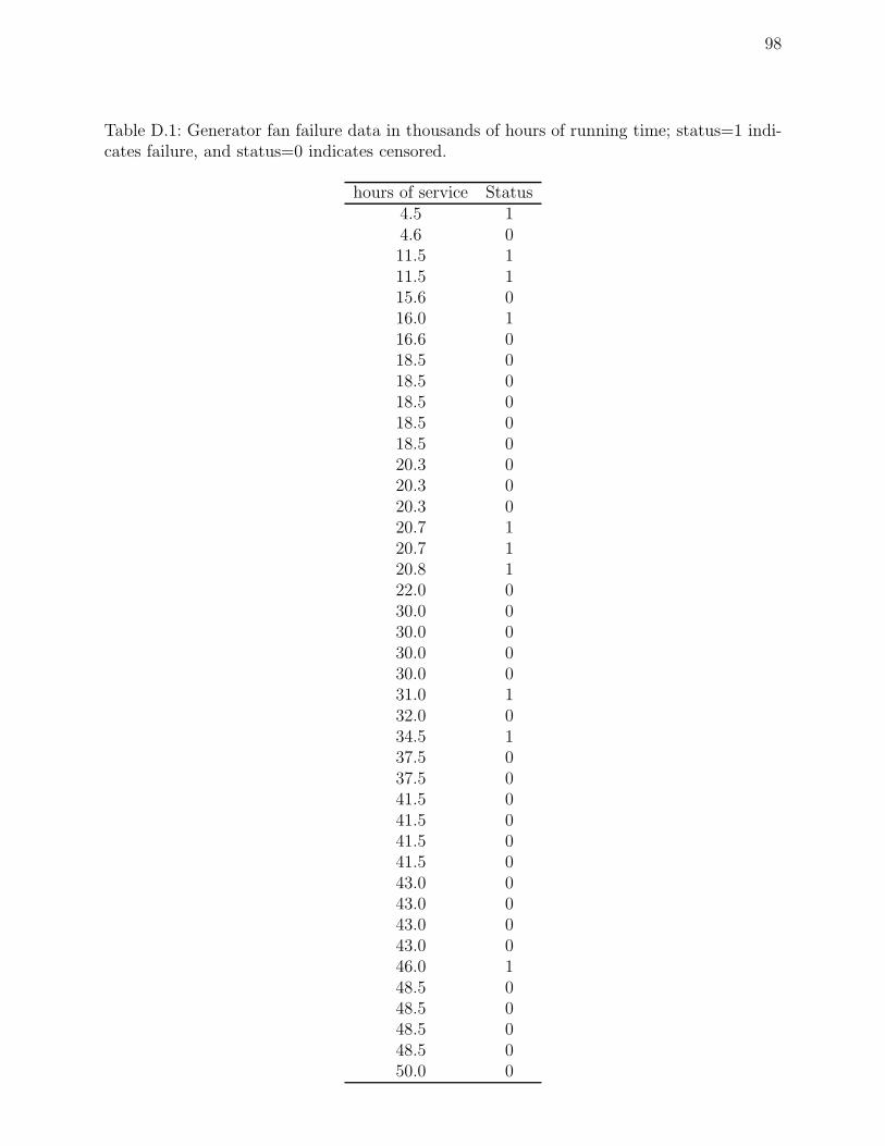
98
Table D.1: Generator fan failure data in thousands of hours of running time; status=1 indi-cates failure, and status=0 indicates censored.
hours of service Status4.5 14.6 011.5 111.5 115.6 016.0 116.6 018.5 018.5 018.5 018.5 018.5 020.3 020.3 020.3 020.7 120.7 120.8 122.0 030.0 030.0 030.0 030.0 031.0 132.0 034.5 137.5 037.5 041.5 041.5 041.5 041.5 043.0 043.0 043.0 043.0 046.0 148.5 048.5 048.5 048.5 050.0 0
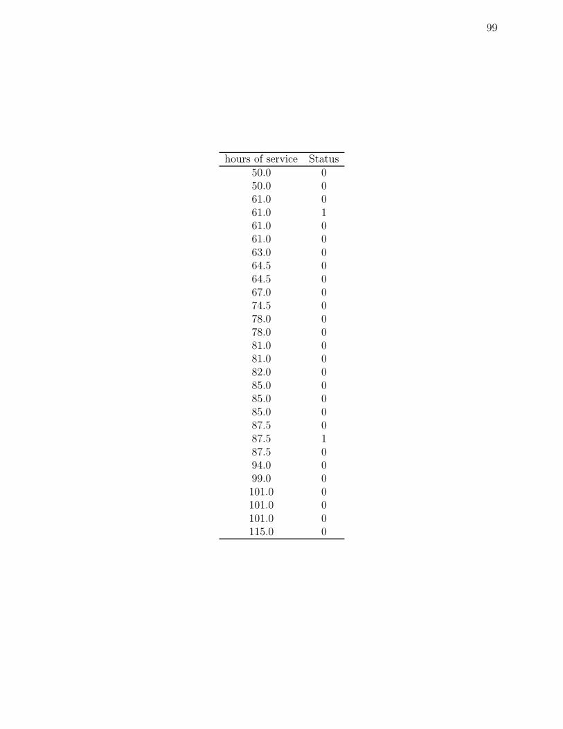
99
hours of service Status50.0 050.0 061.0 061.0 161.0 061.0 063.0 064.5 064.5 067.0 074.5 078.0 078.0 081.0 081.0 082.0 085.0 085.0 085.0 087.5 087.5 187.5 094.0 099.0 0101.0 0101.0 0101.0 0115.0 0