Maximum Likelihood Estimates of Regression

Coefficients with α-stable residuals and Day of Week

effects in Total Returns on Equity Indices

John C. Frain.∗

11th June 2006

Abstract

This Paper summarizes the theory of Maximum Likelihood Estimation of re-

gressions with α-stable residuals. Day of week effects in returns on equity indices,

adjusted for dividends (total returns) are estimated and tested using this and tra-

ditional OLS methodology. I find that the α-stable methodology is feasible. There

are some differences in the results from the two methodologies. The conclusion

remains that if individual coefficients are of interest and the residuals have fat tails

and a possible α-stable distribution, the results should be checked for robustness

using methods such as those employed here.

Contents

1 Introduction 2

2 Regression with non-normal α-Stable Errors 4

3 Maximum Likelihood Estimates of Day of Week Effects with α-Stable

errors 7

4 Summary and Conclusions 15

A An Introduction to α-Stable Processes 18

∗Comments are welcome. My email address is frainj@tcd.ie. This document is work in progress.

Please consult me before quoting. Thanks are due to Prof. Antoin Murphy and to Michael Harrison for

help and suggestions and to participants at a seminar in TCD for comments reseived. Any remaining

errors in the paper are my responsibility. I would also like to thank my wife, Helen, for her great support

and encouragement.

1

1 Introduction

Returns on many assets are known to have fat tails and are often skewed. The almost

universally used Normal or Gaussian distribution can model neither fat tails nor skew-

ness. The α stable distribution can model these features. The use of this distribution

in Finance was originally proposed by Mandelbrot (see Mandelbrot (1962, 1964, 1967)

or Mandelbrot and Hudson (2004)) to model vaious goods and asset prices. It became

popular in the sixties and seventies but interest waned thereafter. This decline in inter-

est was due not only to its mathematical complexity and the considerable computation

resources required but to the considerable success of the Merton Black Scholes Gaussian

approach to Finance theory which was developed at the same time.

Recently there has been some renewed interest in the distribution. Recent Mathematical

accounts are given in Zolotarev (1986), Samorodnitsky and Taqqu (1994), Weron (1998)

and Uchaikin and Zolotarev (1999). Rachev and Mittnik (2000) survey the use of α-

stable models in finance.

The availability of cheap powerful computer hardware has made advanced computation

resources available to scientists in many fields. The resulting increased demand for good

software has provided the incentive to produce and distribute widely software pack-

ages such as Mathematica (Wolfram (2003)) and R (R Development Core Team (2006))

which have facilitated the calculations in this paper. Programs in to compute α-stable

distribution and density functions are available in both of these packages (Mathemat-

ica (Rimmer (2005)), Rmetrics for R (Wuertz (2005)) or as the stand-alone program

STABLE (Nolan (2005))). These resources allow one to examine the consequences of

replacing the Normal assumption with the more general α-stable. Further advances in

theory and computation facilities will facilitate this process in the coming years and the

use of the α-stable distribution will become more common.

In particular, this paper examines the consequences of α-stable residuals in OLS esti-

mation. In section (2) the following results are set out:

• Standard OLS Estimates are consistent but inefficient.

• Coefficient Estimates have an α-stable distribution and standard t-statistics do

not have the usual distribution

• Maximum Likelihood estimation have the usual asymptotic properties of Maximum

Likelihood estimators and confidence intervals and inference may be based on the

usual maximum likelihood theory.

• Maximum Likelihood estimation with α-stable residuals is a form of robust esti-

mator which gives less weight to extreme observations

In section (3) this theory is applied to estimating and testing calendar effects in daily re-

turns on equity indices. These day-of-week effects are often estimated by the coefficients

2

in an OLS regression of daily returns on five dummy variables - one for each day of the

week. I compare the results estimating of estimating such regressions using standard

OLS and and α-stable maximum likelihood. Estimates are made for six total returns

indices (ISEQ, CAC40, DAX30, FTSE100, Dow Jones Composite (DJC) and S&P500)

and the DJIA for the period used in the often quoted study of these effects in Gibbons

and Hess (1981). My results can be summarized as follows -

• The α-stable maximum likelihood and OLS estimates for the DJIA for the Gibbons

and Hess (1981) are almost identical.

• Data for the total returns indices are only available from the late 1980’s (apart

from the DAX30) and there are no significant week-day effects in the total returns

indices in that period

• When the data for the CAC40 are split into three equal periods there are indica-

tions of weekday effects in the two early periods but they are absent in the late

period.

These results are a demonstration of the shifting Monday effect reported in the literature

(see Pettengill (2003) and the references there and Hansen et al. (2005)). Such results

are, therefore, not sensitive to the use of the “robust” α-stable Maximum Likelihood

Estimator.

An examination of the significance of the results for individual coefficients shows that

some α-stable coefficients are significant where the corresponding OLS are not. Sullivan

et al. (2001) sets out the danger of data mining in cases such as this. I would not draw

any conclusions about weekday effects from these discrepancies. They do, however,

draw attention to the possible different results that may arise from α-stable maximum

likelihood estimation.

3

2 Regression with non-normal α-Stable Errors

Consider the standard regression model

yi =

k∑

j=1

xijβj + εi, i = 1, . . . , N (1)

where yi is an observed dependent variable, the xij are observed independent variables,

βj are unknown coefficients to be estimated and εi are identically and independently

distributed. Equation 1 may be written in matrix form as

y = Xβ + ε (2)

where

y =

y1

y2

...

yN

,X =

x11 x12 . . . x1k

x21 x22 . . . x2k

......

. . ....

xN1 xN2 . . . xNk

,β =

β1

β2

...

βk

, ε =

ε1

ε2

...

εN

(3)

The standard OLS estimator of β is

βOLS = (X′X)−1X′y (4)

Thus

βOLS − β = (X′X)−1X′ε (5)

Thus in the simplest case where X is predetermined βOLS − β is a linear sum of the

elements of ε. If the elements of ε are independent identically distributed non-normal

α-stable variables then βOLS has an α-stable distribution. The variance of εi does not

even exist. Thus standard OLS inferences are not valid. (Logan et al. (1973)) prove the

following properties of the asymptotic t-statistic

1. The tails of the distribution function are normal-like at ±∞

2. The density has infinite singularities |1 ∓ x|−α at ±1 for 0 < α < 1 and β 6= ±1.

When 1 < α < 2 the distribution has peaks at ±1.

3. As α → 2 the density tends to normal and the peaks vanish

When 1 < α < 2 the OLS estimates are consistent but converge ar a rate of n1

α−1 rather

than n− 1

2 in the normal case.

DuMouchel (1971, 1973, 1975) shows that, subject to certain conditions, the maximum

likelihood estimates of the parameters of an α-stable distribution have the usual asymp-

totic properties of a Maximum Likelihood estimator. They are asymptotically normal,

asymptotically unbiased and have an asymptotic covariance matrix n−1I(α, β, γ, δ)−1

4

where I(α, β, γ, δ) is Fisher’s Information. McCulloch (1998) examines linear regression

in the context of α-stable distributions paying particular attention to the symmetric

case. Here the symmetry constraint is not imposed. Assume that εi = yi −∑k

j=1 xijβj

is α-stable with parameters {α, β, γ, 0}. If we denote the α-stable density function by

s(x, α, β, γ, δ) then we may write the density function of εi as

s(εi, α, β, γ, δ) =1

γs

(

yi −∑k

j=1 xijβj

γ, β, 1, 0

)

, (6)

the Likelihood as

L(ε, α, β, γ, β1, β2, . . . ) =

(

1

γ

)n n∏

i=1

s

(

yi −∑k

j=1 xijβj

γ, β, 1, 0

)

, (7)

and the Loglikelihood as

l(ε, α, β, γ, β1, β2, . . . ) =

n∑

i=1

(

−n log(γ) + log

(

s

(

yi −∑k

j=1 xijβj

γ, β, 1, 0

)))

=n∑

i=1

φ(εi).

(8)

The maximum likelihood estimators are the solutions of the equations

∂l

∂βm=

n∑

i=1

−φ′(εi)xim = 0, m = 1, 2, . . . , k

n∑

i=1

−φ′(εi)

εiεixim = 0, m = 1, 2, . . . , k

n∑

i=1

−φ′(εi)

εi(y1 −

k∑

j=1

xijβj)xim = 0, m = 1, 2, . . . , k

n∑

i=1

−φ′(εi)

εi(yi −

k∑

j=1

xijβj)xim = 0, m = 1, 2, . . . , k

n∑

i=1

−φ′(εi)

εiyixim =

n∑

i=1

−φ′(εi)

εi

k∑

j=1

xijβj

(9)

If W is the diagonal matrix

W =

−φ′(ε1)ε1

0 . . . 0

0 −φ′(ε2)ε2

. . . 0...

.... . .

...

0 0 . . . −φ′(εn)εn

, (10)

Using the notation in equation (3)we may write equation (9) in matrix format.

X ′Wy = (X ′WX)β (11)

5

or if X ′WX is not singular

β = (X ′WX)−1X ′Wy (12)

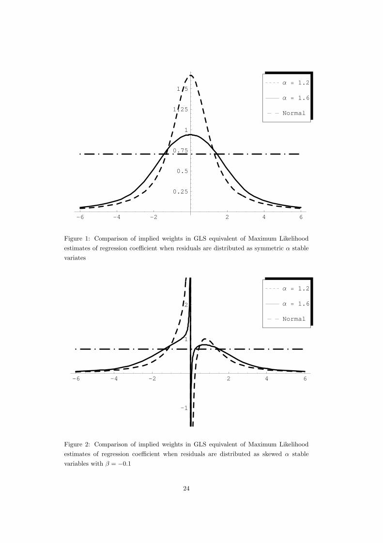
Thus the maximum likelihood regression estimator has the format of a Generalized

Least Squares estimator in the presence of heteroscedasticity where the variance1 of the

error term εi is proportional to φ′(εi)εi

. The effect of the “Generalized Least Squares”

adjustment is to give less weight to larger observations. Figure 1 compares the weighting

pattern derived from equation (10) for α-stable processes with α = 1.2 and 1.6 with those

of a standard normal distribution. For compatibility purposes the α-stable curves are

drawn with γ = 1/√

2. As expected the normal distribution gives equal weights to all

observations. The estimator for α-stable processes gives higher weights to the center of

the distribution and extremely small weights to extreme values. This effect increases as

α is reduced.

This result explains the results obtained by Fama and Roll (1968) who completed a

Monte Carlo study of the use of truncated means as measures of location in α-stable

distributions. They found

When α = 1.1 the .25 truncated2 means are still dominant for all n. For α =

1.3 and α = 1.5 the .50 truncated means are generally best, and when α = 1.9

the distributions of the .75 truncated means are uniformly less disperse than

those of other estimators. Finally, when the generating process is Gaussian

(α = 2) the mean is the “best” estimator. Of course it is also minimum-

variance, unbiased in this case.

The shape of the weight curves in the skewed case is shown in figure (2). The weights

are based on the same α-stable distributions as those in figure 1 except that β is now

−0.1. The most surprising aspect of the weighting systems is the negative weights given

to small positive observations. Again the effects are more pronounces as α is reduced.

1This is only an analogy. The vatiance of the error term does not exist2A g truncated mean retains 100g% of the data. Thus a .25 truncated mean is an average of the

central 25% of the data

6

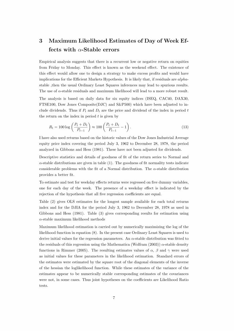
3 Maximum Likelihood Estimates of Day of Week Ef-

fects with α-Stable errors

Empirical analysis suggests that there is a recurrent low or negative return on equities

from Friday to Monday. This effect is known as the weekend effect. The existence of

this effect would allow one to design a strategy to make excess profits and would have

implications for the Efficient Markets Hypothesis. It is likely that, if residuals are alpha-

stable ,then the usual Ordinary Least Squares inferences may lead to spurious results.

The use of α-stable residuals and maximum likelihood will lead to a more robust result.

The analysis is based on daily data for six equity indices (ISEQ, CAC40, DAX30,

FTSE100, Dow Jones Composite(DJC) and S&P500) which have been adjusted to in-

clude dividends. Thus if Pt and Dt are the price and dividend of the index in period t

the return on the index in period t is given by

Rt = 100 log

(

Pt + Dt

Pt−1

)

≈ 100

(

Pt + Dt

Pt−1− 1

)

. (13)

I have also used returns based on the historic values of the Dow Jones Industrial Average

equity price index covering the period July 3, 1962 to December 28, 1978, the period

analyzed in Gibbons and Hess (1981). These have not been adjusted for dividends.

Descriptive statistics and details of goodness of fit of the return series to Normal and

α-stable distributions are given in table (1). The goodness of fit normality tests indicate

considerable problems with the fit of a Normal distribution. The α-stable distribution

provides a better fit.

To estimate and test for weekday effects returns were regressed on five dummy variables,

one for each day of the week. The presence of a weekday effect is indicated by the

rejection of the hypothesis that all five regression coefficients are equal.

Table (2) gives OLS estimates for the longest sample available for each total returns

index and for the DJIA for the period July 3, 1962 to December 28, 1978 as used in

Gibbons and Hess (1981). Table (3) gives corresponding results for estimation using

α-stable maximum likelihood methods

Maximum likelihood estimation is carried out by numerically maximizing the log of the

likelihood function in equation (8). In the present case Ordinary Least Squares is used to

derive initial values for the regression parameters. An α-stable distribution was fitted to

the residuals of this regression using the Mathematica (Wolfram (2003)) α-stable density

functions in Rimmer (2005). The resulting estimates values of α, β and γ were used

as initial values for these parameters in the likelihood estimation. Standard errors of

the estimates were estimated by the square root of the diagonal elements of the inverse

of the hessian the loglikelihood function. While these estimates of the variance of the

estimates appear to be numerically stable corresponding estimates of the covariances

were not, in some cases. Thus joint hypotheses on the coefficients are Likelihood Ratio

tests.

7

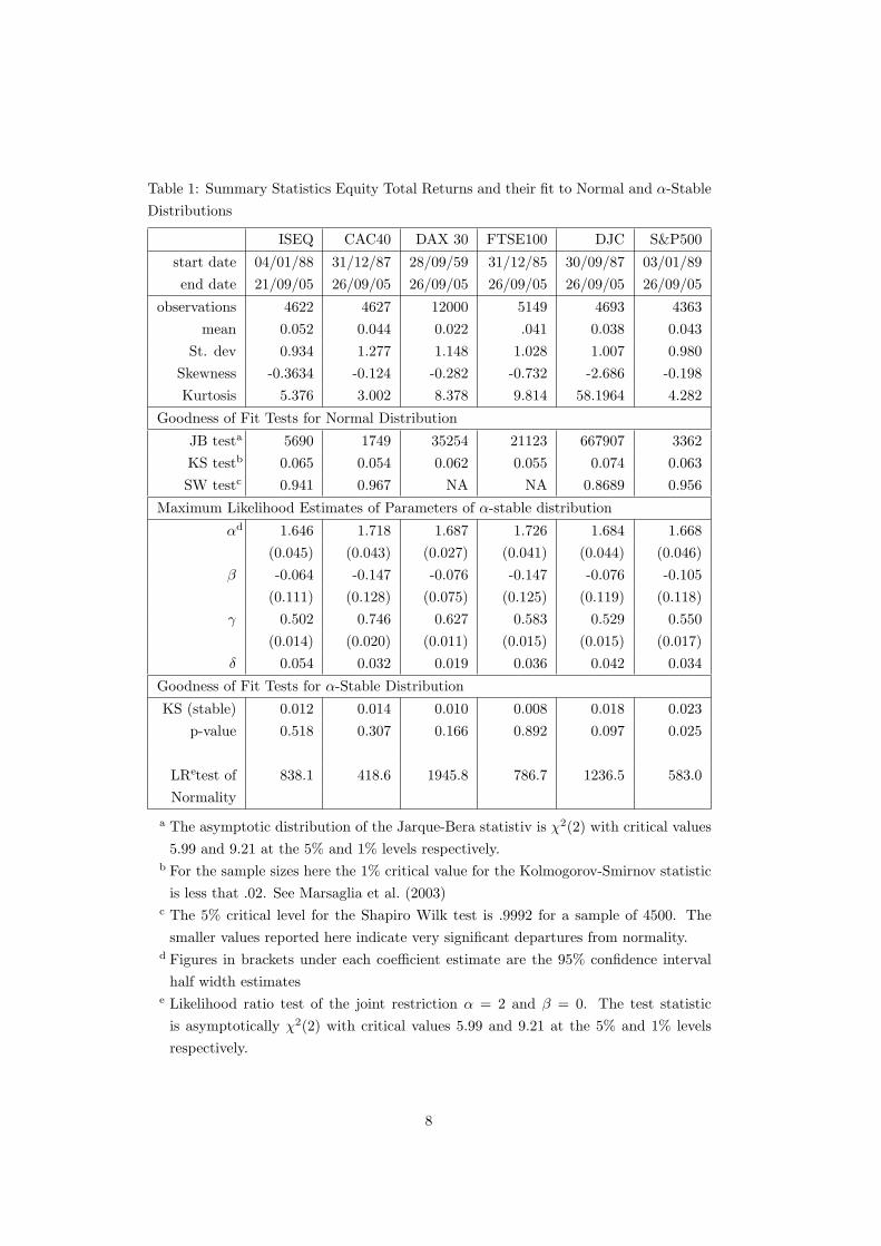
Table 1: Summary Statistics Equity Total Returns and their fit to Normal and α-Stable

Distributions

ISEQ CAC40 DAX 30 FTSE100 DJC S&P500

start date 04/01/88 31/12/87 28/09/59 31/12/85 30/09/87 03/01/89

end date 21/09/05 26/09/05 26/09/05 26/09/05 26/09/05 26/09/05

observations 4622 4627 12000 5149 4693 4363

mean 0.052 0.044 0.022 .041 0.038 0.043

St. dev 0.934 1.277 1.148 1.028 1.007 0.980

Skewness -0.3634 -0.124 -0.282 -0.732 -2.686 -0.198

Kurtosis 5.376 3.002 8.378 9.814 58.1964 4.282

Goodness of Fit Tests for Normal Distribution

JB testa 5690 1749 35254 21123 667907 3362

KS testb 0.065 0.054 0.062 0.055 0.074 0.063

SW testc 0.941 0.967 NA NA 0.8689 0.956

Maximum Likelihood Estimates of Parameters of α-stable distribution

αd 1.646 1.718 1.687 1.726 1.684 1.668

(0.045) (0.043) (0.027) (0.041) (0.044) (0.046)

β -0.064 -0.147 -0.076 -0.147 -0.076 -0.105

(0.111) (0.128) (0.075) (0.125) (0.119) (0.118)

γ 0.502 0.746 0.627 0.583 0.529 0.550

(0.014) (0.020) (0.011) (0.015) (0.015) (0.017)

δ 0.054 0.032 0.019 0.036 0.042 0.034

Goodness of Fit Tests for α-Stable Distribution

KS (stable) 0.012 0.014 0.010 0.008 0.018 0.023

p-value 0.518 0.307 0.166 0.892 0.097 0.025

LRetest of 838.1 418.6 1945.8 786.7 1236.5 583.0

Normality

a The asymptotic distribution of the Jarque-Bera statistiv is χ2(2) with critical values

5.99 and 9.21 at the 5% and 1% levels respectively.b For the sample sizes here the 1% critical value for the Kolmogorov-Smirnov statistic

is less that .02. See Marsaglia et al. (2003)c The 5% critical level for the Shapiro Wilk test is .9992 for a sample of 4500. The

smaller values reported here indicate very significant departures from normality.d Figures in brackets under each coefficient estimate are the 95% confidence interval

half width estimatese Likelihood ratio test of the joint restriction α = 2 and β = 0. The test statistic

is asymptotically χ2(2) with critical values 5.99 and 9.21 at the 5% and 1% levels

respectively.

8

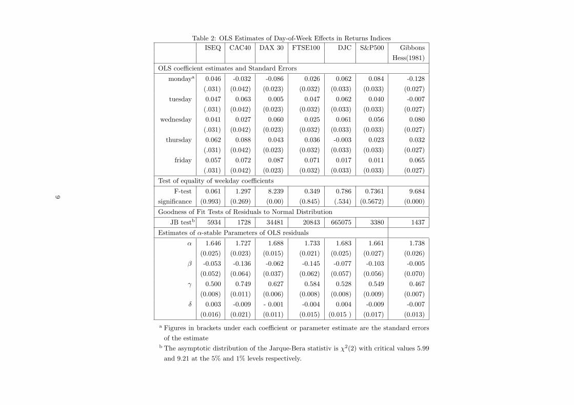
Table 2: OLS Estimates of Day-of-Week Effects in Returns Indices

ISEQ CAC40 DAX 30 FTSE100 DJC S&P500 Gibbons

Hess(1981)

OLS coefficient estimates and Standard Errors

mondaya 0.046 -0.032 -0.086 0.026 0.062 0.084 -0.128

(.031) (0.042) (0.023) (0.032) (0.033) (0.033) (0.027)

tuesday 0.047 0.063 0.005 0.047 0.062 0.040 -0.007

(.031) (0.042) (0.023) (0.032) (0.033) (0.033) (0.027)

wednesday 0.041 0.027 0.060 0.025 0.061 0.056 0.080

(.031) (0.042) (0.023) (0.032) (0.033) (0.033) (0.027)

thursday 0.062 0.088 0.043 0.036 -0.003 0.023 0.032

(.031) (0.042) (0.023) (0.032) (0.033) (0.033) (0.027)

friday 0.057 0.072 0.087 0.071 0.017 0.011 0.065

(.031) (0.042) (0.023) (0.032) (0.033) (0.033) (0.027)

Test of equality of weekday coefficients

F-test 0.061 1.297 8.239 0.349 0.786 0.7361 9.684

significance (0.993) (0.269) (0.00) (0.845) (.534) (0.5672) (0.000)

Goodness of Fit Tests of Residuals to Normal Distribution

JB testb 5934 1728 34481 20843 665075 3380 1437

Estimates of α-stable Parameters of OLS residuals

α 1.646 1.727 1.688 1.733 1.683 1.661 1.738

(0.025) (0.023) (0.015) (0.021) (0.025) (0.027) (0.026)

β -0.053 -0.136 -0.062 -0.145 -0.077 -0.103 -0.005

(0.052) (0.064) (0.037) (0.062) (0.057) (0.056) (0.070)

γ 0.500 0.749 0.627 0.584 0.528 0.549 0.467

(0.008) (0.011) (0.006) (0.008) (0.008) (0.009) (0.007)

δ 0.003 -0.009 - 0.001 -0.004 0.004 -0.009 -0.007

(0.016) (0.021) (0.011) (0.015) (0.015 ) (0.017) (0.013)

a Figures in brackets under each coefficient or parameter estimate are the standard errors

of the estimateb The asymptotic distribution of the Jarque-Bera statistiv is χ2(2) with critical values 5.99

and 9.21 at the 5% and 1% levels respectively.

9

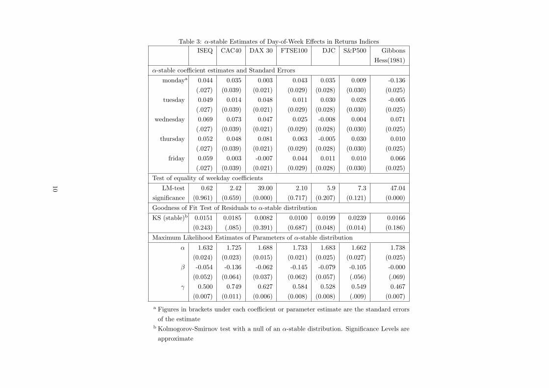
Table 3: α-stable Estimates of Day-of-Week Effects in Returns Indices

ISEQ CAC40 DAX 30 FTSE100 DJC S&P500 Gibbons

Hess(1981)

α-stable coefficient estimates and Standard Errors

mondaya 0.044 0.035 0.003 0.043 0.035 0.009 -0.136

(.027) (0.039) (0.021) (0.029) (0.028) (0.030) (0.025)

tuesday 0.049 0.014 0.048 0.011 0.030 0.028 -0.005

(.027) (0.039) (0.021) (0.029) (0.028) (0.030) (0.025)

wednesday 0.069 0.073 0.047 0.025 -0.008 0.004 0.071

(.027) (0.039) (0.021) (0.029) (0.028) (0.030) (0.025)

thursday 0.052 0.048 0.081 0.063 -0.005 0.030 0.010

(.027) (0.039) (0.021) (0.029) (0.028) (0.030) (0.025)

friday 0.059 0.003 -0.007 0.044 0.011 0.010 0.066

(.027) (0.039) (0.021) (0.029) (0.028) (0.030) (0.025)

Test of equality of weekday coefficients

LM-test 0.62 2.42 39.00 2.10 5.9 7.3 47.04

significance (0.961) (0.659) (0.000) (0.717) (0.207) (0.121) (0.000)

Goodness of Fit Test of Residuals to α-stable distribution

KS (stable)b 0.0151 0.0185 0.0082 0.0100 0.0199 0.0239 0.0166

(0.243) (.085) (0.391) (0.687) (0.048) (0.014) (0.186)

Maximum Likelihood Estimates of Parameters of α-stable distribution

α 1.632 1.725 1.688 1.733 1.683 1.662 1.738

(0.024) (0.023) (0.015) (0.021) (0.025) (0.027) (0.025)

β -0.054 -0.136 -0.062 -0.145 -0.079 -0.105 -0.000

(0.052) (0.064) (0.037) (0.062) (0.057) (.056) (.069)

γ 0.500 0.749 0.627 0.584 0.528 0.549 0.467

(0.007) (0.011) (0.006) (0.008) (0.008) (.009) (0.007)

a Figures in brackets under each coefficient or parameter estimate are the standard errors

of the estimateb Kolmogorov-Smirnov test with a null of an α-stable distribution. Significance Levels are

approximate

10

Table 4: Summary Statistics DAX30 Total Returns and fit to Normal and

α-Stable Distributions for three sub periods

start date 29/09/59 28/01/75 29/05/90

end date 27/01/75 28/05/90 26/09/05

observations 4000 4000 4000

mean 0.004 0.036 0.025

St. dev 0.989 0.978 1.424

Skewness 0.518 -1.061 -0.276

Kurtosis 8.633 17.940 4.110

Goodness of Fit Tests for Normal Distribution

JB testa 1287 54389 2874.23

KS testb 0.044 0.058 0.072

SW testc 0.952 0.907 0.949

Estimates of of α-stable Parameters of Return Distribution

αd 1.820 1.777 1.636

(0.022) (0.023) (0.027)

β 0.059 -0.066 -0.168

(0.095) (0.082) (0.056)

γ 0.601 0.553 0.774

(0.009) (0.008) (0.013)

δ 0.001 0.040 0.008

Goodness of Fit Tests for α-Stable Distribution

KS (stable) 0.012 0.012 0.023

p-value 0.619 0.652 0.034

a The asymptotic distribution of the Jarque-Bera statistiv is χ2(2) with

critical values 5.99 and 9.21 at the 5% and 1% levels respectively.b For the sample sizes here the 1% critical value for the Kolmogorov-Smirnov

statistic is less that .02. See Marsaglia et al. (2003)c The 5% critical level for the Shapiro Wilk test is .9992 for a sample of 4500.

The smaller values reported here indicate very significant departures from

normality.d Figures in brackets under each coefficient estimate are asymptotic stan-

dard errors

11

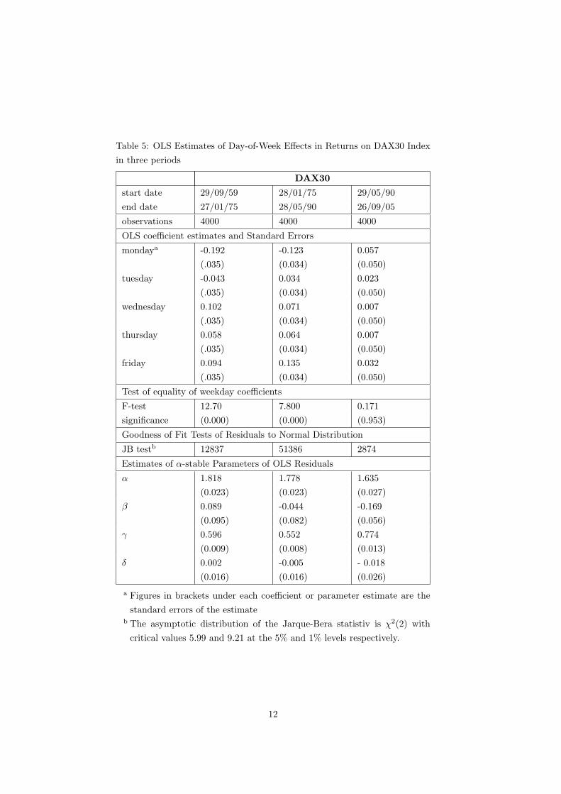
Table 5: OLS Estimates of Day-of-Week Effects in Returns on DAX30 Index

in three periods

DAX30

start date 29/09/59 28/01/75 29/05/90

end date 27/01/75 28/05/90 26/09/05

observations 4000 4000 4000

OLS coefficient estimates and Standard Errors

mondaya -0.192 -0.123 0.057

(.035) (0.034) (0.050)

tuesday -0.043 0.034 0.023

(.035) (0.034) (0.050)

wednesday 0.102 0.071 0.007

(.035) (0.034) (0.050)

thursday 0.058 0.064 0.007

(.035) (0.034) (0.050)

friday 0.094 0.135 0.032

(.035) (0.034) (0.050)

Test of equality of weekday coefficients

F-test 12.70 7.800 0.171

significance (0.000) (0.000) (0.953)

Goodness of Fit Tests of Residuals to Normal Distribution

JB testb 12837 51386 2874

Estimates of α-stable Parameters of OLS Residuals

α 1.818 1.778 1.635

(0.023) (0.023) (0.027)

β 0.089 -0.044 -0.169

(0.095) (0.082) (0.056)

γ 0.596 0.552 0.774

(0.009) (0.008) (0.013)

δ 0.002 -0.005 - 0.018

(0.016) (0.016) (0.026)

a Figures in brackets under each coefficient or parameter estimate are the

standard errors of the estimateb The asymptotic distribution of the Jarque-Bera statistiv is χ2(2) with

critical values 5.99 and 9.21 at the 5% and 1% levels respectively.

12

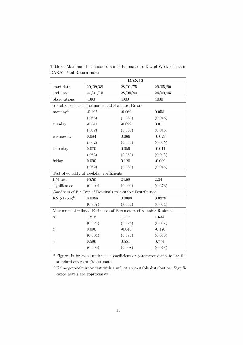
Table 6: Maximum Likelihood α-stable Estimates of Day-of-Week Effects in

DAX30 Total Return Index

DAX30

start date 29/09/59 28/01/75 29/05/90

end date 27/01/75 28/05/90 26/09/05

observations 4000 4000 4000

α-stable coefficient estimates and Standard Errors

mondaya -0.195 -0.069 0.058

(.033) (0.030) (0.046)

tuesday -0.041 -0.029 0.011

(.032) (0.030) (0.045)

wednesday 0.084 0.066 -0.029

(.032) (0.030) (0.045)

thursday 0.070 0.059 -0.011

(.032) (0.030) (0.045)

friday 0.090 0.120 -0.009

(.032) (0.030) (0.045)

Test of equality of weekday coefficients

LM-test 60.50 23.08 2.34

significance (0.000) (0.000) (0.673)

Goodness of Fit Test of Residuals to α-stable Distribution

KS (stable)b 0.0098 0.0098 0.0279

(0.837) (.0836) (0.004)

Maximum Likelihood Estimates of Parameters of α-stable Residuals

α 1.818 1.777 1.634

(0.023) (0.024) (0.027)

β 0.090 -0.048 -0.170

(0.094) (0.082) (0.056)

γ 0.596 0.551 0.774

(0.009) (0.008) (0.013)

a Figures in brackets under each coefficient or parameter estimate are the

standard errors of the estimateb Kolmogorov-Smirnov test with a null of an α-stable distribution. Signifi-

cance Levels are approximate

13

The final column in each table gives results corresponding to those in Gibbons and Hess

(1981). Although I use a different equity index my results are very similar. The Monday

effect is negative and very significant in both cases and the OLS and α-stable estimates

are very similar. Thus the Gibbons and Hess (1981) results are robust with respect to

the specification of residals.

This “Monday effect” effect found in the Gibbons and Hess (1981) sample period is not

significant in the five total returns indices (ISEQ, CAC40, FTSE100, DJC and S&P500).

This corresponds to recent analysis which has found that the “Monday effect” has been

becoming smaller and even positive in recent times (see for example Hansen et al. (2005)).

It should be noted that although there are some differences in the return patterns when

comparing the OLS and Maximum Likelihood α-stable estimates it is not obvious how

any statistical significance could be attached to this result. Specific weekday effects such

as the “Monday effect” have often been justified only after a significant weekday effect

has been found. In an experimental science this could be verified by further independent

experimental studies. In economics we rarely have this facility. Sullivan et al. (2001)

lists a large number of possible seasonal effects. Some of these are likely to occur by

chance and will then be found by a specification search. The danger of data-mining is

very real.

The longer return series for the DAX30 shows a significant day of the week effect in both

OLS and α-stable cases. The OLS analysis points to significantly low returns on Monday

and high returns on Friday as the cause of the problem. The α-stable results point to

significantly higher returns on Thursday. The contradiction in this result highlights the

danger of data mining in this case. The point has been discussed at length in Sullivan

et al. (2001).

Table 4 gives summary statistics of returns on the DAX30 for three periods, 29 Septem-

ber 1959 to 27 January 1975, 28 January 1975 to 28 May 1990 and 29 May 1990 to 27

September 2005. The normal distribution is a poor fit to the data. The α-stable distrib-

ution provides a good fit for the first two periods. The goodness of fit test for an α-stable

distribution fails for the third period The p-values in are based on the assumption of

known parameters and thus possible underestimate the fit.

Tables (5) and (3) set out OLS and α-stable maximum likelihood estimates of the day

of week effects in each or these subperiods. The results are very similar in both sets of

tests. In the first two periods the hypothesis of no weekday effect is rejected and in the

third period the hypothesis can not be rejected in both the OLS and α-stable analysis.

In the α-stable analysis for the two early periods the Thursday return is significantly

higher than the average. This is not so in the OLS analysis.

It should be noted that the stability parameter in the fit of all residuals to an α-stable

distribution is significantly less than 2 indicating deficiencies in the assumption of a

normal distribution.

14

4 Summary and Conclusions

This paper sets out the theory of maximum likelihood estimation and of a linear re-

gression when residuals follow an α-stable distribution. This theory is then applied to

the estimation and testing for a “weekday effects” in returns on equity indices. I have

found that maximum likelihood estimation of a linear regression with α-stable residuals

is feasible.

Traditional OLS estimation and testing is carried out in parallel and the results are

compared. Of the ten regressions completed significant “weekday effects” effects were

found in the same four in both the α-stable and OLS systems. However the alternative

methodologies attributed significance to different daily effects. The α-stable distribution

appeared to be a better fit to the residuals in both OLS and α-stable estimates and on

the basis of specification the α-stable estimation is to be preferred.

“weekday effects” such as the “Monday effect”, found in some of the regressions here,

are often justified by theories relating to institutional arrangements. A “Monday effect”

has been explained by delays in trading and settlement caused by the weekend. Such

explanations are often given after the significant result has been found leading to ac-

cusations of data mining. As I did not have a prior theory explaining the extra effects

found in the α-stable estimates any conclusions that I might draw would, justifiably, be

subject to the same criticisms. The conclusion remains that if individual coefficients are

of interest, the residuals have fat tails and a possible α-stable distribution the results

should be checked for robustness using methods such as those employed here.

15

References

Adler, R. J., R. E. Feldman, and M. S. Taqqu (Eds.) (1998). A Practical Guide to Heavy

Tails: Statistical Techniques and Applications. Birkhauser.

Bachelier, L. (1900). Theorie de la Speculation, theorie mathematique du jeu. Ph. D.

thesis, Ecole Normale Sup.

Cootner, P. H. (Ed.) (1964). The Random Character of Stock Market Prices. M.I.T.

Press. Reprinted 2000 by Risk Publications.

DuMouchel, W. H. (1971). Stable Distributions in Statistical Inference. Ph. D. thesis,

Yale University.

DuMouchel, W. H. (1973, September). On the asymptotic normality of the maximum

likelihood estimate when sampling from a stable distribution. The Annals of Statis-

tics 1 (5), 948–957.

DuMouchel, W. H. (1975, June). Stable Distributions in Statistical Inference: 2. Infer-

ence from Stably Distributed Samples. Ph. D. thesis.

Fama, E. F. and R. Roll (1968, September). Some properties of symmetric stable dis-

tributions. Journal of the American Statistical Association 63 (323), 817–836.

Feller, W. (1966). An Introduction to Probability Theory and its Applications, Volume

II. Wiley.

Gibbons, M. R. and P. Hess (1981). Day of the week effects and asset returns. The

Journal of Business 54, 579–596.

Gut, A. (2005). Probability: A Graduate Course. Springer.

Hansen, P. R., A. Lunde, and J. M. Nason (2005, January). Testing the significance of

calendar effects. Working Paper 2005-2, Federal Reserve Bank of Atlanta.

Janicki, A. and A. Weron (1994). Simulation and ChaoticBehavior of α-Stable Stochastic

Processes. Dekker.

Logan, B. F., C. L. Mallows, S. Rice, and L. A. Shepp (1973, October). Limit distribu-

tions of self-normalized sums. The Annals of Probability 1 (5), 788–809.

Mandelbrot, B. B. (1962, March). The variation of certain speculative prices. Technical

Report NC-87, IBM Research Report.

Mandelbrot, B. B. (1964). The Variation of Certain Speculative Prices, Chapter 15,

Cootner (1964), pp. 307–332. M.I.T. Press.

Mandelbrot, B. B. (1967). The variation of the prices of cotton, wheat, and railroad

stocks, and of some financial rates. The Journal of Business 40, 393–413.

16

Mandelbrot, B. B. and R. L. Hudson (2004). The (mis)Behaviour of Markets. Profile

Books.

Marsaglia, G., W. W. Tsang, and J. Wang (2003). Evaluating Kolmogorov’s distribution.

Journal of Statistical Software 8/18.

McCulloch, J. H. (1998). Linear regression with stable distributions. In Adler et al.

(1998).

Nolan, J. P. (2005, Feb.). STABLE program. Available for download from http:

//academic2.american.edu/∼jpnolan/stable/stable.exel.

Nolan, J. P. (2006). Stable distributions - models for heavy tailed data. Birkhauser, In

progress Chapter 1 available online at academic2/american.edu/∼jpnolan.

Pettengill, G. N. (2003). A survey of the monday effect literature. Quarterly Journal of

Business and Economics 42 (3/4), 3–27.

R Development Core Team (2006). R: A Language and Environment for Statistical

Computing. Vienna, Austria: R Foundation for Statistical Computing. ISBN 3-

900051-07-0.

Rachev, S. and S. Mittnik (2000). Stable Paretian Models in Finance. Wiley.

Rimmer, R. H. (2005). Calculation of stable distributions with mathematica.

http://www.npgcable.com/ rrimmer/StableCalculation/.

Samorodnitsky, G. and M. S. Taqqu (1994). Stable Non-Gaussian Random Processes

Stochastic Models with Infinite Variance. Chapman and Hall/CRC.

Sullivan, R., A. Timmermann, and H. White (2001). Dangers of data mining: The case

of calendar effects in stock returns. Journal of Econometrics 105, 249–286.

Uchaikin, V. V. and V. M. Zolotarev (1999). Chance and Stability. VSP, Uthrecht.

Weron, R. (1998). Modelling Volatility of Financial Time Series. Ph. D. thesis, The

Hugo Steinhaus Center, Wroc?aw University of Technology.

Wolfram, S. (2003). The Mathematica Book (5th ed.). Wolfram Media.

Wuertz, D. (2005). Rmetrics - an environment for teaching financial engineering and

computational finance with R. Institute for Theoretical Physics, Swiss Federal Insti-

tute of Technology, Zurich.

Zolotarev, V. M. (1986). One-dimensional Stable Distributions. Translations of Mathe-

matical Monographs, Volume 65, American Mathematical Society.

17

A An Introduction to α-Stable Processes

Some limit properties of normal random variables

This section outlines the properties of the α-stable family of distributions and compares

those with the standard normal distribution. Proofs are not given. These and further

details may be found in Feller (1966), Janicki and Weron (1994), Rachev and Mittnik

(2000), Samorodnitsky and Taqqu (1994), Uchaikin and Zolotarev (1999) or Zolotarev

(1986).

An assumption of a normal distribution has formed part of almost all developments in

theoretical and empirical finance in the last half century. In the introduction we have

already referred to the Capital Asset Pricing Model, optimal portfolio allocation and

option pricing as depending on a normality assumption. Some form of central3 limit

theorem has been implicit in all these developments. The theorem as quoted in many

econometric tests may be weakened. A version in Gut (2005) is as follows

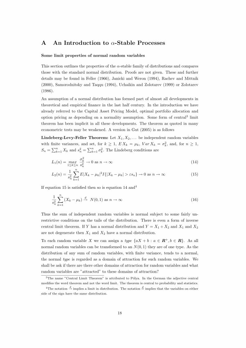
Lindeberg-Levy-Feller Theorem: Let X1,X2, . . . be independent random variables

with finite variances, and set, for k ≥ 1, E Xk = µk, V ar Xk = σ2k, and, for n ≥ 1,

Sn =∑n

k=1 Xk and s2n =

∑nk=1 σ2

k. The Lindeberg conditions are

L1(n) = max1≤k≤n

σ2k

s2n

→ 0 as n → ∞ (14)

L2(n) =1

s2n

n∑

k=1

E|Xk − µk|2I{|Xk − µk| > εsn} → 0 as n → ∞ (15)

If equation 15 is satisfied then so is equation 14 and4

1

s2n

n∑

k=1

(Xk − µk)d→ N(0, 1) as n → ∞ (16)

Thus the sum of independent random variables is normal subject to some fairly un-

restrictive conditions on the tails of the distribution. There is even a form of inverse

central limit theorem. If Y has a normal distribution and Y = X1 + X2 and X1 and X2

are not degenerate then X1 and X2 have a normal distribution.

To each random variable X we can assign a type {aX + b : a ∈ R+, b ∈ R}. As all

normal random variables can be transformed to an N(0, 1) they are of one type. As the

distribution of any sum of random variables, with finite variance, tends to a normal,

the normal type is regarded as a domain of attraction for such random variables. We

shall be ask if there are there other domains of attraction for random variables and what

random variables are ”attracted” to these domains of attraction?

3The name ”Central Limit Theorem” is attributed to Polya. In the German the adjective central

modifies the word theorem and not the word limit. The theorem is central to probability and statistics.

4The notationd→ implies a limit in distribution. The notation

d= implies that the variables on either

side of the sign have the same distribution.

18

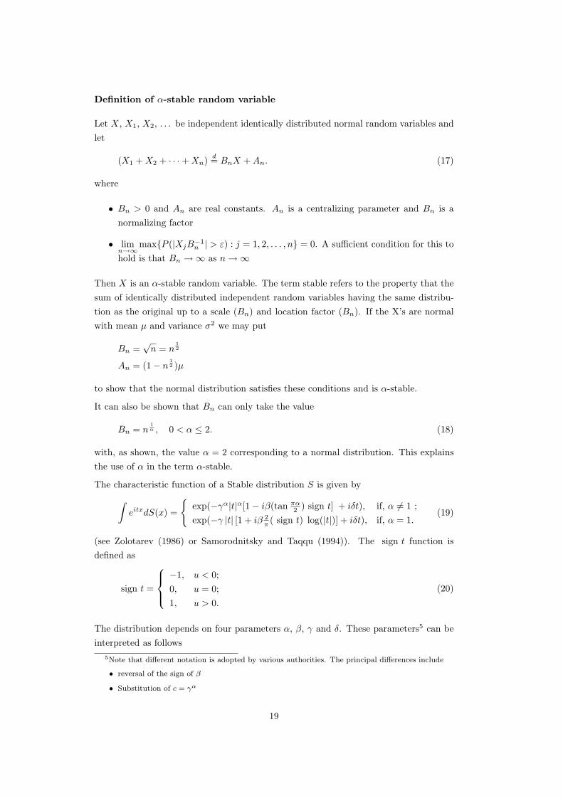
Definition of α-stable random variable

Let X, X1, X2, . . . be independent identically distributed normal random variables and

let

(X1 + X2 + · · · + Xn)d= BnX + An. (17)

where

• Bn > 0 and An are real constants. An is a centralizing parameter and Bn is a

normalizing factor

• limn→∞

max{P (|XjB−1n | > ε) : j = 1, 2, . . . , n} = 0. A sufficient condition for this to

hold is that Bn → ∞ as n → ∞

Then X is an α-stable random variable. The term stable refers to the property that the

sum of identically distributed independent random variables having the same distribu-

tion as the original up to a scale (Bn) and location factor (Bn). If the X’s are normal

with mean µ and variance σ2 we may put

Bn =√

n = n1

2

An = (1 − n1

2 )µ

to show that the normal distribution satisfies these conditions and is α-stable.

It can also be shown that Bn can only take the value

Bn = n1

α , 0 < α ≤ 2. (18)

with, as shown, the value α = 2 corresponding to a normal distribution. This explains

the use of α in the term α-stable.

The characteristic function of a Stable distribution S is given by

∫

eitxdS(x) =

{

exp(−γα|t|α[1 − iβ(tan πα2 ) sign t] + iδt), if, α 6= 1 ;

exp(−γ |t| [1 + iβ 2π ( sign t) log(|t|)] + iδt), if, α = 1.

(19)

(see Zolotarev (1986) or Samorodnitsky and Taqqu (1994)). The sign t function is

defined as

sign t =

−1, u < 0;

0, u = 0;

1, u > 0.

(20)

The distribution depends on four parameters α, β, γ and δ. These parameters5 can be

interpreted as follows

5Note that different notation is adopted by various authorities. The principal differences include

• reversal of the sign of β

• Substitution of c = γα

19

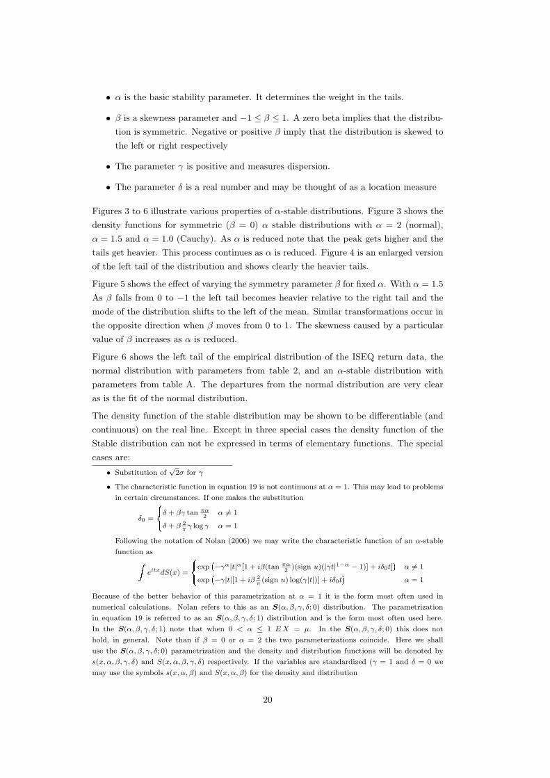
• α is the basic stability parameter. It determines the weight in the tails.

• β is a skewness parameter and −1 ≤ β ≤ 1. A zero beta implies that the distribu-

tion is symmetric. Negative or positive β imply that the distribution is skewed to

the left or right respectively

• The parameter γ is positive and measures dispersion.

• The parameter δ is a real number and may be thought of as a location measure

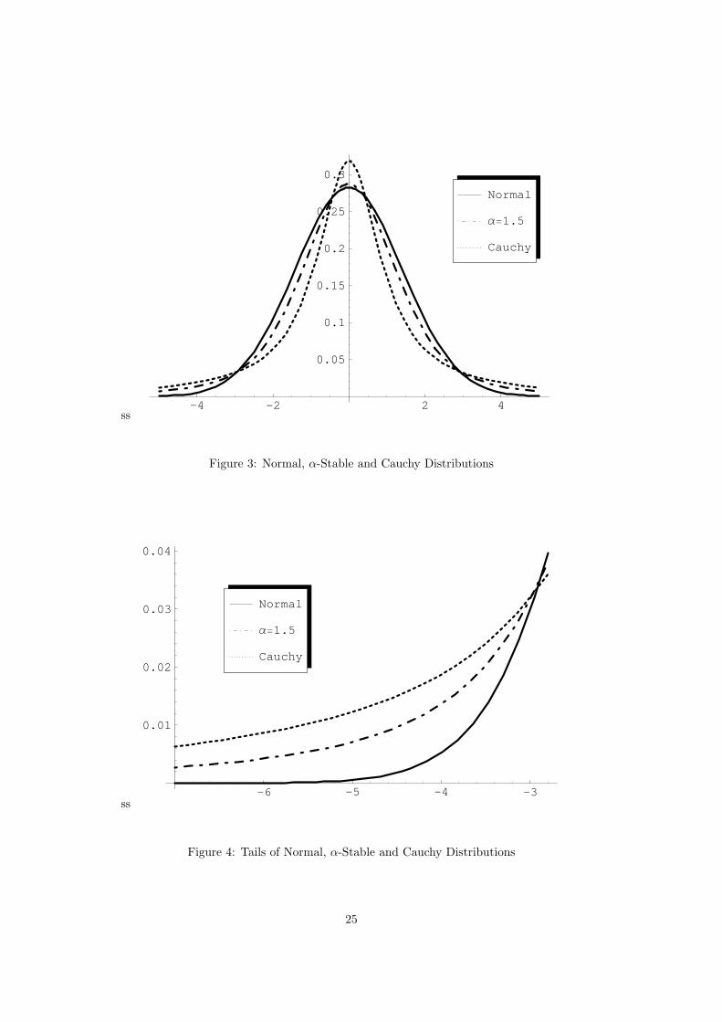
Figures 3 to 6 illustrate various properties of α-stable distributions. Figure 3 shows the

density functions for symmetric (β = 0) α stable distributions with α = 2 (normal),

α = 1.5 and α = 1.0 (Cauchy). As α is reduced note that the peak gets higher and the

tails get heavier. This process continues as α is reduced. Figure 4 is an enlarged version

of the left tail of the distribution and shows clearly the heavier tails.

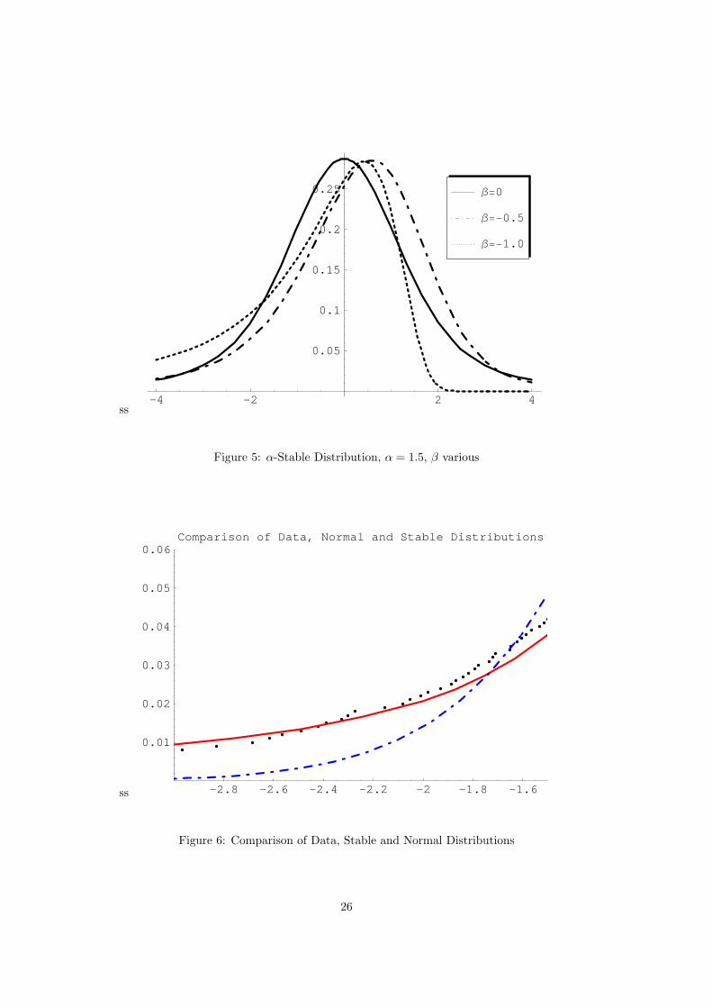
Figure 5 shows the effect of varying the symmetry parameter β for fixed α. With α = 1.5

As β falls from 0 to −1 the left tail becomes heavier relative to the right tail and the

mode of the distribution shifts to the left of the mean. Similar transformations occur in

the opposite direction when β moves from 0 to 1. The skewness caused by a particular

value of β increases as α is reduced.

Figure 6 shows the left tail of the empirical distribution of the ISEQ return data, the

normal distribution with parameters from table 2, and an α-stable distribution with

parameters from table A. The departures from the normal distribution are very clear

as is the fit of the normal distribution.

The density function of the stable distribution may be shown to be differentiable (and

continuous) on the real line. Except in three special cases the density function of the

Stable distribution can not be expressed in terms of elementary functions. The special

cases are:

• Substitution of√

2σ for γ

• The characteristic function in equation 19 is not continuous at α = 1. This may lead to problems

in certain circumstances. If one makes the substitution

δ0 =

8<:δ + βγ tan πα

2α 6= 1

δ + β 2π

γ log γ α = 1

Following the notation of Nolan (2006) we may write the characteristic function of an α-stable

function asZeitxdS(x) =

8<:exp�−γα|t|α[1 + iβ(tan πα

2)(sign u)(|γt|1−α − 1)] + iδ0t]

�α 6= 1

exp�−γ|t|[1 + iβ 2

π(sign u) log(γ|t|)] + iδ0t

�α = 1

Because of the better behavior of this parametrization at α = 1 it is the form most often used in

numerical calculations. Nolan refers to this as an S(α, β, γ, δ; 0) distribution. The parametrization

in equation 19 is referred to as an S(α, β, γ, δ; 1) distribution and is the form most often used here.

In the S(α, β, γ, δ; 1) note that when 0 < α ≤ 1 E X = µ. In the S(α, β, γ, δ; 0) this does not

hold, in general. Note than if β = 0 or α = 2 the two parameterizations coincide. Here we shall

use the S(α, β, γ, δ; 0) parametrization and the density and distribution functions will be denoted by

s(x, α, β, γ, δ) and S(x, α, β, γ, δ) respectively. If the variables are standardized (γ = 1 and δ = 0 we

may use the symbols s(x, α, β) and S(x, α, β) for the density and distribution

20

Normal Description If α = 2 the characteristic function in equation (19) reduces to

φ(it) =

∫

eitxdH(x) = exp(iδt + γ2t2) (21)

Which is the characteristic function of a normal distribution

1

γ√

πexp

(x − δ)2

γ2, −∞ < x < ∞

with mean δ and variance 2γ2. Note that the symmetry parameter does not appear

in the characteristic function in this case.

Cauchy Distribution When α = 1 and β = 0 the characteristic function reduces to

exp(−γ|t| + iδt)

which is the characteristic function of the Cauchy Distribution

1

π(γ2 + (x − δ)2), −∞ < x < ∞

Levy Distribution When α = 1/2 and β = −1 the distribution becomes a Levy

distribution( σ

2π

)1/2 1

(x − µ)3/2exp

(

− σ

2(x − µ)

)

, µ < x < ∞

Generalized Central Limit Theorem – Domains of attraction

Consider a random variable X with density function such that

F (x) ∼

B−|x|−(1+a) as x → −∞B+|x|−(1+a) as x → ∞

(22)

where 0 < a < 2. Thus the tails of the distribution have an asymptotic Pareto6 distrib-

ution. Put

b =B+ − B−

B+ + B−

(23)

6The Pareto distribution was used by Pareto almost on hundred years ago to model the distribution

of incomes above a certain threshold. A random variable has a Pareto distribution if its density function

is of the form:

fX(x; a, b) = abax−(1+a) x > b, a > 0, b > 0

This distribution has a remarkable property known as scaling. If we increase the threshold the shape

of the distribution remains the same apart from a scaling factor. For example, by integration, P [X ≥cb] = c−a. Then the distribution of X given that X ≥ cb, where c > 1 is given by

fX(x; a, cb) = a(cb)ax−(1+a) x > cb, a > 0, b > 0, c > 1

Thus P [X ≥ c2b|X ≥ 2b] = c−a. To illustrate let the distribution of the wealth of persons with wealth

greater than say e1, 000, 000 be Pareto with parameter a = 1.5 Then the probability that a person in

this group will have wealth of twice the threshold is about 0.35. Now let the threshold be e2, 000, 000

then the probability that a person above that threshold will have a wealth of twice that threshold

(e4, 000, 000) is again 0.35. This is in complete contrast to the normal or lognormal distribution. Note

that the mean of this distribution exists if a > 1 and the variance if a > 2.

21

Then if X1, X3, . . . Xn are independent, identically distributed random variables with

this asymptotic distribution then the random variable

S =1

n1

a

n∑

i=1

Xi (24)

has a limit in distribution which is α-stable with parameters α = a and β = b

Thus each member of the family of α-stable distributions possesses a domain of attrac-

tion. This domain includes all distributions with the Pareto tails described in equa-

tion 22.

Some properties of α-stable distributions

Some of the more important properties of α-stable distributions ar given below

• The only α-stable distribution for which moments of all orders exist is the normal

distribution. When 1 < α < 2 the variance is not defined (infinite) and only the

mean exists. In our notation the mean is given by EX = δ. Apart from the lack

of a simple form for the density function of an α-stable density function the non-

existence of a variance is the greatest barrier to their use. Put simply measures

of the variance of an α-stable process will increase with sample size and will not

converge.

If 0 < α ≤ 1 the mean does not exist. If α < 1 the mean is even more dispersed

than the individual measurements. In applications of α-stable distributions to

finance values of α are usually of the order of 1.5 to 1.8 are usually appropriate.

The values estimated in section 3 vary from 1.63 to 1.73.

• The α-stable density is symmetric with respect to simultaneous changes of the sign

of x and β, that is

s(x, α, β, γ, δ) = s(−x,−β, γ, δ) (25)

• If a and b > 0 are real constants then the density of x−ab is given by

1

bs(

x − a

b, α, β,

γ

b,δ − a

b) (26)

or in particular that of x−δγ by

1

γs(

x − δ

γ, α, β, 1, 0) (27)

where s(x, α, β, γ, δ) is the density of x. δ and γ are described as location and

scale parameters respectively.

• Let X1 and X2 be α-stable random variables with densities s(x, α, βi, γi, δi), i =

1, 2. Then X1 + X2 is α-stable with

β =β1γ

α1 + β2γ

α2

γα1 + γα

2

, γ = (γα1 + γα

2 )1

α , δ = δ1 + δ2 (28)

22

In general use, the density functions of an α-stable process may be estimated by an

inverse numerical transform of the characteristic function. For some purposes the nu-

merical integration routines in Mathematica (Wolfram (2003)) may be sufficient. To

provide greater accuracy in the tails of the distribution some form of series or integral

expansion of the characteristic function is often used. Programs to compute α-stable

density and distribution functions are available in Mathematica (Rimmer (2005)), R

(Wuertz (2005)) or as the stand-alone program STABLE (Nolan (2005)). The calcula-

tions in this paper make considerable use of these packages.

23

-6 -4 -2 2 4 6

0.25

0.5

0.75

1

1.25

1.5

Normal

Α = 1.6

Α = 1.2

Figure 1: Comparison of implied weights in GLS equivalent of Maximum Likelihood

estimates of regression coefficient when residuals are distributed as symmetric α stable

variates

-6 -4 -2 2 4 6

-1

1

2

Normal

Α = 1.6

Α = 1.2

Figure 2: Comparison of implied weights in GLS equivalent of Maximum Likelihood

estimates of regression coefficient when residuals are distributed as skewed α stable

variables with β = −0.1

24

ss-4 -2 2 4

0.05

0.1

0.15

0.2

0.25

0.3

Cauchy

Α=1.5

Normal

Figure 3: Normal, α-Stable and Cauchy Distributions

ss-6 -5 -4 -3

0.01

0.02

0.03

0.04

Cauchy

Α=1.5

Normal

Figure 4: Tails of Normal, α-Stable and Cauchy Distributions

25

ss-4 -2 2 4

0.05

0.1

0.15

0.2

0.25

Β=-1.0

Β=-0.5

Β=0

Figure 5: α-Stable Distribution, α = 1.5, β various

ss -2.8 -2.6 -2.4 -2.2 -2 -1.8 -1.6

0.01

0.02

0.03

0.04

0.05

0.06Comparison of Data, Normal and Stable Distributions

Figure 6: Comparison of Data, Stable and Normal Distributions

26