Maximum Likelihood Estimators in a Statistical Model of

Maximum Likelihood Estimators in a Statistical Model of Natural Catastrophe Claims with Trend

ALEXANDER KUKUSH Kiev National Taras Shevchenko University, Volodymyrska 60, 01033 Kiev, Ukraine E-mail: [email protected]

YURI CHERNIKOV Celenia Software, Rybalska 22, 01011 Kiev, Ukraine E-mail: [email protected]

DIETMAR PFEIFER University Oldenberg, Fachbereich Mathematik, P.O. Box 2503, D-26111 Oldenburg, Germany E-mail: pfeifer@mathematik.!lni-oldenburg.de

Abstract. A statistical model to analyse stochastically increasing claims arising out of natural catastrophes is presented. Based on record values, the exponential trends over time can be identified. A more specific threeparameter model involving such a trend is also proposed. Observed claims are modeled as a stochastically increasing sequence of Frechet distributed random variables. Consistency and asymptotic normality of the joint maximum likelihood estimator are shown. Possible applications in forecasting of claims are indicated. In particular claims data from U.S. hurricanes and Japanese taifuns are discussed.

Key words. catastrophe claims, Frechet distribution, maximum likelihood estimator, Nevzorov's record model, trend

AMS 2000 subject classifications.

1. Introduction

Primary-62P05. 62F 12.

Secondary-62H 12

It is evident that insurance claims due to the occurrence of natural catastrophes have raised enormously over the past decades all over the world, in particular w.r.t. wind storm losses. We present a particular approach to the investigation of catastrophe claims in the presence of a trend, which is based on a combinations of parametric and semiparametric methods. In the first step, the type of trend is analyzed using the number of record values in the times series of claims data, and in the second step, a maximumlikelihood estimator (MLE) is constructed from the data taking into account what type of trend has been detected before. In order to check the validity of the model assumptions, the estimates for the trend parameter obtained from both steps can be compared.

1

The proposed combination of semi-parametric and parametric models is due to Pfeifer (1997). In the present paper the asymptotic properties of the estimators are presented. They are important in forecasting of claims.

In some articles issued during last time there were some attempts to investigate this area. However no author succeeded in proving consistency in non-i.i.d case. Thus in Smith and Goodman (2000) insurance data claims obtained from a large company are analyzed to determine the distribution of tail values. The effect of possible trends in the observed data is considered. In McNeil and Saladin (2000) the peaks-over-threshold method is used to derive a natural model for the point process oflarge losses exceeding a high threshold. This model is used to obtain a joint description of the frequency and the severity with which large losses occur. In Coles (2001) the model diagnostics for a nonhomogeneous in time model is considered. In Rootzen and Tajvidi (1997) the statistical extreme value theory is reviewed and some examples are given which show how to use it in large claims insurance.

A weaker version of the asymptotic results was announced in Kukush (1999). We mention that a goodness-of-fit test for both semi-parametric and three-parametric models was constructed in Kukush and Chemikov (2001), and in Kukush and Chemikov (2002) it is shown that in both models the MLE are asymptotically efficient in the sense of Hajek bound.

The present paper is organized as follows. In Section 2 Nevzorov's record model is introduced. In Section 3 the consistency and asymptotic normality results of the semiparametric MLE are formulated. Section 4 contains the three-parametric model and the corresponding consistency and asymptotic normality results. In Section 5 the semiparametric and the three-parametric approaches in data analysis are compared, Section 6 contains simulations. Implications for insurance applications are considered in Section 7, Section 8 concludes, and the proofs are given is Section 9.

2. Nevzorov's record model

A record model has been studied by Nevzorov (1988) and Borovkov and Pfeifer (1995). Assume that the yearly catastrophe claims considered here are realizations of an independent sequence {Xm n ;::: I} of random variables (r.v.) with support R+ := [0, 00) and continuous cumulative d.f. {Fm n ;::: I}, s.t.

Fn = F'rn, with 'Yn := 'Yn- I , 'Y ;::: 1.

Here F is a fixed cumulative d.f. with F(O) = O. Define record indicators by

{I, if Xn > max{XI"" ,Xn- d

II := 1, In:= 0, otherwise for n ;::: 2,

(2.1 )

2

i.e., In = 1 iff observation Xn is a record value in the sequence. Under the above assumptions, the record indicators are independent r.v. with

Pn(-y) :=P"!(In = 1) =,1 +!~ +,n = 1 +, 1+1 ... +, n+l·

Consider also the number Sn of record values in a finite number of observations,

n

Sn := LI;, n:::: 1. ;=1

The record times TI , . •. TSn denote the observation times at which record values occur:

TI := 1, Tk+1 := min {i:::; niX; > X Tk }, 1 :::; k < Sn.

The unknown parameter " see (2.1), is called trend parameter. If, = 1, then we have the i.i.d. situation (no trend), while for, > 1, the r.v. {Xn} are stochastically increasing (positive trend). Given the observations I" ... , 1m n :::: 2, of record indicators in a sequence of data, the log-likelihood function L(r) for, :::: 1 is given by

L(-y) = In (gP;(-y)t;(l - p;(-y))I-t)

n n

= LI; In(p;(-y)) + L (1 - I;) In (1 - p;(-y)). (2.2) ;=2 ;=2

For, > 1 it is possible to rewrite it in a way, which is more comfortable for numerical optimization:

s" L(-y) = Sn In (-y - 1) - In (-yn - 1) - L In (1 - ,I -Tk) • (2.3)

k=2

The semi-parametric MLE i = in is defined as a measurable function of h, . .. , 1m for which

i E arg max L(-y). ,,!:O::1

(2.4)

If I" ... , In i= (1, 1, ... , 1), then maximum in (2.4) is attained. Otherwise the maximum in (2.4) is not attained, and in that case we set i := +00. It happens with probability tending to zero as n ~ +00.

3. Asymptotic properties of semi-parametric MLE

Theorem 1: The MLE i is strongly consistent, namely in -+ , , as ~ 00, a.s.

Theorem 2: Let, > 1. Then the MLE i is asymptotically normal, namely the normalized estimator y'n(fn -,) converges in distribution to a normal law with mean 0 and variance a~ = ,2(r - 1).

3

In Borovkov and Pfeifer (1995) the following result was obtained for the efficiency in the semi-parametric model. We shall understand efficiency here in the sense of Hajek bound, see Ibragimov and Has'minskii (1981).

Introduce the class We,2 bell-shaped loss functions. These functions w(u), u E R, satisfy the following conditions:

a) w(u) ~ 0, u E R; w(O) = 0, w is continuous at u = ° and is not identically 0. b) w is even function. c) w is non-decreasing for u ~ 0. d) The growth ofw as u ~ + 00 is slower than anyone of the functions exp(c:u2), c: > 0.

Denote by 8 a standard Gaussian r.v.

Theorem 3: Let 'Yo > 1, and the function w: R ~ R be bounded, Borel measurable and continuous a.e. with respect to Lebesgue measure. Then

1. limliminf sup EYW(J n 1 x in - 'Y) = Ew(~). 0--->0 n--->oo /': 11' - /'0 I <0 'Yo - 'Yo

(3.1)

2. For any family 'Y~ of estimators of'Y, based on the observations h ... , In, and for any loss function w E We,2, the inequality holds:

lim lim inf sup E/'W(J nix in - 'Y) ~ Ew(~). 0--->0 n--->oo /':11' -1'0 I <0 'Yo - 'Yo

(3.2)

The inequality gives a lower bound for the loss of arbitrary normalized estimator. Theorem 3 shows that the MLE has asymptotically the smallest possible averaged loss. The proof of the theorem is given in Kukush and Chemikov (2002).

4. The three-parametric model

Since by economic arguments it is reasonable to assume that a possible trend in the data is of exponential type, we shall base the parametric model on a combination of Nevzorov's record model and the parametric class of Frechet distributions (one of the extreme-value distribution classes). Thus we assume now that the cumulative d.f. Fn for the yearly claims are of the form

Here A > 0, a > ° and 'Y ~ 1 are parameters of interest. In order to avoid economically meaningless parameter constellation we restrict our considerations only to a scale family with a scale parameter A rather than to a combined scale and location family.

4

For the above parametric family, the log-likelihood function L(A, a, 1') for the observed data set XI. ... , Xn is given by

n n

L(A, a, 1') = n(n;l) In I' - (a + 1) 2: In X; - 2: I'i-l (AXi)-a i=l i=l

(4.1 )

Choose a parameter set

e = (0, +00) x (0, +00) x [1, +00)

and define the joint MLE of the parameters of interest as a measurable vector function (1, ii, i) of XI. ... , Xm for which

(1, ii, i) E arg max L(A, a, 1'). (A,a,'1')E8

Further it will be shown that the maximum here is attained with probability tending to 1 as n -+ 00. Denote f3 := (A, a, 1').

Theorem 4: The joint MLE is strongly consistent, moreover

1 -+ A, ii -4 a, n(i - 1') -+ 0, as n -400, a.s.

Thus if the model of observations is valid, the MLE approximates the true values of parameters as the sample size grows. The trend parameter I' is better estimable than the other parameters.

Theorem 5: If I' > 1, then the joint MLE is asymptotically normal, namely the normalized estimator

converges in distribution to a normal law with mean 0 and a unit covariance matrix, where

~'~G 0

n'~ ) _1. a a ' 0 -1

T ~ (1 i~' 1 - I'e

' ) I "2 i7? + 1'; - 21'e + 1 "2(1- t) , (4.2) t(1- I'e)

R'n is Rn transposed, and I'e is Euler's constant, I'e "" 0.5772.

5

This result can be applied to forecast claims. Introduce the transformed observations

1 ;-1

Z;:=(AX;)"'(1'-a) ,i=1,2, ...

It is an i.i.d. sequence with standard Frechet distribution F(x) = exp( -x -1), x > O. The observations are represented as .

We interpret the trend as a trend in the median of X;. The forecast of claims for the year k>nwillbe

(4.3)

Theorem 5 makes it possible to construct a confidence interval for the forecast via the confidence region for the true value of f3 = (A, a, 1').

In Kukush and Chemikov (2002) the theorem analogous to the theorem 3 for the threeparameter model is proved.

5. Comparison of semi-parametric and parametric approaches in data analysis

Two sets of data were analyzed in Pfeifer (1997) by above mentioned methods:

a) yearly claims in Million U.S. $ from U.S. hurricane events from 1949 to 1992 (source: Catastrophe Reinsurance Newsletter (1993)),

b) yearly claims in 1000 JYen from Japanese taifun events from 1977 to 1991 (source: personal communication, the data set is presented in Pfeifer (1997)).

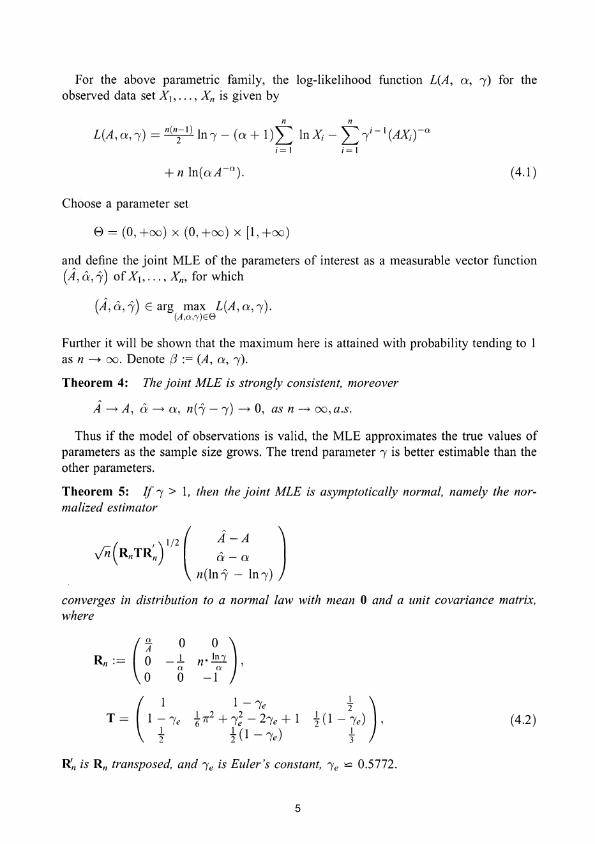
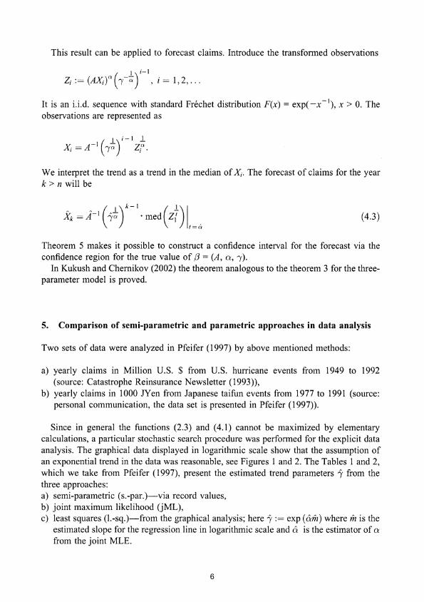
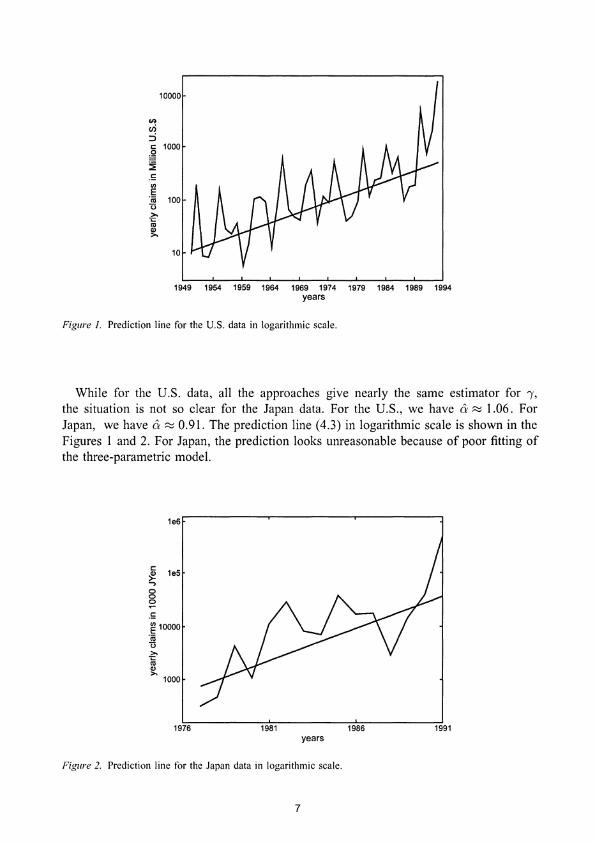
Since in general the functions (2.3) and (4.1) cannot be maximized by elementary calculations, a particular stochastic search procedure was performed for the explicit data analysis. The graphical data displayed in logarithmic scale show that the assumption of an exponential trend in the data was reasonable, see Figures 1 and 2. The Tables 1 and 2, which we take from Pfeifer (1997), present the estimated trend parameters i from the three approaches: a) semi-parametric (s.-par.)-via record values, b) joint maximum likelihood (jML), c) least squares (l.-sq.)-from the graphical analysis; here i := exp (am) where m is the

estimated slope for the regression line in logarithmic scale and a is the estimator of a from the joint MLE.

6

10000

.... en ::i c: ~

1000

~ .S ., E

~ 100

~ 01

~

10

1949 1954 1959 1964 1969 1974 1979 1984 1989 1994 years

Figure 1. Prediction line for the U.S. data in logarithmic scale.

While for the U.S. data, all the approaches give nearly the same estimator for 'Y, the situation is not so clear for the Japan data. For the U.S., we have Ii ~ 1.06. For Japan, we have Ii ~ 0.91. The prediction line (4.3) in logarithmic scale is shown in the Figures 1 and 2. For Japan, the prediction looks unreasonable because of poor fitting of the three-parametric model.

1e6

c: ~ 185 .., 8 o ~

.S ~ 10000

'OJ 13 » 't:

~ 1000

1976 1981 years

Figure 2. Prediction line for the Japan data in logarithmic scale.

1986 1991

7

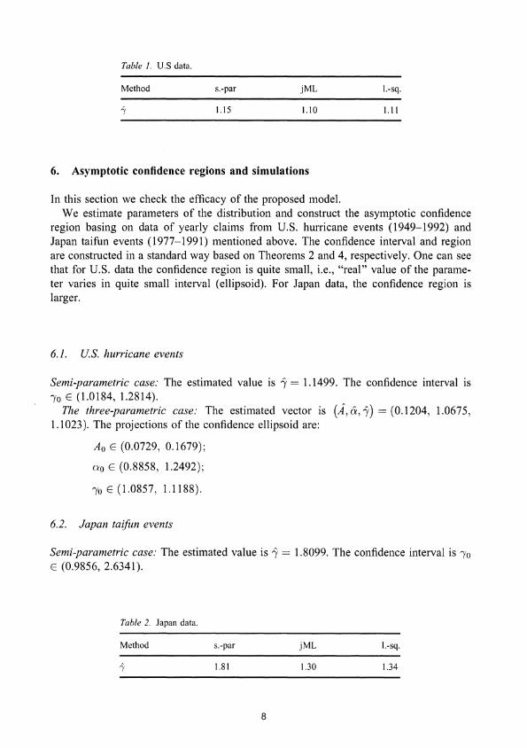
Table 1. U.S data.

Method s.-par jML I.-sq.

1.15 1.10 1.11

6. Asymptotic confidence regions and simulations

In this section we check the efficacy of the proposed model. We estimate parameters of the distribution and construct the asymptotic confidence

region basing on data of yearly claims from U.S. hurricane events (1949-1992) and Japan taifun events (1977-1991) mentioned above. The confidence interval and region are constructed in a standard way based on Theorems 2 and 4, respectively. One can see that for U.S. data the confidence region is quite small, i.e., "real" value of the parameter varies in quite small interval (ellipsoid). For Japan data, the confidence region is larger.

6.1. U.S. hurricane events

Semi-parametric case: The estimated value is i = 1.1499. The confidence interval is )'0 E (1.0184, 1.2814).

The three-parametric case: The estimated vector is (1, eX, i) = (0.1204, 1.0675, 1.1023). The projections of the confidence ellipsoid are:

Ao E (0.0729, 0.1679);

000 E (0.8858, 1.2492);

)'0 E (1.0857, 1.1188).

6.2. Japan taifun events

Semi-parametric case: The estimated value is i = 1.8099. The confidence interval is )'0

E (0.9856, 2.6341).

Table 2. Japan data.

Method s.-par jML I.-sq.

1.81 1.30 1.34

8

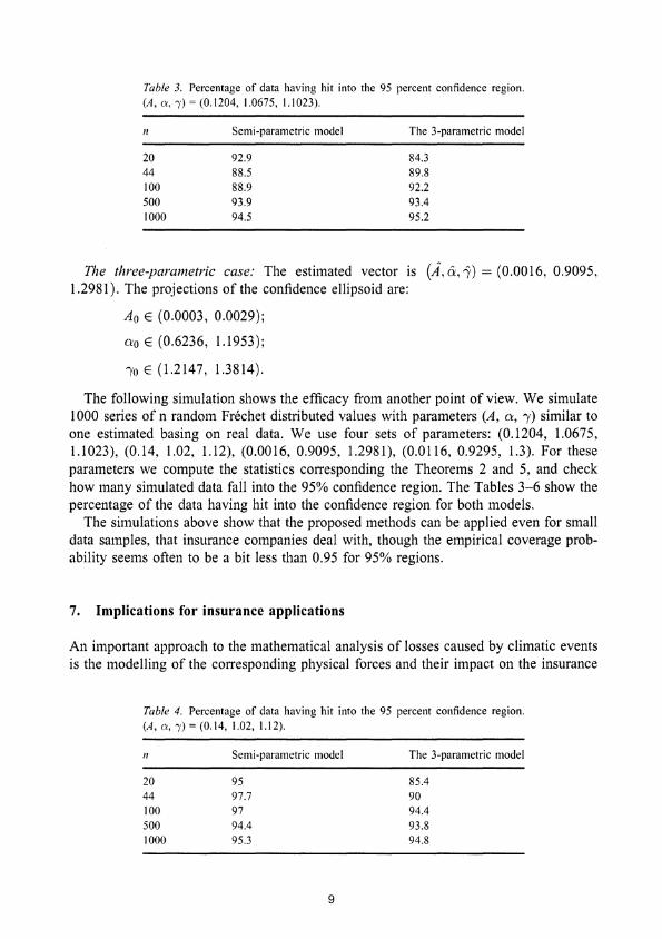
Table 3. Percentage of data having hit into the 95 percent confidence region. (A, 0:, "y) = (0.1204, 1.0675, 1.1023).

n

20 44 100 500 1000

Semi-parametric model

92.9 88.5 88.9 93.9 94.5

The 3-parametric model

84.3 89.8 92.2 93.4 95.2

The three-parametric case: The estimated vector is (1, a, i) = (0.0016, 0.9095, 1.2981). The projections of the confidence ellipsoid are:

Ao E (0.0003, 0.0029);

ao E (0.6236, 1.1953);

1'0 E (1.2147, 1.3814).

The following simulation shows the efficacy from another point of view. We simulate 1000 series of n random Fn!chet distributed values with parameters (A, a, 1') similar to one estimated basing on real data. We use four sets of parameters: (0.1204, 1.0675, 1.1023), (0.14, 1.02, 1.12), (0.0016, 0.9095, 1.2981), (0.0116, 0.9295, 1.3). For these parameters we compute the statistics corresponding the Theorems 2 and 5, and check how many simulated data fall into the 95% confidence region. The Tables 3-6 show the percentage of the data having hit into the confidence region for both models.

The simulations above show that the proposed methods can be applied even for small data samples, that insurance companies deal with, though the empirical coverage probability seems often to be a bit less than 0.95 for 95% regions.

7. Implications for insurance applications

An important approach to the mathematical analysis of losses caused by climatic events is the modelling of the corresponding physical forces and their impact on the insurance

Table 4. Percentage of data having hit into the 95 percent confidence region. (A, 0:, "y) = (0.14, 1.02, 1.12).

n Semi-parametric model The 3-parametric model

20 95 85.4 44 97.7 90 100 97 94.4 500 94.4 93.8 1000 95.3 94.8

9

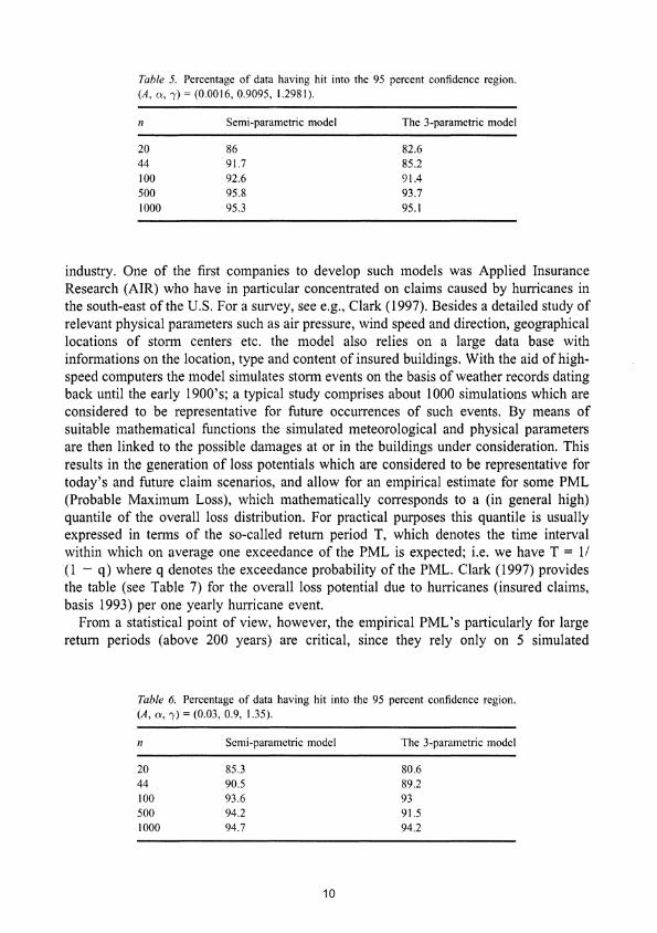
Table 5. Percentage of data having hit into the 95 percent confidence region. (A, 0:, ,,) = (0.0016, 0.9095, 1.2981).


20 86 82.6 44 91.7 85.2 100 92.6 91.4 500 95.8 93.7 1000 95.3 95.1

industry. One of the first companies to develop such models was Applied Insurance Research (AIR) who have in particular concentrated on claims caused by hurricanes in the south-east ofthe U.S. For a survey, see e.g., Clark (1997). Besides a detailed study of relevant physical parameters such as air pressure, wind speed and direction, geographical locations of storm centers etc. the model also relies on a large data base with informations on the location, type and content of insured buildings. With the aid of highspeed computers the model simulates storm events on the basis of weather records dating back until the early 1900's; a typical study comprises about 1000 simulations which are considered to be representative for future occurrences of such events. By means of suitable mathematical functions the simulated meteorological and physical parameters are then linked to the possible damages at or in the buildings under consideration. This results in the generation of loss potentials which are considered to be representative for today's and future claim scenarios, and allow for an empirical estimate for some PML (Probable Maximum Loss), which mathematically corresponds to a (in general high) quantile of the overall loss distribution. For practical purposes this quantile is usually expressed in terms of the so-called return period T, which denotes the time interval within which on average one exceedance of the PML is expected; i.e. we have T = 11 (l - q) where q denotes the exceedance probability of the PML. Clark (1997) provides the table (see Table 7) for the overall loss potential due to hurricanes (insured claims, basis 1993) per one yearly hurricane event.

From a statistical point of view, however, the empirical PML's particularly for large return periods (above 200 years) are critical, since they rely only on 5 simulated

Table 6. Percentage of data having hit into the 95 percent confidence region. (A, 0:, ,,) = (0.03, 0.9, 1.35).


20 85.3 80.6 44 90.5 89.2 100 93.6 93 500 94.2 91.5 1000 94.7 94.2

10

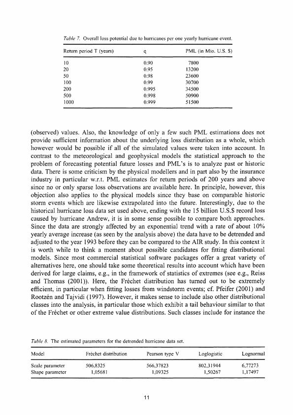
Table 7. Overall loss potential due to hurricanes per one yearly hurricane event.

Return period T (years) q PML (in Mio. U.S. $)

10 0.90 7800 20 0.95 13200 50 0.98 23600 100 0.99 30700 200 0.995 34500 500 0.998 50900 1000 0.999 51500

(observed) values. Also, the knowledge of only a few such PML estimations does not provide sufficient infonnation about the underlying loss distribution as a whole, which however would be possible if all of the simulated values were taken into account. In contrast to the meteorological and geophysical models the statistical approach to the problem of forecasting potential future losses and PML's is to analyze past or historic data. There is some criticism by the physical modellers and in part also by the insurance industry in particular w.r.t. PML estimates for return periods of 200 years and above since no or only sparse loss observations are available here. In principle, however, this objection also applies to the physical models since they base on comparable historic stonn events which are likewise extrapolated into the future. Interestingly, due to the historical hurricane loss data set used above, ending with the 15 billion U.S.$ record loss caused by hurricane Andrew, it is in some sense possible to compare both approaches. Since the data are strongly affected by an exponential trend with a rate of about 10% yearly average increase (as seen by the analysis above) the data have to be detrended and adjusted to the year 1993 before they can be compared to the AIR study. In this context it is worth while to think a moment about possible candidates for fitting distributional models. Since most commercial statistical software packages offer a great variety of alternatives here, one should take some theoretical results into account which have been derived for large claims, e.g., in the framework of statistics of extremes (see e.g., Reiss and Thomas (2001)). Here, the Frechet distribution has turned out to be extremely efficient, in particular when fitting losses from windstonn events; cf. Pfeifer (2001) and Rootzen and Tajvidi (1997). However, it makes sense to include also other distributional classes into the analysis, in particular those which exhibit a tail behaviour similar to that of the Frechet or other extreme value distributions. Such classes include for instance the

Table 8. The estimated parameters for the detrended hurricane data set.

Model

Scale parameter Shape parameter

Frechet distribution

506,8325 1,05681

Pearson type V

566,37823 1,09325

Loglogistic

802,31944 1,50267

Lognormal

6,77273 1,17497

11

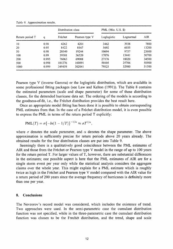
Table 9. Approximation results.

Distribution class PML (Mio. U.S. $)

Return period T q Frechet Pearson type V Loglogistic Lognormal AIR

10 0.90 4262 4201 3462 3938 7800 20 0.95 8422 8167 5692 6035 13200 50 0.98 20340 19244 10694 9757 23600 100 0.99 39381 36520 17076 13441 30700 200 0.995 76063 69088 27176 18020 34500 500 0.998 181276 160091 50105 25706 50900 1000 0.999 349459 302041 79525 32980 51500

Pearson type V (inverse Gamma) or the loglogistic distribution, which are available in some professional fitting packages (see Law and Kelton (1991». The Table 8 contains the estimated parameters (scale and shape parameter) for some of these distribution classes, for the detrended hurricane data set. The ordering of the models is according to the goodness-of-fit, i.e., the Frechet distribution provides the best result here.

Once an appropriate model fitting has been done it is possible to obtain corresponding PML estimates from that. In the case of a Frechet distribution model, it is even possible to express the PML in terms of the return period T explicitly:

PML(T) = a{ -In(l - liT)} -lin ~ aTI/a.,

where a denotes the scale parameter, and a denotes the shape parameter. The above approximation is sufficiently precise for return periods above 20 years already. The obtained results for the four distribution classes are put into Table 9.

Seemingly there is a qualitatively good coincidence between the PML estimates of AIR and those from the Frechet or Pearson type V model in the range of up to 100 years for the return period T. For larger values ofT, however, there are substantial differences in the estimates; one possible aspect is here that the PML estimates of AIR are for a single stonn event per year only while the statistical analysis considers the aggregate claims over the whole year. This might explain for a PML estimate which is roughly twice as high in the Frechet and Pearson type V model compared with the AIR value for a return period of 200 years since the average frequency of hurricanes is definitely more than one per year.

8. Conclusions

The Nevzorov's record model was considered, which includes the existence of trend. Two approaches were used. In the semi-parametric case the cumulant distribution function was not specified, while in the three-parametric case the cumulant distribution function was chosen to be the Frechet distribution, and the trend, shape and scale

12

parameters were estimated simultaneously. Theorems about the consistency of the MLE's are the central results of the paper. They do not follow directly from well-known general properties of MLE, because the considered model is non-regular and contains non-identically distributed observations. The asymptotic normality results are proven as well, and the results about the asymptotic efficiency of the estimators are stated.

It would be interesting to expand the results in parametric setting to other cumulant distribution functions. The model based on Frechet distribution fits the losses from the U.S. hurricanes, but it is not the case for Japanese taifuns. It would be interesting to adapt the Nevzorov's model for Japanese events.

9. Proofs

The following simple lemma gives the way to prove the asymptotic normality. The proof of the lemma is standard and uses Taylor expansion, compare Cramer (1999). One can find it, for example, in Kukush and Chemikov (200 I).

Lemma 1: Let e c Rd , 00 be an interior point of e, {Qn(O), 0 E e, n 2: I} be a sequence of random fields, which are twice differentiable in the neighborhood of 00, Let On be a random vector defined by

On = arg max Qn (0), OEE>

and suppose that On ~ 00 in probability. Assume also that:

a) y'iiQ~(Oo) converges in law to a random vector 'Y, b) Q~ (00) ~ S in probability, where S is nonsingular matrix, c) For each 8 > 0

lim lim sup P ( sup IIQ~ (0) - Q~ (00) II > 8) = O. ,-0 n-+oo 110-0011-<;,

9.1. Proof of Theorem 1

(i) Limit functional. Introduce the normalized log-likelihood function Q,

1 Q = Qnb) := -;;L(,) = Q(n,l) + Q(n,2) ,

with

1 ~ ( 0) Pi Q(n,l) := - ~ Ii - Pi In--n i=2 1 - Pi

(9.1.1)

(9.1.2)

13

and

1 ~ [ 0 Pi ( ] Q(n,2) := - ~ Pi In --+ In 1 - Pi) . n i=2 1 - Pi

(9.1.3)

Then functional Q(n, l)('y) ---+ 0, n ---+ 00 a.s., for each 'Y ;::: 1. Indeed, by the Rosenthal inequality for independent random variables (see Rosenthal (1970» we have

E~ Q1.,.) ,; ':~st (t, In' 1 ~ p; )', '!f~~. E~ (I; - p7)'

< const (~ In2---..EL) 2 - --;;r ~ 1 - p. i=2 I

If 'V > 1 then the sequence In2 ~, i ;::: 2 is bounded, therefore I T=Jii

E n4 < const ,o~(n,l) - ---;:;r-'

If 'V = I then In2....£L.. = In2(i - 1) and I I-Pi '

(9.1.4)

(9.1.5)

E n4 < const In4n. (9 1 6) ,o~(n,l) - n2 ..

By the Chebyshev inequality we have P'o {IQ(n,1) I > 8} ::; Eoo~n.J); hence in both cases (9.1.5) or (9.1.6)

00

L E,oQ(n,l) < 00, n=2

and by the Borel-Cantelli lemma Q(n, I) ---+ 0, n ---+ 00 a.s.

The deterministic part Q(n, 2) converges to the limit

{P?ln 1 '!! Pi + In (1 - Pi), ~f 'Y > I, 'Yo ;::: 1

Qoo("(, 'Yo) = 0, If'Y = 'Yo = 1 or

-00, if'Y=l,'Yo>l.

{(I - 'Yo I) In ("( - 1) - In 'Y, if 'Y > 1, 'Yo ;::: 1

Qoo("(, 'Yo) = 0, if 'Y = 'Yo = I

-00, if 'Y = 1, 'Yo > 1

(9.1.7)

Therefore, for each 'Y ;::: 1

(9.1.8)

14

(ii) Unifonn convergence of Qn. Fix E > 0 and C > 1 + E. For fixed w, the functional sequence

() 1 ~ ( 0) Pi [ 1 Q(n,l) "'I :=-~ Ii-Pi In-1--, "'IE I+E,Cjn::::l, n i=2 - Pi

is equicontinuous, therefore

Then, Q(n,2)b) --+ Qoob, "'10), n --+ 00 unifonnly for "'I E [1 + E, C]. Therefore

(9.1.9)

i.e., we obtain unifonn convergence a.s. for "'I belonging to a bounded interval, separated from 1.

(iii) Maximum point ofQoo. Fonnula (9.1.7) implies directly the contrast inequality:

(9.1.10)

(iv) Behavior ofQnfor large and small "'I. Let"'l:::: C> 1. From (2.2) we obtain

Therefore a.s.

lim lim sup sup Qnh) = -00. C -> + 00 n--+oo "I?C

(9.1.11)

Now, let "'10 > I and "'I S 1 + E, with fixed E > O. Again use (2.2):

n

Qnh) S; k~Ii Inpi(1 + E) --+ (1 - "'10 1) In (1 - (1 + E)-I), n --+ 00 a.s. /=2

Therefore, if "'10 > 1 then

lim lim sup sup Qnh) = -00. f--+O n->oo "1:0; I +f

(9.1.12)

(v) Strong consistency for "'10> 1. Choose no(w), S.t. i < 00 for n :::: no(w). Then for n :::: no(w) we have

15

From (9.1.11), (9.1.12) we get that for some f > 0, C> 0, nl(w)

in E [1 + f, q, for n ~ nl (w). (9.1.13)

If lin(w) - 1'01 ~ 8> 0 and n ~ nl(w), then

Qn(in)::; sup Qnb) = sup Qoob,I'o)+o(I),n->oo. 1')'-')'012': D, ')' E [I + E, C] II' - ')'012': D, ')' E [I + E, C]

Hence

Qoobo,I'o)::; sup Qoo(')',I'o)+o(l). II' -')'012': D, ')'E[I +E, C]

But because of (9.1.10) this can hold only for a finite set of numbers n. Therefore there exists n2 = n2(w), S.t. for all n ~ n2(w), lin(w) - 1'01 < 8. Hence in -> 1'0 a.s.

(vi) Consistency for 1'0 = 1. Similarly in the case 1'0 = 1 we have

in E [1, C], for n ~ nl (w).

If lin(w) - 11 ~ 8 and n ~ nl(w), then

and

Qn(in)::; sup Qnb) = sup Qoo(')', 1) + 0(1), n -> 00, ,),E[I+D,C] ,),E[I+D,C]

Qoo(l, 1)::; sup Qoob, 1) + 0(1). ')'E[I H,C]

From (9.1.10) we obtain again that for n ~ n2(w), lin(w) - 11 < 8.


Here we have 1'0 > 1. We apply Lemma 1.

(i) Convergence of the first derivative. From (9.1.2) we have

~Q' ( ) _ 1 ~ (1 0) p'ibo) yn (n,l) 1'0 - 'n~ i-Pi 0(1_ ?).

Y"i=2 P, P,

(9.2.1)

16

By the CLT in Lyapunov form we get

(9.2.2)

Now, the function

¢(Pi) := p~ln (1 '!! Pi) + In (1 - Pi)

has a minimum point Pi = p?, therefore

..sL¢(Pi) 1 = d~~?) dP:}'YO) = 0 d'Y ')'=')'0 P, 'Y

and

(9.2.3)

Now, (9.2.2) and (9.2.3) imply

(9.2.4)

(ii) Convergence of the second derivative. We have

(9.2.5)

The derivatives in (9.2.5) form a bounded sequence, and using the second moment one can easily show that

Q[~,I)C'YO) -+ 0 in probability P,),o'

Now,

d2:$i) 1,),=,),0 = ¢"(p~)(pIC'Yo)/ + ¢' (pnp;' C'Yo) = ¢"(p~)(p:C'YO))2,

and ¢" (p?) = 0 (1 0)' Then Pi I-Pi

lim d2¢(Pi) I = -lim Wi C'Yo) ): = i-oo dy. ')'=')'0 ;-00 Pi (1 - Pi)

(9.2.6)

17

Therefore

}i.l~,Q(~,2)bo) = '"Y02b! - 1)" (9.2.7)

Finally, (9.2.6) and (9.2.7) imply the convergence

2 (1 ) in probability P "(0. '"Yo '"Yo - 1

(9.2.8)

(iii) Oscillations of Q~'. Fix E > 0, C> 1 + E. From (2.2) we get for '"Y E [1 + E, C]

n n

Q';' b) = *'L,Mlnpi)'" + *'L, (In (1 - Pi))"'(1 - Ii), i=2 i=2

and there exists a constant M, s.t. for all n ~ 1, all '"Y E [1 + E, C]

IQ~'b)1 ~M. (9.2.9)

Now we are able to apply the above mentioned Lemma 1.

..fii(i - '"Yo) --> '"Y5bo - l)N( 0, '"Y~bol- 1))

= N (0, '"Y5 bo - 1)) in distribution. (9.2.lO)


(i) Reparametrization. We prove the statement of the theorem using the notation (3 = (30 = (Ao, 0:0, '"Yo). ~~t Bo = AoQO , B = A-Q , ~o = In ;rq ~. 0, /-1 = In '"Y. Rewrite th~ function (4.1) usmg the Ll.d. sequence Zi = (AoXi) 0 ('"Yo I) , I = 1, 2, ... , and cancellmg summands which do not depend upon B, a, /-1. We get

Q

Now, let c = BB~QO = (~)", T =::. ,1/ = /-1- ::0/-10. Rewrite LI and cancel the summands which do not depend upon the new arguments:

n(n _ 1) n n L2 (c, T, 1/) = ~1/ + n Inc + n In T - T'L, lnzi - c'L, eU- I )vzj7.

i=l i=l

18

Now, E In z\ = -r/(1) = "Ie, see Kukush and Chemikov (2001), EzIT = r(l + T). Then

n

~L2(C, T, v) = yv + (Inc + In T - T"Ie) - ~r(l + T) L e(i-\)v + R\ + R2, ;=\

where

n R\ = -iiL (lnz; - E lnz;),

;=\

n

R2 = -~Le(i-\)V(ZiT -EziT). ;=\

Finally, let ¢ = nv. Rewrite L2:

L3(C, T, ¢) = ~L2 (c, T,*) = n~ l¢ + (Inc + In T - T"Ie)

-~r(l +T)~+R\ +R2. en - I

(9.3.1 )

(9.3.2)

(9.3.3)

For ¢ = 0 we assume here and further formally that ~ e~-I = 1. A new parameter set is en -\

e = {(C,T,¢): 0 < c < 00,0 < T < oo,¢ E R}.

Denote (c,f,¢) = argmaX(C,T,q,)ESL3(c,T,¢). Obviously, if¢ 2:: -n!ln"lo then

c= (1)&' f=:}o, ¢=n(lni-:}oln"lo), (9.3.4)

The true value 130 corresponds to the values Co = TO = 1, ¢o = O. We must prove, that a.s. in P,80

(c, f, ¢) ~ (co, TO, ¢o), as n ~ 00.

(ii) Limit function. Consider (c, T, ¢) E eR, where eR is a compact subset of e. Uniformly in eR we have

with the limit function

Loo(c, T, ¢) =! + Inc + In T - rye - cr(l + T)-¥.

19

Here for ¢ = 0 we assume that eO;l = I. The function L3(c, T, ¢) converges to Loo(c, T, ¢) uniformly a.s., when (c, T, ¢) E eR. Looking at (9.3.3), it is enough to prove that with probability 1 R] and R2 converge to 0 uniformly, n - 00, when (c, T, ¢) E eR•

R] converges to 0 uniformly a.s., because ~L 7=1 (lnz; - E lnz;) - 0 a.s. by SLLN. To prove that R2 converges to 0 uniformly a.s., it is enough to prove that

S (,i..) n (i-1 )¢ n ,+" T _ 1 ~ ( -r _ E -r) n -nL..J e n z; z;

;=1

converges to 0 uniformly a.s. One can use the 4-th moment and the Rosenthal inequality (Rosenthal, 1970), the Chebyshev inequality and the Borel-Cantelli lemma to obtain that s,(t,r) -> 0, n _ 00 a.s., for all ¢, T. Uniform convergence a.s. follows from the relations:

1 8Sn(¢,T) _ l~i-l (i-I)¢( -r E -r) and n a¢ -nL..J-n- e n z; - z; ,

;=1

sup sup Ik 8Sn~' T) I ::; C(w); n2':1 ¢,rEcompact

the same for

(iii) Loo attains its maximum at the unique point (co, TO, ¢o) = (1, 1, 0). Find the maximum point of Loo. We have

8f;go =! - r(1 + T)e<l> ;- 1.

If the maximum of Loo exists then it is attained on the curve 8f;go = 0, or

( <I> )-' c= r(1 +T)Y .

Consider Loo on this curve,

Loo(T, ¢) = Loo(c(T, ¢), T, ¢) = -lnr(1 + T) -In e¢;- 1 + In T - T "Ye + ~ - 1.

Prove that g( ¢) := ~ - In e<l> ;- 1 attains the maximum at the unique point ¢ = 0: g(0) = O. Indeed,

g(¢) := ~ -lny::; 0 {:} y ~ e~ {:}

{:} [h = e<l> - ¢A - 1 ~ 0, ¢ ~ 0 ,

1!. h = e¢ - ¢e2 - 1 ::; 0, cj; < 0

(9.3.5)

20

g(O) = 0. We have

I ,/, !P.. c/J!P.. !P.. c/J h = e'f' - e 2 -1"e2 2:: 0, as e 2 2:: 1 + 1"' for all ¢ E R.

Equality holds here only for ¢ = 0. Therefore, the only maximum point of g is zero. We have to prove that the function/(r) := lnr - lnf(1 + r) - r'Ye, r> ° has the

unique maximum point r = 1. Consider the inequality

In r -lnf(1 + r) - rye::; -'Ye ¢:} lnr(r) 2:: (1 - rhe.

But the function In r(r) is strictly convex, and y = (r - 1)r'(l) is a tangent line to the graph y = In r(r) at the point r = 1. Therefore, for r of:. 1 lnr(r) > (1 - r)'Ye, and the only maximum point of/is r = 1. So, we proved that the only maximum point of Loo is (1, 1, 0).

(iv) iJ is stochastically bounded. Consider the transformed function given in (9.3.3)

n . !p.. L3(C, r, ¢) = ~(1 - -k) + (Inc + In r - r 'Ye) + RJ - #2: e(I-J)nziT,

I

c > 0, r > 0, ¢ E R, and find the curve on which it attains its maximum upon c:

oL3 _l_l~e(i-I)!p.. -T-O oc - c nL..t nZi - , I

and c = n J . Consider first the case ¢ 2:: 0. On this curve the function equals '""' n (i~l -1" L.Jle nZi

L3(r, ¢) = L3(c(r, ¢), r, ¢) = ~(1 - -k) -In (-k~ e(i-I)~ziT) + In r - r 'Ye

+ RJ - 1 < ~(1 - -k) -In (-kif t ZiT) + lnr - r 'Ye+RI, [23n] +2

L3(r, ¢) < -fn- -t -In (-k 2: ZiT) + In r - rye+ RI z· < e"(e-2 [l!!.] +2<i<n

I '3 --

(9.3.6)

Remind that {Zi} are i.i.d. realizations of a Frechet distribution with

F(x) = exp( -X-I), x> 0, P{Zi < e'Ye - 2} = exp( -exp( -'Ye + 2)) := p.

(9.3.7)

21

Denote by Vn/3 the number of Zi such that Zi < e'Ye-2 , [~] + 2 ~ i ~ n. Then by SLLN ;;n. -> p, as n ~ 00, a.s. So, we obtain that for any 0 < lOl < P there exists no = no(lO], w) such that for

any n > no I~ - pi < lOl, a.s., therefore Vn/3 > ~ (-lOl + p) a.s. Also we have that a.s. for n > no

L3(r, cjJ) < In r - r 'Ye - ~ + RI - 2r + r 'Ye -lnt( -El + p)

= In r - 2r - * -CI + R1• n

RI = -i2: (lnz; - Elnzi) i=1

~ rklt (lnzi - ElnZi)l· I-I

There exists a number n2 = n2(w) such that ~IE7-1 (lnzi - Elnzi) I < 1 a.s., as soon as n > n2(w).

Therefore for any n > no = max(nl. n2)

L3 ( r, cjJ) < In r - r - * -C 1

Also we have

sup sup sup L3(r,cjJ) ~ -00 a.s. when C' ~ +00, n>nu T>c' 4;;::0

sup sup sup L3 (r, cjJ) -> -00 a.s. when {j -> 0, n>no T < 6 ¢:2:0

sup sup sup L3(r, cjJ) -> -00 a.s. when C' -> +00. n>nu T>O ¢>C'

Similarly consider the function L3 ( r, cjJ) when cjJ < 0:

(9.3.8)

(9.3.9)

22

Denote by v:'/3 the number of Zi such that Zi < e7e - 2 , 1 ::; i ::; [~l + 1 .

Then by SLLN ~ -'0 p, as n ---+ 00, a.s., where p is given in (9.3.7) . • /3 I ' I For any 0 < £] <p there exists no = nO(£h w) such that for any n > no 7$-P < EI, a.s.,

therefore V~/3 > j( -£] + p) a.s. And we have that a.s. for n > no

13(T, ¢) < lnT - T "'Ie +~ - fn+R] - 2T + T "'Ie -ln~(-£I + p)

= lnT - 2T+~-fn- CI +Rl.

RI = -fit (lnzi - E1nzi)::; T-klt (lnzi - ElnZi)l· I-I i-I

For any £2 > 0 there exists n2(£2, w) such that for any n > n2 ~1L:7-1 (lnzi - ElnZi) \ < £2 a.s. Let £2 = 1. There exists a number n2 = n2(w) such that ~ I: i-I (lnzi - E1nzi) I < 1 a.s., as soon as n > n2(w). Therefore for any n > no = max(nh n2, 6)

Also we have

sup sup sup 13(T, ¢) ---+ -00 a.s. when C' ---+ +00, n>no r>C' r/> < 0

sup sup sup 13 (T, ¢) ---+ -00 a.s. when 8 ---+ 0, n>no r>C r/>< 0

sup sup sup 13(T, ¢) ---+ -00 a.s. when C' ---+ +00. n>no r>O r/> < -C'

(9.3.10)

Since Ln(On) ;::: Ln(Oo) = Loo(Oo, ( 0) + 0(1), n ---+ 00, from (9.3.8) and (9.3.10) we can conclude that for some random bounds 0, C> 0 and some number no(w) for each n ;::: no(w)

On E [8, q X [8, q X [-C, q, a.s. (9.3.11 )

(v) Convergence of (c,f,J;).

From (9.3.11) we get that 11011 ::; a , with a = a(w) for n ;::: no(w). Then for n ;::: no(w)

L3(0)::; SUpL3(O) = sup Loo(O) +0(1). 11811:$a 118119

23

2 2 (A )2 If (c - co) + (f - TO) + </J - </JO ~ 82, then

sup Loo(O) ~ Loo(Oo) + 0(1), (C-co)2 +( T-TO)2 +( ¢-¢o f ?62, 11811:5a

and for n ~ nl(w) this is impossible, because of (iii). Hence (c - cO)2 + (f - To)2 + (¢ - </JO)2 ~ 82 , n ~ nl(w) and therefore (c, f, ¢) --->

(co, TO, </Jo) a.s., n ---> 00. Now from (9.3.4) the statement of Theorem 3 follows.


We apply Lemma 1 to Qn = L3 given in (9.3.3), (9.3.1) and (9.3.2) with 0 = (c, T, </J), e = (0, 00) x (0, 00) x Rand 00 = (co, TO, </Jo) = (1, 1,0). Rewrite

L3(C,T,</J) = Loo(C,T,</J) +An(c,T,</J) +Rl +R2 -fn, (9.4.1 )

where AnCc, T, 0) = 0 and in the case </J * 0

An(c,T,</J)=Cr(l+T)(e¢-l)(i- fl ). n(en - 1)

By Theorem I the maximum point (c, f, ¢) of L3 converges to 00 = (co, TO, </Jo) a.s. We check the conditions of Lemma 1.

(i) Convergence of /iiQ~(eo). We have J.joo(Oo) = O. Consider An with t := * ' An(c,T,</J) =cr(l +T)(e¢ i I) (1- el ~ J.

Let h(t) = 1 - e'~1 if t * 0, and h(O) = O. Then

BAn ( ( 0 ) ( ) 8 () I 1 I () 1 B</J = cor 1 + TO 8¢h t 1=0 = nh 0 = Tn'

Therefore /ii8A'l);t0) ---> O. The other partial derivatives of An equal zero at 00, Thus /iiQ~((Jo) = 0(1) + /ii(R I +R2)'((JO),

( z:-I - Ez:-I ) 1 n I I

v'nQ~(eo)=o(1)- /iif= (l-zjl)lnzi-E(l-zjl)lnzi . I-I I-I (-I E -I) - z· - z· n I I

Now by the multivariate CLT in Lyapunov form

v'nQ~(Oo) ---> N(O, T)

(9.4.2)

(9.4.3)

24

in distribution, where T is 3 x 3 matrix. Check the Lyapunov condition for the third component (9.4.2). For the sum

n n

S '" t' '" i-I (-I E -I) n = ~ <"ni = ~ r.; zi - Zi i=1 i=1 nyn

we have

1 ~ (i - 1)2 1 Var Sn = n~ 2 ~ j' n ~ 00,

i=1 n

and

To calculate the variance-covariance matrix T, introduce the i.i.d. random vectors

and weighting matrices

A '-d' (1 Ii-I) i·- lag, '-n-'

Then vnQ~((Jo) = 0(1) - )nL:7=1 Ai~i'

1 -,e i2 2 6+ (1 - re)

1 - re

1 - re

i2 2 1 - re 6 + (1 - re)

1 - re 2 2

This T is the covariance matrix of the normal law in (9.4.3).

2

1 - re 2 1

3

(ii) Convergence of Q~((Jo). Direct calculations show that L~ - T. This matrix is nonsingular because det T = i2 + i2(r" (2) - (r' (2) )2) > O. Here r' (2) = 1 - re, r"(2) = t + r; - 2re , see, e.g., Abramowitz and Stegun (1992). The second derivatives of the

25

other summands in (9.4.1) tend to zero in probability, hence Q~(Oo) ---+ S = -T in probability.

(iii) Increments o/the second derivative. For the limit function we have Loo(c, T, cf;) E

C2(e), therefore condition c) of Lemma 1 holds if we substitute Loo for Qn. For the other summands of (9.4.1) it is also simple to check this condition. Consider for instance the increments with respect to cf; of

2 n ( . 1)2 (i - I)</> 8 ~2 __ £ '" I - n ( -T _ E -T)

!Cl", - n~ 2 e Zi Zi' U'f' ;=1 n

We have to check that for each /) > 0,

lim lim sup P sup *2:: I 2 e n - 1 (ZiT - EZiT) > 8 = O. ( I n C- 1)2( (i-l)</» I) <->0 n->oo OEe, i= I n

110-0011:'0<

(9.4.4) The following inequalities hold:

e n - 1 :<:::; I -;; IE • const, when Icf; - cf;ol = 1cf;1 :<:::; 10; I (i - 1 )</> I .

{ -1/2' f 1 zi ,1 Zj>

IZiTI :<:::; Zi* = when IT - Tol = IT - 11:<:::; i· -3/2 'f 0 . 1 Zi ,1 < Zj:<:::; ,

Hence the supremum in (9.4.4) is less or equal to 10 • OP(I), and

lim lim sup P(E . Op(l) > 8) = 0, €----1-0 n-+oo

which induces (9.4.4). Condition c) of Lemma 1 holds.

(iv) Change o/variables. By Lemma 1

Vn(;~:) ~ T-'F (~ in law, with , ~ N(O, T), and soo ~ N(O, T-'). Return to the variables (A, a, ,). We have

( Aoc_...L ) (lOT

aoT :=g(c,T,cf;), cf; + Tln,o

26

and

( ~~ ) =g(l,l,O). n In 'Yo

The nonnalized estimators equal

( A -Ao ) Vn a-ao =Vn(g(c,f,¢)-g(l,l,O))

n(1n i-In 'Yo)

(C-l) = Vng'(I, 1,0) f J 1 + op(l) - g'(I, 1, OKlO (9.4.5)

in law. But

(g'(I, 1,0)) -1 = h'(Ao, ao, n In 'Yo), (9.4.6)

where the inverse transfonnation h equals

( (A/Ao)-a )

h(A,a,c/» = a/ao . 'IjJ - an In'Yo/ao

Then

(9.4.7)

with Rn given in Theorem 2, R~ is Rn transposed. Finally, from (9.4.5)-(9.4.7) we obtain that the sequence

converges in law to standard nonnal distribution.

27

Acknowledgments

Alexander G. Kukush was supported by the DFG under Grant No. 436 UKR 17/29/96 and by INTAS 99-0016. Yuri V. Chemikov was supported by the University of Oldenburg, Gennany. Dietmar Pferifer was supported by AON Jauch & Hiibener, Hamburg. The research was partially realized when Alexander G. Kukush was visiting University of Hamburg, and Yuri V. Chemikov was visiting University of Oldenburg. The authors would like to thank an anonymous referee for valuable comments.

References

Abramowitz, M. and Stegun, I. A., (eds), Handbook of mathematical functions with formulas. graphs. and mathematical tables, Dover Publications, Inc., New York, 1992.

Borovkov, K. and Pfeifer, D., "On record indices and record times," J. Stat. Plann. In! 45, 65-79, (1995). Catastrophe Reinsurance Newsletter, No.2 (1993),8 p. Clark, K.M., "Current and potential impact of hurricane variability on the insurance industry," in Hurricanes.

Climate and Socioeconomic Impacts (H.F. Diaz and R.S. Pulwarty, eds), Springer, New York, 273-283, (1997).

Coles, S., An Introduction to Statistical Modeling of Extreme Values, Springer, London, 2001. Cramer, H., Mathematical Methods (if Statistics. Princeton University Press, Princeton, 1999. Ibragimov, LA. and Has'minskii, R.Z., Statistical Estimation, Asymptotic Theory, Springer, New York-Berlin,

1981. Kukush, A.G., "On maximum likelihood estimator in a statistical model of natural catastrophe claims," Theory

of Stoch. Proces. 5(21),64-70, (1999). Kukush, A.G. and Chemikov, Y.V., "Goodness-of-fit test in Nevzorov's model," TheOl:V of Stach. Proces.

7(23), 203-214, (200 I). Kukush, A.G. and Chemikov, Y.V., "Efficiency of maximum likelihood estimators in Nevzorov's record

model," in Proceedings of the Ui.7'.ainian Mathematical Congress-200!, Kyiv, August, 2001. Probability TheOlY and Mathematical Statistics. Section 9, Kyiv, 85-93, 2002.

Law, A.M. and Kelton, W.O., Simulation Modeling and Analysis, McGraw-Hill, New York, 1991. McNeil, A.J. and Saladin T., "Developing scenarious for future extreme losses using the peaks-over-threshold

method," in Extremes and Integrated Risk Management (P. Embrechts, ed), UBS Warburg Books, London, 255-267, 2000.

Nevzorov, V.B., "Records," Theory Probab. Appl. 32,201-228, (1988). Pfeifer D., "A statistical model to analyse natural catastrophe claims by mean of record values," in Proceedings

of the 28 International ASTIN Colloquium, Cairns, Australia I 0-12 August, 1997, The Institute of Actuaries of Australia, 1997.

Pfeifer, D., "Extreme value theory in actuarial consulting: windstorm losses in central Europe," in Statistical Analysis of Extreme Values, with Applications to Insurance, Finance. Hydrology and Other Fields (R.-D. Reiss and M. Thomas, eds), Birkhauser, Basel, 373-378, (2001).

Reiss, R.-D. and Thomas, M., Statistical Analysis of Extreme Values. with Applications Insurance. Finance. Hydrology and Other Fields, Birkhauser, Basel, 2001.

Rootzen, H. and Tajvidi, N., "Extreme value statistics and windstorm losses: a case study," Scandinavian Actuarial Journal 97, 70-94, (1997).

Rosenthal, H.P., "On the subspaces of L" (p > 2) spanned by sequences of independent random variables," Isr. J. Math. 8,273-303, (1970).

Smith, R. and Goodman, D., "Bayesian risk analysis," in Extremes and Integrated Risk Management (P. Embrechts, ed), UBS Warburg Books, London, 235-250, 2000.

28

Documents

Maximum Likelihood Estimators in a Statistical Model of