Maximum Likelihood Pedigree Reconstruction using Integer Linear

Maximum Likelihood Pedigree Reconstruction using

Integer Linear Programming

James Cussens1, Mark Bartlett1, Elinor M. Jones2, and Nuala A. Sheehan2

1Department of Computer Science, University of York, York, North

Yorkshire, YO10 5GH, United Kingdom

2Department of Health Sciences, University of Leicester, Leicester,

Leicestershire, LE1 6TP, United Kingdom

Running Title: Pedigree Reconstruction using ILP

Corresponding Author: Dr Nuala Sheehan,

Department of Health Sciences,

University of Leicester,

Adrian Building, University Road,

Leicester, LE1 7RH

Tel: 00 44 116 229 7271

Email: [email protected]

1

Abstract

Large population biobanks of unrelated individuals have been highly successful in

detecting common genetic variants affecting diseases of public health concern. However,

they lack the statistical power to detect more modest gene-gene and gene-environment

interaction effects or the effects of rare variants for which related individuals are ideally

required. In reality, most large population studies will undoubtedly contain sets of

undeclared relatives, or pedigrees. Although a crude measure of relatedness might

sometimes suffice, having a good estimate of the true pedigree would be much more

informative if this could be obtained efficiently. Relatives are more likely to share

longer haplotypes around disease susceptibility loci and are hence biologically more

informative for rare variants than unrelated cases and controls. Distant relatives are

arguably more useful for detecting variants with small effects since they are less likely to

share masking environmental effects. Moreover, the identification of relatives enables

appropriate adjustments of statistical analyses that typically assume unrelatedness.

We propose to exploit an integer linear programming (ILP) optimisation approach

to pedigree learning, which is adapted to find valid pedigrees by imposing appropriate

constraints. Our method is not restricted to small pedigrees and is guaranteed to return

a maximum likelihood pedigree. With additional constraints, we can also search for

multiple high probability pedigrees and thus account for the inherent uncertainty in

any particular pedigree reconstruction. The true pedigree is found very quickly by

comparison with other methods when all individuals are observed. Extensions to more

complex problems seem feasible.

Keywords: Constraint based optimisation, Genetic marker data, Bayesian networks,

Model uncertainty

2

1 Introduction

Identification of relatives amongst a group of individuals from genetic marker data is relevant

to areas as diverse as evolution and conservation research, epidemiological and genealogical

research, and forensic science identification problems [Blouin, 2003; Jones and Ardren, 2003;

Meagher and Thompson, 1987; Olaisen et al., 1997]. In medical research, large population

biobank studies of unrelated individuals have been set up worldwide to investigate the ge-

netic risk factors underlying the common complex diseases of major public health concern. It

is now well understood that they do not have sufficient statistical power to detect the effects

of rare genes and the more modest effects of gene-gene and gene-environment interactions.

Sets of relatives are more likely to share longer haplotypes around susceptibility loci and are

hence biologically more informative for rare variants than unrelated ‘cases’ and ‘controls’. In

fact, distant, rather than close, relatives are more likely to be useful for detecting genes with

small effects as the genetic effects are less likely to be masked by the shared environment

effects typically arising in near relatives. In the absence of exact information, general pair-

wise relatedness, rather than specific relationships, can be estimated from population sample

data using approaches based on identity by descent (IBD) methods [McPeek and Sun, 2000;

Sieberts et al., 2002; Leutenegger et al., 2003; Stankovich et al., 2005; Browning and Brown-

ing, 2010; Powell et al., 2010; Thompson, 2008b]. Such methods are particularly efficient at

detecting misspecified relationships: assessing the true relationship is more difficult. How-

ever, large population studies undoubtedly contain pedigrees (i.e. family trees) [Thompson,

2008a] so if it were possible to reconstruct (extended) pedigrees easily from population sam-

ple genetic data, we would have far richer information and sets of distant relatives could be

readily proposed.

Pedigree information is also relevant to standard statistical association testing where fail-

ure to take account of existing relationships can yield overly high false positive results [New-

man et al., 2001; Stankovich et al., 2005; Choi et al., 2009; Thornton and McPeek, 2010].

Likewise, some ‘true’ associations could be missed: a susceptibility gene for which different

variants are segregating in different groups of relatives would never be detected in an asso-

ciation analysis on unrelated individuals. Moreover, even in linkage analyses where pedigree

3

data are required, undeclared relatedness amongst the founders of a particular family and

between founders of different families can heavily bias the results if appropriate adjustments

are not made [Genin and Clerget-Darpoux, 1996; Sheehan and Egeland, 2008; Thompson,

2008a].

It is sometimes convenient to consider the pedigree identification problem as one of de-

termining the most likely pedigree from a set of possible alternatives. In theory, estimating

the most likely pedigree for a given set of individuals from genetic marker data simply

requires consideration of all possible relationships amongst them and computing the like-

lihood for each [Cannings and Thompson, 1981; Thompson, 1975]. However, due to the

potentially enormous number of possible pedigrees, simple enumeration rapidly becomes im-

practical [Egeland et al., 2000; Sheehan and Egeland, 2007]. When general features of the

pedigree are of more interest than precise estimation of the entire set of relationships, ‘se-

quential’ (i.e. greedy) algorithms can be used which produce a single high likelihood (but

not necessarily maximum likelihood) reconstruction by starting from a position where all

individuals are assumed to be unrelated and gradually accepting sibships on the basis of

the increase attained in log-likelihood [Thompson, 1976a]. In order to give good results,

the above approach requires information on age (or at least an age ordering), sex, average

sibship size, typical generation gap and age disparity among parents. Other approaches

to pedigree reconstruction which produce a high likelihood pedigree include simulated an-

nealing [Almudevar, 2003; Riester et al., 2009] and Markov chain Monte Carlo (MCMC)

methods [Almudevar, 2007].

In contrast, the method presented in this paper will yield a guaranteed maximum like-

lihood pedigree, rather than just a high-probability pedigree. This has also been achieved

through Bayesian network learning using dynamic programming by Cowell [2009]. The ap-

proach we propose in this paper uses constraint based methods which have been used for

Mendelian consistency checking [Sanchez et al., 2008] but not to our knowledge for pedigree

reconstruction. More specifically, we use integer linear programming (ILP) to search for

maximum likelihood pedigrees. For clarity and direct comparison with Cowell [2009], we

have chosen to cast the problem as one of Bayesian network learning noting that while this

is not necessary for the situation presented here, such a representation will undoubtedly be

4

useful for more complex applications.

There is no guarantee that the most probable pedigree is the true pedigree [Thompson,

1976b]. This is due to the probabilistic nature of genetic inheritance whereby marker data

on unrelated individuals may indicate that they are, in fact, related and where the observed

data could assign higher likelihood to an incorrect relationship than the true one. Failure

to acknowledge such inevitable uncertainty could lead to spuriously confident inferences and

so, in addition to finding the most likely pedigree, we will also show how our approach can

be used to search for many high likelihood pedigrees.

The structure of the paper is as follows. In Section 2, we outline how a pedigree can be

represented as a Bayesian network and present the likelihood function to be optimised. We

then explain how the pedigree reconstruction problem can be encoded as an ILP optimisation

following the argument presented in Cussens [2010]. Results for this encoding are given for

a straightforward situation in Section 3 and compared with competing methods. The paper

concludes in Section 4 with a discussion of the issues and challenges for future work, including

possible extensions to more complex problems.

2 Material and Methods

2.1 Pedigrees and Bayesian networks

A pedigree can easily be represented as a directed acyclic graph (DAG) [Lange and Elston,

1975], where each node corresponds to a pedigree member and a directed connection (i.e.

arrow, or directed edge) between two individuals represents a parent-child relationship. We

note that this defines a special class of DAG with well defined structural constraints: each

node in the graph is known to have exactly two parent nodes (although either may be latent)

and these parents must be of opposite sexes. A node with no parents is a pedigree founder.

Figure 1(a) shows a simple pedigree in conventional ‘family tree’ form, with males represented

as squares and females as circles. The corresponding DAG is shown in Figure 1(b) and the

marriage node graph [Thomas, 1985; Cannings et al., 1978] in Figure 1(c).

[Figure 1 about here.]

5

A Bayesian network (BN) is a directed acyclic graph whose nodes, v ∈ V , represent

random variables. There are several ways of expressing a pedigree as a BN [Lauritzen

and Sheehan, 2003] but one of the simplest is to consider the graph in Figure 1(b) where

the nodes no longer represent the pedigree members themselves but random variables that

assign genotypes to these individuals. These random variables have a joint distribution that

depends on the pedigree structure and the mode of inheritance for the relevant genetic locus

which can be factorised into a product of conditional distributions for each node given its

parent nodes.

We will introduce our reconstruction approach with a focus, as other authors have done,

on the most straightforward case [Almudevar, 2003; Cowell, 2009; Thompson, 1976a]. Specif-

ically, we assume that the sample of individuals is complete by which we mean that each

observed individual has fully observed genetic data and each unobserved parent is assumed

to be unrelated to any other individual in the sample and is hence an unobserved pedigree

founder. We will also adopt the common assumption of random union of gametes indicating

that founder genes are independent of each other with the consequent implication of Hardy-

Weinberg proportions for founder genotypes. Finally, we will assume that genetic markers

at the different loci under consideration are segregating independently. While perfectly ad-

equate for the independent marker data that we consider here, we note that the above BN

representation of a pedigree will not suffice for more complex genetic models involving linked

loci, for example, where more general graphical model representations are more appropriate.

We note that it also implicitly assumes simple Mendelian inheritance of genes in offspring

from parents [Lauritzen and Sheehan, 2003].

For a given pedigree graph, G, let V be the set of individuals and identify v ∈ V with a

random variable Gv assigning a genotype at a single locus to v. Let fv and mv be the labels

of the nodes representing the father and mother of v, respectively. Then

τ(gv | gfv, gmv

) ≡ P (Gv = gv |Gfv= gfv

, Gmv= gmv

)

denotes the probability that v has genotype gv given the parental genotype combination

of gfvand gmv

. In the event where only one parent, e.g. mv, is observed, we assume that

6

the unobserved parent is a founder and sum over all possible genotypes for that parent.

Specifically,

τ(gv | gmv) =

∑

gfv

τ(gv | gfv, gmv

)p(gfv)

where p(gfv) — the marginal probability that a founder individual fv has genotype gfv

—

is derived from the population allele frequencies and the assumption of Hardy-Weinberg

proportions. This is equivalent to assuming that the gene inherited from the unobserved

parent is randomly drawn from the population allele frequency distribution. In general, we

can express these probabilities as

τ(v, Pa(v,G))

where Pa(v,G) denotes the parent set of v in G which will comprise 0, 1 or 2 nodes and

where τ(v, ∅) ≡ p(gv) represents the marginal probability that v has genotype gv. Note

that these probabilities are just the usual Mendelian transmission probabilities of 0, 1

4, 1

2

or 1 for non-founding pedigree members with two observed parents. Since a pedigree is

completely specified by parent-child relationships, the probability of any single configuration

of genotypes on a pedigree, and hence the likelihood under the assumption of a complete

sample and Mendelian inheritance, decomposes into a product of conditional probabilities

and can be written as

L(G) =∏

v∈V

τ(v, Pa(v,G)). (1)

Note that this is precisely the form of the standard decomposition of a pedigree likelihood

into triplet products under the same assumptions. (See Thompson [2000], for example.)

The aim of a maximum likelihood pedigree reconstruction is to find G such that L(G) is

maximised. Given that the factorisation of the joint distribution in (1) defines a Bayesian

network [Lauritzen, 1996], this is equivalent to searching for an optimal Bayesian network

where the search is constrained to find networks that are valid pedigrees. It is often more

convenient to work with the log-likelihood so our optimisation problem in that case is to find

7

G to maximise

l(G) = log L(G) =∑

v∈V

log τ(v, Pa(v,G)). (2)

Since our multilocus genotype is based on independently segregating markers, by as-

sumption, the joint likelihood of interest is simply a product of likelihoods (Equation (1))

calculated for each locus separately and the log-likelihood is a sum of the relevant expres-

sions (Equation (2)). For convenience, we will thus focus on a single locus to describe our

approach.

2.2 An ILP formulation for likelihood maximisation

An integer linear program (ILP) is defined by:

1. a set of variables X, representing unknown quantities, some of which will be restricted

to take only integer values,

2. a linear objective function of the form∑

x∈X cxx where the coefficients cx are fixed

constants, and

3. linear equations and inequalities putting joint constraints of the form∑

x∈X axx ≤ b

on the values the variables can take where the values ax and b are fixed constants.

The ILP optimisation problem is to find an assignment of values to the variables which

maximises the objective function while respecting all constraints. This is an NP-hard prob-

lem in the general case [Karp, 1972] which means there is no known polynomial time algo-

rithm to solve it in the general case. It is however still possible to solve the problem exactly,

thus guaranteeing that the optimal pedigree is found. One simple algorithm that does so

is to enumerate all potential solutions and examine them in turn. This would of course be

impractically slow for any reasonably sized problem.

Decades of research (both academic and commercial) have gone into creating highly opti-

mised ILP solvers based on the simplex algorithm which achieve good temporal performance

in practice [Wolsey, 1998]. Given increasingly large problems, these solvers will eventually

8

run out of computer memory or take too long to be of practical use. However, provided that

the solvers are given sufficient time and resources, it can be guaranteed that they will always

find the optimal solution. The typically good performance of these solvers means that they

present an attractive option for maximum likelihood pedigree reconstruction provided the

latter can be efficiently coded as an ILP problem.

Such an encoding is indeed possible but is far from obvious and so it will be described in

some detail here for the pedigree likelihood shown in Equation (1). For illustrative purposes

we will describe how our encoding applies to a very simple pedigree reconstruction problem

involving n = 3 individuals, v1, v2 and v3, under the assumption that marker data are

available for all three but there is no additional information concerning their sex, age or

relatedness.

The first step is to define variables which allow a numeric encoding of any possible

pedigree. From the simple observation that a pedigree specifies the parents of an individual,

indicator functions of the form I(W → v)(G) are created for each possible parentage for each

individual. Specifically,

I(W → v)(G) =

1 if v has parents W in G

0 otherwise(3)

where W ⊆ V \ {v} and |W | ≤ 2. In our tiny example there are 12 such variables:

I({} → v1) I({v2} → v1) I({v3} → v1) I({v2, v3} → v1)

I({} → v2) I({v1} → v2) I({v3} → v2) I({v1, v3} → v2)

I({} → v3) I({v1} → v3) I({v2} → v3) I({v1, v2} → v3)

where, for example, I({v2} → v1) = 1 indicates that v2 is the only parent of v1 in V .


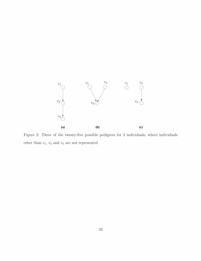
Since each pedigree member has only one set of parents, any possible pedigree G deter-

mines a joint instantiation of the binary variables, I(W → v) in Equation (3) by setting

exactly |V | = n of them to 1 and all the others to 0. For example, if we consider the

pedigree for our toy example in Figure 2(a), we have I({} → v1) = 1 since v1 has no par-

9

ents (i.e. is a founder), I({v1} → v2) = 1 since v2 has one parent v1 in the pedigree and

I({v2} → v3) = 1 to represent that v3 has v2 as its only parent. Analogously, I({} → v1) = 1,

I({v1, v3} → v2) = 1 and I({} → v3) = 1 for Figure 2(b) and I({} → v1) = 1, I({} → v2) = 1

and I({v2} → v3) = 1 for Figure 2(c). This approach allows any pedigree to be mapped to

a set of variables of length n + n(n− 1) + 1

2n(n− 1)(n− 2) each with a value of zero or one.

However, the mapping is not one-to-one as most such sets of variables do not correspond to a

valid pedigree; there is no pedigree that corresponds to all variables being ones, for example.

Noting that I(W → v)(G) only takes the value 1 when W = Pa(v,G), the pedigree

log-likelihood shown in Equation (2) can now be rewritten in terms of these binary variables

as

l(G) = log L(G) =∑

v,W

log τ(v,W ) [I(W → v)(G)] . (4)

The maximum likelihood pedigree reconstruction problem is thus reformulated as a prob-

lem of finding an instantiation of I(W → v) to maximise the quantity shown in Equation (4)

subject to the constraint that this instantiation represents a valid pedigree, G. Since all

the variables are integer-valued and the objective function is linear in these variables, this

satisfies the definition of an integer linear programming problem as long as the constraints

on the I(W → v) can also be expressed as linear equations and inequalities. We show below

that such an expression is indeed possible.

Constraints are required to rule out sets of variable assignments that do not correspond

to a valid pedigree. There are three properties that must be met for a set of assignments

to encode a valid pedigree. First, each individual must have exactly one set of parents.

Second, no individual can ever be his own ancestor. Third, it must be possible to assign sex

consistently to each member of the pedigree. We will now show how each of these properties

can be expressed in the form of linear constraints.

Ensuring one set of parents The most basic constraint, as noted above, is that each in-

dividual, v, has exactly one parent set. This can be expressed concisely by n linear equations

of the form

10

∀v :∑

W

I(W → v) = 1 (5)

For our simple example, these three constraints are as follows:

I({} → v1) + I({v2} → v1) + I({v3} → v1) + I({v2, v3} → v1) = 1

I({} → v2) + I({v1} → v2) + I({v3} → v2) + I({v1, v3} → v2) = 1

I({} → v3) + I({v1} → v3) + I({v2} → v3) + I({v1, v2} → v3) = 1.

To understand why these constraints work, note that for a valid pedigree, exactly one of

the variables in each equation will be equal to 1 (the variable encoding the correct parent

set) and the remaining variables will each be equal to 0. If a variable were to have no parent

set, then the equation for that variable would have its left hand side equal to 0 and hence the

constraint would be violated. Similarly, if a variable were assigned two or more parent sets,

the left hand side would sum to more than 1 and again the constraint would be violated.

Ruling out cycles While an instantiation of the I(W → v) satisfying Equation (5) will

represent a graph where no node can have more than one parent set, these constraints are

not enough to rule out graphs with (directed) cycles i.e. where an individual node can be its

own ancestor or descendant. In our example, setting I({v3} → v1) = 1, I({v1} → v2) = 1

and I({v2} → v3) = 1 would clearly satisfy the constraints in Equation (5) but does not

result in a valid pedigree.

One way to rule out directed cycles, and the approach we use in this paper, is to assign

generation numbers to the individuals. A founder member has generation number zero and

every other individual must have a generation number that is greater than that of each of

its parents. In the absence of any prior knowledge on the maximum generation number, m,

it is possible to use m = n − 1.

For each individual v in the problem, let us introduce a new variable, gen(v), to represent

the generation number of that individual. If gen(v) denotes the generation number assigned

to individual v and u is a parent of v, then we must find assignments to these variables such

11

that gen(v) ≥ gen(u) + 1. Consider the following n(n − 1) constraints:

∀u, v : gen(v) − gen(u) ≥ −m + (m + 1)∑

W :u∈W

I(W → v) (6)

for two distinct individuals labelled u and v. Note that if u is not a parent of v, the

summation∑

W :u∈W I(W → v) on the RHS is 0 and the constraint is vacuously satisfied.

If u is a parent of v, the summation — and hence the entire RHS — is 1 effecting the

desired constraint, gen(v)−gen(u) ≥ 1, on a parent-child relationship. Furthermore, for any

ancestor w of v, it follows that gen(w) < gen(v). A directed cycle necessarily implies that

at least two individuals are their own ancestors leading to an obvious inconsistency. The

constraints in Equation (6) are hence sufficient to rule out such cycles.

The form given in Equation (6) does not correspond to that required for an ILP problem,

but after rearrangement we can write:

∀u, v : (m + 1)∑

W :u∈W

I(W → v) − gen(v) + gen(u) ≤ m (7)

which is in the desired form.

Returning to the example with n = 3 individuals, the 6 new constraints obtained are:

3 [I({v2} → v1) + I({v2, v3} → v1)] − gen(v1) + gen(v2) ≤ 2






Ensuring sex consistency


The constraints given by (5) together with those in (7) are sufficient to ensure that only

variable assignments encoding directed acyclic graphs are allowed. However, not all such

12

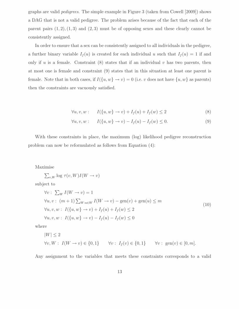
graphs are valid pedigrees. The simple example in Figure 3 (taken from Cowell [2009]) shows

a DAG that is not a valid pedigree. The problem arises because of the fact that each of the

parent pairs (1, 2), (1, 3) and (2, 3) must be of opposing sexes and these clearly cannot be

consistently assigned.

In order to ensure that a sex can be consistently assigned to all individuals in the pedigree,

a further binary variable If (u) is created for each individual u such that If (u) = 1 if and

only if u is a female. Constraint (8) states that if an individual v has two parents, then

at most one is female and constraint (9) states that in this situation at least one parent is

female. Note that in both cases, if I({u,w} → v) = 0 (i.e. v does not have {u,w} as parents)

then the constraints are vacuously satisfied.

∀u, v, w : I({u,w} → v) + If (u) + If (w) ≤ 2 (8)

∀u, v, w : I({u,w} → v) − If (u) − If (w) ≤ 0. (9)

With these constraints in place, the maximum (log) likelihood pedigree reconstruction

problem can now be reformulated as follows from Equation (4):

Maximise∑

v,W log τ(v,W )I(W → v)

subject to

∀v :∑

W I(W → v) = 1

∀u, v : (m + 1)∑

W :u∈W I(W → v) − gen(v) + gen(u) ≤ m

∀u, v, w : I({u,w} → v) + If (u) + If (w) ≤ 2

∀u, v, w : I({u,w} → v) − If (u) − If (w) ≤ 0

where

|W | ≤ 2

∀v,W : I(W → v) ∈ {0, 1} ∀v : If (v) ∈ {0, 1} ∀v : gen(v) ∈ [0,m].

(10)

Any assignment to the variables that meets these constraints corresponds to a valid

13

pedigree. A particular assignment to the variables that also maximises the objective function

is guaranteed to be a maximum likelihood pedigree.

Obviously, for the tiny running example of n = 3 individuals just considered, one could

easily construct and score each of the 25 possible pedigrees and avoid the procedure de-

scribed above. However, that would not scale to larger numbers of individuals. For the ILP

formulation with n individuals, there are only 1

2n3 − 1

2n2 + 3n variables and n3 − 2n2 + 2n

constraints so, in principle, the method should extend to reasonably large problems.

Note that, for any given situation, the number of variables and constraints to be consid-

ered may in fact be lower. We consider a genetic model in which there is no mutation; this

means that τ(v,W ) = 0 for many combinations of parent set W and child u. A valid pedigree

will hence not contain such relationships and the value of the corresponding I(W → v) has

to be 0. Once these variables are fixed at 0, some of the constraints featuring these variables

may be provably satisfied by any valid assignment of values to the remaining variables. Such

redundant constraints can then be removed.

2.3 Additions and improvements to the ILP formulation

Having formulated the problem of finding the most likely pedigree as an ILP problem, we

introduce some slight modifications that improve the solving performance and allow for the

k most likely pedigrees to be found.

At least one founder Preliminary experiments revealed that explicitly adding the implied

constraint that there has to be at least one pedigree founder greatly increases the performance

of the algorithm. This is given as

∑

v

I({} → v) ≥ 1. (11)

This is always trivially true since pedigrees are acyclic and so a maximum likelihood

pedigree will still be returned.

Finding the kth most likely pedigree As already noted, finding a single maximum

likelihood reconstruction does not take account of model uncertainty, and for this reason,

14

we wish to find multiple high likelihood pedigrees. Specifically, we want to find the k most

likely pedigrees, for some arbitrary value k. This can be done by repeatedly solving the ILP

problem given in (10), adding one additional constraint each time to prevent a previously

found solution from being returned again. In this way, repeated solutions of the problem

yield valid pedigrees in order of descending likelihood.

The additional constraint added each time is as follows:

∀ W, v s.t. I(W → v)(G) = 1 :∑

W,v

I(W → v) < n (12)

where G is the previously found pedigree. The constraint simply states that at least one

parent set in the new pedigree has to differ from the previous one. For the kth most likely

pedigree, there will be k−1 such constraints, one for each of the previously found pedigrees.

2.4 Marker data and pedigree structures

In order to assess how well the method performs, the results reported in Section 3 are based

on simulated datasets about which there is no uncertainty. To generate each dataset, genetic

profiles were created for each individual of a given pedigree based on a given distribution of

population allele frequencies under the assumptions stated in Section 2.1. We simulated 100

datasets for each combination of pedigree structure and set of allele frequencies considered.

Allele Frequencies We simulated data from two sets of allele frequencies, both based on a

typical forensic set of microsatellite markers. We used the original (not rounded) Caucasian

allele frequencies for the 15 autosomal short tandem repeat loci (the 13 CODIS core loci plus

D19S433 and D2S1338) corresponding to Table 1 of Butler et al. [2003] as an example of

a realistic distribution. These allele frequencies were previously used for the same purpose

in Cowell [2009]. For our second set of frequencies, we considered the same 15 marker set

but assigned equal probabilities to the listed alleles for each marker. This is what we will

refer to as our ‘uniform frequency distribution’. In both cases, we thus have 15 markers with

allele numbers ranging between 7 and 15.

15

Pedigrees




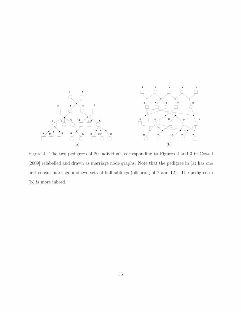
Several pedigree structures are considered. For direct comparison with the results re-

ported in Cowell [2009], we used the two small pedigrees of 20 individuals considered in

that paper and reproduced in Figure 4. As an example of a larger structure, we took the

59-member pedigree of Almudevar [2003], reproduced here in Figure 5, as a reasonable repre-

sentation of the complexity to be expected in a typical human pedigree. In order to consider

a pedigree complexity effect, we also considered the cyclic half-sib, cyclic first cousin and

quadruple second cousin regular mating structures of Wright [1921], each with 64 individuals

i.e. 7 generations descended from 8 founders. The half-sib structure is the most inbred of

the three. However, although there are no matings between close relatives in the quadru-

ple second cousin pedigree shown in Figure 6, it requires only four generations before all

individuals are related to all eight founders.

3 Results

Initial reported results using integer linear programming for maximum likelihood pedigree

reconstruction are encouraging [Cussens, 2010]. Here, we will perform a more detailed ex-

ploration where we aim to assess how well our algorithm performs on a range of pedigrees.

We will consider the time needed by this approach to find the most likely pedigree and also

the time needed to find the kth most likely pedigree.

Further to this, we examine the suitability of any approach which searches for maximum

likelihood pedigrees by examining the similarity between the real pedigree and the maximum

likelihood one. This is developed into considering the distribution of likelihood over the

k most likely pedigrees. Finally, we compare our approach to those presented by Cowell

[2009], Riester et al. [2009] and Almudevar [2003].

16

All reported results were produced on a normal desktop computer (2.8GHz quad-core

running Windows 7) with the Gurobi ILP solver, for which a free academic licence is available.

3.1 Solution Times

For the four larger pedigrees (the 59 member one shown in Figure 5 and the three regular

mating structures studied), we first considered the time taken to find a most likely pedigree

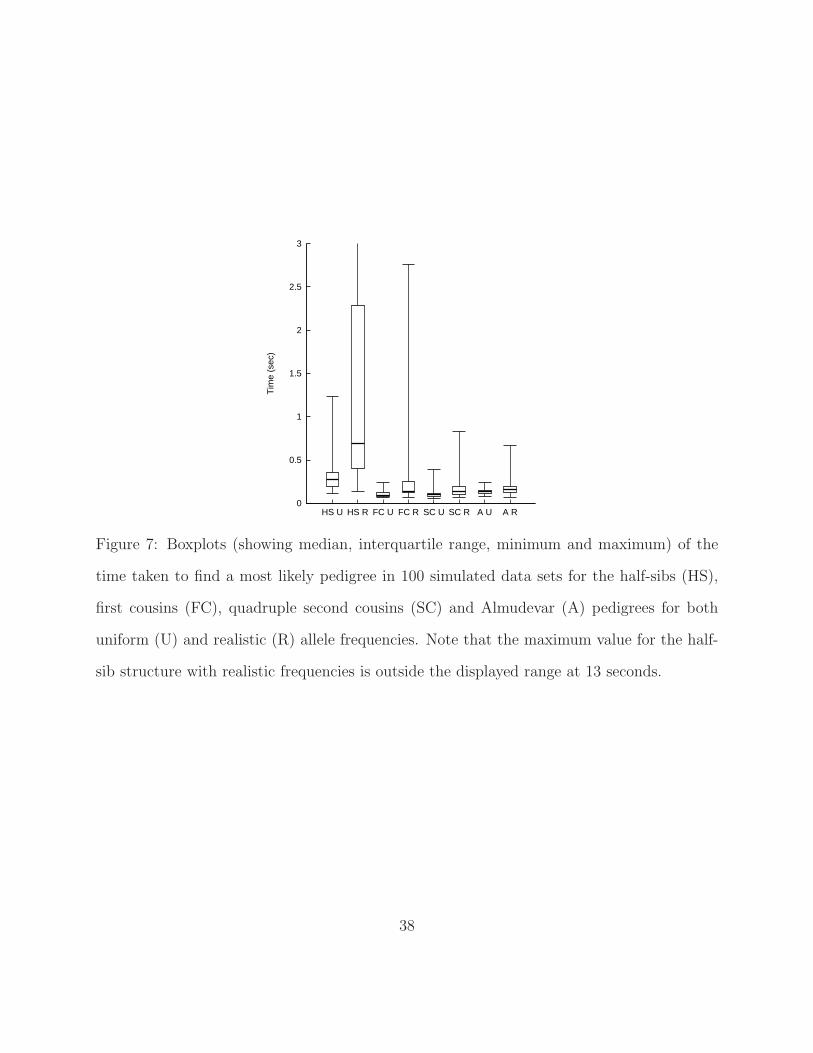
for the 100 data sets simulated from both sets of allele frequencies. Side by side boxplots of

these time distributions are shown in Figure 7.


The results show that a maximum likelihood solution was usually found very quickly with

the most extreme case taking about 1.3 seconds when uniform allele frequencies were used.

Note that, despite the fact that we have differing numbers of alleles at each locus, uniform

allele frequencies clearly make the reconstruction problem easier. Typical solving times were

always slower and much more variable with realistic frequencies on all four pedigrees. The

cyclic half-sib pedigree proved to be the most challenging structure for the algorithm, in

terms of solving time, with an extreme value of 13 seconds when marker data were simulated

from the realistic allele frequency distribution. The pedigree in Figure 5 and the quadruple

second cousin structure in Figure 6 were the easiest with the maximum likelihood solution

always found within a second.


As noted earlier, a single maximum likelihood reconstruction is not always particularly

useful so we now consider the 100 most likely pedigrees. Figure 8 shows the median times

taken between finding the (k − 1)th and the kth most likely pedigree for all four structures

and both sets of allele frequencies. The overall pattern is that the maximum likelihood

pedigree (i.e. the first of the 100 pedigrees) is found most quickly and solving times tend to

increase for each additional pedigree sought. Solving times are slower for the realistic allele

frequencies than for the uniform ones and are more variable for the pedigree of Figure 5 and

the half-sib structure than for the other two regular structures. The cyclic half-sib structure

is markedly more difficult to solve with increasing number of pedigrees found.

17

3.2 Accuracy of the reconstructed pedigree

Assessing the value of a particular reconstruction depends to some extent on what it is

required for. Often, as would be the case for demographic research or ecological studies that

aim to design a breeding program, it is more important that the estimated pedigree reflect

general characteristics of the true structure, such as correct distribution of sibship sizes,

correct levels of multiple marriages and overall connectedness of the sampled individuals,

rather than be accurate in every detail [Thompson, 1986]. There are many such criteria

that may be important and these will differ between applications. We therefore focus on

a general property for assessing the quality of the reconstruction, while noting that this

may not be the best criterion in any given situation. Comparing the number of erroneous

parent-offspring links (or incorrect graph edges) is an obvious statistic and is commonly

used in BN learning. However, it should be noted that although a maximum likelihood

pedigree is often a reasonable approximation to the true pedigree, whether it is or not has

no bearing on the speed and exactness of a method for finding it. Our goal is to find high

likelihood pedigrees quickly so it could be argued that error rates such as the mean number

of parental misspecifications are not the appropriate statistics for evaluating the success of

a likelihood approach. Nevertheless, they can be useful — particularly when several high

likelihood pedigrees are considered.

[Table 1 about here.]

Table 1 shows the sample distribution of incorrect parent-offspring links among the 100

maximum likelihood pedigrees for each of the 8 combinations of allele frequency and pedigree

structure. Specifically, we define a link to be incorrect if it is either missing or incorrectly

attributed. The maximum number of such errors is twice the number of individuals. As can

be seen, the maximum likelihood pedigrees had considerably fewer incorrect links when the

data were simulated under uniform allele frequencies than for the case with realistic frequen-

cies. The reconstruction of the pedigree in Figure 5, which is a more realistic representation

of a human pedigree structure, was most often correct or close to correct. Quadruple second

cousins were the most accurate of the regular mating systems we considered by this mea-

sure. The cyclic half-sib maximum likelihood reconstruction was the least likely to be the

18

true structure with as many as 8 misspecified parent-offspring links even for the uniform

allele frequency scenario. Accuracy of reconstruction appears to deteriorate with increasing

levels of inter-relatedness. From the form of the optimisation function in (4), the algorithm

is choosing the ‘best’ parentage for each individual. The more inter-related the individuals,

the more genetically consistent choices there are for parent pairs or triplets. This is consis-

tent with the observation in Thompson [1986] that high exclusion probabilities for incorrect

parents are required in order to obtain an accurate reconstruction.

[Table 2 about here.]

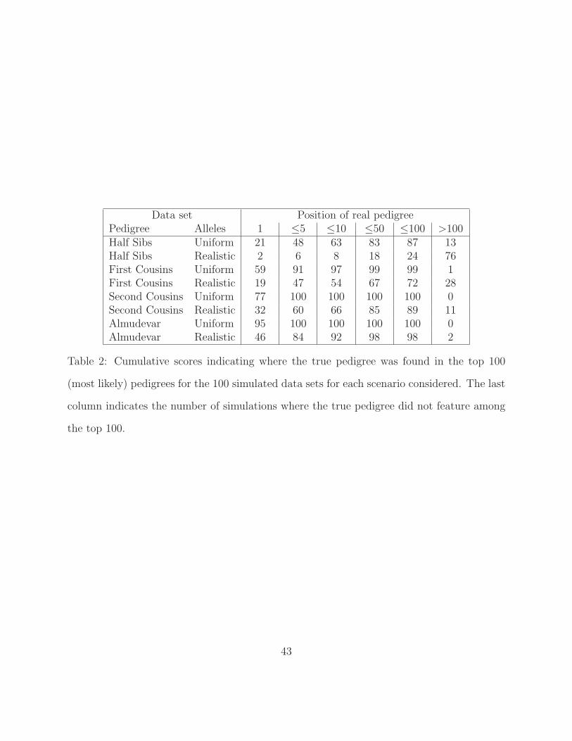
It is reasonable to expect that while the true pedigree may not always have maximum

likelihood, the inferred relationships should include many of the true parent-child links and

so the true pedigree should often feature among the most likely ones. Table 2 shows where

the true pedigree was found among the 100 most likely pedigrees for all 100 simulated data

sets for each scenario considered. For the uniform allele frequency distribution, the maximum

likelihood pedigree was actually the true pedigree 95% of the time for the pedigree of Figure 5.

The story was quite different for the realistic frequencies where the true pedigree did not

appear in the top 100 reconstructions for 2 of the runs. There was a similar trend for the

regular mating structures with the cyclic half-sib pedigree being the hardest to get right: the

true structure was the first one found in 2 runs but 76 had failed to find it among the first

100 for the realistic allele frequency distribution. These results highlight the importance

of being able to generate multiple high probability pedigrees rather than rely on a single

reconstruction.

3.3 Distribution of likelihoods


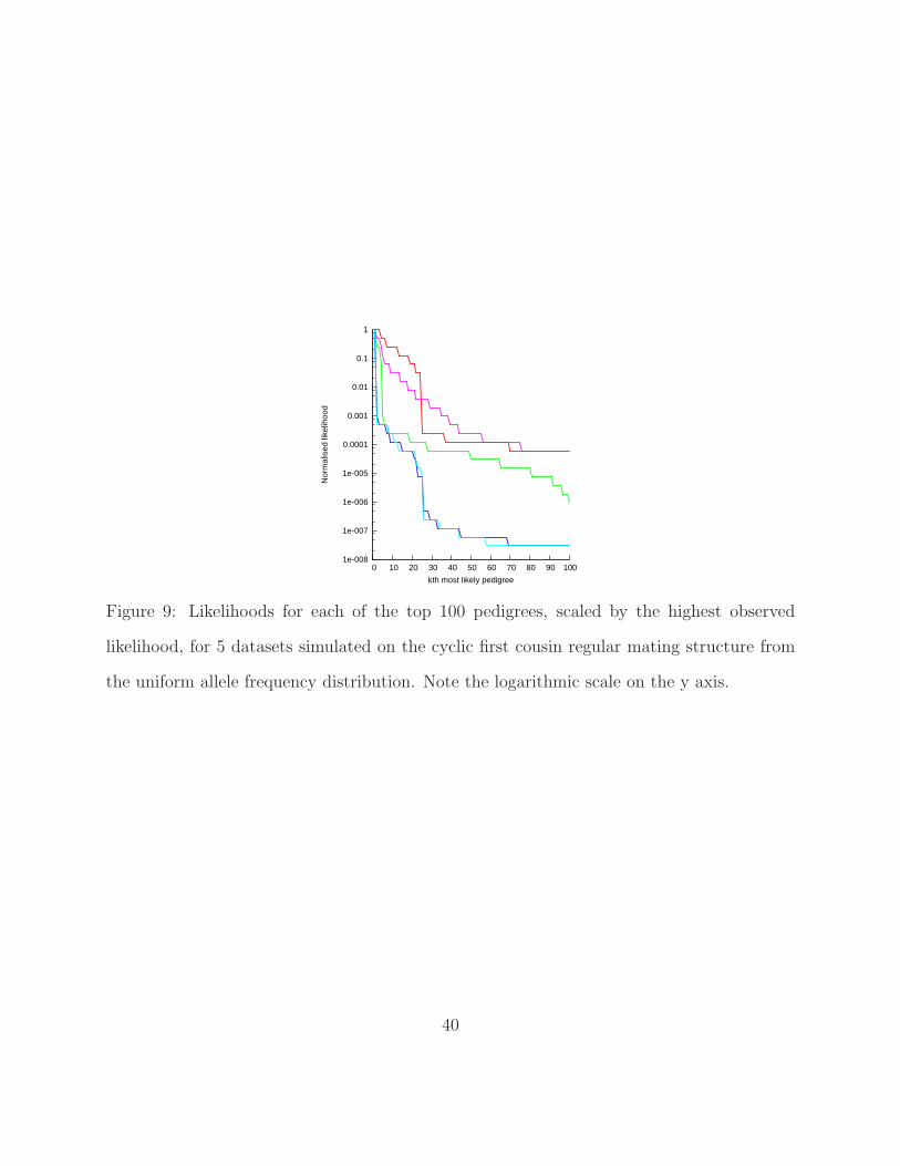
In order to get an idea of what the search space of pedigree likelihoods looks like, we

investigated the relative distribution of the likelihoods of the top 100 pedigrees. Because

likelihoods vary considerably with different combinations of simulated data and pedigree

structure, we divided the likelihood of the kth most likely pedigree in each of the 100 runs

19

by the value of the likelihood for the first pedigree found in that run. Examples of how

variable these are for some particular data sets are given in Figure 9 for the first cousin

64-member pedigree. As can be seen, the likelihoods tend to drop sharply soon after the top

pedigree is found, plateau out and then drop again several times to a tail of low likelihood

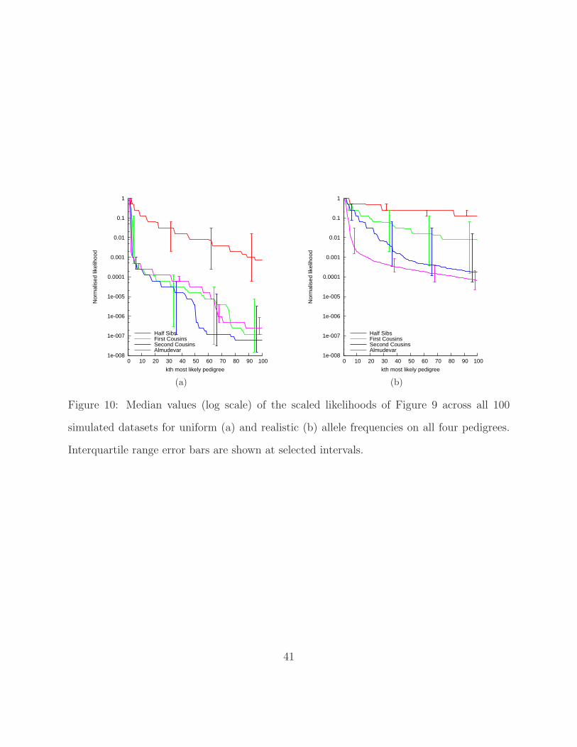
pedigrees. Median values across the 100 simulated datasets with interquartile range error

bars at selected intervals are displayed in Figure 10 for all four pedigree structures using the

uniform (a) and realistic (b) allele frequencies. The y-axis has been plotted on a log scale to

stretch out the lower values because of the sharp drop in likelihood at the outset.


Likelihoods drop more quickly for the uniform allele frequencies, again reflecting the fact

that maximum likelihood pedigree reconstruction is easier with uniform frequencies than

with more realistic ones. For our set of realistic allele frequencies, the likelihoods of the

reconstructed cyclic half-sib pedigrees are not surprisingly the slowest to drop and are by far

the least variable indicating the difficulty of the optimisation problem.

3.4 Comparison with other approaches

There are three other notable approaches to maximum likelihood pedigree reconstruction [Al-

mudevar, 2003; Cowell, 2009; Riester et al., 2009] against which we will now compare our

approach.

The method described by Almudevar [2003] relies on simulated annealing to search for a

maximum likelihood pedigree. However, any method such as this that uses a heuristic search

cannot be guaranteed to find the actual maximum likelihood pedigree. The results shown in

Figure 10 illustrate the particular problem with this in the context of pedigree reconstruction;

the most likely pedigree can be orders of magnitude more likely than the next few most likely.

Methods that do not necessarily find the most likely pedigree may instead find pedigrees

significantly less likely than the best. Calculation times reported in Almudevar [2003] are

of the order of minutes, compared to sub-second times for reconstructing the same pedigree

using our method. It should also be noted that the evaluation presented in Almudevar [2003]

20

is conducted under the assumption of uniform allele frequency. Our results show that this

makes the pedigree reconstruction problem easier than it would be using realistic frequencies.

As for our method, the dynamic programming approach of Cowell [2009] guarantees

a maximum likelihood pedigree. However, that approach is restricted to small pedigrees

due to storage requirements (i.e. up to about 30 individuals). For direct comparison, the

dynamic programming approach to maximum likelihood pedigree reconstruction of Cowell

[2009] and the ILP algorithm of Section 2.2 were both run on 100 simulated data sets for

both sets of allele frequencies on the two pedigrees in Figure 4. Both algorithms were quick

(less that 1 second) to find a single maximum likelihood pedigree. Solving times for the

dynamic programming method were all consistently between 0.45 to 0.5 seconds while the

ILP approach was noticeably faster with 90% of the runs succeeding in less than 0.25 seconds.

The dynamic programming approach occasionally found a sex-inconsistent pedigree but this

never happened with the ILP algorithm as the search was constrained to rule out such

structures. Solving time was a little longer for the more inbred pedigree of Figure 4(b) and

this became more apparent when many high probability pedigrees were sought with the ILP

algorithm. In terms of the number of correctly inferred parent-offspring relationships, the

maximum likelihood pedigree was always very close to the true pedigree structure with ≤ 3

different links 95% of the time. The true pedigree almost always featured among the 10 most

likely pedigrees when these could be found and, not unexpectedly, the likelihood distribution

dropped off dramatically after the top 10 pedigrees, or so. For cyclic half-sib structures of

100 individuals, we found that the algorithm took considerably longer to find a maximum

likelihood pedigree. For realistic allele frequencies, 75% of the runs found a solution in less

than 100 seconds but some took as long as 4 hours. This is not too surprising, given that this

was by far the hardest structure we considered, and we would expect much better results for

less complex structures.

Riester et al. [2009] present a software tool for pedigree reconstruction. At the core of the

tool, a solution is found using either the method of Almudevar [2003] or that of Cowell [2009].

Hence, the tool suffers from the disadvantages discussed above: either the pedigree cannot

be guaranteed to be the most likely or the number of individuals that can be considered is

seriously limited. However, it does incorporate several features that we have not addressed.

21

The likelihoods of parentage triples are modified in a principled way to admit the possibility

of genotyping errors and to compensate for a finite number of mating individuals in the

population. These likelihoods are also modified during the search process based on the

current beliefs about population allele frequencies, rather than assuming such frequencies

are known accurately a priori. The tool also allows for potential missing data for some

individuals by repeatedly estimating values for such data during the search process using

Gibbs sampling.

To the best of our knowledge, our ILP algorithm is the only approach to maximum

likelihood pedigree reconstruction that can deliver the k most likely pedigrees and can thus

address the issue of model uncertainty.

4 Discussion

4.1 Extensions to more complex problems

The method we have presented here performs well under the assumptions of a complete sam-

ple, independently segregating genetic markers and Hardy-Weinberg proportions for founder

genotypes. In particular, when complete marker data are observed for all individuals, an

offspring genotype is independent of all non-descendant genotypes conditional on the geno-

types of its parents. This is generally known as the (directed local) Markov property for

Bayesian networks and results in the decomposition of the (log) likelihood function in Equa-

tions (1) and (4) which is the core of our ILP formulation. As noted in Lauritzen and Sheehan

[2003], Mendelian inheritance of offspring genotypes from parental types is also implicit in

this decomposition. Contrary to the statement in Cowell [2009], the desired decomposition

breaks down when markers are linked and siblings are no longer conditionally independent

given their parents. This can be easily seen for the case of two linked marker loci with a

recombination fraction r and alleles A1, A2, A3 and B1, B2, B3, respectively. Consider two

offspring from a doubly heterozygous (A1A2, B1B2) and doubly homozygous (A3A3, B3B3)

mating where parental phase is unknown. We are interested in the probability of the second

offspring, I2, having genotype (A1A3, B1B3). If the first offspring, I1 is also (A1A3, B1B3),

22

P (I2 = (A1A3, B1B3)|I1 = (A1A3, B1B3)) =1

4(1 − r)2 +

1

4r2

i.e. both offspring inherited both alleles from the same chromosome (no recombination) or

they both inherited them from different chromosomes. If I1 is (A1A3, B2B3), we have that

P (I2 = (A1A3, B1B3)|I1 = (A1A3, B2B3)) =1

2r(1 − r)

i.e. there was a recombination for one offspring and not for the other. In order for the Markov

property to hold, both these probabilities should be equal. This is clearly true only when

r = 1

2i.e. when the loci are unlinked.

Complete data will generally not be available when constructing pedigrees for linkage

analysis or for identifying distant relatives for homozygosity mapping from human population

studies. The same is true for wildlife management and forensic science applications. In these

cases, unobserved individuals that form ‘missing links’ between the individuals of interest

have to be accounted for and the likelihood in Equation (1) has to be modified by summing

over all possible combinations of genotypes on the unobserved individuals [Thompson, 2000].

The more unobserved individuals, the larger the sum and the more difficult the likelihood

computation. In order to extend our approach to include individuals with wholly or partially

missing marker data, the missing information could be represented using additional variables

so that the log-likelihood remains linear. The number of additional variables required should

be modest if there is no linkage and the approach should be feasible given the observed

efficiency of the algorithm. An alternative method is suggested by Riester et al. [2009]

whereby missing data are estimated during the reconstruction using Gibbs sampling.

Existing likelihood approaches to pedigree construction are all based on independently

segregating genetic markers. Likelihood calculations are hence simplified, as was the case

in this paper, since only one marker has to be considered at any one time. There are some

relationships, however, that have the same likelihood and are hence indistinguishable for

any number of unlinked markers, but are distinguishable with linked markers [Thompson,

1975; Egeland and Sheehan, 2008]. Given the ever increasing availability of dense sets of

SNPs from genetic association studies, reconstruction algorithms should aim to make use of

23

linked markers. Correlated markers naturally lead to a reduction in discriminatory power

when compared with (the same number of) unlinked markers so it is to be expected that

many more markers will be required. Preliminary work for distinguishing between particular

alternatives for pairwise relationships has shown that huge numbers of markers, as are now

readily available for genetic association studies, can be used to distinguish between quite

distant relationships [Skare et al., 2009]. In order to adapt our method for handling linked

markers, we could adopt a similar strategy to that described above for missing data by repre-

senting the unknown phase information with additional variables. This restores the desired

decomposition of the likelihood function and the optimisation procedure now returns a most

probable combination of pedigree structure and haplotypes. Note that the observed (un-

ordered) marker data put tight constraints on the possible haplotypes and these constraints

are easy to express in the ILP framework. It is no surprise that ILP has been successfully

used for inferring haplotypes in the case where the true pedigree is known [Brown and Har-

rower, 2006]. Likelihood calculations will be much more intensive for linked markers and we

may realistically need to consider approximations.

Finally, in addition to genetic marker data, prior population demographic information on

breeding patterns, average numbers of offspring and cultural prejudices, for example, as well

as specific knowledge about particular relationships may often be available in practice. It is

important to include such information when reconstructing pedigrees since structures that

fit the marker data the best may be unreasonable in other respects, such as by representing

improbably high levels of interrelatedness, for the population in question [Egeland et al.,

2000]. More importantly, a formal Bayesian approach permits a principled way of quantifying

model uncertainty using Bayesian model averaging [Kass and Raftery, 1995; Hoeting et al.,

1999].

Many existing approaches [Hadfield et al., 2006; Neff et al., 2001; Riester et al., 2009;

Thompson, 1976a; Thompson and Meagher, 1987] do incorporate some prior information,

but often in an informal way and at an interim stage of the reconstruction, for example

when the likelihood approach is favouring what is clearly an undesirable structure [Sheehan

and Egeland, 2007]. If sensible priors could be assigned to pedigrees [Egeland et al., 2000;

Sheehan and Egeland, 2007], the likelihood of any candidate pedigree L(G), based on the

24

observed marker data, can be combined with a prior probability π(G) to derive the posterior

probability p(G | data) ∝ π(G)L(G) using Bayes’ theorem. The pedigree reconstruction prob-

lem then reduces to a search for a pedigree with maximal posterior probability, often called

MAP estimation. This is equivalent to likelihood estimation in the case of a uniform prior

distribution over all possible pedigrees.

Extending our approach to deal with priors should be quite simple. If the prior encodes

‘hard’ information (e.g. an individual is female, or a particular individual is the parent of

another), this can be added to the ILP formulation as additional constraints. If the prior

encodes ‘soft’ information (e.g. a probability distribution over sibship sizes), it can be shown

that this can be accurately incorporated into the problem through the addition of extra log

prior terms to the objective function, provided that the prior can be encoded as a linear

function.

4.2 Conclusions

Family relationships, and hence pedigrees, are central to all gene mapping studies [Day-

Williams et al., 2011]. Establishing pedigree information through interviews and historical

records is time consuming and so it is appealing to be able to reconstruct pedigrees from

genetic marker data using available large population studies, especially since such studies

have a reasonable chance of representing extended pedigree information which is otherwise

difficult to obtain [Browning and Browning, 2010]. The ILP approach to pedigree reconstruc-

tion that we have presented in this paper has been shown to out-perform other approaches

in the standard setting where all individuals are observed, segregation is Mendelian, markers

are independent and founder genotypes are in Hardy-Weinberg equilibrium. It also extends

to quite large pedigrees, guarantees a maximum likelihood solution and can deal with un-

certainty in the reconstruction by providing the k most likely pedigrees. Most importantly,

we have a framework that seems more amenable to adaptation to harder, and hence more

interesting, reconstruction problems. Our algorithm usually finds a maximum likelihood

pedigree efficiently but is sensitive to the allele frequency distribution and the complexity of

the pedigree structure. We would warn that the use of uniform allele frequencies, as com-

monly arises in simulation studies, can be misleading as they make the problem deceptively

25

easier.

It can be argued that likelihood approaches are not necessarily the most useful for pedi-

gree estimation, especially when general features or specific sections of the pedigree are of

more interest that the overall structure. Comparison of estimates is much less straightfor-

ward in these situations, although realising an appropriate one is generally simpler. For small

populations, multidimensional scaling of pairwise kinship coefficients has been suggested as

one way of representing general population structure [Thompson, 1986]. Where the overall

structure is of interest, however, we have verified that maximising the likelihood is a good

approach. Unless the structure is extremly complex, the maximum likelihood pedigree is

typically quite similar to the true structure with regard to the number of parent-offspring

links that are correctly assigned and usually features quite early in the list of most likely

pedigrees. We agree with the comment in Thompson [1986] that a single maximum likeli-

hood estimate may not be particularly helpful but useful inferences should be possible from

several high probability pedigrees. For example, reasonable probability estimates of particu-

lar pedigree features can be acquired from the proportion of high probability structures that

contain them.

Pedigree reconstruction has also been proposed using a two-step approach that involves

estimation of pairwise kinship coefficients followed by clustering of individuals into pedigrees

using graph learning methods [Cowell and Mostad, 2003; Day-Williams et al., 2011]. This ap-

proach is also sensitive to allele frequencies and the choice of cut-off value used to determine

the graph edges. For quantitative trait locus (QTL) linkage analysis, pedigree information is

only incorporated via local and global pairwise kinship coefficients so estimating these quan-

tities from marker data using dynamic programming and a method of moments approach,

respectively, can obviate the need for standard pedigrees in such analyses [Day-Williams

et al., 2011]. In fact, it has also been noted by Choi et al. [2009] that estimated kinship

coefficients can often be more accurate than pedigree-based quantities because they exploit

the observed sharing of genes between two individuals rather than the expected sharing im-

plied by the pedigree structure. The ILP approach presented here also uses the observed

sharing but has the advantage of considering all related individuals jointly in the likelihood

calculation. We would thus expect it to have an advantage over approaches based on pair-

26

wise estimates and, indeed, in the simple standard scenario we considered here, we do not

think that one could do much better. However, we need to extend the method to deal with

unobserved individuals and linked markers before a sensible comparison can be made. Also,

when extended pedigrees are of interest, genotyping error and/or mutation rates should also

be included. These are much harder reconstruction problems but ILP would seem to provide

the right framework in which to address them.

Acknowledgements

The authors would like to thank Robert Cowell for giving access to his code.

The authors acknowledge support from the Medical Research Council (Project Grant G1002312),

the Leverhulme Trust (Research Fellowship RF/9/RFG/2009/0062) and the BioSHaRE-EU

project (HEALTH-F4-2010-261433) funded by the European Commission under the Seventh

Framework Program (FP7/2007-2013).

References

Almudevar, A. (2003). A simulated annealing algorithm for maximum likelihood pedigree

reconstruction. Theoretical Population Biology, 63:63–75.

Almudevar, A. (2007). A graphical approach to relatedness inference. Theoretical Population

Biology, 71:213–229.

Blouin, M. S. (2003). DNA-based methods for pedigree reconstruction and kinship analysis

in natural populations. Trends in Ecology and Evolution, 18:503–511.

Brown, D. and Harrower, I. (2006). Integer programming approaches to haplotype inference

by pure parsimony. IEEE/ACM Transactions in Computational Biology and Bioinformat-

ics, 3(2):141–154.

Browning, S. R. and Browning, B. L. (2010). High-resolution detection of identity by descent

in unrelated individuals. American Journal of Human Genetics, 86:526–539.

27

Butler, J. M., Schoske, R., Vallone, P. M., Redman, J. W., and Kline, M. C. (2003). Allele

frequencies for 15 autosomal STR loci on U.S. Caucasian, African American, and Hispanic

populations. Journal of Forensic Sciences, 48(4).

Cannings, C. and Thompson, E. A. (1981). Genealogical and Genetic Structure. Cambridge

University Press.

Cannings, C., Thompson, E. A., and Skolnick, M. H. (1978). Probability functions on

complex pedigrees. Advances in Applied Probability, 10:26–61.

Choi, Y., Wijsman, E. M., and Weir, B. S. (2009). Case-control testing in the presence of

unknown relaionships. Genetic Epidemiology, 33:668–678.

Cowell, R. G. (2009). Efficient maximum likelihood pedigree reconstruction. Theoretical

Population Biology, 76(4):285–291.

Cowell, R. G. and Mostad, P. (2003). A clustering algorithm using DNA marker information

for sub-pedigee reconstruction. Journal of Forensic Sciences, 48:1239–1248.

Cussens, J. (2010). Maximum likelihood pedigree reconstruction using integer programming.

In Workshop on Constraint Based Methods for Bioinformatics (WCB-10), Edinburgh.

Day-Williams, A. G., Blangero, J., Dyer, T. D., Lange, K., and Sobel, E. M. (2011). Linkage

analysis without defined pedigrees. Genetic Epidemiology, 35(5):360–370.

Egeland, T., Mostad, P. F., Mevag, B., and Stenersen, M. (2000). Beyond traditional

paternity and identification cases: selecting the most probable pedigree. Forensic Science

International, 110:47–59.

Egeland, T. and Sheehan, N. (2008). On identification problems requiring linked markers.

Forensic Science International: Genetics, 2:219–225.

Genin, E. and Clerget-Darpoux, F. (1996). Consanguinity and the sib-pair method: an

approach using identity by descent between and within individuals. American Journal of

Human Genetics, 59:1149–1162.

28

Hadfield, J. D., Richardson, D. S., and Burke, T. (2006). Towards unbiased parentage

assignment: combining, genetic, behavioural and spatial data in a Bayesian framework.

Molecular Ecology, 15:3715–3730.

Hoeting, J. A., Madigan, D., Raftery, A. E., and Volinsky, C. T. (1999). Bayesian model

averaging: a tutorial. Statistical Science, 14(4):382–401.

Jones, A. G. and Ardren, W. R. (2003). Methods of parentage analysis in natural populations.

Molecular Ecology, 12:2511–2522.

Karp, R. (1972). Reducibility among combinatorial problems. In Miller, R. and Thatcher,

J., editors, Complexity of Computer Computations, pages 85–103. Plenum Press.

Kass, R. E. and Raftery, A. E. (1995). Bayes factors. Journal of the American Statistical

Association, 90(430):773–795.

Lange, K. and Elston, R. C. (1975). Extensions to pedigree analysis. I. Likelihood calculations

for simple and complex pedigrees. Human Heredity, 25:95–105.

Lauritzen, S. L. (1996). Graphical Models. Clarendon Press, Oxford, United Kingdom.

Lauritzen, S. L. and Sheehan, N. (2003). Graphical models for genetic analyses. Statistical

Science, 18:489–514.

Leutenegger, A. L., Prum, B., Genin, E., Verny, C., Lemainque, A., Clerget-Darpoux, F.,

and Thompson, E. A. (2003). Estimation of the inbreeding coefficient through use of

genomic data. American Journal of Human Genetics, 73:516–523.

McPeek, M. S. and Sun, L. (2000). Statistical test for detection of misspecified relationships

by use of genome-screen data. American Journal of Human Genetics, 66:1076–1094.

Meagher, T. R. and Thompson, E. A. (1987). Analysis of parentage for naturally established

seedlings of Chamaelirium luteum (liliaceae). Ecology, 68:803–812.

Neff, B. D., Repka, J., and Gross, M. R. (2001). A Bayesian framework for parentage

analysis: the value of genetic and other biological data. Theoretical Population Biology,

59:315–331.

29

Newman, D. L., Abney, M., McPeek, M. S., Ober, C., and Cox, N. J. (2001). The importance

of genealogy in determining genetic associations with complex traits. American Journal

of Human Genetics, 69:1146–1148.

Olaisen, B., Stenersen, M., and Mevag, B. (1997). Identification by DNA analysis of the

victims of the August 1996 Spitsbergen civil aircraft disaster. Nature Genetics, 15:402–405.

Powell, J. E., Visscher, P. M., and Goddard, M. E. (2010). Reconciling the analysis of IBD

and IBS in complex trait studies. Nature Reviews:Genetics, 11:800–805.

Riester, M., Stadler, P. F., and Klemm, K. (2009). FRANz: reconstruction of wild multi-

generation pedigrees. Bioinformatics, 25:2134–2139.

Sanchez, M., Givry, S. d., and Schiex, T. (2008). Mendelian error detection in complex

pedigrees using weighted constraint satisfaction techniques. Constraints, 13:130–154.

Sheehan, N. A. and Egeland, T. (2007). Structured incorporation of prior information in

relationship identification problems. Annals of Human Genetics, 71:501–518.

Sheehan, N. A. and Egeland, T. (2008). Adjusting for founder relatedness in a linkage

analysis using prior information. Human Heredity, 65(4):221–231.

Sieberts, S. K., Wijsman, E. M., and Thompson, E. A. (2002). Relationship inference from

trios of individuals in the presence of typing error. American Journal of Human Genetics,

70:170–180.

Skare, O., Sheehan, N., and Egeland, T. (2009). Identification of distant family relationships.

Bioinformatics, 25:2376–2382.

Stankovich, J., Bahlo, M., Rubio, J. P., Wilkinson, C. R., Thomson, R., Banks, A., Ring, M.,

Foote, S. J., and Speed, T. P. (2005). Identifying nineteenth century links from genotypes.


Thomas, A. (1985). Data structures, methods of approximation and optimal computation for

pedigree analysis. PhD thesis, Cambridge University.

30

Thompson, E. A. (1975). The estimation of pairwise relationships. Annals of Human Ge-

netics, 39:173–188.

Thompson, E. A. (1976a). Inference of genealogical structure. Social Science Information,

15:477–526.

Thompson, E. A. (1976b). A paradox of genealogical inference. Advances in Applied Proba-

bility, 8:648–650.

Thompson, E. A. (1986). Pedigree Analysis in Human Genetics. The Johns Hopkins Uni-

versity Press, Baltimore.

Thompson, E. A. (2000). Statistical Inference from Genetic Data on Pedigrees, volume 6 of

NSF-CBMS Regional Conference Series in Probability and Statistics. Institute of Mathe-

matical Statistics and the American Statistical Association, Beachwood, Ohio, USA.

Thompson, E. A. (2008a). Analysis of data on related individuals through inference of iden-

tity by descent. Technical Report 539, Department of Statistics, University of Washington.

Thompson, E. A. (2008b). The IBD process along four chromosomes. Theoretical Population

Biology, 73:369–373.

Thompson, E. A. and Meagher, T. R. (1987). Parent and sib likelihoods in genealogy

reconstruction. Biometrics, 43:585–600.

Thornton, T. and McPeek, M. S. (2010). ROADTRIPS: Case-control association testing with

partially or completely unknown population and pedigree structure. American Journal of


Wolsey, L. A. (1998). Integer Programming. Wiley-Interscience Series in Discrete Mathe-

matics and Optimization. Wiley.

Wright, S. (1921). Systems of mating. Genetics, 6:111–178.

31

(a) (b) (c)

Figure 1: A simple pedigree in standard form (a); with corresponding representations as a

directed acyclic graph (b); and marriage node graph (c).

32

(a) (b) (c)

v1v1v1

v2

v2 v2

v3

v3

v3

Figure 2: Three of the twenty-five possible pedigrees for 3 individuals, where individuals

other than v1, v2 and v3 are not represented

33

1 2 3

4 5 6

Figure 3: A simple DAG where no node has more than two parent nodes but which is not

a pedigree as sex cannot be consistently assigned. Since 2 and 3 have a child together, they

must be of opposite sex. However as they each have a child with 1, they must have the same

sex. It is clearly impossible to assign sexes that meet these contradictory constraints.

34

1 2

2 4 5 6

16

7 8 9 10 1211

201918171513 14

(a)

1 2 3 4 5

6 7 8 9 19

11 12 13 14 15

16 17 18 19 20

(b)

Figure 4: The two pedigrees of 20 individuals corresponding to Figures 2 and 3 in Cowell

[2009] relabelled and drawn as marriage node graphs. Note that the pedigree in (a) has one

first cousin marriage and two sets of half-siblings (offspring of 7 and 12). The pedigree in

(b) is more inbred.

35

1 6 8 9

12 13 14 15 16 17 18 21 22 23 24

25 26 30

35 36 37 38 40 42 43 44 47

48 50 51 53 54 55 56 57 59

2 73 4 5

10 11 19 20

27 28 29 31 32 33 34

39 41 45 46

49 52 58

Figure 5: A 59-member pedigree featuring some first cousin marriages and half-siblings taken

from Almudevar [2003].

36

1 2 3 4 5 6 7 8

71 72 73 74 75 76 77 78

61 62 63 64 65 66 67 68

51 52 53 54 55 56 57 58

4847464544434241

31 32 33 34 35 36 37 38

2827262524232221

11 12 13 14 15 16 17 18

Figure 6: A 64-member pedigree constructed as a quadruple second cousin regular mating

structure as described in Wright [1921].

37

0

0.5

1

1.5

2

2.5

3

HS U HS R FC U FC R SC U SC R A U A R

Tim

e (s

ec)

Figure 7: Boxplots (showing median, interquartile range, minimum and maximum) of the

time taken to find a most likely pedigree in 100 simulated data sets for the half-sibs (HS),

first cousins (FC), quadruple second cousins (SC) and Almudevar (A) pedigrees for both

uniform (U) and realistic (R) allele frequencies. Note that the maximum value for the half-

sib structure with realistic frequencies is outside the displayed range at 13 seconds.

38

0

0.5

1

1.5

2

2.5

3

3.5

0 20 40 60 80 100

Tim

e (s

ec)

kth most likely pedigree

Half SibsFirst Cousins

Second CousinsAlmudevar

(a)

0

0.5

1

1.5

2

2.5

3

3.5

0 20 40 60 80 100

Tim

e (s

ec)


Half SibsFirst Cousins

Second CousinsAlmudevar

(b)

Figure 8: Time taken to find the kth most likely pedigree after finding the (k − 1)th. The

lines show median solving times (out of 100 simulated data sets) for each of the four larger

pedigree structures for both uniform, (a), and realistic, (b), allele frequencies. Interquartile

range error bars are shown at 4 selected intervals to give an indication of the variability of

these solving times.

39

1e-008

1e-007

1e-006

1e-005

0.0001

0.001

0.01

0.1

1

0 10 20 30 40 50 60 70 80 90 100

Nor

mal

ised

like

lihoo

d


Figure 9: Likelihoods for each of the top 100 pedigrees, scaled by the highest observed

likelihood, for 5 datasets simulated on the cyclic first cousin regular mating structure from

the uniform allele frequency distribution. Note the logarithmic scale on the y axis.

40

1e-008

1e-007

1e-006

1e-005

0.0001

0.001

0.01

0.1

1

0 10 20 30 40 50 60 70 80 90 100

Nor

mal

ised

like

lihoo

d


Half SibsFirst CousinsSecond CousinsAlmudevar

(a)

1e-008

1e-007

1e-006

1e-005

0.0001

0.001

0.01

0.1

1

0 10 20 30 40 50 60 70 80 90 100

Nor

mal

ised

like

lihoo

d


Half SibsFirst CousinsSecond CousinsAlmudevar

(b)

Figure 10: Median values (log scale) of the scaled likelihoods of Figure 9 across all 100

simulated datasets for uniform (a) and realistic (b) allele frequencies on all four pedigrees.

Interquartile range error bars are shown at selected intervals.

41

Data set Number of edges incorrectPedigree Alleles 0 1 2 3 4 5 6 7 8 >8Half Sibs Uniform 21 27 19 13 10 4 2 3 1 0Half Sibs Realistic 2 3 13 8 17 12 11 10 4 20First Cousins Uniform 59 32 4 3 2 0 0 0 0 0First Cousins Realistic 19 26 18 12 10 4 8 0 2 1Second Cousins Uniform 77 17 5 0 1 0 0 0 0 0Second Cousins Realistic 32 22 26 9 3 4 1 0 1 2Almudevar Uniform 95 4 1 0 0 0 0 0 0 0Almudevar Realistic 46 31 18 3 1 0 1 0 0 0

Table 1: Number of edges that differ between the true pedigree and the most likely pedi-

gree found for each of the 100 simulated data sets in each scenario. Each incorrect edge

corresponds to a mistake in the assignment of a single parent-child relationship.

42

Data set Position of real pedigreePedigree Alleles 1 ≤5 ≤10 ≤50 ≤100 >100Half Sibs Uniform 21 48 63 83 87 13Half Sibs Realistic 2 6 8 18 24 76First Cousins Uniform 59 91 97 99 99 1First Cousins Realistic 19 47 54 67 72 28Second Cousins Uniform 77 100 100 100 100 0Second Cousins Realistic 32 60 66 85 89 11Almudevar Uniform 95 100 100 100 100 0Almudevar Realistic 46 84 92 98 98 2

Table 2: Cumulative scores indicating where the true pedigree was found in the top 100

(most likely) pedigrees for the 100 simulated data sets for each scenario considered. The last

column indicates the number of simulations where the true pedigree did not feature among

the top 100.

43

Documents

Maximum Likelihood Pedigree Reconstruction using Integer Linear