This content has been downloaded from IOPscience. Please scroll down to see the full text.

Download details:

IP Address: 128.59.222.12

This content was downloaded on 01/10/2014 at 18:49

Please note that terms and conditions apply.

Maximum likelihood versus likelihood-free quantum system identification in the atom maser

View the table of contents for this issue, or go to the journal homepage for more

2014 J. Phys. A: Math. Theor. 47 415302

(http://iopscience.iop.org/1751-8121/47/41/415302)

Home Search Collections Journals About Contact us My IOPscience

Maximum likelihood versus likelihood-freequantum system identification in the atommaser

Catalin Catana, Theodore Kypraios and Mădălin Guţă

School of Mathematical Sciences, University of Nottingham University Park,Nottingham NG7 2RD, UK

Received 19 February 2014, revised 10 August 2014Accepted for publication 13 August 2014Published 25 September 2014

AbstractWe consider the problem of estimating a dynamical parameter of a Markovianquantum open system (the atom maser), by performing continuous timemeasurements in the systemʼs output (outgoing atoms). Two estimationmethods are investigated and compared. Firstly, the maximum likelihoodestimator (MLE) takes into account the full measurement data and isasymptotically optimal in terms of its mean square error. Secondly, the‘likelihood-free’ method of approximate Bayesian computation (ABC) pro-duces an approximation of the posterior distribution for a given set of sum-mary statistics, by sampling trajectories at different parameter values andcomparing them with the measurement data via chosen statistics. Building onprevious results which showed that atom counts are poor statistics for certainvalues of the Rabi angle, we apply MLE to the full measurement data andestimate its Fisher information. We then select several correlation statisticssuch as waiting times, distribution of successive identical detections, and usethem as input of the ABC algorithm. The resulting posterior distribution fol-lows closely the data likelihood, showing that the selected statistics capture‘most’ statistical information about the Rabi angle.

Keywords: system identification, atom maser, approximate Bayes computa-tion, maximum likelihood

(Some figures may appear in colour only in the online journal)

1. Introduction

System identification is a field lying at the overlap between control theory and statisticalinference [1]. The typical system identification problem is that of estimating certain

Journal of Physics A: Mathematical and Theoretical

J. Phys. A: Math. Theor. 47 (2014) 415302 (26pp) doi:10.1088/1751-8113/47/41/415302

1751-8113/14/415302+26$33.00 © 2014 IOP Publishing Ltd Printed in the UK 1

parameters of a dynamical system by designing input signals, while monitoring and analysingthe corresponding output signals. Similar problems arise in quantum engineering, where thetask may be to estimate a quantum channel [2], the Hamiltonian of a quantum system [3, 4],or the Lindblad generator of an open dynamical system in the Markov approximation [5]. Asin the classical setup, quantum system identification plays an important role in the devel-opment of new quantum technologies [6] such as quantum control theory [7] and quantummetrology [8].

To describe our set-up it is helpful to draw a comparison with the quantum processtomography problem. In the latter, a quantum channel is estimated by repeatedly probing itwith different known input states, and measuring the corresponding output state. The channelis usually assumed to be memoryless, so the measurement outcomes are independent of eachother. By contrast, in quantum optics one often deals with a scenario where a quantum systemis measured indirectly, by continuously monitoring the environment with which it interacts[13, 14], e.g. by performing counting or homodyne measurements on the fluorescence lightemitted by an atom. The goal here is to estimate a dynamical parameter, for instance thesystem-environment interaction strength, or the systemʼs hamiltonian, from a sufficiently longmeasurement record [9–11].

The appropriate mathematical framework here is the quantum input-output formalism[12, 13] in which the joint dynamics is described by means of quantum stochastic differentialequation [15] while the reduced evolution of the system is governed by the master equations[16, 17]. Conditional on the measurement record, the systemʼs state is described by a quantumtrajectory (or quantum filter) which is the solution of a stochastic master equations [12, 18]. Inparticular, the likelihood of an individual measurement trajectory can be computed as thenormalization constant of the quantum filter, and the the unknown parameter can be estimatedby applying likelihood-based methods e.g. maximum likelihood, or Bayesian inference.However, the statistical properties of the output state and measurement process are currentlynot very well understood. It is known that if the system has a unique invariant state, then thequantum output exhibits exponentially decaying correlations and in the long time limit thedynamics reaches stationarity. In this regime, the quantum Fisher information of the outputincreases linearly in time [19, 20] and the output state converges to a quantum Gaussian statein an appropriate statistical sense [21]. In general, a continuous-time measurement is sub-optimal, i.e. it does not extract the full quantum Fisher information, and its classical Fisherinformation does not have an explicit formula. On the other hand, it can be shown thatadditive statistics of the measurement process such as total number of counts, or integratedhomodyne currents, do have explicit Fisher information formulas, and are asymptoticallyGaussian [19, 22].

The present investigation was motivated by the need to fill this gap, to better understandhow the statistical information is encoded in the measurement record and how to deviseinformative summary statistics for estimation purposes. Such an analysis was undertaken in[23] for the particular model of the atom maser [26, 27]: a cavity interacting with incomingidentically prepared two-levels atoms which are subsequently measured to produce a con-tinuous-time counting process. One of the intriguing findings was that for certain values of theunknown parameter (the Rabi angle ϕ), the total atom counts are poor statistics (zero classicalFisher information), while the quantum Fisher information of the output attains its maximum.

Here we extend this analysis in two directions. Firstly, we apply the maximum likelihoodestimation method (MLE) to the full atom detection record, rather than using the total countsstatistics as in [23]. As the former dataset is more informative than the latter, the Fisherinformation of the full measurement record is larger that that of the counts statistics. Thediscrepancy between the two is significant when ϕ is close to the point where the cavity mean

J. Phys. A: Math. Theor. 47 (2014) 415302 C Catana et al

2

photon number, as well as the rate of ground state atoms, exhibit a maximum in the stationaryregime. This observation motivated a further investigation aimed at finding more informativestatistics, and other estimation methods which may be less computationally demandingthan MLE.

With this in mind, in the second part of the paper we introduce and analyse a set of 7statistics such as waiting times between successive detections of a given type (ground orexcited state), number of successive detections of the same type, and density of detections of agiven type before a detection of the other type. A strong dependence on ϕ of the statisticʼsdistribution indicates that it is informative about the parameter. However, likelihood-basedestimation for such statistics is typically as involved as performing MLE on the full mea-surement data. Therefore we employ a ‘likelihood-free’ method known as approximateBayesian computation (ABC) [24] which works as follows (see section 3.3 for details, andreference [25] for a related work). A large number of measurement trajectories are simulatedfor each parameter value chosen from a given interval with uniform probability, and eachsample is accepted if the value of the corresponding statistic is ‘sufficiently close’ to that ofthe same statistic for the ‘measurement data’. The histogram of accepted samples is anapproximation of the posterior distribution of ϕ given the summary statistic(s) used in theABC procedure, and the accuracy can be controlled by a rejection threshold parameter.

We find that, when applied to individual statistics the method produces posterior dis-tribution with significantly larger variance than the MLE. However, when all statistics aretaken into account simultaneously, the ABC performance is very close to that of the MLE ofthe full measurement data. This shows that ‘most’ information about ϕ is captured by a smallnumber of appropriately chosen statistics, which is one of the main insights of the paper. Wetherefore anticipate that likelihood-free methods such as ABC can be a valuable alternative tostandard MLE in models where the likelihood function is unknown or difficult to compute,while sampling the measurement process at given parameters is relatively easier.

In section 2 we introduce the atom maser model and the quantum trajectories formalism,and present an algorithm for simulating the different stochastic processes. Section 3 gives abrief overview of the statistical concepts employed in the paper: Fisher information forindependent data and Markov processes, asymptotic normality, the maximum likelihoodestimator (MLE), the ABC method for producing an approximate posterior distribution.Section 4 contains the main results of the paper. We discuss several measurement scenariosand their associated classical Fisher informations, in particular the Fisher information of thetotal number of atom counts statistics is compared to that of the full atoms measurement data.We then consider several atom measurements statistics, such as waiting times, number ofsuccessive detections of the same type, total number of detections of the same type, and applythe ABC procedure for each of them separately, and jointly for several statistics.

2. The atom maser

We consider the standard atom maser model [26, 27] which consists of a beam of two-levelatoms passing through and interacting resonantly with the electromagnetic field of a dis-sipative cavity, see figure 1. The incoming atoms are prepared in the excited state, have equalvelocities and their arrival times are Poisson distributed with a given rate Nex. The atom-fieldinteraction is of Jaynes–Cummings type [28], and the cavity is in contact with a low tem-perature thermal bath such that the field can both emit or absorb photons with given rates.Following [27] we assume that at any moment of time at most one atom is present in thecavity. This leads to a coarse grained continuous time master evolution of the cavity as

J. Phys. A: Math. Theor. 47 (2014) 415302 C Catana et al

3

described below. The atoms emerging from the cavity are detected and measured in thestandard basis. This continuous-time measurement produces a record of successive detectiontimes, each time carrying the label of the measurement outcome (1 for ground and 2 forexcited state).

The goal is to infer the unknown value of the atom-field interaction strength, or moreprecisely the accumulated Rabi angle, from the stochastic measurement record on a long timeinterval. The key differences with the channel tomography set-up are that we do not measurethe system (cavity) directly, and we do not perform repeated independent measurements, butuse a single-shot, time-correlated measurement record to infer the unknown parameter. Forsufficiently long times, the cavity reaches its unique steady state, and the measurementprocess is stationary. In this regime one can compute the Fisher information for certainstatistics of the measurement data and prove their asymptotic normality [23]. Here wecomplete this analysis by investigating and comparing the MLE based on the full measure-ment record, and the alternative likelihood-free method of ABC, based on a set of mea-surement statistics.

Although it may be practically unrealistic, for comparison purposes it is useful to con-sider thought experiments where in addition to the atoms measurement, the photons emittedand absorbed by the cavity, are also detected. Other scenarios that will not be considered herebut may be investigated in a similar fashion, include the detection of outgoing atoms indifferent basis (phase-sensitive measurements) [29], imperfect measurements, and atommasers with different pumping statistics [30–32].

2.1. Master dynamics

Assuming that the time scale of the atom-cavity interaction is much smaller than both thedecay time of the field and the typical inter-arrival time of the atoms, the cavity dynamics isgoverned by the master equation [27, 33]

⎜ ⎟⎛⎝

⎞⎠ ∑ρ ρ ρ ρ= = −

=tL L L L

d

d( )

1

2{ , } , (1)

i

i i i i

1

4† †

Figure 1. Atom maser: two level atoms in the excited state are pumped through adissipative cavity with Poisson distribution of rate Nex. The outgoing atoms aremeasured in standard basis producing a detection record t i t i{( , ),...,( , )}k k1 1 .

J. Phys. A: Math. Theor. 47 (2014) 415302 C Catana et al

4

where Li are the four operators

ϕϕ ν ν= = = + =

( ) ( )L N aaa

aaL N aa L a L a

sin, cos , 1 , ,ex ex1

†

†

†2

†3 4

†

corresponding to the possible quantum jumps. The first two describe jumps induced by thedetection of an atom in the ground and respectively excited state, while the last two are due tophoton emission and absorption, with a† and a the creation and annihilation operators of thecavity field, and ν the photon absorption rate. The unique stationary state of the masterdynamics satisfies ρ =( ) 0ss , and the density matrix ρss is diagonal in the Fock basis, withcoefficients given by

⎡⎣⎢

⎤⎦⎥∏ρ ρ ν

ν νϕ=

++

+=

nN i

i( ) (0)

1 1

sin ( ) .ss ss

i

nex

1

2

Figure 2 shows the stationary photon number distribution and the mean photon number,as a function of the Rabi angle ϕ. The distribution has several features which are relevant forour investigation. Firstly, it is multi-stable at certain values of ϕ, e.g. it exhibits bistability for

ϕ< <0.51 0.61 and the mean photon number changes abruptly around ϕ = 0.55. As we willsee below, this is reflected in the fact that the quantum trajectories alternate between longperiods of high and low photon numbers corresponding to active and passive periods ofground-state atoms detections. Secondly, the mean photon number peaks at ϕ ≈ 0.18, so thatparameters which are close to this point and are situated symmetrically with respect to it havesimilar mean photon numbers and are harder to distinguish statistically. At very low tem-peratures the stationary state exhibits other interesting features such as trapping [34].

Figure 2. The stationary distribution of photon numbers (colored patches) isrepresented as a function of the Rabi angle ϕ at ν = 0.15 and =N 150ex . The blackcurve represents the cavity mean photon number.

J. Phys. A: Math. Theor. 47 (2014) 415302 C Catana et al

5

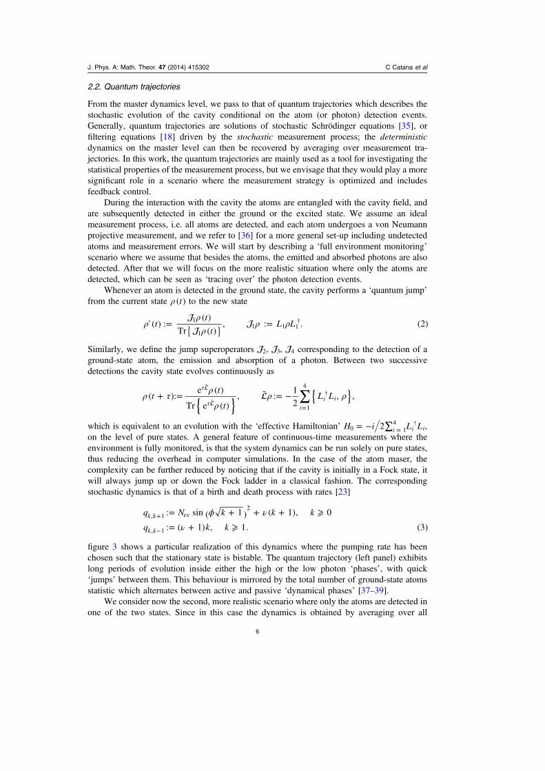
2.2. Quantum trajectories

From the master dynamics level, we pass to that of quantum trajectories which describes thestochastic evolution of the cavity conditional on the atom (or photon) detection events.Generally, quantum trajectories are solutions of stochastic Schrödinger equations [35], orfiltering equations [18] driven by the stochastic measurement process; the deterministicdynamics on the master level can then be recovered by averaging over measurement tra-jectories. In this work, the quantum trajectories are mainly used as a tool for investigating thestatistical properties of the measurement process, but we envisage that they would play a moresignificant role in a scenario where the measurement strategy is optimized and includesfeedback control.

During the interaction with the cavity the atoms are entangled with the cavity field, andare subsequently detected in either the ground or the excited state. We assume an idealmeasurement process, i.e. all atoms are detected, and each atom undergoes a von Neumannprojective measurement, and we refer to [36] for a more general set-up including undetectedatoms and measurement errors. We will start by describing a ‘full environment monitoring’scenario where we assume that besides the atoms, the emitted and absorbed photons are alsodetected. After that we will focus on the more realistic situation where only the atoms aredetected, which can be seen as ‘tracing over’ the photon detection events.

Whenever an atom is detected in the ground state, the cavity performs a ‘quantum jump’from the current state ρ t( ) to the new state

ρρ

ρρ ρ′ = =

{ }t

t

tL L( ) :

( )

Tr ( ), : . (2)1

11 1 1

†

Similarly, we define the jump superoperators , ,2 3 4 corresponding to the detection of aground-state atom, the emission and absorption of a photon. Between two successivedetections the cavity state evolves continuously as

∑ρ τ ρ

ρρ ρ+ = = −

τ

τ={ } { }t

t

tL L( ):

e ( )

Tr e ( ), ˜ :

1

2, ,

ii i

˜

˜1

4†

which is equivalent to an evolution with the ‘effective Hamiltonian’ = − ∑ =H i L L2 i i i0 14 † ,

on the level of pure states. A general feature of continuous-time measurements where theenvironment is fully monitored, is that the system dynamics can be run solely on pure states,thus reducing the overhead in computer simulations. In the case of the atom maser, thecomplexity can be further reduced by noticing that if the cavity is initially in a Fock state, itwill always jump up or down the Fock ladder in a classical fashion. The correspondingstochastic dynamics is that of a birth and death process with rates [23]

ϕ νν

= + + + ⩾= + ⩾

+

−

q N k k k

q k k

: sin ( 1 ) ( 1), 0

: ( 1) , 1. (3)k k ex

k k

, 12

, 1

figure 3 shows a particular realization of this dynamics where the pumping rate has beenchosen such that the stationary state is bistable. The quantum trajectory (left panel) exhibitslong periods of evolution inside either the high or the low photon ‘phases’, with quick‘jumps’ between them. This behaviour is mirrored by the total number of ground-state atomsstatistic which alternates between active and passive ‘dynamical phases’ [37–39].

We consider now the second, more realistic scenario where only the atoms are detected inone of the two states. Since in this case the dynamics is obtained by averaging over all

J. Phys. A: Math. Theor. 47 (2014) 415302 C Catana et al

6

unobserved photon events, the cavity state will be generally mixed and needs to be describedby a density matrix. The jump superoperators 1 and 2 are the same as above, but the theevolution between jumps has generator 0 which replaces ̃, and takes into account allphoton events

ρ ρ ρ ρ ρ= + − + −{ }L L L L L L L L N:1

2, .ex0 3 3

†4 4

†3†

3 4†

4

Let < <t t ...1 2 be a sequence of detection events occurring after the initial time t0, and let∈i {1, 2}k be the jump type for the atom detected at time tk. We denote by= t i t id {( , ),..., ( , )}t n n] 1 1 the detection record up to time t, with ⩽ < +t t tn n 1. If the initial

state of the field is ρ0, then the corresponding (un-normalized) quantum trajectory at time t isgiven by

ρ ρ= − − −−( )t d; e e ... e . (4)t

t ti

t ti i

t]

( ) ( )0

nn

n nn

0 0 11 1

0 1

The corresponding probability density is equal to ρ=p td d( ) Tr ( ( ; )),t t] ] and satisfies thenormalization condition

∫ ∫∑ ∑ ==

∞

∈ −( )

{ }p t td... d ... d 1.

n i it

t

t

t

t n

0 ,..., 1,2

] 1

nn

10 1

2.3. Simulations

In this section we briefly describe how to simulate the process which describes the stochasticevolution of the cavity (see section 2.2) in the time interval τ[0, ]. We are primarily interestedin the long time behaviour when the dynamics looses memory of the initial cavity state andtherefore, we can assume that its initial state is the stationary state ρss. Moreover, since thejump operators preserve the set of diagonal states, the probability p d( )t] can be computed byrestricting the attention to such states, rather than full density matrices. This reduces theproblem to that of simulating a birth and death process (the cavity state) together with twoprocesses describing the atoms counts.

Figure 3. In the full environment monitoring scenario, the cavity state evolves as a birthand death process on the Fock ladder. Left panel: when the stationary state is bistable(ϕ = 1.6, =N 16ex ) the state spends long periods in ‘phases’ with distinct mean photonnumbers, with quick ‘jumps’ between the phases. Right panel: histogram of the totalnumber of ground-state atoms (per unit of time) is bistable, exhibiting active andpassive dynamical phases.

J. Phys. A: Math. Theor. 47 (2014) 415302 C Catana et al

7

Denote by Λ ΛN t t t( ), ( ), ( )1 2 the -valued stochastic processes which describe the cavitystate at time t, the total number of ground-state and excited-state atoms detected up to time trespectively. The main steps of the algorithm are as follows.

Algorithm 1. Simulation of counting processes.

1. Set t = 0 and initialize N(t) by drawing randomly from ρ (·)ss i.e. ρ∼N (0) (·)ss ;

2. Simulate a birth and death process τ∈N t t{ ( ), [0, ]} with rates given in equation (3);3. Simulate a process which determines if the absorption of a photon was due to an atom or the bath;4. Simulate a Poisson process between two consecutive jumps of N t{ ( )} whose event times determinethe detection times of the excited atoms.

We now explain in detail how each of the steps is performed:

• Step 2 describes the evolution of the cavity state in the full environment monitoringscenario. Let < <s s ...1 2 denote the (random) times at which the cavity state makes ajump and Nk be the state of the cavity after the kth jump. Define

= − ∈ − +−J N N: { 1, 1}k k k 1 to be the increment indicating which type of jump (upor down) has occurred.

• Step 3 is carried out as follows: if = +J 1k then the cavity has absorbed a photon whichcan either come from an excited input atom or from the bath. To decide which of two typeof events has occurred we draw ∼C pBernoulli( )k with probability of a success (i.e. jumpwas due to an atom) equal to ν ϕ ν= + + + +( )( )p N N N N( 1)/ sin 1 ( 1)k ex k k

2 . Inaddition, we increment Λ t( )1 by one. If = −J 1k the cavity has emitted a photon in the bath,and no atom detection needs to be recorded.

• Step 4 the arrival times of the excited–state atoms in each time interval +s s[ , ]k k 1 aresimulated according to the event times of a Poisson process with state–dependentintensity ϕ +N Ncos ( 1 )ex k

2. Note that the Poisson processes for different intervals areasssumed to be independent and that the number of excited-atoms Λ t( )2 is equal to the tototal number of arrival times up to t.

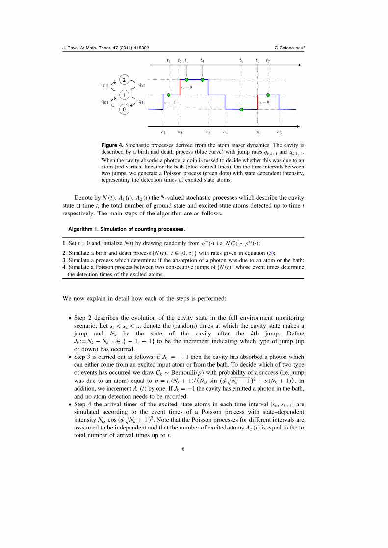
Figure 4. Stochastic processes derived from the atom maser dynamics. The cavity isdescribed by a birth and death process (blue curve) with jump rates +qk k, 1 and −qk k, 1.

When the cavity absorbs a photon, a coin is tossed to decide whether this was due to anatom (red vertical lines) or the bath (blue vertical lines). On the time intervals betweentwo jumps, we generate a Poisson process (green dots) with state dependent intensity,representing the detection times of excited state atoms.

J. Phys. A: Math. Theor. 47 (2014) 415302 C Catana et al

8

Finally, the arrival times of both ground and excited state atoms are collected in thesequence < <t t ...1 2 , and the type of atom arriving at tk is encoded in the label ∈i {1, 2}k .Figure 4 illustrates the above algorithm.

3. Classical and quantum statistical inference

In this section we review the basic notions and methods of statistical inference employed inthe present paper. We begin with an introduction to statistical inference for classical andquantum systems and then review a particular likelihood-free inference method used inBayesian statistics.

3.1. Basic notions of frequentist inference

Our starting point is the following basic statistical problem: given n independent identicallydistributed (i.i.d.) samples ∈X X,..., n1 drawn from a probability distribution θ whichdepends on an unknown parameter θ Θ∈ ⊂ p, we would like to construct an estimatorθ θ= X Xˆ : ˆ ( ,..., )n n n1 such that the ‘size’ of the estimation error θ θ−n̂ is as small as possible.The Cramér–Rao (CR) inequality states that the covariance matrix of any unbiased estimatorsatisfies the lower bound

⎜ ⎟⎡⎣⎢

⎛⎝

⎞⎠

⎤⎦⎥ θ θ θ θ θ− − ⩾ −( )n Iˆ ˆ ( ) ,n

Tn

1

where θI ( ) is the Fisher information matrix (for one sample) defined as

∫θθ θ

=∂

∂∂

∂θθ θ

>θ

I p xp x p x

x( ) ( )log ( ) log ( )

d , (5)ijp x i j( ) 0

with θp the density of θ with respect to some measure xd on . The importance of the CRbound lies in the fact that it is asymptotically achievable in the sense that there exist good (orefficient) estimators which satisfy the asymptotic normality property

θ θ θ− →

→∞−( ) ( )n N Ilim ˆ 0, ( ) , (6)

nn

1

where the limit convergence in law to the centred normal distribution θ −N I(0, ( ) )1 . Inparticular, under certain regularity conditions the MLE

∑θ =′ ′

θ Θθ∈

( )p Xˆ arg max logn

i

i

is an efficient estimator [40], which explains it popularity as a statistical estimation tool.Asymptotic normality is a general phenomenon which also holds for models with

dependent data, such as a (hidden) Markov process. Let ∈X( )n n be an ergodic Markov chainwith discrete states space =I m: {1 ,..., }, transition matrix = ∈T T( )i j i j I, , , and stationary dis-tribution π π π=: ( ,..., )m1 . As above, suppose that T depends on an unknown parameter

θ Θ∈ ⊂ p and we would like to estimate θ from the trajectory X X,..., n1 . In the long timelimit the process reaches stationarity, and the associated MLE θ̂n is again asymptoticallynormal, i.e. the limit (6) holds with the corresponding Fisher information (per unit of time)given by

J. Phys. A: Math. Theor. 47 (2014) 415302 C Catana et al

9

∑θ πθ

= =θ θ θ θ θ

≠( )I T ℓ ℓ T( ) : , :

d

dlog , (7)

i ji ij ij ij ij

2

where πθ is the stationary distribution at θ.Hidden Markov processes form an important class of statistical models extending the

notion of Markov process. Here we assume that the above Markov chain ∈X( )n n is notdirectly accessible, and the observations consist of another process ∈Y( )n n with values in

=J k{1 ,..., } such that Y Y,..., n1 are independent conditionally on X X,..., n1 and Yi dependsonly on Xi with conditional distribution given by

= = =( )Q Y y X x .i j i i,

The identifiability of the matrices T and Q is discussed in [41] and the asymptotic normalityof the MLE is discussed in [42] and in [43–45] for more general hidden Markov models. Inthis case the limiting Fisher information does not have a simple expression but it can beestimated from the data by the observed Fisher information given by

θ= −

∂∂

=θ

θ θ

θ θ=

( )( )( )I

n

ℓ Y Yℓ Y Y p Y Yˆ 1 ,...,

, ,..., log ,..., ,nn

n n

21

2ˆ

1 1

n

where θ̂ nis the MLE and θp Y Y( ,..., )n1 is the likelihood function for data Y Y,..., n1 . This

formula will be used later for estimating the Fisher information for the atom detection processin the atom maser.

3.2. Quantum statistics

In this section we give a very brief review of the key notions of quantum statical inferencethat are relevant for the paper. For more background reading we refer to [46–48].

3.2.1. Quantum state estimation. The standard quantum statistical problem is that of stateestimation or quantum tomography. Given a number of independent copies of a state ρθ

depending on an unknown parameter θ Θ∈ , we would like to estimate the parameter byperforming (separate or joint) measurements on the quantum systems and use the results toconstruct an estimator of θ.

If all measurements are identical and are characterized by the positive operator valuedmeasure (POVM) M(dx) over a space , then the measurement outcomes are i.i.d. withprobability distribution

ρ=θ θ( )x M xd ) Tr (d ) .M

The model θ Θ∈θ{ : }M has an associated classical Fisher information θI M( ; ) given by (5).If θ is one-dimensional, the optimal measurement can found by maximizing θI M( ; )

over all measurements M. A solution of this optimization is the measurement of theobservable θ called symmetric logarithmic derivative defined by the equation

ρθ

ρ ρ= +θθ θ θ θ( )

d

d

1

2.

The associated information is called the quantum Fisher information, it depends only on theintrinsic properties of the quantum statistical model ρ θ Θ∈θ{ : } and is equal to [46, 49]

J. Phys. A: Math. Theor. 47 (2014) 415302 C Catana et al

10

ρ ρ=θ θ θ{ }F ( ) Tr .2

Since θ depends on the unknown parameter θ, in practice one uses an adaptive two stepprocedure, where a small proportion of the systems are used to produce a rough estimate θ0 ofθ, and the observable θ0 is subsequently measured on the rest of the samples.Asymptotically, this procedure produces (maximum likelihood) estimators which areasymptotically normal, and achieve the quantum Fisher information in the sense of (6).

If θ θ θ=: ( ,..., )k1 is multidimensional, then the quantum Fisher information can bedefined in a similar way, using the SLDʼs θ i, corresponding to the coordinate θi. However,since these observables may not commute with each other, the quantum Fisher informationmay not be achievable by any measurement. One can find the asymptotically optimal solutionfor a given loss function (figure of merit) which is locally quadratic in θ, but in general theoptimal measurements for different loss functions are incompatible with each other [19]. Atheory extending the concept of asymptotic normality to the quantum set-up has beendeveloped in [50, 51], where it is shown how the n samples model converges to a quantumGaussian model with unknown mean and fixed covariance matrix. In this way the originalestimation problem can be transformed into the simpler problem of estimating the mean of aGaussian state.

3.2.2. System identification for quantum Markov processes. In this paper we are concernedwith the estimation of a one-dimensional parameter. However the quantum statistical modeldoes not consist of identically prepared, independent systems but is the (continuous time)output of a quantum Markov process. As in the case of classical Markov processes, the ‘data’is not iid but carries correlations due to the memory carried by the system.

The discrete time (ergodic) quantum Markov chain set-up was investigated in [19], and amore general treatment will be presented in [21]. For concreteness we can think of the atom-maser model illustrated in figure 1, with atoms passing at equal time intervals and theinteraction between atoms and system (cavity) given by a joint unitary transformation θUdepending on the unknown parameter θ. Two extreme scenarios can be considered. On theone hand, the experimenter can perform identical repeated measurements on the output, anduse the average of the results to estimate the unknown parameter. Such additive statistics areasymptotically normal and the corresponding Fisher information has an explicit expression.The other extreme is to consider the output as a quantum system whose state depends on theunknown parameter, and therefore has a quantum Fisher information. It turns out that the stateitself is asymptotically Gaussian in the statistical sense defined in [50, 51] and thecorresponding (asymptotic) quantum Fisher information has an explicit expression.

These results can be extended to continuous time [22], and the particular case of the atommaser was investigated in [23]. However the analysis in the latter work was based solely onthe total counts statistics and did not take into account the full atom measurement data, seesection 4.1 for more details. In the present work we fill this gap, and complement andcompare it with a likelihood-free method which uses a small number of statistics of the data,such as waiting time distribution and average number of successive detections of the sametype. The details of this method are described in the next section.

3.3. Approximate Bayesian computation

Similarly to the frequentist setting, Bayesian inference requires a sampling space and alikelihood θp x( | ), which can be seen as the conditional distribution of the data X given theparameter θ. Additionally, the Bayesian approach places a prior distribution with density π θ( )

J. Phys. A: Math. Theor. 47 (2014) 415302 C Catana et al

11

on the model parameters, which encodes our prior beliefs prior to seeing the data. Thelikelihood and the prior are then combined using Bayes theorem to derive the posteriordistribution which essentially is the conditional distribution of the (unknown) parameter θ,given the data ∈X

∫θ θ π θ

θ π θ θθ π θ= =

θ

p Xp X

p X

p X

p X( )

( ) ( )

( ) ( )d

( ) ( )

( ). (8)

The posterior distribution contains all the information about the parameters given theobserved data and therefore it is of high importance from a Bayesian viewpoint. Although inprinciple we are interested in deriving its probability density function explicitly, thecalculation of the normalizing constant in the denominator of (8) often makes such a taskdifficult. Traditionally, this has been a severe obstacle in Bayesian computation, especiallywhen θ is high-dimensional and the constant is analytically intractable.

Nevertheless, the last three decades have seen the development of several computationalmethods which enabled sampling-based Bayesian inference; that is to be able to draw samplesfrom θp X( | ) without the need of calculating p(X). For example, Markov Chain Monte–Carlo[52] methods provide such a tool to sample from the posterior distribution and obtain sampleestimates quantities of interest (e.g. densities, posterior moments etc), thereby performing theintegration implicitly.

When the likelihood can be either difficult or costly to evaluate it is practically infeasibleto use MCMC or even to perform maximum likelihood inference. However, provided it ispossible to simulate from a model, then ‘implicit’ methods such as ABC enable inferencewithout having to calculate the likelihood. These methods were originally developed forapplications in population genetics [53] and human demographics [54], but are now beingused in a wide range of fields including epidemiology, biology and finance, to name a few;see [24] and the references therein.

Intuitively, ABC methods involve simulating data from the model using various para-meter values and making inference based on which parameter values produced realizationsthat are ‘close’ to the observed data. It is easy to show that algorithm below generates exactsamples from the Bayesian posterior density θp X( | ) which is proportional to θ π θp X( | ) ( ):

Algorithm 2. Exact Bayesian computation (EBC).

1: Sample θ∗ from θp ( ).

2: Simulate dataset ∗X from the model using parameters θ∗.3: Accept θ∗ if =∗X X , otherwise reject.4: Repeat.

Clearly, the above algorithm is of practical use only if is a discrete space, since otherwisethe acceptance probability in step 3 is zero. For continuous distributions, or discrete ones inwhich the acceptance probability in step 3 is unacceptably low, [53] suggests the followingalgorithm:

Algorithm 3. Approximate Bayesian computation (ABC).

1: Sample ϕ∗ from π ϕ( ).

2: Simulate dataset ∗X from the model using parameters ϕ∗.3’: Accept ϕ∗ if ε⩽∗d s x s x( ( ), ( )) , otherwise reject.4: Repeat.

J. Phys. A: Math. Theor. 47 (2014) 415302 C Catana et al

12

Here d(·,·) is a distance function or metric, usually taken to be a type of Euclidian distance, s(·) is a function of the data, and ε is a tolerance. Note that s(·) can be the identity function butin practice, to give tolerable acceptance rate, it is usually taken to be a lower-dimensionalvector comprising some summary statistics that characterize key aspects of the data.

The output of the ABC algorithm is a sample from the ABC posterior density

θ θ ε= ⩽∗( )( ( ) ( ))p x p x d s x s x˜ ( ) , , .

If s (·) is a sufficient statistic, then the ABC posterior density converges to θp x( | ) as ε → 0[24]. However, in practice it is often difficult to find an s (·) which is sufficient. Hence ABCrequires a careful choice of s (·) and ε to make the acceptance rate tolerably large, at the sametime as trying not to make the ABC posterior too different from the true posterior θp x( | ).

In section 4.2 we will apply the ABC procedure for estimating the Rabi angle of the atommaser. For this, we will first discuss different choices of summary statistics and investigate towhat extent they enable us to recover the true posterior distribution. We will then show thatapplying ABC with a combination of the statistics gives a posterior which is comparable withthe performance of the MLE on the full data.

4. Results

We now return to the atom maser and apply the general frequentist and Bayesian methodsdescribed in the provious section to the problem of estimating the key dynamical parameter ofthe system, the Rabi angle ϕ. In [23] we have shown that the counts statistics Λ Λt t( ), ( )1 2 canbe used to estimate ϕ and we provided explicit expressions of the corresponding (asymptotic)Fisher informations per unit of time. Here we extend this investigation in two complementarydirections: i) we study the properties of the MLE for ϕ and the corresponding FisherInformation when the full atom detection record is taken into account, and ii) we illustratehow a suitable ABC algorithm enables to infer ϕ in a likelihood-free fashion, with a similarperformance to that of the full data MLE.

4.1. Likelihood based approaches to inference for the atom maser

We will first consider the problem of identifying the unknown parameter ϕ in the fullenvironment monitoring scenario (both atoms and emitted/absorbed photons are observed).Based on the description of the measurement processes outlined in section 2.3, one cancompute the likelihood function for a given measurement record and apply statistical tech-niques to investigate the asymptotic behaviour of the MLE [23]. Although we are not in an i.i.d. setting, the process consisting of the measurement record together with the conditionalcavity state is Markovian and ergodic, and the asymptotic normality results described insection 3.1 apply to this set-up. In particular, the Fisher information up to time t increaseslinearly in time in the sense that

= ≠→∞

I t

tIlim

( )0

t

and the mean square error of the MLE scales as I t1 ( · ). For simplicity we will call I theFisher information, but we should note that it is an asymptotic information per unit of time.As shown in [23] the Fisher information associated to the counting measurements in all fourchannels, achieves the upper bound given by the quantum Fisher information contained in thejoint quantum state of system (cavity) and output (atoms and photon bath) and is proportionalto the stationary mean photon number: ρ= =I I N N: 4 Tr ( )ex ssfull . This result will serve as a

J. Phys. A: Math. Theor. 47 (2014) 415302 C Catana et al

13

benchmark for assessing the power of other estimators constructed from the atoms detectionprocess which is accessible in experiments.

We switch now to the second scenario where the data consists solely of the atomsmeasurement record. Since we average over photon emission and absorption events, themeasurement process is not Markovian, but falls in the class of hidden Markov processes,where the observations (atom detections) are certain stochastic functionals of an unobservedMarkov process (the cavity).

Below we analyse two likelihood-based sub-scenarios. In the first one [23], all timecorrelations in the detection record are ignored and we only consider the total number ofcounts of a certain type up to time t, for which the Fisher information can be computedexplicitely. In the second sub-scenario we apply the maximum likelihood method to the fullatom counts record, and estimate the corresponding Fisher information.

4.1.1. Estimation based on total number of detections statistics. Let Λ Λ Λ=t t t( ) ( ( ), ( ))1 2 bethe two total number of counts up to time t, as defined in section 2.3. By applying the Markovproperty one can compute the characteristic function of Λ t( ) and prove that the processes are(jointly and locally) asymptotically normal [23]. More precisely, if ϕ ϕ= + u t0 then theproperly rescaled count statistics converge to a Gaussian distribution

Λ Λ μ− →ϕ( )( )t

t t N u V1

( ( )) ( , ), (9)0

where both μ μ ϕ= N( , )ex0 and ϕ=V V N( , )ex0 have explicit expressions in terms of certainLindblad type generators on the cavity space. Note that since ϕ is unknown, Λ t( ) is not‘centred’ by subtracting its expectation Λϕ t( ( )) as customary in the Central Limit Theorem,but with the expectation at the fixed parameter ϕ0. Consequently, the Gaussian limit has anon-zero mean which is proportional to the local parameter u.

From the Gaussian limit model we can easily obtain the Fisher information for differentcombinations of the count statistics. In particular the Fisher informations for the components

Figure 5. Fisher informations (per unit of time) for different count statistics as functionof ϕ, for =N 16ex : total number of ground state atoms (dash-dotted red curve), totalnumber of excited state atoms (dashed brown curve), optimal Fisher information(continuous blue curve).

J. Phys. A: Math. Theor. 47 (2014) 415302 C Catana et al

14

Λ1 and Λ2 are

μ μ= =I

VI

V, e1

12

11

22

22

and their dependence on ϕ0 is illustrated in figure 5 by the blue and red lines. By optimizingover the linear combinations Λ Λ+a t a t( ) ( )1 1 2 2 we obtain the maximum Fisher informationthat can be ’extracted’ from the total counts statistics

μ=∗

=

( )I

a

a Vamax . (10)a a

t

t1

2

t

The graphs of the three Fisher informations as functions of ϕ are shown in figure 5. We notethat all informations are equal to zero at a point ϕ ≈ 0.4 where the means of Λ Λ,1 2 arestationary with respect to ϕ.

4.1.2. Estimation based on the full likelihood. We now investigate the performance of theMLE and the corresponding Fisher information in the case where the full measurement recordup to time t is taken into account, rather that only the total counts. As outlined in section 2.2, adetection record = t i t id : {( , ),..., ( , )}t n n] 1 1 consists of a sequence of detection times prior totime t, together with labels indicating the outcome of each atom measurement. In simulations,such a record can be generated by following the procedure described in section 2.3. Byconstruction, this is a hidden Markov process, where the underlying Markov dynamics is thatof the cavity. The likelihood of the data dt] , seen as a function of ϕ, is

ρ=ϕp td d( ) Tr( ( ; )),t t] ] where ρ t d( ; )t] is the unnormalized cavity state defined in (4).For computing the MLE it is more convenient to work with the log-likelihood function

=ϕ ϕℓ pd d( ): log ( )t t] ] , which can be expressed as

∑ ρ ρ= +ϕ=

−−

−−( ) ( )( )ℓ d logTr e logTr e ,t

k

n

it t

kt t

n]

1

( )1

( )k

k k n0 1 0

where ρk denotes the conditional cavity state after the kth jump

ρρ

ρ=

−−

−−

−

−( )e

Tr e.k

it t

k

it t

k

( )1

( )1

kk k

kk k

0 1

0 1

Additionally, since the initial cavity state can be chosen to be the (diagonal) stationary stateρss, the jumps and semigroup calculations can be restricted to diagonal states (probabilitydistributions) which are truncate to a sufficiently large photon number. With these notations,the MLE is defined as

ϕ =′

′ϕ

ϕ ( )ℓ dˆ : arg max .t t]

Since the theoretical expression of the Fisher information Ifull involves a complicatedoptimization [44], we follow standard statistical methodology and use the observed Fisherinformation as an estimator of the theoretical one. The former is defined as minus the secondderivative of the log-likelihood function evaluated at the MLE

J. Phys. A: Math. Theor. 47 (2014) 415302 C Catana et al

15

ϕ= −

∂

∂ϕ

ϕ ϕ=

( )I

ℓ dˆ . (11)

tfull

2]

2

t̂

Figure 6 shows the average of the observed Fisher information over 150 trajectories (bluecurve) versus the optimal Fisher information I∗ contained in the total count statistics, definedin (10) . As expected, the former is always larger than the latter; more remarkably, the figureshows that the full measurement data is much more informative that the total counts statisticsin the region around the ϕ ≈ 0.4 where the mean photon number attains a local maximum andI∗ is equal to zero.

4.2. ABC for the atom-maser

In this section we apply the ABC procedure to the experimental data consisting of a set ofdetection events = t i t id : {( , ),..., ( , )}t n n] 1 1 , and different combinations from a total of 7summary statistics. The statistics fall into four categories: (i) total number of ground andexcited state atoms; (ii) waiting time statistics for both ground and excited state atoms; (iii)average number of the consecutive detections of the same type; (iv) a statistic of the localdensity of detected ground state atoms in the vicinity of detected excited atoms. For a betterphysical intuition we will give a brief description of each statistic, but we emphasize that noknowledge of their theoretical properties is required in applying the ABC estimationprocedure.

Furthermore, we employ different distance metrics for each type of summary statistic.For the total numbers of atoms we use the Euclidean distance, while for the average numberof consecutive detections the distance is defined as the absolute value of the differencedivided by the average number of consecutive detections in the experimental data. Whenusing the local density and the waiting time statistics we essentially need a metric whichmeasures the distance between two random samples. The Kolmogorov–Smirnov (KS)

Figure 6. The (estimated) Fisher information of the full measurement record Ifull (bluecurve) versus the Fisher information of the partial likelihood of the total countsstatistics I∗ (red curve) for =N 16ex . The former is much larger than the latter in theregion around ϕ ≈ 0.4 where ≈∗I 0.

J. Phys. A: Math. Theor. 47 (2014) 415302 C Catana et al

16

distance is often used to test whether two underlying one-dimensional probability distribu-tions differ. Therefore, we employed the statistic which is used for a Kolmogorov–Smirnovtest as our distance metric and is defined as follows.

Let X and Y be two random variables with distributions X and Y respectively. Denotetheir cumulative distribution functions (CDF) by = ⩽F x X x( ) ( )X and = ⩽G x Y x( ) ( )Y

respectively. Given n identically and independently distributed observations = …X X X( , , )n1

and = …Y Y Y( , , )n1 from X and respectively Y , we denote by Fn(x) and Gn(x) denote theempirical CDFs, i.e

∑ ∑= ==

⩽=

⩽{ } { }1 1F x n G y n( ) (1 ) , ( ) (1 ) .n

i

n

X x n

i

n

Y y

1 1i i

The KS distance between the two samples is defined as

= −( )( ) ( )X YKS F x G x( , ) sup .x

n n

The ABC algorithm we use is a slight variation on the general one described previously.For a given set of experimental data corresponding to a value of the unknown parameter ϕtrue

we perform a number = ×n 2 106 simulations for trial parameters ϕ ∈ [0.1, 1.5]trial drawnwith uniform probability. For each simulation we store the value of the parameter and thevalues of each of the 7 distances between the corresponding statistics of the simulated dataand the statistics of the experimental data. Let ϕ= =P i n{ , 1 ,..., }i

trial be the set of all the

simulated parameters and let = =D d i n{ , 1 ,..., }jij be the corresponding set of distances for

statistic ∈j {1 ,..., 7}. Let Dmj be the subset of Dj that contains the smallest 5% (corre-

sponding to a small ϵ) of the elements in Dj. Let ϕ= ∈P d D{ | }mj i

ij

mj

trial be the set of para-meters corresponding to the distances contained in Dm

j i.e. the values of the trial parameterwhich minimize the distance between the statistic j of the trial data and the experimental data.Finally, for statistic j, the set of accepted parameters Pm

j is used to build the correspondingposterior distribution.

In order to improve the resulting posterior distribution of the unknown parameter we alsoconsider combinations of two or more statistics. This boils down to finding the parameterswhich minimize the distances corresponding to all the chosen statistics. For example, whentwo statistics j and k are considered together, the resulting posterior distribution is built fromthe set ∩=P P Pm

jkmj

mk and is narrower than each individual posterior distribution. Following

this reasoning the best posterior distribution is obtained from the intersection of all 7 sets Pmj

and it is shown in figure 14.

4.2.1. Statistics of waiting times. We will call a waiting time, the time between twosuccessive detections of atoms in the same (ground or excited) state. In the stationary regime,the state of the cavity immediately after a jump of type i is on average given byρ ρ ρ= J J/Tr ( )i

ssi

ssafter , where ρ ρ= ∗L L( )i i i is the corresponding jump operator. This canbe seen as follows. Being an average state, it should be equal to the state after another jump,when averaging over all waiting times. The probability density of the waiting time, withinitial state ρ is ρ= − −p t( ) Tr( e ( ))i i

t( )i and the state after the jump is

ρ ρ= −t p t( ) e ( ) ( )it

i( )i . Therefore the average over time is

∫ ∫ρ ρ ρ ρ′ = = = −∞ ∞

− −( )( )p t t t t( ) ( )d e ( )d ( ).i it

i i0 0

1i

By identifying ρ and ρ′ we obtain the solution ρafter defined above. The corresponding waitingtime is

J. Phys. A: Math. Theor. 47 (2014) 415302 C Catana et al

17

ρ ρ= −( ) ( )( ) ( )( )p t( ) Tr e Tr . (12)i it

iss

issi

Let ϕF t( ; )iw( ) be the CDF of pi(t), where we have made explicit the dependance on the

unknown parameter ϕ. This dependence can be quantified by means of the Kolmogor-ov–Smirnov distance

ϕ ϕ ϕ ϕ= −⩾

( ) ( )KS F t F t, sup ( ; ) ;iw

ti

wi

w( )0

0

( ) ( )0

which is plotted in figure 7 as a function of ϕ, with ϕ = 0.440 and stationary initial state. Ingeneral when the KS distance is large, the parameter ϕ0 is easier to distinguish from ϕ andtherefore the accuracy of the ABC procedure is higher. A notable feature of figure 7 is the factthat the KS distance has two local minima, one for ϕ ϕ= 0 and a slightly larger one at a valuefor which the stationary cavity mean photon number is roughly the same as for ϕ0. Thisbehaviour is related to the vanishing of the classical Fisher information for total atom countsstatistics at ϕ = 0.4 as discussed in section 4.1.1.

We now apply ABC for the summary statistics given by the empirical waiting timedistribution, using the KS distance between such distributions as distance function. The ‘real’measurement data = t i t id : {( , ),..., ( , )}t n n] 1 1 is generated at ϕ = 0.44true and the syntheticdata is simulated for different values of ϕ, as detailed in algorithm 3. The result is theposterior distribution for this particular statistic, plotted in figure 8 against the likelihood

ϕp d( )t] , seen as posterior distribution of ϕ for a flat prior. As expected from the shape of thetheoretical values of the KS test of figure 7, the posterior distribution is broad and bimodal,and performs worse than the distribution of the maximum likelihood for the ‘experimentaldata’ (red curve).

4.2.2. Successive detector clicks. Another statistic of interest is the empirical mean ofsuccessive detections of atoms in the same (ground or excited) state, which is a measure ofcorrelations between the emerging atoms [55]. Since these correlations depend on the value ofϕ this easily computable statistic may constitute a suitable resource for estimation. The

Figure 7. The Kolmogorov–Smirnov distances between CDFs of the theoretical waitingtime distributions (red: ground state, blue: excited state) plotted as a function of ϕ atfixed ϕ = 0.440 (brown dotted line).

J. Phys. A: Math. Theor. 47 (2014) 415302 C Catana et al

18

theoretical mean in the stationary regime can be computed using the trajectories formalism[55]. The probability of the detected atom to be in the state ∈a {1, 2} when the detectorclicks once is

ρρ

=+( )

p a( )Tr{ }

Tr{ }.a

ss

ss1 2

Let p b a( | ) the probability of having an a detection at =t 00 followed by a b detection at anyfuture time moment with no other detections in between. This is given by

∫ ρρ

ρρ

=

= −

∞

−{ }

{ } { }

{ }

p b a t( ) d Tr e1

Tr

1

TrTr .

bt

ass

ass

ass b a

ss

0

01

0

Therefore the probability of having a sequence of two clicks a b, independent of time is givenby

ρ

ρ= = −+

−{ }({ })p ba p a p b a( ) ( ) ( )

1

TrTr .

ss b ass

1 20

1

In a similar manner we can compute the probability of more complex sequences of detections.Denote by p ba b( )n the probability of having n consecutive a detections in between two bdetections, and by p a( )n the probability of n consecutive a detections independent ofprevious or future detections. Then according to [55]

∑ = ==

∞

( ) ( ) ( )np ba bp a

p bp a

p b

p abp ba b

( )

( ),

( )

( ).

n

n n n

1

The average number of successive detections of type a is given by

∑ ρ

ρ= = = =

−

=

∞

−{ }( )

{ }n np a

p a

p ab p b a

( )

( )

1

( )

Tr

Tr.a

n

n ass

b ass

1 01

Figure 8. ABC posterior distribution for the waiting time statistics with ϕ = 0.44true ,

versus the likelihood ϕp d( )t] . Left panel: ground state waiting times; right panel:

excited state waiting times.

J. Phys. A: Math. Theor. 47 (2014) 415302 C Catana et al

19

In figure 9 we plot the theoretical values of the average number of detector clicks of thesame type as a function of ϕ for =N 16ex and ν = 0.1. The mean number of successiveground state atoms shows a strong peak at ϕ = 0.4 and is an informative statistic around thispoint, although it does not differentiate between values of ϕ which give the same rate ofproduction of ground state atoms. The mean number of excited state atoms is very high whenthe rate of these atoms is hign but varies little with ϕ beyond 0.4.

As before, we apply the ABC procedure for the ‘experimental data’= t i t id : {( , ),..., ( , )}t n n] 1 1 generated at ϕ = 0.5true , and the synthetic data is simulated for

different values of ϕ, as detailed in Algorithm 3.For each simulation run we compute the average numbers of succesive detector clicks of

the same type ⟨ ⟩n1sim and ⟨ ⟩n2

sim , and calculate their deviation from the averages obtained fromthe ‘experimental data’ ⟨ ⟩n1

exp , ⟨ ⟩n2exp by the relative distance

Figure 9.Average number of successive detections of atoms of a given type as functionof ϕ, for =N 16ex and ν = 0.1, for excited state atoms (blue line) and ground stateatoms (red line).

Figure 10. ABC posterior distribution for average number of detections of the sametype (histogram) at ϕ = 2true , for =N 16ex and ν = 0.1, versus the likelihood of the data

(red line). Left panel: ground state atoms. Right panel: excited state atoms.

J. Phys. A: Math. Theor. 47 (2014) 415302 C Catana et al

20

= − ∈dn

na1 , {1, 2}.a

a

a

sim

exp

Figure 10 shows the posterior distributions obtained from the ABC method for the averagenumber of consecutive detector clicks with the distance defined above. In the first case, thedistribution is more concentrated around the true value, but has a secondary peak at the pointwith the same mean.

4.2.3. Local density. We now consider a more complex statistic which takes into accountboth the arrival times and the number of detector clicks of ground state atoms. For eachexcited state atom arriving at a time t2i , we count how many ground state atoms have beendetected in the time interval −t s t( , )i i

2 2 . The local density is this number of atoms divided bythe length of the time interval s. For example the following set of detection events

= = = = = = == =

t t t t t t t

t t

0.1, 0.25, 0.37, 0.56, 0.82, 1.12, 1.21,

1.33, 1.67

11

21

31

41

51

62

72

81

92

has a vector of local densities = = =l l l{ 4, 4, 2}6 7 9 for s = 1.An analytic expression for the probability distribution of the local density follows from

equation (12). First the probability of having no ground state atom in the time interval t(0, ) is

ρ= −{ }( )p t( ) Tr e .t ss10 1

We have chosen as initial state the stationary state motivated by lack of knowledge about theatoms detected before =t 00 . Similarly we find the probability of n detections of ground stateatoms between =t 00 and =t t1 , moment at which an excited atom was detected, reads

∫ ∫ ρ= − − − − −

−

−{ }( )( ) ( )( ) ( )p t t t( ) d ... d Tr d e ... e . (13)nt

t

t

nt t t t t ss

10

1 2 1 1n

n n n

1

1 1 1 1 1

Figure 11. ABC posterior distribution from local density of ground state atoms atϕ = 0.4true (histogram), versus the likelihood of the real data.

J. Phys. A: Math. Theor. 47 (2014) 415302 C Catana et al

21

According to our definition, the probability of a given local density n t is =p n t( / )p t

t

( )in

.However, these theoretical probabilities are difficult to compute numerically and therefore weswitch to the Bayesian approach.

When applying ABC for this particular statistic we use as distance the Kolmogor-ov–Smirnov test. In figure 11 we show the posterior distribution for this statisticfor ϕ = 0.4true .

4.2.4. Statistics of total counts. The distribution of the total number of detections of atoms instate ∈a {1, 2} is similar to (13)

∫ ∫ ρ= − − − − −

−

−{ }( )( ) ( )( ) ( )p t t t( ) d ... d Tr e e ... e . (14)an

t

t

t

nt t

at t

at ss

01

n

a n a n n a

1

1 1

Even though these distributions can be cumbersome to compute numerically, it is easy to findthe average values of ground and excited atoms rates from energy balance considerations as

ν⟨ ⟩ −N and respectively ν− ⟨ ⟩ +N Nex , where ⟨ ⟩N is the average number of photons in thecavity in the stationary state shown in figure 2.

We apply the ABC procedure and compare the total number of atom counts in the trialsimulation, with the corresponding experimental values. The resulting posterior distributionsare shown in figure 12, for ϕ = 0.4true .

Close to the value ϕ = 0.4 the rate of emerging ground state atoms is at its maximum andtherefore, locally in the space of parameters, the asymptotic Fisher information per unit oftime, for the statistic of total counts vanishes as we have shown in the previous section and infigure 5. This also leads to a broad posterior distribution for the ABC method as seen infigure 12.

4.2.5. Combined statistics. As we have see, each individual statistic has a limited statisticalpower, and the corresponding posterior distribution is significantly broader than thelikelihood. Putting two or more of the statistics together gives more information about the trueparameter and improves the posterior distribution. Practically, this boils down to taking theintersection of the sets of parameters that minimize the corresponding tests as discussed insection 4.2. In figure 13 we plot the posterior for pairs of statistics taken together and remarkthat the distribution gets closer to the exact posterior. The improvement in the posteriordistribution varies with the choices of statistics to be taken together. For instance, the waiting

Figure 12. ABC posterior distribution for total counts (histogram) at ϕ = 0.40true ,

versus the likelihood of the data (red line).

J. Phys. A: Math. Theor. 47 (2014) 415302 C Catana et al

22

times statistics and the total number of detections look similar as they are both influenced bythe rate of atoms in a given state while the statistics of the local density and average numbersof consecutive detections of the same type are quite different.

In the end the most informative ABC procedure is to look at all the tests together, i.e.consider the posterior distribution for the intersection of all the 7 sets. This is shown as ahistogram in figure 14, and turns out to be only slightly broader than the likelihood of the realdata (red line), the latter being the posterior distribution for a flat prior.

5. Conclusions

In this article we have analysed and compared two different statistical methods for identifyinga dynamical parameter of a quantum open system, MLE and ABC. The two methods wereapplied to the estimation of the Rabi angle of the atom maser, from the measurement datagiven by the arrival times and states of the outgoing atoms. This particular model of an openquantum system was chosen due to its tractable probabilistic properties and its interestingphysical features: its dynamics is highly nonlinear with respect to the estimated parameter,and and the measurement record defines a hidden Markov process.

Figure 13. ABC posterior distribution for combined sets of statistics (histogram) atϕ = 0.44true , versus the likelihood of the data (red line). Top left: waiting times

statistics; top right: counts statistics; bottom: both waiting times and total countstogether.

J. Phys. A: Math. Theor. 47 (2014) 415302 C Catana et al

23

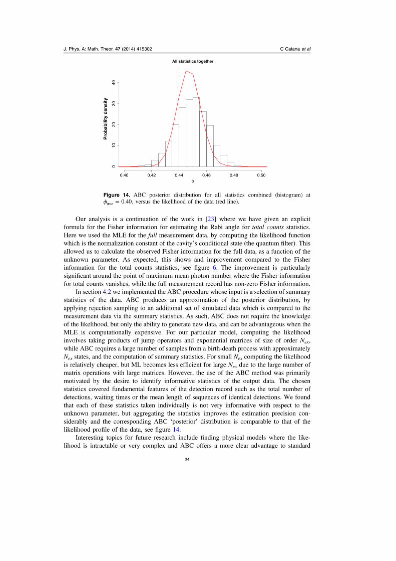
Our analysis is a continuation of the work in [23] where we have given an explicitformula for the Fisher information for estimating the Rabi angle for total counts statistics.Here we used the MLE for the full measurement data, by computing the likelihood functionwhich is the normalization constant of the cavityʼs conditional state (the quantum filter). Thisallowed us to calculate the observed Fisher information for the full data, as a function of theunknown parameter. As expected, this shows and improvement compared to the Fisherinformation for the total counts statistics, see figure 6. The improvement is particularlysignificant around the point of maximum mean photon number where the Fisher informationfor total counts vanishes, while the full measurement record has non-zero Fisher information.

In section 4.2 we implemented the ABC procedure whose input is a selection of summarystatistics of the data. ABC produces an approximation of the posterior distribution, byapplying rejection sampling to an additional set of simulated data which is compared to themeasurement data via the summary statistics. As such, ABC does not require the knowledgeof the likelihood, but only the ability to generate new data, and can be advantageous when theMLE is computationally expensive. For our particular model, computing the likelihoodinvolves taking products of jump operators and exponential matrices of size of order Nex,while ABC requires a large number of samples from a birth-death process with approximatelyNex states, and the computation of summary statistics. For small Nex computing the likelihoodis relatively cheaper, but ML becomes less efficient for large Nex due to the large number ofmatrix operations with large matrices. However, the use of the ABC method was primarilymotivated by the desire to identify informative statistics of the output data. The chosenstatistics covered fundamental features of the detection record such as the total number ofdetections, waiting times or the mean length of sequences of identical detections. We foundthat each of these statistics taken individually is not very informative with respect to theunknown parameter, but aggregating the statistics improves the estimation precision con-siderably and the corresponding ABC ‘posterior’ distribution is comparable to that of thelikelihood profile of the data, see figure 14.

Interesting topics for future research include finding physical models where the like-lihood is intractable or very complex and ABC offers a more clear advantage to standard

Figure 14. ABC posterior distribution for all statistics combined (histogram) atϕ = 0.40true , versus the likelihood of the data (red line).

J. Phys. A: Math. Theor. 47 (2014) 415302 C Catana et al

24

likelihood based methods, estimating large dimensional parameters, and exploring the rela-tionship between informative summary statistics and dimensional reduction methods [56, 57].

Acknowledgements

The authors acknowledge the use of Nottingham Universityʼs High Performance Computerfor performing the simulations involved in our study. This work was supported by the EPSRCFellowship EP/E052290/1, and the EPSRC grant EP/J009776/1.

References

[1] Ljung L 1999 System Identification: Theory for the User (Englewood Cliffs, NJ: Prentice-Hall)[2] Fujiwara A 2001 Quantum channel identification problem Phys. Rev. A 63 042304[3] Burgarth D, Maruyama K and Nori F 2011 Indirect quantum tomography of quadratic

Hamiltonians New J. Phys. 13 013019[4] Cole J, Schirmer S, Greentree A, Wellard C, Oi D and Hollenberg L 2005 Identifying an

experimental two-state Hamiltonian to arbitrary accuracy Phys. Rev. A 71 062312[5] Howard M, Twamley J, Wittmann C, Gaebel T, Jelezko F and Wrachtrup J 2006 Quantum process

tomography and Linblad estimation of a solid-state qubit New J. Phys. 8 33[6] Dowling J P and Milburn G J 2003 Quantum technology: the second quantum revolution Phil.

Trans. R. Soc. A 361 1655–74[7] Mabuchi H and Khaneja N 2005 Principles and applications of control in quantum systems Int. J.

Robust Nonlinear Control 15 647–67[8] Kiilerich A H and Mølmer K 2014 Estimation of atomic interaction parameters by photon counting

Phys. Rev. A 89 052110[9] Mabuchi H 1996 Dynamical identification of open quantum systemsQuantum Semiclass. Opt. 8 1103–8[10] Gambetta J and Wiseman H M 2001 State and dynamical parameter estimation for open quantum

systems Phys. Rev. A 64 042105[11] Gammelmark S and Mølmer K 2013 Bayesian parameter inference from continuously monitored

quantum systems Phys. Rev. A 87 032115[12] Gardiner C and Zoller P 2004 Quantum Noise (Berlin: Springer)[13] Wiseman H M and Milburn G J 2009 Quantum Measurement and Control (Cambridge:

Cambridge University Press)[14] Breuer H-P and Petruccione F 2002 The Theory of Open Quantum Systems (Oxford: Oxford

University Press)[15] Parthasarathy K R 1992 An Introduction to Quantum Stochastic Calculus (Basel: Birkhauser)[16] Lindblad G 1976 On the generators of quantum dynamical semigroups Commun. Math. Phys. 48 119–30[17] Gorini V, Kossakowski A and Sudarshan E C G 1976 Completely positive semigroups of N-level

systems J. Math. Phys. 17 821–5[18] Belavkin V P 1992 Quantum stochastic calculus and quantum nonlinear filtering J. Multivariate

Anal. 42 171–201[19] Guţă M 2011 Fisher information and asymptotic normality in system identification for quantum

Markov chains Phys. Rev. A 83 062324[20] Gammelmark S and Mølmer K 2014 Fisher information and the quantum Cramér–Rao sensitivity

limit of continuous measurements Phys. Rev. Lett. 112 170401[21] Guţă M and Kiukas J Equivalence classes and local asymptotic normality in system identification

for quantum Markov chains Commun. Math. Phys. (arXiv:1402.3535) at press[22] Catana C, Guţă M and Bouten L 2014 Local asymptotic normality for quantum Markov processes

arXiv:1407.5131[23] Catana C, van Horssen M and Guţă M 2012 Asymptotic inference in system identification for the

atom maser Phil. Trans. R. Soc. A 370 5308–23[24] Marin J M, Pudlo P, Robert C and Ryder R 2012 Approximate Bayesian computational methods

Stat. Comput. 22 1009–20[25] Ferrie C and Granade C E 2014 Likelihood-free methods for quantum parameter estimation Phys.

Rev. Lett. 112 130402

J. Phys. A: Math. Theor. 47 (2014) 415302 C Catana et al

25

[26] Meschede D, Walther H and Muller G 1985 One-atom maser Phys. Rev. Lett. 54 551–3[27] Englert B-G, Loffler M, Benson O, Varcoe B, Weidinger M and Walther H 1998 Entangled atoms

in micromaser physics Fortschr. Phys. 46 897–926[28] Jaynes E T and Cummings F W 1963 Comparison of quantum and semiclassical radiation theories

with application to the beam maser Proc. IEEE 51 89–109[29] Englert B-G, Gantsog T, Schenzle A, Wagner C and Walther H 1996 One-atom maser: phase-

sensitive measurements Phys. Rev. A 53 4386–99[30] Bergou J, Davidovich L, Orszag M, Benkert C, Hillery M and Scully M O 1989 Role of pumping

statistics in a maser and laser dynamics: density-matrix approach Phys. Rev. A 40 5073–80[31] Guerra E S, Khoury A Z, Davidovich L and Zagury N 1991 Role of pumping statistics in

micromasers Phys. Rev. A 44 7785–96[32] Herzog U 1995 Micromaser with stationary non-Poissonian pumping Phys. Rev. A 52 602–18[33] Englert B-G and Morigi G 2002 Five Lectures on Dissipative Master Equations Lecture Notes in

Physics: Coherent evolution in noisy environments vol 611 (Berlin: Springer) pp 55–106 Chapter 6[34] Meystre P, Rempe G and Walther H 1988 Very-low-temperature behaviour of a micromaser Opt.

Lett. 13 73–104[35] Bouten L, Guţă M and Maassen H 2004 Stochastic Schrödinger equations J. Phys. A: Math. Gen.

37 3189–209[36] Briegel H-J, Englert B-G, Sterpi N and Walther H 1994 One-atom maser: statistics of detector

clicks Phys. Rev. A 49 2962–85[37] van Horssen M and Guţă M 2013 Large deviations, central limit and quantum dynamical phase

transitions in the atom maser (arXiv:quant-ph/1206.4956v2)[38] Benson O, Raithel G and Walther H 1994 Quantum jumps of the micromaser field: dynamic

behaviour close to phase transition points Phys. Rev. Lett. 72 3506–9[39] Garrahan J P, Armour A D and Lesanovsky I 2011 Quantum trajectory phase transitions in the

micromaser Phys. Rev. E 84 021115[40] Young G A and Smith R L 2010 Essentials of Statistical Inference (Cambridge: Cambridge

University Press)[41] Petrie T 1969 Probabilistic functions of finite state Markov chains Ann. Math. Stat. 40 97–115[42] Baum L E and Petrie T 1966 Statistical inference for probabilistic functions of finite state Markov

chains Ann. Math. Stat. 37 1554–63[43] Leroux B G 1992 Maximum-likelihood estimation for hidden Markov models Stoch. Proc. Appl.

40 127–43[44] Douc R and Matias C 2001 Asymptotics of the maximum likelihood estimator for general hidden

markov models Bernoulli 7 381–420[45] Bickel P J, Ritov Y and Ryden T 1998 Asymptotic normality of the maximum likelihood estimator

for general hidden markov models Ann. Stat. 26 1614–35[46] Holevo A S 1982 Probabilistic and Statistical Aspects of Quantum Theory (Amsterdam: North-

Holland)[47] Barndorff-Nielsen O, Gill R D and Jupp P 2003 On quantum statistical inference J. R. Stat. Soc. B

65 775–816[48] Gill R D and Guţă M 2012 On asymptotic quantum statistical inference IMS Collect. 65 105–27[49] Braunstein S and Caves C 1994 Statistical distance and the geometry of quantum states Phys. Rev.

Lett. 72 3439–43[50] Guţă M and Kahn J 2006 Local asymptotic normality for qubit states Phys. Rev. A 73 052108[51] Guţă M and Jencova A 2007 Local asymptotic normality in quantum statistics Commun. Math.

Phys. 276 341–79[52] Gamerman D and Lopes H F 2006 Markov Chain Monte–Carlo: Stochastic Simulation for

Bayesian Inference (Boca Raton, FL: Chemical Rubber Company (CRC Press))[53] Pritchard J K, Seielstad M T, Perez-Lezaun A and Feldman M W 1999 Population growth of

human Y chromosomes: a study of Y chromosome microsatellites Mol. Biol. Evol. 16 1791–8[54] Beaumont M A, Zhang W and Balding D J 2002 Approximate bayesian computation in population

genetics Genetics 162 2025–35[55] Johnson D B and Schieve W C 2001 Detection statistics in the micromaser Phys. Rev. A 63 033808[56] van Handel R and Mabuchi H 2005 Quantum projection filter for a highly nonlinear model in

cavity QED J. Opt. B: Quantum Semiclass. Opt. 7 S226[57] Saul L K and Roweis S T 2003 Think globally, fit locally: unsupervised learning of low

dimensional manifolds J. Mach. Learn. Res. 4 119–55

J. Phys. A: Math. Theor. 47 (2014) 415302 C Catana et al

26