MAXIMUM PRINCIPLES, SLIDING TECHNIQUES AND APPLICATIONS TONONLOCAL EQUATIONS

JEROME COVILLE

ABSTRACT. This paper is devoted to the study of maximum principles holding for some nonlocaldiffusion operators defined on (half-) bounded domain and its applications to obtain the qualitativebehavior of solutions of some nonlinear problems. I show that, as in the classical case, the nonlocaldiffusion considered satisfies a weak and a strong maximum principle. Uniqueness and monotonic-ity of solutions of nonlinear equations are therefore expected as in the classical case. I first present asimple proof of this qualitative behavior and the weak/strong maximum principle. A optimal con-dition to have a strong maximum for operatorM[u] := J ? u − u is also obtained. The proofs ofthe uniqueness and monotonicity essentially relies on the sliding method and the strong maximumprinciple.

1. Introduction and Main results

This article is devoted to maximum principles and sliding techniques to obtain the uniquenessand the monotone behavior of the positive solution of the following problem

(1.1)

J ? u− u− cu′ + f(u) = 0 in Ωu = u0 in R \ Ω

where Ω ⊂ R is a domain, J is a continuous non negative function such that∫

R J(z) dz = 1 and fis a Lipschitz continuous function.

Such problem arises in the study of so-called Traveling Fronts ( solutions of the form u(x, t) =φ(x + ct)) of the following nonlocal phase-transition problem

(1.2)∂u

∂t− (J ? u− u) = f(u) in R× R+.

The constant c is called the speed of the front and is usually unknown. In such model, J(x− y)dyrepresent the probability of an individual at the position y to migrate to the position x, then theoperator

∫R J ? u − u can be viewed as a diffusion operator. This kind of equation was initially

introduced in 1937 by Kolmogorov, Petrovskii and Piskunov [23, 18] as a way to derive the Fisherequation (i.e (1.3) below with f(s) = s(1− s))

(1.3)∂U

∂t= Uxx + f(U) for (x,t) ∈ R× R+.

In the literature, much attention has been drawn to reaction-diffusion equations like (1.3), asthey have proved to give a robust and accurate description of a wide variety of phenomena,ranging from combustion to bacterial growth, nerve propagation or epidemiology. For moreinformations, we point the interested reader to the following articles and reference therein: [2, 4,5, 18, 20, 22, 23, 24, 30].

(1.1) can be seen as a nonlocal version of the well known semi-linear elliptic equation

(1.4)

u′′ − cu′ + f(u) = 0 in Ω,u = u0 in ∂Ω.

2000 Mathematics Subject Classification. Primary 35B50, 47G20; Secondary 35J60 .Key words and phrases. Nonlocal diffusion operators, maximum principles, sliding methods.The author was supported in part by the Ceremade- UniversitA c© Paris Dauphine and by the CMM-Universidad de

Chile on an Ecos-Conicyt project .1

When Ω = (r, R), it is well known [6, 7, 28] that the positive solution of (1.4) is unique andmonotone provided that u0(r) 6= u0(R) are zeros of f . More precisely, assume that u0(r) = 0 andu0(R) = 1 are respectively a sub and a super-solution of (1.4), then

Theorem 1.1. [6, 7, 28]Any smooth solution u of

(1.5)

u′′ − cu′ + f(u) = 0 in (r, R)u(r) = 0,u(R) = 1.

is unique and monotone.

Remark 1.1. The above theorem holds as well, if you replace 0 and 1 by any constant sub andsuper-solution of (1.5).

Remark 1.2. Obviously, by interchanging 0 and 1, u will be a decreasing function.

Since, (1.1) shares many properties with (1.4), we expect to obtain similar result. Indeed, as-sume that u0(r) = 0 and u0(R) = 1 are respectively a sub and a super-solution of (1.1), then onehas

Theorem 1.2.Let Ω = (r, R) for some real r < 0 < R and let J be such that [−b,−a] ∪ [a, b] ⊂ supp(J) ∩ Ω forsome constant 0 ≤ a < b. Then any smooth solution u of

(1.6)

J ? u− u− cu′ + f(u) = 0 in (r, R)u(x) = 0 for x ≤ r,u(x) = 1 for x ≥ R.

is unique and monotone.

Observe that in the nonlocal situation, we require more information on the function u since uis explicit outside Ω. This is due to the nature of the considered convolution operator.

For unbounded domain Ω, the situation is more delicate and according to Ω, we need furtherassumptions on f to characterize positive solutions u of (1.1). Two situations can occur, eitherΩ = R or Ω is a semi infinite interval (i.e. Ω = (−∞, r) or Ω = (r, +∞) for some real r). In thelatter case, assuming that 0 and 1 are a sub and a super-solution of (1.1) and f is non-increasingnear the value of 1, the positive solution u of (1.1) is unique and monotone. More precisely, wehave

Theorem 1.3.Assume that J satisfies J(a) > 0 and J(b) > 0 for some reals a < 0 < b. Let Ω = (r, +∞) for somer and let f be such that f non-increasing near 1. Then any smooth solution u of

(1.7)

J ? u− u− cu′ + f(u) = 0 in Ωu(x) = 0 for x ≤ r,u(+∞) = 1,

is unique and monotone.

By the notation u(+∞), I mean limx→+∞u. Observe that in this situation, there is no fur-ther assumption on Ω. Obviously, as for a bounded domain, sweeping 0 and 1 will changes themonotonic behavior of u provided f is non decreasing near 0.

Remark 1.3. With the adequate assumption on f , Theorem 1.3 holds as well for unbounded do-main of the form Ω = (−∞, r),.

When Ω = R, problem (1.1) is reduced to the well known convolution equation

(1.8)

J ? u− u− cu′ + f(u) = 0 in Ru(−∞) = 0,u(+∞) = 1,

2

which has been intensively studied see [1, 3, 8, 9, 12, 13, 14, 15, 16, 19, 26, 27, 29] and referencestherein. Observe that in this case, from the translation invariance, we can only expect uniquenessup to translation of the solution. Monotonicity and uniqueness issue has been fully investigatefor general bistable and monostable nonlinearities f with prescribed behavior nears 0 and 1 see[1, 3, 8, 9, 13, 14]. We sum up these results in the two following theorems:

Theorem 1.4. [3, 9, 13] (”bistable”)Let f be such that f(0) = 0 = f(1) and f non-increasing near 0 and 1. Assume that J is even.Then any smooth solution u of

(1.9)

J ? u− u− cu′ + f(u) = 0 in Ru(−∞) = 0,u(+∞) = 1,

is unique (up to translation) and monotone. Furthermore there exists unique couple (u, c) solu-tion of (1.9)

Theorem 1.5. [8, 26] (”monostable”)Let f be such that f(0) = f(1) = 0, f(s) > 0 in (0, 1), f ′(0) > 0 and f non-increasing near 1.Assume that J has compact support and even. Then any smooth solution u of

(1.10)

J ? u− u− cu′ + f(u) = 0 in Ru(−∞) = 0,u(+∞) = 1,

is unique (up to translation) and monotone.

Remark 1.4. In both situation, bistable or monostable, the behavior of u is governed by the as-sumption made on f near the value u(±∞).

Remark 1.5. All the above theorem stand if we replace 0 and 1 by any constant α and β which arerespectively a sub and super-solution of (1.1).

1.1. General comments.(1.2) appears also in other contexts, in particular in Ising model and in some Lattice model

involving discrete diffusion operator. I point the interested reader to the following references fordeeper explanations [3, 10, 24, 26, 29].

A significantly part of this paper is devoted to maximum and comparison principles holdingfor (1.5), (1.6) and some nonlinear operators. I obtain weak and strong maximum principle forthose problems. These maximum principles are analogue of the classical maximum principlesfor elliptic problem that we find in [21, 25].

I have so far only investigate the one dimensional case. Maximum and comparison principlesin multi-dimension for various type of nonlocal operators are currently under investigation andappears to be largely be an open question.

As a first consequence of this investigation on maximum principles, I obtain a generalizedversion of Theorem 1.2. More precisely, I prove

Theorem 1.6.Let Ω = (r, R) for some real r < 0 < R, g an increasing function and J be such that [−b,−a] ∪[a, b] ⊂ supp(J) ∩ Ω for some constant 0 ≤ a < b. Then any smooth solution u of

(1.11)

J ? g(u)− cu′ + f(u) = 0 in (r, R)u(x) = 0 for x ≤ r,u(x) = 1 for x ≥ R,

satisfying 0 < u < 1 is unique and monotone.

In this analysis, I also observe that provided an extra assumption on J , the proof of Theorem1.6 holds as well for the nonlinear density depending nonlocal operator∫

RJ(

x− y

u(y)) dy − u(x),

3

recently introduced by Cortazar, Elgueta and Rossi [11].Another consequence of this investigation is the generalization of Theorem 1.4. Indeed, in a

previous work [13], I have observe that Theorem 1.4 holds for linear operator L satisfying thefollowing properties:

(1) For all positive functions U , let Uh(.) := U(. + h). Then for all h > 0 we have L[Uh](x) ≤L[U ](x + h) ∀x ∈ R.

(2) Let v a positive constant then we have L[v] ≤ 0.(3) If u achieves a global minimum (resp.a global maximum) at some point ξ then the follow-

ing holds:• Either L[u](ξ) > 0 (resp. L[u](ξ) < 0)• Or L[u](ξ) = 0 and u is identically constant.

Such condition are easily verified by the operator J ? u − u when J is even. In this presentnote, I establish a necessary and sufficient condition on J to have the above conditions. This maytherefore generalized Theorem 1.4 for a new class of kernel.

1.2. Methods and plan.The techniques used to prove Theorems 1.2 and 1.3 are mainly based on an adaption to non-

local situation of the sliding techniques introduced by Berestycki and Nirenberg [6] to obtain theuniqueness and monotonicity of solutions of (1.4). These techniques crucially rely on maximumand comparison principles which hold for the considered operators. In the first two sections, Istudy some maximum principles and comparison principles satisfied by operators of the form:

(1.12)∫

Ω

J(x− y)u(y) dy − u

Then in the last two section, using sliding methods, I deal with the proof of Theorem 1.2 and 1.3.

2. Maximum principles

In this section, I prove several maximum principles holding for integrodifferential operatorsdefined respectively in bounded and unbounded domain. I have divided this section into twosubsections each of them devoted to Maximum principles in bounded domains and unboundeddomains. We start with some notation that we will constantly use along this paper. Let L,S,Mbe the following operators:

L[u] :=∫

Ω

J(x− y)u(y)dy − u + c(x)u, when Ω = (r, R),(2.1)

S[u] :=∫

Ω

J(x− y)u(y)dy − u, when Ω = (r, +∞) or Ω = (−∞, r),(2.2)

M[u] :=∫

RJ(x− y)u(y)dy − u := J ? u− u,(2.3)

where J ∈ C0(R) ∩ L1(R) so that∫

R J = 1 and c(x) ∈ C0(Ω) so that c(x) ≤ 0.

2.1. Maximum principles in bounded domains.Along this subsection, Ω will always refer to Ω = (r, R) for some r < R and L is defined by

(2.1). Let first introduce some functions that use along this subsection. Let α and β be two realsand let h−α and h+

β be defined by

h−α := α

∫ r

−∞J(x− y)dy,(2.4)

h+β := β

∫ ∞

R

J(x− y)dy.(2.5)

My first result is a weak maximum principle for L:4

Theorem 2.1. Weak Maximum PrincipleLet u ∈ C0(Ω) be such that

L[u] + h−α + h+β ≥ 0 in Ω,(2.6)

u(r) ≥ α,(2.7)

u(R) ≥ β.(2.8)

Thenmax

Ωu ≤ max

∂Ωu+.

Furthermore, if maxΩ u ≥ 0 then maxΩ u = max∂Ω u.

Remarks 2.1. Similarly if

L[u] + h−α + h+β ≤ 0 in Ω,(2.9)

u(r) ≤ α,(2.10)

u(R) ≤ β.(2.11)

Thenmin

Ωu ≥ min

∂Ωu−.

And if minΩ u ≤ 0 then minΩ u = min∂Ω u.

Proof of Theorem 2.1First, let h− and h+ be defined by

h− := u(r)∫ r

−∞J(x− y)dy,

h+ := u(R)∫ ∞

R

J(x− y)dy.

Next, extend u outside Ω the following way

(2.12) u(x) :=

u(x) in Ω,u(r) in (−∞, r),u(R) in (r,∞).

Observe that in Ω we have:

(2.13) M[u] + c(x)u = L[u] + h− + h+ ≥ (h− − h−α ) + (h+ − h+β ) ≥ 0.

Now observe that if the following inequality holds

(2.14) maxΩ

u ≤ maxR\Ω

u+,

then from the definition of u we get

maxΩ

u ≤ max∂Ω

u+.

So to prove Theorem 2.1, we are reduce to show (2.14).Define γ+ := maxu(r), u(R), then one has maxR\Ω u+ ≥ γ+.We argue now by contradiction. Assume that (2.14) does not hold, then u achieves a positivemaximum at some point x0 ∈ Ω and u(x0) = maxΩ u > γ+. By definition of u, we have u(x0) =maxR u > γ+. Therefore, at x0, u satisfies:∫

RJ(x0 − y)[u(y)− u(x0)] dy ≤ 0,(2.15)

c(x0)u(x0) ≤ 0.(2.16)

Combining now (2.15)-(2.16) with (2.13) we end up with

0 ≤ J ? u(x0)− u(x0)︸ ︷︷ ︸ + c(x0)u(x0)︸ ︷︷ ︸ ≤ 0

≤ 0 ≤ 05

Therefore

J ? u(x0)− u(x0) =∫

RJ(x0 − y)[u(y)− u(x0)] dy = 0.

Hence, ∀ y ∈ x0 − supp(J), u(y) = u(x0). In particular ∀ y ∈ x0 − [a, b], u(y) = u(x0) for somea < b. We have now the following alternative:

• Either (R \ Ω) ∩ (x0 − [a, b]) 6= ∅ and then we have a contradiction since there exits y ∈ Rsuch that either γ+ < u(x0) = u(y) = u(R) ≤ γ+ or γ+ < u(x0) = u(y) = u(r) ≤ γ+.

• Or (R \ Ω) ∩ (x0 − [a, b]) = ∅ and then (x0 − [a, b]) ⊂⊂ Ω.

In the later case, we can repeat the previous computation at the points x0 + b and x0 + a to obtain∀ y ∈ x0 − [2a, 2b], u(y) = u(x0). Again we have the alternative:

• Either (R \ Ω) ∩ (x0 − [2a, 2b]) 6= ∅ and then we have a contradiction.• Or (R \ Ω) ∩ (x0 − [2a, 2b]) = ∅ and then (x0 − [2a, 2b]) ⊂⊂ Ω.

By iterating this process, since Ω is bounded, we achieve for some positive integer n,

(R \ Ω) ∩ (x0 − [na, nb]) 6= ∅

and∀ y ∈ x0 − [na, nb], u(y) = u(x0),

which yields to a contradiction.In the case, maxΩ u > 0, following the above argumentation, we can prove that

(2.17) maxΩ

u ≤ maxR\Ω

u.

Hence,max∂Ω

u ≤ maxΩ

u ≤ maxR\Ω

u = max∂Ω

u.

Remark 2.1. Note that the weak maximum principle will also holds when h−α and h+β are replace

by any function g− and g+ satisfying h−α ≥ g− and h+β ≥ g+.

Remark 2.2. When c(x) ≡ 0, the assumption maxΩ u ≥ 0 is not needed to have

max∂Ω

u ≤ maxΩ

u ≤ maxR\Ω

u = max∂Ω

u.

Indeed it is needed to guaranties that (2.16) holds. When c(x) ≡ 0, (2.16) trivially holds.

Next, we give a sufficient condition on J and Ω such that L satisfies a strong maximum prin-ciple. Assume that J satisfies the following conditions

(H1) Ω ∩R+ 6= ∅ and Ω ∩ R− 6= ∅(H2) ∃ b > a ≥ 0 such that [−b,−a] ∪ [a, b] ⊂ supp(J) ∩ Ω

Then we have the following strong maximum principle

Theorem 2.2. Strong Maximum principleLet u ∈ C0(Ω) be such that

L[u] + h−α + h+β ≥ 0 in Ω (resp. L[u] + h−α + h+

β ≤ 0 in Ω),

u(r) ≥ α (resp. u(r) ≤ α),

u(R) ≥ β (resp. u(R) ≤ β).

Assume that J satisfies (H1-H2) then u may not achieve a non-negative maximum (resp. non-positive minimum) in Ω without being constant and u(r) = u(R).

From these two maximum principles we obtain immediately the following practical corollary:6

Corollary 2.1.Assume that J satisfies (H1-H2). Let u ∈ C0(Ω) be such that

L[u] + h−α + h+β ≥ 0 in Ω,

u(r) = α ≤ 0,u(R) = β ≤ 0.

Then

• Either u < 0• Or u ≡ 0.

Remarks 2.2.Similarly if L[u] ≤ 0, u(r) = α ≥ 0 and u(R) = β ≥ 0 then u is either positive or identically 0.

The proof of the corollary is a straightforward application of theses two theorems. Now let usprove the strong maximum principle.Proof of Theorem 2.2

The proof in the other cases being similar, I only treat the case of continuous function u satis-fying

L[u] + h−α + h+β ≥ 0 in Ω

u(r) ≥ αu(R) ≥ β.

Assume that u achieves a non-negative maximum in Ω at x0. Using the weak maximum prin-ciple yields to

u(x0) = maxu(r), u(R),u(x0) = u(x0) = max

Ωu = max

∂Ωu = max

R\Ωu,

where u is define by (2.12). Therefore, u achieves a global non-negative maximum at x0. To obtainu ≡ u(x0), we show that u ≡ u(x0). The later is obtained via a connexity argument.

Let Γ be the following setΓ = x ∈ Ω|u(x) = u(x0).

We will show that it is a nonempty open and closed subset of Ω for the induce topology.Since u is a continuous function then Γ is a closed subset of Ω. Let us now show that Γ is a

open subset of Ω. Let x1 ∈ Γ then u achieves a global non-negative maximum at x1. Arguing asin the proof of the weak maximum principle, we get

J ? u(x1)− u(x1) =∫

RJ(x1 − y)[u(y)− u(x1)] dy = 0.

Since u achieves a global maximum at x1, we have ∀ y ∈ R u(y) − u(x1) ≤ 0. Therefore ∀ y ∈x1 + supp(J), u(y) = u(x1). In particular ∀ y ∈ x1 + [−b,−a]∪ [a, b], u(y) = u(x1). We are leadto consider the two following cases:

• x1 + b ∈ Ω :In that case, we repeat the previous computation with (x1 + b) instead of x1 to get ∀ y ∈(x1 + b)+ [−b,−a]∪ [a, b], u(y) = u(x1). Now from the assumption on J and Ω, we havex1 + a ∈ Ω. Repeating the previous computation with x1 + a instead of x1, it follows that∀ y ∈ (x1 + a) + [−b,−a] ∪ [a, b], u(y) = u(x1). Combining these two results, yields to∀ y ∈ x1 + [−b + a, b− a], u(y) = u(x1).

• x1 + b 6∈ Ω :In that case, using the assumption on a and b, it easy to see that x1− b and x1−a are in Ω.Using the above arguments, we end up with ∀ y ∈ (x1−b)+ [−b,−a]∪[a, b], u(y) = u(x1)and ∀ y ∈ (x1 − a) + [−b,−a] ∪ [a, b], u(y) = u(x1). Again combining these two resultsyields to ∀ y ∈ x1 + [−b + a, b− a], u(y) = u(x1).

7

From both cases we have u(y) = u(x1) on (x1 + (−(b − a), (b + a))) ∩ Ω, which implies that Γ isan open subset of Ω.

Remark 2.3. Observe that the strong maximum principle relies on the possibility of ”covering” Ωwith closed sets.

When h−α +h+β has a sign, we can improve the strong maximum principle. Indeed, in that case

we have the following

Theorem 2.3.Let u ∈ C0(Ω) be such that

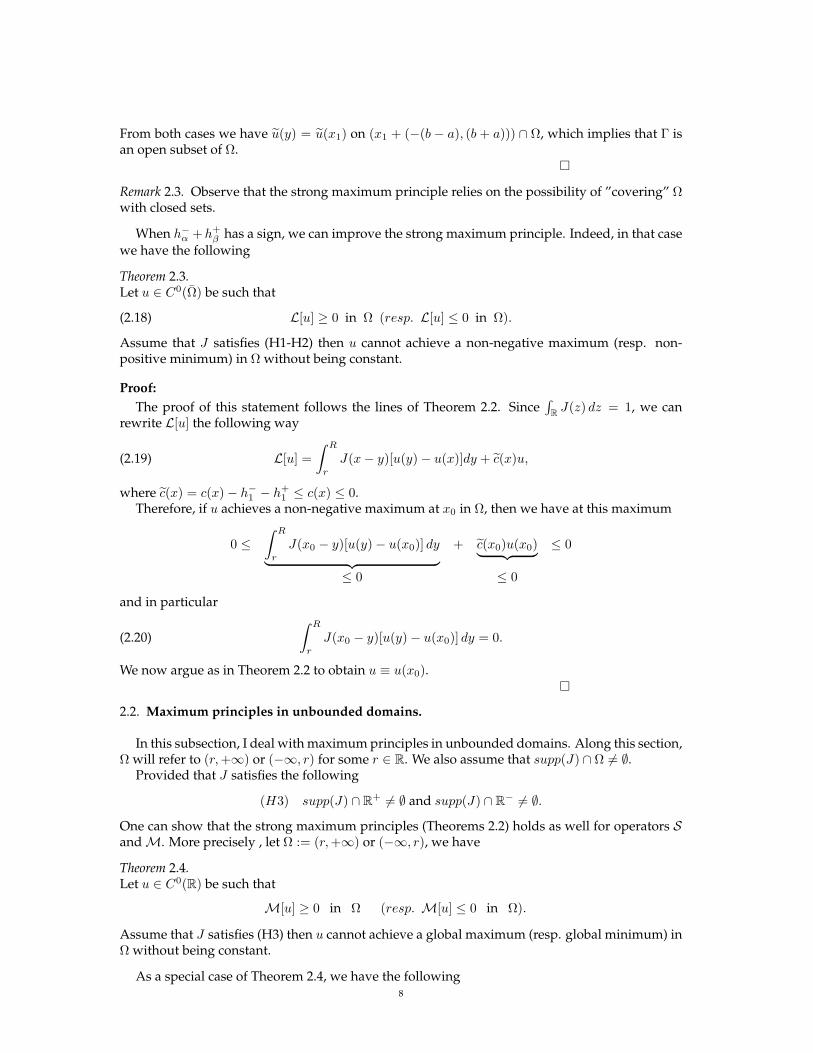
(2.18) L[u] ≥ 0 in Ω (resp. L[u] ≤ 0 in Ω).

Assume that J satisfies (H1-H2) then u cannot achieve a non-negative maximum (resp. non-positive minimum) in Ω without being constant.

Proof:The proof of this statement follows the lines of Theorem 2.2. Since

∫R J(z) dz = 1, we can

rewrite L[u] the following way

(2.19) L[u] =∫ R

r

J(x− y)[u(y)− u(x)]dy + c(x)u,

where c(x) = c(x)− h−1 − h+1 ≤ c(x) ≤ 0.

Therefore, if u achieves a non-negative maximum at x0 in Ω, then we have at this maximum

0 ≤∫ R

r

J(x0 − y)[u(y)− u(x0)] dy︸ ︷︷ ︸ + c(x0)u(x0)︸ ︷︷ ︸ ≤ 0

≤ 0 ≤ 0

and in particular

(2.20)∫ R

r

J(x0 − y)[u(y)− u(x0)] dy = 0.

We now argue as in Theorem 2.2 to obtain u ≡ u(x0).

2.2. Maximum principles in unbounded domains.

In this subsection, I deal with maximum principles in unbounded domains. Along this section,Ω will refer to (r, +∞) or (−∞, r) for some r ∈ R. We also assume that supp(J) ∩ Ω 6= ∅.

Provided that J satisfies the following

(H3) supp(J) ∩ R+ 6= ∅ and supp(J) ∩ R− 6= ∅.

One can show that the strong maximum principles (Theorems 2.2) holds as well for operators Sand M. More precisely , let Ω := (r, +∞) or (−∞, r), we have

Theorem 2.4.Let u ∈ C0(R) be such that

M[u] ≥ 0 in Ω (resp. M[u] ≤ 0 in Ω).

Assume that J satisfies (H3) then u cannot achieve a global maximum (resp. global minimum) inΩ without being constant.

As a special case of Theorem 2.4, we have the following8

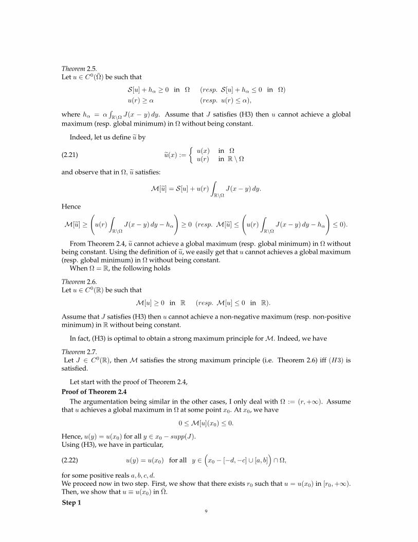
Theorem 2.5.Let u ∈ C0(Ω) be such that

S[u] + hα ≥ 0 in Ω (resp. S[u] + hα ≤ 0 in Ω)

u(r) ≥ α (resp. u(r) ≤ α),

where hα = α∫

R\Ω J(x − y) dy. Assume that J satisfies (H3) then u cannot achieve a globalmaximum (resp. global minimum) in Ω without being constant.

Indeed, let us define u by

(2.21) u(x) :=

u(x) in Ωu(r) in R \ Ω

and observe that in Ω, u satisfies:

M[u] = S[u] + u(r)∫

R\ΩJ(x− y) dy.

Hence

M[u] ≥

(u(r)

∫R\Ω

J(x− y) dy − hα

)≥ 0 (resp. M[u] ≤

(u(r)

∫R\Ω

J(x− y) dy − hα

)≤ 0).

From Theorem 2.4, u cannot achieve a global maximum (resp. global minimum) in Ω withoutbeing constant. Using the definition of u, we easily get that u cannot achieves a global maximum(resp. global minimum) in Ω without being constant.

When Ω = R, the following holds

Theorem 2.6.Let u ∈ C0(R) be such that

M[u] ≥ 0 in R (resp. M[u] ≤ 0 in R).

Assume that J satisfies (H3) then u cannot achieve a non-negative maximum (resp. non-positiveminimum) in R without being constant.

In fact, (H3) is optimal to obtain a strong maximum principle for M. Indeed, we have

Theorem 2.7.Let J ∈ C0(R), then M satisfies the strong maximum principle (i.e. Theorem 2.6) iff (H3) is

satisfied.

Let start with the proof of Theorem 2.4,Proof of Theorem 2.4

The argumentation being similar in the other cases, I only deal with Ω := (r, +∞). Assumethat u achieves a global maximum in Ω at some point x0. At x0, we have

0 ≤M[u](x0) ≤ 0.

Hence, u(y) = u(x0) for all y ∈ x0 − supp(J).Using (H3), we have in particular,

(2.22) u(y) = u(x0) for all y ∈(x0 − [−d,−c] ∪ [a, b]

)∩ Ω,

for some positive reals a, b, c, d.We proceed now in two step. First, we show that there exists r0 such that u = u(x0) in [r0,+∞).Then, we show that u ≡ u(x0) in Ω.

Step 19

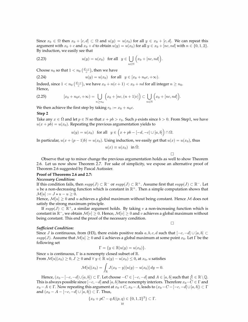
Since x0 ∈ Ω then x0 + [c, d] ⊂ Ω and u(y) = u(x0) for all y ∈ x0 + [c, d]. We can repeat thisargument with x0 + c and x0 + d to obtain u(y) = u(x0) for all y ∈ x0 + [nc, nd] with n ∈ 0, 1, 2.By induction, we easily see that

(2.23) u(y) = u(x0) for all y ∈⋃n∈N

(x0 + [nc, nd]

).

Choose n0 so that 1 < n0

(d−c

c

), then we have

(2.24) u(y) = u(x0) for all y ∈ [x0 + n0c,+∞).

Indeed, since 1 < n0

(d−c

c

), we have x0 + n(c + 1) < x0 + nd for all integer n ≥ n0.

Hence,

(2.25) [x0 + n0c,+∞) =⋃

n≥n0

(x0 + [nc, (n + 1)c]

)⊂⋃n∈N

(x0 + [nc, nd]

).

We then achieve the first step by taking r0 := x0 + n0c.Step 2Take any x ∈ Ω and let p ∈ N so that x + pb > r0. Such p exists since b > 0. From Step1, we haveu(x + pb) = u(x0). Repeating the previous argumentation yields to

u(y) = u(x0) for all y ∈(x + pb− [−d,−c] ∪ [a, b]

)∩ Ω.

In particular, u(x + (p− 1)b) = u(x0). Using induction, we easily get that u(x) = u(x0), thus

u(x) ≡ u(x0) in Ω.

Observe that up to minor change the previous argumentation holds as well to show Theorem

2.6. Let us now show Theorem 2.7. For sake of simplicity, we expose an alternative proof ofTheorem 2.6 suggested by Pascal Autissier.Proof of Theorems 2.6 and 2.7:Necessary Condition:If this condition fails, then supp(J) ⊂ R− or supp(J) ⊂ R+. Assume first that supp(J) ⊂ R−. Letu be a non-decreasing function which is constant in R+. Then a simple computation shows thatM[u] := J ? u− u ≥ 0.Hence, M[u] ≥ 0 and u achieves a global maximum without being constant. Hence M does notsatisfy the strong maximum principle.

If supp(J) ⊂ R+, a similar argument holds. By taking v a non-increasing function which isconstant in R−, we obtainM[v] ≥ 0. Hence,M[v] ≥ 0 and v achieves a global maximum withoutbeing constant. This end the proof of the necessary condition.

Sufficient Condition:Since J is continuous, from (H3), there exists positive reals a, b, c, d such that [−c,−d] ∪ [a, b] ⊂supp(J). Assume thatM[u] ≥ 0 and u achieves a global maximum at some point x0. Let Γ be thefollowing set

Γ = y ∈ R|u(y) = u(x0).Since u is continuous, Γ is a nonempty closed subset of R.From M[u](x0) ≥ 0, J ≥ 0 and ∀ y ∈ R u(y)− u(x0) ≤ 0, at x0, u satisfies

M[u](x0) =∫

RJ(x0 − y)[u(y)− u(x0)] dy = 0.

Hence, (x0− [−c,−d]∪ [a, b]) ⊂ Γ. Let choose−C ∈ [−c,−d] and A ∈ [a, b] such that AC ∈ R\Q.

This is always possible since [−c,−d] and [a, b] have nonempty interiors. Therefore x0−C ∈ Γ andx0−A ∈ Γ. Now repeating this argument at x0 +C, x0−A, leads to (x0−C− [−c,−d]∪ [a, b]) ⊂ Γand (x0 −A− [−c,−d] ∪ [a, b]) ⊂ Γ. Thus,

x0 + pC − qA|(p, q) ∈ 0, 1, 22 ⊂ Γ.10

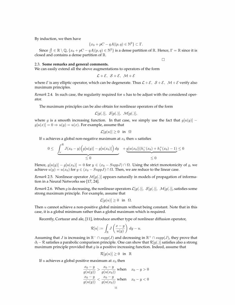
By induction, we then havex0 + pC − qA|(p, q) ∈ N2 ⊂ Γ.

Since AC ∈ R \Q, x0 + pC − qA|(p, q) ∈ N2 is a dense partition of R. Hence, Γ = R since it is

closed and contains a dense partition of R.

2.3. Some remarks and general comments.We can easily extend all the above augmentations to operators of the form

L+ E , S + E , M+ E

where E is any elliptic operator, which can be degenerate. Thus L+ E , S + E , M+ E verify alsomaximum principles.

Remark 2.4. In such case, the regularity required for u has to be adjust with the considered oper-ator.

The maximum principles can be also obtain for nonlinear operators of the form

L[g(.)], S[g(.)], M[g(.)],

where g is a smooth increasing function. In that case, we simply use the fact that g[u(y)] −g[u(x)] = 0 ⇒ u(y) = u(x). For example, assume that

L[g(u)] ≥ 0 in Ω

If u achieves a global non-negative maximum at x0 then u satisfies

0 ≤∫ R

r

J(x0 − y)(g[u(y)]− g[u(x0)]

)dy︸ ︷︷ ︸ + g[u(x0)](h−1 (x0) + h+

1 (x0)− 1)︸ ︷︷ ︸ ≤ 0

≤ 0 ≤ 0

Hence, g[u(y)] − g[u(x0)] = 0 for y ∈ (x0 − SuppJ) ∩ Ω. Using the strict monotonicity of g, weachieve u(y) = u(x0) for y ∈ (x0 − SuppJ) ∩ Ω. Then, we are reduce to the linear case.

Remark 2.5. Nonlinear operator M[g(.)] appears naturally in models of propagation of informa-tion in a Neural Networks see [17, 24].

Remark 2.6. When g is decreasing, the nonlinear operatorsL[g(.)], S[g(.)], M[g(.)], satisfies somestrong maximum principle. For example, assume that

L[g(u)] ≥ 0 in Ω.

Then u cannot achieve a non-positive global minimum without being constant. Note that in thiscase, it is a global minimum rather than a global maximum which is required.

Recently, Cortazar and ale, [11], introduce another type of nonlinear diffusion operator,

R[u] :=∫

RJ

(x− y

u(y)

)dy − u.

Assuming that J is increasing in R− ∩ supp(J) and decreasing in R+ ∩ supp(J), they prove that∂t−R satisfies a parabolic comparison principle. One can show thatR[g(.)] satisfies also a strongmaximum principle provided that g is a positive increasing function. Indeed, assume that

R[g(u)] ≥ 0 in R

If u achieves a global positive maximum at x0 then

x0 − y

g(u(y))>

x0 − y

g(u(x0))when x0 − y > 0

x0 − y

g(u(y))<

x0 − y

g(u(x0))when x0 − y < 0

11

Using the assumption made on J , we have for every y ∈ R,[J

(x0 − y

g(u(y))

)− J

(x0 − y

g(u(x0))

)]≤ 0.

Therefore u satisfies

0 ≤∫ +∞

−∞

[J

(x0 − y

g(u(y))

)− J

(x0 − y

g(u(x0))

)]dy ≤ 0

Hence, g[u(y)]− g[u(x0)] = 0 for y ∈ x0 − SuppJ . Using the strict monotonicity of g, we achieveu(y) = u(x0) for y ∈ x0−SuppJ . Then, we are reduce to the linear case. These density dependantoperator can be viewed as a nonlocal version of the classical porous media operator.

A consequence of the proofs of the strong maximum principle, is the characterisation of globalextremum of u. Namely, we can derive the following property

Lemma 2.1.Assume J satisfies (H3). Let u be a smooth (C0) function. If u achieves a global minimum (resp.aglobal maximum) at some point ξ then the following holds:

• Either M[u](ξ) > 0 (resp. M[u](ξ) < 0)• Or M[u](ξ) = 0 and u is identically constant.

Remark 2.7. An easy adaptation of the proof shows that Lemma 2.1 stands for u continuous byparts and with a finite number of discontinuities.

Remark 2.8. Lemma 2.1 holds as well for M+ E , L, L+ E , S, S + E and R, provided that theconsidered operator satisfies a strong maximum principle.

3. Comparison principles

In this section I deal with Comparison principles satisfied by operators L, S and M. Thisproperty comes often as a corollary of a maximum principle. Here we present two comparisonprinciples which are not a direct application of the maximum principle. The first is a linearcomparison principle, the second concerns a nonlinear comparison principle satisfied by S. Thissection is divided into two subsections, each one devoted to a comparison principle.

3.1. Linear Comparison principle.

Theorem 3.1. Linear Comparison PrincipleLet u and v be two smooth functions (C0(R)) and ω a connected subset of R. Assume that u andv satisfy the following conditions :

• M[v] ≥ 0 in ω ⊂ R• M[u] ≤ 0 in ω ⊂ R• u ≥ v in R− ω• if ω is an unbounded domain, assume also that lim∞ u− v ≥ 0.

Then u ≥ v in R.

Proof:Let first assume, that ω is bounded. Let w = u− v, so w will satisfy :• w ≥ 0, w 6≡ 0 in R− ω,• M[w] ≤ 0 in ω.

Let us define the following quantityγ := inf

R\ωw.

Now, we argue by contradiction. Assume that w achieves a negative minimum at x0. By assump-tion x0 ∈ ω and is a global minimum of w. So, at this point, w satisfies:

0 ≥M[w(x0)] = (J ? w − w)(x0) =∫

RJ(x0 − z)(w(z)− w(x0))dz ≤ 0.

12

It follows that w(y) = w(x0) on y − supp(J). Hence, for some reals a, b, we have the followingalternative:

• Either (R \ ω) ∩ (x0 − [a, b]) 6= ∅ and then we have a contradiction since there exits y ∈ Rsuch that 0 ≤ γ ≤ w(x0) = w(y) < 0.

• Or (R \ ω) ∩ (x0 − [a, b]) = ∅ and then (x0 − [a, b]) ⊂⊂ ω.In the later case, arguing as for the proof of Theorem 2.1, we can repeat the previous computationat the points x0 − b and x− a and using induction we achieve,

(R \ ω) ∩ (x0 − [na, nb]) 6= ∅,and

∀ y ∈ x0 − [na, nb], w(y) = w(x0),for some positive n ∈ N. Thus 0 ≤ γ ≤ w(x0) < 0, which is a contradiction.

In the case of ω unbounded, by assumption limx→∞ w ≥ 0, then there exists a compact subsetω1 such that x0 ∈ ω1 and w(x0) < infR\ω1 w. Then the above argument holds with R \ ω1 insteadof R \ ω.

3.2. Nonlinear Comparison Principle.In this subsection, I obtain the following nonlinear comparison principles,

Theorem 3.2. Nonlinear comparison principleAssume thatM defined by 2.3 verifies (H3), Ω = (r, +∞) for some r ∈ R and f ∈ C1(R), satisfies,f ′|(β,+∞) < 0. Let z and v smooth (C0(R)) functions satisfying,

M[z] + f(z) ≥ 0 in Ω,(3.1)

M[v] + f(v) ≤ 0 in Ω,(3.2)

limx→+∞z(x) ≤ β, limx→+∞v(x) ≥ β,(3.3)

z(x) ≤ α, v(x) ≥ α when x ≤ r.(3.4)

If in [r, +∞), z < β and v > α, then there exists τ ∈ R such that z ≤ vτ in R. Moreover, eitherz < vτ in Ω or z ≡ vτ in Ω.

Before proving Theorem 3.2, we start with some definitions of quantities that we will use allalong this subsection.

Let ε > 0 be such that f ′(s) < 0 for s ≥ β − ε. Choose δ ≤ ε4 positive, such that

(3.5) f ′(p) < −2δ ∀p such that β − p < δ.

If limx→+∞ z(x) = β, choose M > 0 such that :

β − v(x) <δ

2∀x > M,(3.6)

β − z(x) <δ

2∀x > M.(3.7)

Otherwise, we choose M such that

(3.8) v(x) > z(x) ∀x > M.

The proof of this theorem follows ideas developed by the author in [13] for convolution oper-ators. It essentially relies, on the following technical lemma which will be proved later on.

Lemma 3.1.Let z and v be respectively smooth positive sub and supersolution satisfying (3.1)-(3.4). If thereexists positive constant a ≤ δ

2 and b such that z and v satisfy:

v(x + b) > z(x) ∀x ∈ [r, M + 1],(3.9)

v(x + b) + a > z(x) ∀x ∈ Ω.(3.10)

13

Then we have v(x + b) ≥ z(x) ∀x ∈ R.

Proof of Theorem 3.2:Observe, that if infR v ≥ supR z then v ≥ z trivially holds. In the sequel, we assume that

infR v < maxR z.Assume for a moment that Lemma 3.1 holds. To prove Theorem 3.2, by construction of M and

δ, we just have to find an appropriate constant b which satisfies (3.9) and (3.10) and showing thateither vτ > z in Ω or z ≡ vτ in Ω.

Since v and z satisfy in [r, +∞): z < β and v > α, using (3.3)-(3.4) we can find a constant Dsuch that on the compact set [r, M + 1], we have for every b ≥ D

v(x + b) > z(x) ∀x ∈ [r, M + 1].

Now, we claim that there exists b ≥ D such that v(x + b) + δ2 > z(x) ∀x ∈ R.

If not then we have,

(3.11) ∀b ≥ D there exists x(b) such that v(x(b) + b) +δ

2≤ z(x(b)).

Since v ≥ α and v satisfies (3.4) we have

(3.12) v(x + b) +δ

2> z(x) for all b > 0 and x ≤ r.

Take now a sequence (bn)n∈N which tends to +∞. Let x(bn) be the point defined by (3.11).Thus we have for that sequence

(3.13) v(x(bn) + bn) +δ

2≤ z(x(bn)).

According to (3.12) we have x(bn) ≥ M + 1. Therefore the sequence x(bn) + bn converges to+∞. Pass to the limit in (3.13) to get

β +δ

2≤ lim

n→+∞v(x(bn) + bn) +

δ

2≤ lim sup

n→+∞z(x(bn)) ≤ β,

which is a contradiction. Therefore there exists a b > D such that

v(x + b) +δ

2> z(x) ∀x ∈ Ω.

Since we have found our appropriate constants a = δ2 and b, we can apply Lemma 3.1 to obtain

v(x + τ) ≥ z(x) ∀x ∈ R,

with τ = b. It remains to prove that in Ω either vτ > z or uτ ≡ v. We argue as follows. Letw := vτ − z, then either w > 0 in Ω or w achieves a non-negative minimum at some point x0 ∈ Ω.If such x0 exists then at this point we have w(x) ≥ w(x0) = 0 and

(3.14) 0 ≤M[w(x0)] ≤ f(z(x0))− f(v(x0 + τ)) = f(z(x0))− f(z(x0)) = 0.

Then using the argumentation in the proof of Theorem 2.4, we obtain w ≡ 0 in Ω, which meansvτ ≡ z in Ω. This ends the proof of Theorem 3.2.

Let now turn our attention to the proof of the technical Lemma 3.1.

Proof of Lemma 3.1:Let v and z be respectively a super and a subsolution of (3.1)-(3.4) satisfying (3.6) and (3.7) or

(3.8). Let a > 0 be such that

(3.15) v(x + b) + a > z(x) ∀x ∈ Ω.

Note that for b defined by (3.9) and (3.10), any a ≥ δ2 satisfies (3.15). Define

(3.16) a∗ = infa > 0 | v(x + b) + a > z(x) ∀x ∈ Ω.We claim that

14

Claim 3.1. a∗ = 0.

Observe that Claim 3.1 implies that v(x + b) ≥ z(x) ∀x ∈ Ω, which is the desired conclusion.Proof of claim 3.1

We argue by contradiction. If a∗ > 0, since limx→+∞ v(x + b) + a∗ − z(x) ≥ a∗ > 0 andv(x + b)− z(x) + a∗ ≥ a∗ > 0 for x ≤ r, there exists x0 ∈ Ω such that v(x0 + b) + a∗ = z(x0).Let w(x) := v(x + b) + a∗ − z(x), then

(3.17) 0 = w(x0) = minR

w(x).

Observe that w also satisfies the following equations:

M[w] ≤ f(z(x))− f(v(x + b))(3.18)w(+∞) ≥ a∗(3.19)

w(x) ≥ a∗ for x ≤ r.(3.20)

By assumption, v(x + b) > z(x) in (−∞,M + 1]. Hence x0 > M + 1.Let us define

(3.21) Q(x) := f(z(x))− f(v(x + b)).

Computing Q(x) at x0, it follows

(3.22) Q(x0) = f(v(x0 + b) + a∗)− f(v(x0 + b)) ≤ 0,

since x0 > M + 1 f is non-increasing for s ≥ β − ε, a∗ > 0 and β − ε < β − δ2 ≤ v for x > M .

Combining (3.18),(3.17) and (3.22) yields to

0 ≤M[w(x0)] ≤ Q(x0) ≤ 0.

Following the argumentation of Theorem 2.4, we end up with w = 0 in Ω which contradicts(3.19). Hence a∗ = 0, which ends the proof of Claim 3.1.

Remark 3.1. The previous analysis only holds for linear operators. It fails for operators such asM[g(.)] or R.

Remark 3.2. The regularity assumption on f can be improved. Indeed, the above proof holds aswell with f continuous and non-increasing in (β − ε,+∞) for some positive ε.

4. Sliding techniques and applications

In this section, using sliding techniques, I prove uniqueness and monotonicity of positive so-lution of the following problem:∫ R

r

J(x− y)g(u(y)) dy + f(u) + t−α + t+β = 0 in Ω(4.1)

u(r) = α(4.2)

u(R) = β,(4.3)

where t−α = g(α)∫ r

−∞ J(x − y)dy, t+β = g(β)∫∞

RJ(x − y)dy, g is an increasing function. We also

assume that f is continuous functions and that J satisfies (H1−H2). More precisely, I prove thefollowing,

Theorem 4.1.Let α < β. Assume that f ∈ C0. Then any solution u of (4.1)-(4.3), satisfying α < u < β, ismonotone increasing. Furthermore, this solution if its exists is unique.

15

Similarly, if α > β, then any solution u of (4.1)-(4.3), satisfying β < u < α, is monotonedecreasing. Observe that Theorem 1.2 comes as a special case of Theorem 4.1. Indeed, chooseg = Id, then a short computation shows that∫ R

r

J(x− y)g(u(y)) dy =∫ R

r

J(x− y)u(y) dy = L[u] + u,

t−α = h−α ,

t+β = h+β ,

where L is defined by (2.1) with c(x) ≡ 0. Hence, in this special cases (4.1)-(4.3) becomes

L[u] + f(u) + h−α + h+β = 0 in Ω

u(r) = α

u(R) = β,

where f(u) := f(u) + u.Before going to the proof defined for convenience the following nonlinear operator

(4.4) N [v] :=∫ +∞

−∞J(x− y)g(v(y))dy

Proof of Theorem 4.1:We start by showing that u is monotone.

4.1. Monotonicity.Let us define the following continuous extension of u:

(4.5) u(x) :=

u(x) in Ωu(r) in (−∞, r)u(R) in (R,+∞).

Observe that in Ω, u satisfies

(4.6)

N [u] + f(u) = 0 in Ω

u(x) = α for x ∈ (−∞, r]

u(x) = β for x ∈ [R,+∞)

Showing that u is monotone increasing in Ω will imply that u is monotone increasing. To obtainthat u is monotone increasing, we use a slidding technique developed by Berestycki and Niren-berg [6], which is based on comparison between u and its translated uτ := u(x + τ). We showthat for any positive τ we have u < uτ in Ω. First, observe that uτ satisfies

(4.7)

N [uτ ] + f(uτ ) = 0 in (r − τ,R− τ)

uτ (x) = α for x ∈ (−∞, r − τ ]

uτ (x) = β for x ∈ [R− τ,+∞)

Now let us define

(4.8) τ∗ = infτ ≥ 0|∀τ ′ ≥ τ, uτ ′ > u in ΩObserve that τ∗ is well defined since for any τ > R − r, by assumption and the definition of

u, we have u ≤ uτ in R and u < uτ in Ω. Hence τ∗ ≤ R − r. We now show that τ∗ = 0. Observethat by proving the claim below we obtain the monotonicity of the solution u.

Claim 4.1. τ∗ = 0

Proof of the claim:We argue by contradiction. Assume that τ∗ > 0, then since u is a continuous function, we will

have u ≤ uτ∗ in R. Let w := uτ∗ − u. From the definition of τ∗ and the continuity of u, w must16

achieve a non positive minimum at some point x0 in Ω. Namely, since w ≥ 0, we have w(x0) = 0.We are now lead to consider the following two cases:

• Either x0 ∈ [R− τ∗, R)• Or x0 ∈ (r, R− τ∗)

We will see that in both case we end up with a contradiction.First assume that x0 ∈ [R − τ∗, R). Since τ∗ > 0, using the definition of u we have uτ∗ ≡ β in[R− τ∗, R). We therefore get a contradiction since 0 = w(x0) = β − u(x0) > 0.

In the other case, w achieves its minimum in (r, R − τ∗). Now, using (4.6) and (4.7), at x0, wehave:

(4.9) N [uτ∗ ]−N [u] =∫ +∞

−∞J(x0 − y)[g(uτ∗(y))− g(u(y))] dy = 0

Since, g is increasing and uτ∗ ≥ u, it follows that g(uτ∗(y)) − g(u(y)) = 0 for all y ∈ x0 −Supp(J). Using the monotone increasing property of g yields to w(y) = uτ∗(y)− u(y) = 0 for ally ∈ x0−Supp(J). Arguing now as in Theorem 2.2, we end up with w ≡ 0 in all [r, R−τ∗]. Hence,0 = w(r) = u(r + τ∗) − α > 0 since τ∗ > 0, which is our desired contradiction. Thus τ∗ = 0,which ends the proof of the claim and the proof of the monotonicity of u.

4.2. Uniqueness.We now prove that problem (4.1)-(4.3) has a unique solution. Let u and v be two solution of

(4.1)-(4.3). From the previous subsection without loss of generality, we can assume that u and vare monotone increasing in Ω and we can extend by continuity u and v in all R by u and v. Weprove that u ≡ v in R, this give us u ≡ v in Ω. As in the above subsection, we use slidding methodto prove it. Let us define

(4.10) τ∗∗ = infτ ≥ 0| vτ > u in ΩObserve that τ∗∗ is well defined since for any τ > R − r, by assumption and the definition of u,we have u ≤ vτ in R and u < vτ in Ω. Therefore τ∗∗ ≤ R− r.

Following now the argumentation of the above subsection with vτ∗∗ instead of uτ∗ , it followsthat τ∗∗ = 0. Hence, v ≥ u. Since u and v are solution of (4.1)-(4.3), the same analysis holds withu replace by v. Thus, v ≤ u which yields to u ≡ v.

Remark 4.1. Theorem 4.1 holds true for the operator R introduced by Cortazar and ale,

5. QUALITATIVE PROPERTIES OF SOLUTIONS OF INTEGRODIFFERENTIAL EQUATION INUNBOUNDED DOMAINS

In this section, I study the properties of solutions of problem (5.1) below:

(5.1)

S[u] + f(u) + hα(x) = 0 in Ωu(r) = α < βu(x) → β as x → +∞

where S is defined by (2.2) satisfies (H3), hα(x) = α∫ r

−∞ J(x−y)dy, Ω := (r, +∞) for some r ∈ Rand f ∈ C1(R), satisfying f ′|[β,+∞) < 0. For (5.1), I prove the follwing

Theorem 5.1. Any smooth (C0) solution of (5.1) satisfying α < u < β in Ω is monotone increasing.Furthermore, such solution is unique.

Observe that Theorem 1.3 follows from Theorem 5.1 with α = 0 and β = 1.Before going to the proof of Theorem 5.1, let us observe that problem (5.1) is equivalent to the

following problem,

(5.2)

M[u] + f(u) = 0 in Ωu(x) = α as x ≤ ru(x) → β as x → +∞,

17

with M defined by (2.3) and u is the following extension of u:

u :=

u(x) when x ∈ Ωα when x ∈ R \ Ω .

Theorem 5.1, easily follows from

Theorem 5.2.Let u be a smooth solution of (5.2) satisfying α < u < β in Ω , then u is monotone increasing in Ω.Moreover, u is unique.

Proof of Theorem 5.2:We break down the proof of Theorem 5.2 into two parts. First, we show the monotonicity of

the solution of (5.2). Then we obtain the uniqueness of the solution. Each part of the proof willbe subject of a subsection. In what follows, we only deal with problem (5.2) and for conveniencewe drop the tilde subscript on the function u. Recall that by assumption in Ω, one has

(5.3) α < u < β.

5.1. Monotonicity.We obtain the monotonicity of u in three steps• first step: we prove that for any solution u of (5.2) there exists a positive τ such that

u(x + τ) ≥ u(x) ∀x ∈ R.

• second step: we show that for any τ ≥ τ , u satisfies

u(x + τ) ≥ u(x) ∀x ∈ R.

• third step: we prove that

infτ > 0|∀τ > τ, u(x + τ) ≥ u(x) ∀x ∈ R = 0.

We easily see that the last step provided the conclusion.Step One:

The first step is a direct application of the nonlinear comparison principle, i.e. Theorem 3.2.Since u is a sub- and a super-solution of (5.2) one has uτ ≥ u for some positive τ .Step Two:

We achieve the second step with the following proposition.

Proposition 5.1.Let u be a solution of (5.2). If there exists τ such that uτ ≥ u. Then, for all τ ≥ τ we have, uτ ≥ u.

Indeed, using the first step we have uτ ≥ u for some τ > 0. Step Two is then a direct applica-tion of Proposition 5.1.

The proof of Proposition 5.1 is based on the two following technical lemmas.

Lemma 5.1.Let u a solution of (5.2) and τ > 0 such that uτ ≥ u. Then, we have u(x + τ) > u(x) ∀x ∈ Ω.

Lemma 5.2.Let u be a solution of (5.2) and τ > 0 such that

uτ ≥ u

u(x + τ) > u(x) ∀x ∈ Ω.

Then, there exists ε0(τ) > 0 such that

∀ τ ∈ [τ, τ + ε0], uτ ≥ u.

18

Proof of Proposition 5.1:Assume that the two technicals lemmas holds and that we can find a positive τ , such that,

u(x + τ) ≥ u(x) ∀x ∈ R.

Using Lemmas 5.1 and 5.2, we can construct a interval [τ, τ + ε], such that

∀τ ∈ [τ, τ + ε], uτ ≥ u.

Let’s defined the following quantity,

(5.4) γ = supγ|∀τ ∈ [τ, γ], uτ ≥ u.We claim that γ = +∞, if not, γ < +∞ and by continuity we have uγ ≥ u.

Recall that from the definition of γ, we have

(5.5) ∀τ ∈ [τ, γ], uτ ≥ u.

Therefore to get a contradiction, it is sufficient to construct ε0 such that

(5.6) ∀ε ∈ [0, ε0], uγ+ε ≥ u.

Since γ > 0 and uγ ≥ u, we can apply Lemma 5.1 to have,

(5.7) u(x + γ) > u(x) ∀ x ∈ Ω.

Now apply Lemma 5.2, to find the desired ε0 > 0. Therefore, from the definition of γ we get

∀τ ∈ [τ,+∞], uτ ≥ u.

Which proves Proposition 5.1.

Let now turn our attention to the proves of the technicals lemmas.Proof of lemma 5.1:

Using argumentation in the proof of the nonlinear comparison principle ( Theorem 3.2) onehas: Either

(5.8) u(x + τ) > u(x) ∀x ∈ Ω,

or uτ ≡ u in Ω. The latter is impossible, since for any positive τ ,

α = u(r) < u(r + τ) = uτ (r).

Thus (5.8) holds.

We can turn our attention to the proof of Lemma 5.2.Proof of Lemma 5.2:

Let u be a solution of (5.2) such that

uτ ≥ u

u(x + τ) > u(x) ∀x ∈ Ω,

for a given τ > 0.Choose M, δ and ε such that (3.5)-(3.7) hold. Since u is continuous, we can find ε0, such that forall ε ∈ [0, ε0], we have:

u(x + τ + ε) > u(x) for x ∈ [r, M + 1].Choose ε1 such that for all ε ∈ [0, ε1], we have

u(x + τ + ε) +δ

2> u(x) ∀x ∈ Ω.

Let ε3 = minε0, ε1. Observe that for all ε ∈ [0, ε3], b := τ + ε and a = δ2 satisfies assumptions

(3.9) and (3.10) of Lemma 3.1. Applying now Lemma 3.1 for each ε ∈ [0, ε3], we get uτ+ε ≥ u.Thus, we end up with

∀ τ ∈ [τ, τ + ε3], uτ ≥ u,

which ends the proof of Lemma 5.2.19

Step Three:From the first Step and Proposition 5.1, we can define the following quantity:

(5.9) τ∗ = infτ > 0| ∀τ > τ, uτ ≥ u.We claim that

Claim 5.1. τ∗ = 0

Observe that this lemma implies the monotony of u, which concludes the proof of Theorem5.2.Proof of Claim 5.1

We argue by contradiction, suppose that τ∗ > 0. We will show that for ε small enough, wehave,

uτ∗−ε ≥ u.

Using Proposition 5.1, we will have

∀ τ ≥ τ∗ − ε uτ ≥ u,

which contradicts the definition of τ∗.Now, we start the construction. By definition of τ∗ and using continuity, we have uτ∗ ≥ u.Therefore, from Lemma 5.1, we have

u(x + τ∗) > u(x) for all x ∈ Ω.

Thus, in the compact [r,M+1], we can find ε1 > 0 such that,

∀ε ∈ [0, ε1) u(x + τ∗ − ε) > u(x) in the compact [r, M + 1].Since

uτ∗ +δ

2> u in Ω,

and limx→+∞ uτ∗ − u = 0, we can choose ε2 such that for all ε ∈ [0, ε2) we have

u(x + τ∗ − ε) +δ

2> u(x) for all x ∈ Ω.

Let ε ∈ (0, ε3), where ε3 = minε1, ε2, we can then apply Lemma 3.1 with uτ∗−ε and u toobtain the desired result.

5.2. Uniqueness.The uniqueness of the solution of (5.2) essentially follows from the argumentation in the above

subsection, Step 3. Let u and v be to solutions of (5.2). Using the nonlinear comparison principlewe can define the following real number:

(5.10) τ∗∗ = infτ ≥ 0| uτ ≥ v.We claim that

Claim 5.2. τ∗∗ = 0.

Proof:In this context the argumentation in the above subsection (Step3) hold as well using uτ∗∗ and

v instead of uτ∗ and u.

Thus u ≥ v. Since u and v are both solution, interchanging u and v in the above argumentationyields v ≥ u. Hence,

u ≡ v,

which prove the uniqueness of the solution.20

Remark 5.1. Since the proof of Theorem 5.2 mostly relies on the application of the nonlinear com-parison principle, using Remark 3.2 the assumption made on f can be relaxed.

Acknowledgements. I would warmly thank Professor Pascal Autissier for enlightening discussions andhis constant support. I would also thanks professor Louis Dupaigne for his precious advices.

REFERENCES

[1] Giovanni Alberti and Giovanni Bellettini. A nonlocal anisotropic model for phase transitions. I. The optimal profileproblem. Math. Ann., 310(3):527–560, 1998.

[2] D. G. Aronson and H. F. Weinberger. Multidimensional nonlinear diffusion arising in population genetics. Adv. inMath., 30(1):33–76, 1978.

[3] Peter W. Bates, Paul C. Fife, Xiaofeng Ren, and Xuefeng Wang. Traveling waves in a convolution model for phasetransitions. Arch. Rational Mech. Anal., 138(2):105–136, 1997.

[4] H. Berestycki and B. Larrouturou. Quelques aspects mathematiques de la propagation des flammes premelangees. InNonlinear partial differential equations and their applications. College de France Seminar, Vol. X (Paris, 1987–1988), volume220 of Pitman Res. Notes Math. Ser., pages 65–129. Longman Sci. Tech., Harlow, 1991.

[5] H. Berestycki, B. Larrouturou, and P.-L. Lions. Multi-dimensional travelling-wave solutions of a flame propagationmodel. Arch. Rational Mech. Anal., 111(1):33–49, 1990.

[6] H. Berestycki and L. Nirenberg. On the method of moving planes and the sliding method. Bol. Soc. Brasil. Mat. (N.S.),22(1):1–37, 1991.

[7] Henri Berestycki and Louis Nirenberg. Travelling fronts in cylinders. Ann. Inst. H. Poincare Anal. Non Lineaire,9(5):497–572, 1992.

[8] Jack Carr and Adam Chmaj. Uniqueness of travelling waves for nonlocal monostable equations. Proc. Amer. Math.Soc., 132(8):2433–2439 (electronic), 2004.

[9] Xinfu Chen. Existence, uniqueness, and asymptotic stability of traveling waves in nonlocal evolution equations. Adv.Differential Equations, 2(1):125–160, 1997.

[10] Xinfu Chen and Jong-Sheng Guo. Uniqueness and existence of traveling waves for discrete quasilinear monostabledynamics. Math. Ann., 326(1):123–146, 2003.

[11] Carmen Cortazar, Manuel Elgueta, and Julio D. Rossi. A nonlocal diffusion equation whose solutions develop a freeboundary. Ann. Henri Poincare, 6(2):269–281, 2005.

[12] Jerome Coville and Louis Dupaigne. Propagation speed of travelling fronts in non local reaction-diffusion equations.Nonlinear Anal., 60(5):797–819, 2005.

[13] Jerome Coville. On the monotone behavior of solution of nonlocal reaction-diffusion equation. Ann. Mat. Pura Appl.(4), To appear, 2005.

[14] Jerome Coville. equation de reaction diffusion nonlocale. These de L’Universite Pierre et Marie Curie, Nov. 2003.[15] A. De Masi, T. Gobron, and E. Presutti. Travelling fronts in non-local evolution equations. Arch. Rational Mech. Anal.,

132(2):143–205, 1995.[16] A. De Masi, E. Orlandi, E. Presutti, and L. Triolo. Uniqueness and global stability of the instanton in nonlocal evolu-

tion equations. Rend. Mat. Appl. (7), 14(4):693–723, 1994.[17] G. Bard Ermentrout and J. Bryce McLeod. Existence and uniqueness of travelling waves for a neural network. Proc.

Roy. Soc. Edinburgh Sect. A, 123(3):461–478, 1993.[18] Paul C. Fife. Mathematical aspects of reacting and diffusing systems, volume 28 of Lecture Notes in Biomathematics.

Springer-Verlag, Berlin, 1979.[19] Paul C. Fife. An integrodifferential analog of semilinear parabolic PDEs. In Partial differential equations and applications,

volume 177 of Lecture Notes in Pure and Appl. Math., pages 137–145. Dekker, New York, 1996.[20] R. A. Fisher. The genetical theory of natural selection. Oxford University Press, Oxford, variorum edition, 1999. Revised

reprint of the 1930 original, Edited, with a foreword and notes, by J. H. Bennett.[21] David Gilbarg and Neil S. Trudinger. Elliptic partial differential equations of second order. Classics in Mathematics.

Springer-Verlag, Berlin, 2001. Reprint of the 1998 edition.[22] Brian H. Gilding and Robert Kersner. Travelling waves in nonlinear diffusion-convection reaction. Progress in Nonlinear

Differential Equations and their Applications, 60. Birkhauser Verlag, Basel, 2004.[23] A. N. Kolmogorov, I. G. Petrovsky, and N. S. Piskunov. etude de l’equation de la diffusion avec croissance de la quan-

tite de matiere et son application a un probleme biologique. Bulletin Universite d’Etat a Moscow (Bjul. MoskowskogoGos. Univ), Serie Internationale(Section A):1–26, 1937.

[24] J. D. Murray. Mathematical biology, volume 19 of Biomathematics. Springer-Verlag, Berlin, second edition, 1993.[25] Murray H. Protter and Hans F. Weinberger. Maximum principles in differential equations. Prentice-Hall Inc., Englewood

Cliffs, N.J., 1967.[26] Konrad Schumacher. Travelling-front solutions for integro-differential equations. I. J. Reine Angew. Math., 316:54–70,

1980.[27] Panagiotis E. Souganidis. Interface dynamics in phase transitions. In Proceedings of the International Congress of Math-

ematicians, Vol. 1, 2 (Zurich, 1994), pages 1133–1144, Basel, 1995. Birkhauser.[28] Jose M. Vega. On the uniqueness of multidimensional travelling fronts of some semilinear equations. J. Math. Anal.

Appl., 177(2):481–490, 1993.21

[29] H. F. Weinberger. Long-time behavior of a class of biological models. SIAM J. Math. Anal., 13(3):353–396, 1982.[30] J. B. Zeldovich and D. A. Frank-Kamenetskii. A theory of thermal propagation of flame. Acta Physiochimica URSS,

Serie Internationale(9), 1938.

LABORATOIRE CEREMADE, UNIVERSITE PARIS DAUPHINE, PLACE DU MARECHAL DE LATTRE DE TASSIGNY,75775 PARIS CEDEX 16, FRANCE

Current address: Centro de Modelamiento Matematico, UMI 2807 CNRS-Universidad de Chile, Blanco Encalada 2120- 7 Piso, Casilla 170 - Correo 3, Santiago - Chile

E-mail address: coville@dim.uchile.cl

22