Computers and Geosciences 114 (2018) 84–97

Contents lists available at ScienceDirect

Computers and Geosciences

journal homepage: www.elsevier.com/locate/cageo

Research paper

Maxwell: A semi-analytic 4D code for earthquake cycle modeling oftransform fault systems

David Sandwell a,*, Bridget Smith-Konter b

a Scripps Institution of Oceanography, United Statesb University of Hawaii at Manoa, United States

A B S T R A C T

We have developed a semi-analytic approach (and computational code) for rapidly calculating 3D time-dependent deformation and stress caused by screw dislocationsimbedded within an elastic layer overlying a Maxwell viscoelastic half-space. The maxwell model is developed in the Fourier domain to exploit the computationaladvantages of the convolution theorem, hence substantially reducing the computational burden associated with an arbitrarily complex distribution of force couplesnecessary for fault modeling. The new aspect of this development is the ability to model lateral variations in shear modulus. Ten benchmark examples are provided fortesting and verification of the algorithms and code. One final example simulates interseismic deformation along the San Andreas Fault System where lateral variationsin shear modulus are included to simulate lateral variations in lithospheric structure.

1. Introduction

The quasi-static part of the earthquake cycle spans time scales of daysto thousands of years and length scales of kilometers to thousands ofkilometers. A variety of numerical methods have been developed formodeling earthquake cycle processes. The simplest screw dislocationmodels consist of 2D or 3D dislocations in a uniform elastic half-space(e.g., Weertman, 1964; Okada, 1985). These analytic models arecommonly used for simulation of co-seismic slip and afterslip, andbecause of their speed and simplicity, are suitable for slip inversionsusing geodetic data (Simons et al., 2002; Bürgmann et al., 2002). Morecomplex numerical models can include more realistic geometries andrheologies but usually they require significant computer time to simulatethe diverse length and time scales needed to model even postseismicprocesses (e.g., Takeuchi and Fialko, 2013).

More recently, full 3D models with realistic rheologies have beendeveloped using an iterative spectral approach (e.g., Barbot and Fialko,2010). Nevertheless, these novel approaches require a significant amountof computer time and memory to simulate postseismic processes. Ourobjective is to develop the theory and computer code that can capturesome essential characteristics of the earthquake cycle and is also fastenough to calculate high spatial density (�1 km) Green's functions forinversions using GPS and InSAR data. We contend that the most impor-tant characteristics missing from elastic half-space Okada-type modelsare an asthenosphere response (relaxation) and the restoring force ofgravity. Moreover, there are two aspects of the earthquake cycle that can

* Corresponding author.E-mail address: dsandwell@ucsd.edu (D. Sandwell).

https://doi.org/10.1016/j.cageo.2018.01.009Received 21 August 2017; Received in revised form 6 January 2018; Accepted 15 January 201Available online 31 January 20180098-3004/© 2018 Elsevier Ltd. All rights reserved.

only be well-simulated using models with a plate-like (lithosphere andasthenosphere) structure. The first is that during the interseismic part ofthe cycle, a thin elastic plate can deform internally more readily than anelastic half-space (Thatcher, 1983). For example, far from a transformfault system we expect that the fault parallel velocity will be steady withtime, while close to the fault the motion will be episodic. Anlithosphere-asthenosphere model with a thin elastic plate over a visco-elastic half-space enables the strain field to diffuse from near the fault tothe far field in a physically plausible way, guided by the asthenosphereviscosity and rigidity (Pollitz, 1997). Second, the restoring force ofgravity on a thin elastic plate over a viscoelastic half-space enables largespatial scale butterfly patterns surrounding active faults with subsidencein the compressional quadrants following major strike-slip earthquakes(Pollitz et al., 2001) and slow uplift in the compressional quadrantsduring the interseismic period (Smith ad Sandwell, 2004; Howell et al.,2016). Propagator methods (e.g., Rundle and Jackson, 1977; Pollitz,1997; Fukahata and Matsu'ura, 2006) can capture these thin-plate pro-cesses, although the speed and numerical stability of the computer codesmake it difficult to develop inverse models of complicated fault systemsover many earthquake cycles (Chuang and Johnson, 2011).

Over the past 15 years we have developed a semi-analytic model andcode for rapidly calculating surface deformation and stress associatedwith dislocations in an elastic plate over a viscoelastic half-space. Speedand numerical stability are achieved by explicitly solving the differentialequations in the vertical dimension so the numerical propagatorapproach is not needed. The initial step in the theory and coding of the

8

Fig. 0. Schematic of the model simulating an elastic layer of thickness Hoverlying a linear maxwell viscoelastic half-space of viscosity η. (left) Faultelements extend from a lower depth of d1 to an upper depth of d2. Adisplacement discontinuity across each fault element is simulated using a finitewidth force couple as described in Smith and Sandwell (2003). (right) Thereare two grids of force couples for the x and y components. The solution is fullyanalytic in the z direction so no gridding is needed. As described below, theupper layer has elastic constants that can vary laterally but not vertically. Theelastic constants in the half-space are adjusted using the viscoelastic corre-spondence principle as described in Smith and Sandwell (2004).

D. Sandwell, B. Smith-Konter Computers and Geosciences 114 (2018) 84–97

elastic plate model was to develop the Green's functions for the responseof an elastic half-space to a 2D vector body force. Following (Steketee,1958), we (Smith and Sandwell, 2003) developed a fully elastichalf-space model of interseismic deformation. The method of images wasused to partially satisfy the surface zero traction boundary conditions.The remaining non-zero vertical traction was balanced by imposing avertical load on the surface.

The innovative aspect of this approach was the numerical treatmentof curved fault segments and the use of the convolution theorem todramatically reduce the processing time for faults with thousands ofsegments. Curved fault dislocations were simulated as numerous small(�2–5 km length) straight force double-couples imbedded in two gridsfor the generation of x- and y-direction body forces (Fig. 0). In ourmethod, Green's functions were developed in the Fourier transform (FT)domain, where the basic approach was to FT each of the body force grids,multiply the transform by the appropriate displacement or stress FTGreen's function, and inverse transform to obtain the desired results(surface displacement or stress at depth). This explicit use of theconvolution theorem provided computation speeds that greatly exceededeven the simplest Okada-type models. For example, computation of co-seismic displacement along a 50 km length curved fault on a 512� 512km grid (1 km grid cell spacing) requires only one second of CPU time ona standard laptop computer. One limitation of this approach is that thefault segments must be vertical over some finite depth range (d1 ↔ d2 inFig. 0) since we performed this integration analytically. Also, new Green'sfunctions must be computed when either d1 or d2 is changed along acurved fault.

This method was extended to simulate an elastic layer over a visco-elastic half-space Smith and Sandwell (2004). The extension used aninfinite set of body force source and sink images above and below thesurface of the Earth to match the horizontal zero-traction surface bound-ary conditions, as well as the continuity of displacement and stress at thebase of the elastic layer (Rybicki, 1971; Rundle and Jackson, 1977). As inthe elastic half-space development, the non-zero vertical surface tractionwasbalancedbyavertical force applied to anelastic plateover ahalf-spaceof differing rigidity. Similarly, the unbalanced vertical traction at the baseof the elastic layer was balanced by a vertical force applied at depth. Therigidity of the underlying half-space was varied using the correspondenceprinciple to simulate a viscoelastic response (Nur andMavko, 1974). Thisapproach has been used to construct 4Dmodels of displacement and stressof the SanAndreas Fault System spanning the past 1000 years that are ableto match the present-day geodetic data (GPS and InSAR) as well asgeologic slip rates (Smith and Sandwell, 2006; Smith-Konter and

85

Sandwell, 2009; Tong et al., 2014).Here we add an additional 2D spatial variation in body forces to

simulate 2D spatial variations in elastic constants ½λðx⇀Þ;μðx⇀Þ�. The basicapproach is to decompose the elastic constants into a mean value and a2D spatially variable part (e.g., Barbot et al., 2008; Barbot et al., 2009;Segall, 2010). The mean value is used for computation of the Green'sfunctions as in Smith and Sandwell (2004). We use the method of suc-cessive approximations to solve for the 2D spatial variations in bodyforces that will be added to the dislocation body forces to provide thesolution. This approach was used for variable rigidity flexure studies(Garcia et al., 2014; Sandwell, 1984) as well as 2D and 3D elasticityproblems (Barbot et al., 2008; Barbot et al., 2009). Those studies pro-vided formal convergence criterion based on the properties of the Green'sfunction and the smoothness of the spatial variations in flexural rigidity.The Green's functions used in this study are too complex to develop aformal convergence criterion so we explore the convergence numericallyby varying the strength and roughness of the rigidity variations.

After presenting the variability rigidity method, we introduce anddescribe the freely-available software used for earthquake cyclemodeling (maxwell.f). The code is tested using 10 benchmark cases, aswell as a full 3D example of the San Andreas Fault System (SAFS). Ap-pendix A and an open source GitHub distribution provide all of the scriptsto reproduce the benchmark examples. Since the modeling is performedin a 3D Cartesian coordinate system, all of the data and model geometrymust be re-projected from latitude and longitude into a Cartesian spacewhere the y-axis lies along a small circle of the best pole of rotation (i.e.,Wdowinski et al., 2007) of the transformed (Cartesian) fault system. Thecode and documentation for performing this transformation on scalar,vector, and tensor quantities is provided in Appendix B.

2. Method

To provide an overview of the successive approximation method wefollow the notation of Barbot et al. (2008). We begin with the usualequations relating 3D displacement to strain as

εij ¼ 12

�ui;j þ uj;i

�(1)

where ui is the 3D displacement vector and εij is the strain tensor. Thenwe relate stress to strain

σij ¼ λð x!Þδijεkk þ 2μð x!Þεij or σ ¼ C : ε (2)

where λ and μ are the Lame parameters that vary spatially in the twohorizontal dimensions x! ¼ ðx;yÞ. The Lame parameter λð x!Þ is related tothe shear modulus by a spatially uniform Poisson's ratio. C is the elasticmoduli tensor (underscore denotes a tensor throughout) and the opera-tion ‘:’ refers to the double scalar product. The quasi-static equilibriumequations are

r � σ þ ρ!¼ 0 or r � ðC : εÞ þ ρ!¼ 0 (3)

where ρ! is the vector body force. As in the previous publications, wedecompose the elastic parameters into a constant and variable part.

λð x!Þ ¼ λ0 þ λ'ð x!Þ μð x!Þ ¼ μ0 þ μ'ð x!Þ (4)

We can rewrite the elasticity tensor in a similar notation

Cð x!Þ ¼ C0 þ C'ð x!Þ (5)

Plugging this into the equilibrium equation we arrive at

r � �C0 : ε�þr � ðC' : εÞ þ ρ!¼ 0 (6)

We can rewrite this expression as

Fig. 1. (left) Strike-slip fault in an elastic half-space where slip is uniform to a depth d. (center) The semi-analytic maxwell calculation of fault-perpendicularsurface displacement (grey line) is compared with the analytical solution (black line). Both solutions have zero displacement for large x=d. (right) The largestdifferences occur above the force couple, which has a finite width, and so cannot simulate a perfect step. The standard deviation of the differences is 0.022 orabout 4% of the maximum amplitude.

D. Sandwell, B. Smith-Konter Computers and Geosciences 114 (2018) 84–97

r � C0 : ε ¼ �½ ρ!þr � ðC' : εÞ� (7)

� �

Note that the second term on the right side is an additional component ofbody force to be added to the initial body force to satisfy the equilibriumequation.

We solve this problem by successive approximation. First we use theGreen's function to solve the problem for the case of horizontally uniformelasticity. We can write this in a formal way in the FT domain as

u!� k!; z� ¼ Ω u

�k!; z�ρ!� k!� (8)

where k!¼ ðkx; kyÞ is the 2-dimensional wavenumber, z is the observa-

tion depth, and Ω u is a tensor function to map a 2D distribution of hor-izontal vector body forces into a 3D displacement (or strain). There is asimilar expression for mapping the body forces into a strain tensor.

ε�k!; z� ¼ Ω ε

�k!; z�ρ!� k!� (9)

We begin the iteration by first solving the problem for the uniformelasticity resulting in an initial estimate of the strain tensor ε0 . We theninsert this initial estimate of the strain tensor into the right hand side ofequation (7) and rewrite the body force as

ρ!1 ¼ ρ!0 þr � �C' : ε0� (10)

Note that while the strain tensor has spatial variations in 3-di-mensions, the vertical derivatives of C are zero. Here we make anapproximation that the vertical variations in strain are small so we canuse strain calculated at a single depth as a proxy for the strain averagedbetween the depths where the original body force was applied. Underthis assumption, the updated body force vector remains a 2D vector.Below we will discuss the optimal depth for calculating this 2D strain.The basic iteration is straightforward. One introduces the usual 2D vectorbody force array and solves for the displacement and strain fields usingequations (8) and (9). This is already implemented in the standardmaxwell code. Given this initial estimate of the strain field one calculatesnew grids of the 2D vector body force using equation (10). The updatedgrids of vector body force are inserted into (9) to provide an updatedestimate of the strain field and the steps are repeated until convergence isreached. This treatment of variable rigidity is now implemented in themaxwell code.

In practice, the strain update (9) is best done by multiplication in theFT domain while the tensor product C : ε0 is best done by multiplicationin the space domain so no convolutions are needed. Therefore, eachiteration requires 6 (2D) FT operations. We use single precision arrays forstorage and double precision for some numerical calculations, so themaxwell program allocates about 1 GB of memory for the full SAFS

86

example (4096� 4096 grid cells). The computer time for this example(next described in BM11) is 134 s on a MacBook Pro with a 3 GHz pro-cessor. We use the GMT library for reading and writing netcdf files fromFORTRAN, but this could be easily replaced with generic I/O routines.

As discussed in the introduction, one can make a formal proof ofconvergence for the 2D variable flexural rigidity case (Garcia et al., 2014)as well as the 1D variable elasticity case (Barbot et al., 2008). In bothcases, convergence requires that the convolution of the source spectrawith the variable elasticity spectra does not have any power at theNyquist wavenumber of the grid being used for the calculation. Forexample, convergence is guaranteed if the source and elasticity spectraboth have zero power at 1/2 the Nyquist wavenumber.

One question that arises is what is the optimal depth to compute thestrain to perform the update of the body force. We calculated the strain at3 depths to determine which depth provided the best match to thebenchmark solutions. These depths are: (1) the surface of the Earth, (2)half way between the surface and the top of the fault, and (3) the top ofthe fault. For the case BM4 (below), the two shallower depths providesimilar results. The deeper depth sometimes provided anomalous resultsbecause of the strain singularity at the top of the fault. For the mostchallenging case (BM3 below), we found that the strain calculated halfway between the surface and the top of the fault provided a best match tothe analytic solution. The misfit for these 3 locations for BM3-4 is dis-cussed below.

3. Benchmarks

Ten displacement benchmark (BM) comparisons are used to verify thenumerical accuracy of the maxwell computer code. The first 8 bench-marks are comparisons with analytic solutions. Most are provided in thebook on Earthquake and Volcano Deformation (Segall, 2010). The last twoare test cases using propagator software (Fukahata and Matsu'ura, 2006)(K. Johnson, personal communication). For all 2D benchmark cases(BM1–7), we initialized the maxwell code with body force arrays havingdimensions of 16 cells in the fault parallel direction (this could have beendimensioned as 2, given the zero contribution of the fault parallelcomponent for an infinitely long fault plane) and 8192 cells in thefault-perpendicular direction. For the 3D examples (BM8–11), weinitialized the force arrays to 4096 by 4096 cells. The maxwell code re-quires 14 of these arrays.

BM1. Model of a 2D screw dislocation with unit slip extending fromthe surface to a depth d in a uniform elastic half-space (Fig. 1). The an-alytic solution is derived in Weertman (1964) and provided as equation(2.26) in Segall (2010) where we set d1 ¼ d and d2 ¼ 0. In this case ofuniform rigidity μ, the strength of the force couple needed to produce slips is ρ ¼ μs (Burridge and Knopoff, 1964). Below we will see that for

Fig. 2. (left) Strike-slip fault in an elastic plate of thickness H over a fluid half-space where slip is uniform to a depth d. (center) The semi-analytic maxwellcalculation of fault-perpendicular surface displacement (grey line) is compared with the analytical solution (black line). Both solutions have a displacement of0.25 at large x=d. (right) As in Fig. 1, the largest differences occur above the finite-width force couple. The standard deviation of the differences is 0.022 or about4% of the maximum amplitude.

Fig. 3. (left) Strike-slip fault bounding two media that has uniform slip from depth d to infinite depth. (center) The numerical maxwell calculation of the surfacedisplacement (grey line) is compared with the analytical solution (black line). (right) The largest differences occur above the force couple. The standard deviationfor the 3 depths of strain calculation (surface, half to top of fault, and top of fault) are 0.0134, 0.0132, and 0.0171, respectively. The best case is 3.3% of themaximum amplitude.

D. Sandwell, B. Smith-Konter Computers and Geosciences 114 (2018) 84–97

non-uniform rigidity, there is not always a simple relationship betweenslip and force.

BM2.Model of a 2D screw dislocation extending from the surface to adepth d in an elastic plate overlying a fluid half-space (Fig. 2). The an-alytic solution is derived in Rybicki (1971) and provided as equation(5.33) in Segall (2010). Note that the displacement far from the fault doesnot go to zero as in the half-space example (Fig. 1) and in this case the

Fig. 4. (left) Strike-slip fault within a compliant zone with uniform slip from depthdisplacement (grey line) is compared with the analytical solution (black line). Thesolution. (right) The largest differences occur at the boundaries of the compliant zontop of fault, and top of fault) are 0.011, 0.012, and 0.313, respectively. The best

87

far-field displacement is 1/2 the maximum displacement because thefault cuts half way through the elastic layer. As in BM1 we have used therelationship ρ ¼ μs.

BM3. Model of a 2D screw dislocation extending from a depth d toinfinite depth in an elastic medium with a sharp rigidity contrast (Fig. 3).The analytic solution is derived in Segall (2010), equation (5.11). Asdiscussed in the Method section above, this lateral variation requires

d to infinite depth. (center) The numerical maxwell calculation of the surfacenumerical solution was scaled by a factor of 0.53 to best match the analytice. The standard deviation for the 3 depths of strain calculation (surface, half tocase is 2.7% of the maximum amplitude.

Fig. 5. (left) Point load on an elastic half-space. (center) The semi-analytic maxwell calculation of the surface vertical displacement computed at a depth of 4 timesthe horizontal grid cell spacing (grey line) is compared with the analytical solution computed at the same depth (black line). The differences are very small. Thestandard deviation of the difference is 0.0001 which is about 0.1% of the maximum amplitude.

Fig. 6. (left) Point load on an elastic plate of thickness H and density ρ overlying a fluid halfspace. (center) The semi-analytic maxwell calculation of the surfacevertical displacement is compared with the analytical solution for flexure of a thin elastic plate (black line). (right) The solutions agree at a distance of more thanone plate thickness H from the load but the numerical solution is more accurate at the smaller distances where the full 3D semi-analytic solution is used.

D. Sandwell, B. Smith-Konter Computers and Geosciences 114 (2018) 84–97

iteration to update the body forces. Convergence is reached after 10 it-erations when the maximum difference from the final solution (e.g. 20iterations) is less than 10�6. The 2D strain tensor was calculated at adepth of d=2. This selection of depth provides the closest match to theanalytic result. We note that this benchmark was the most challenging ofall 10 benchmarks because the step in rigidity and the body force coupleoccur at the same location. Achieving convergence required that the ri-gidity step be low-pass filtered at a wavelength of 4 times the gridspacing. In this case, the strength of the body force is related to the

Fig. 7. (left) Tangential displacement for a circular strike-slip fault that has uniforrigid body rotation so the circumferential displacement increases linearly with disnumerical model and the expected rotation occur above the force couple, which h

88

average rigidity of the model ρ ¼ sðμ1 þ μ2Þ.BM4. Model of a 2D screw dislocation extending from a depth d to

infinite depth in an elastic medium with a compliant zone (Fig. 4). Theanalytic solution for unit slip is derived in Segall (2010), equation (5.23).This variable rigidity example also required 10 iterations to converge. Asin BM3, the strain used for the iteration update was computed at a depthof d=2. Note that the maxwell code uses a force couple with strength μ1s .Because the compliant fault zone has a lower rigidity than the sur-rounding material, the amplitude of the displacement is larger for the

m slip over the full thickness of the elastic plate. (center) The plate undergoestance from the center of the plate. (right) The largest differences between theas a finite width so cannot simulate a step.

D. Sandwell, B. Smith-Konter Computers and Geosciences 114 (2018) 84–97

maxwell solution than for the analytic solution. Unlike cases 1–3, there isno simple relationship between the strength of the force couple and theslip; a scale factor of 0.53 is needed to reconcile the two solutions. Thisfactor is highly dependent on the width of the compliant zone and formore complex rheological variations the factor cannot be estimated.Consider two limiting cases. First, when the width of the compliant zoneis much less than the depth of the top of the fault the relationship be-tween body force and slip will be ρ ¼ μ1s. Second, when the width of thecompliant zone is much greater than the depth to the top of the fault therelationship between body force and slip will be ρ ¼ μ2s. Therefore whenthis numerical approach is used for simulating complex fault systems inareas of variable rigidity, the unknown in the solution will be the forcecouple (or seismic moment) rather than the slip rate (or slip).

BM5. Model of displacement from a point load on the surface of anelastic half-space. The analytic solution is derived in Love (1944). Thevertical displacement and displacement difference are calculated at adepth of 4 times the horizontal grid cell spacing (Fig. 5). The radial

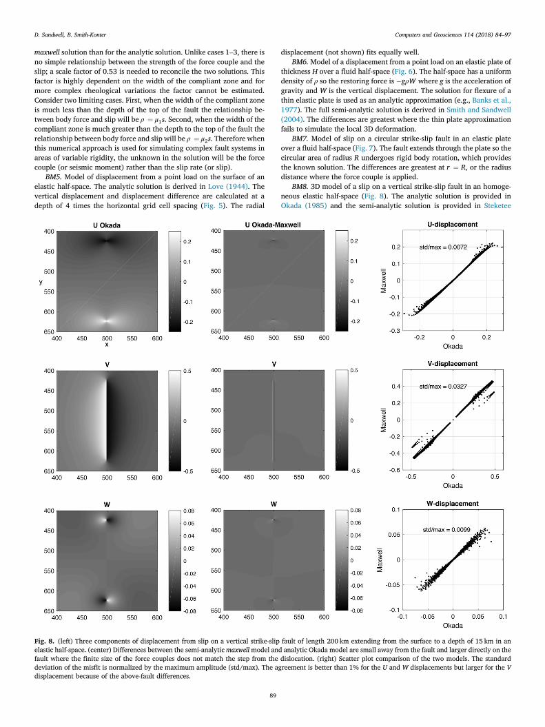
Fig. 8. (left) Three components of displacement from slip on a vertical strike-slipelastic half-space. (center) Differences between the semi-analytic maxwellmodel andfault where the finite size of the force couples does not match the step from thedeviation of the misfit is normalized by the maximum amplitude (std/max). The agdisplacement because of the above-fault differences.

89

displacement (not shown) fits equally well.BM6.Model of a displacement from a point load on an elastic plate of

thickness H over a fluid half-space (Fig. 6). The half-space has a uniformdensity of ρ so the restoring force is �gρW where g is the acceleration ofgravity and W is the vertical displacement. The solution for flexure of athin elastic plate is used as an analytic approximation (e.g., Banks et al.,1977). The full semi-analytic solution is derived in Smith and Sandwell(2004). The differences are greatest where the thin plate approximationfails to simulate the local 3D deformation.

BM7. Model of slip on a circular strike-slip fault in an elastic plateover a fluid half-space (Fig. 7). The fault extends through the plate so thecircular area of radius R undergoes rigid body rotation, which providesthe known solution. The differences are greatest at r ¼ R, or the radiusdistance where the force couple is applied.

BM8. 3D model of a slip on a vertical strike-slip fault in an homoge-neous elastic half-space (Fig. 8). The analytic solution is provided inOkada (1985) and the semi-analytic solution is provided in Steketee

fault of length 200 km extending from the surface to a depth of 15 km in ananalytic Okada model are small away from the fault and larger directly on thedislocation. (right) Scatter plot comparison of the two models. The standardreement is better than 1% for the U and W displacements but larger for the V

D. Sandwell, B. Smith-Konter Computers and Geosciences 114 (2018) 84–97

(1958) and implemented using grids of force couples in Smith andSandwell (2003). A 4096� 4096 computational array is used forcomputation, however only the local faulted region is shown inFigs. 8–11.

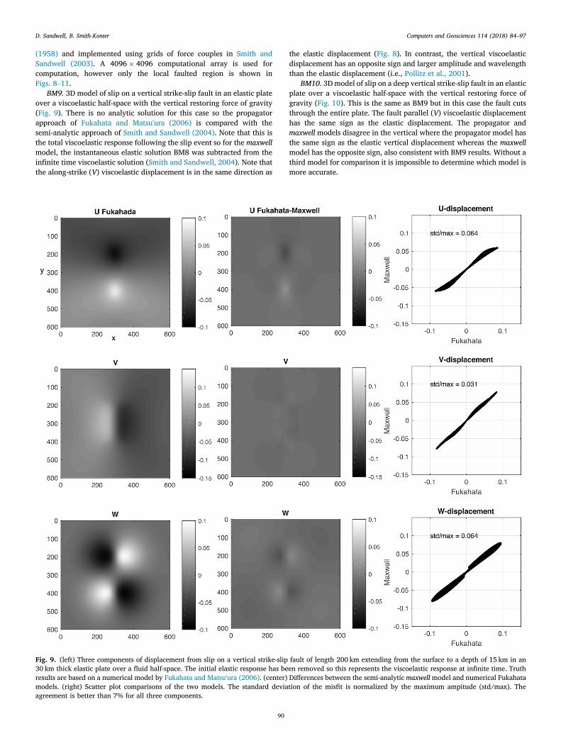
BM9. 3D model of slip on a vertical strike-slip fault in an elastic plateover a viscoelastic half-space with the vertical restoring force of gravity(Fig. 9). There is no analytic solution for this case so the propagatorapproach of Fukahata and Matsu'ura (2006) is compared with thesemi-analytic approach of Smith and Sandwell (2004). Note that this isthe total viscoelastic response following the slip event so for the maxwellmodel, the instantaneous elastic solution BM8 was subtracted from theinfinite time viscoelastic solution (Smith and Sandwell, 2004). Note thatthe along-strike (V) viscoelastic displacement is in the same direction as

Fig. 9. (left) Three components of displacement from slip on a vertical strike-slip30 km thick elastic plate over a fluid half-space. The initial elastic response has beresults are based on a numerical model by Fukahata and Matsu'ura (2006). (center)models. (right) Scatter plot comparisons of the two models. The standard deviaagreement is better than 7% for all three components.

90

the elastic displacement (Fig. 8). In contrast, the vertical viscoelasticdisplacement has an opposite sign and larger amplitude and wavelengththan the elastic displacement (i.e., Pollitz et al., 2001).

BM10. 3D model of slip on a deep vertical strike-slip fault in an elasticplate over a viscoelastic half-space with the vertical restoring force ofgravity (Fig. 10). This is the same as BM9 but in this case the fault cutsthrough the entire plate. The fault parallel (V) viscoelastic displacementhas the same sign as the elastic displacement. The propagator andmaxwell models disagree in the vertical where the propagator model hasthe same sign as the elastic vertical displacement whereas the maxwellmodel has the opposite sign, also consistent with BM9 results. Without athird model for comparison it is impossible to determine which model ismore accurate.

fault of length 200 km extending from the surface to a depth of 15 km in anen removed so this represents the viscoelastic response at infinite time. TruthDifferences between the semi-analytic maxwell model and numerical Fukahatation of the misfit is normalized by the maximum ampitude (std/max). The

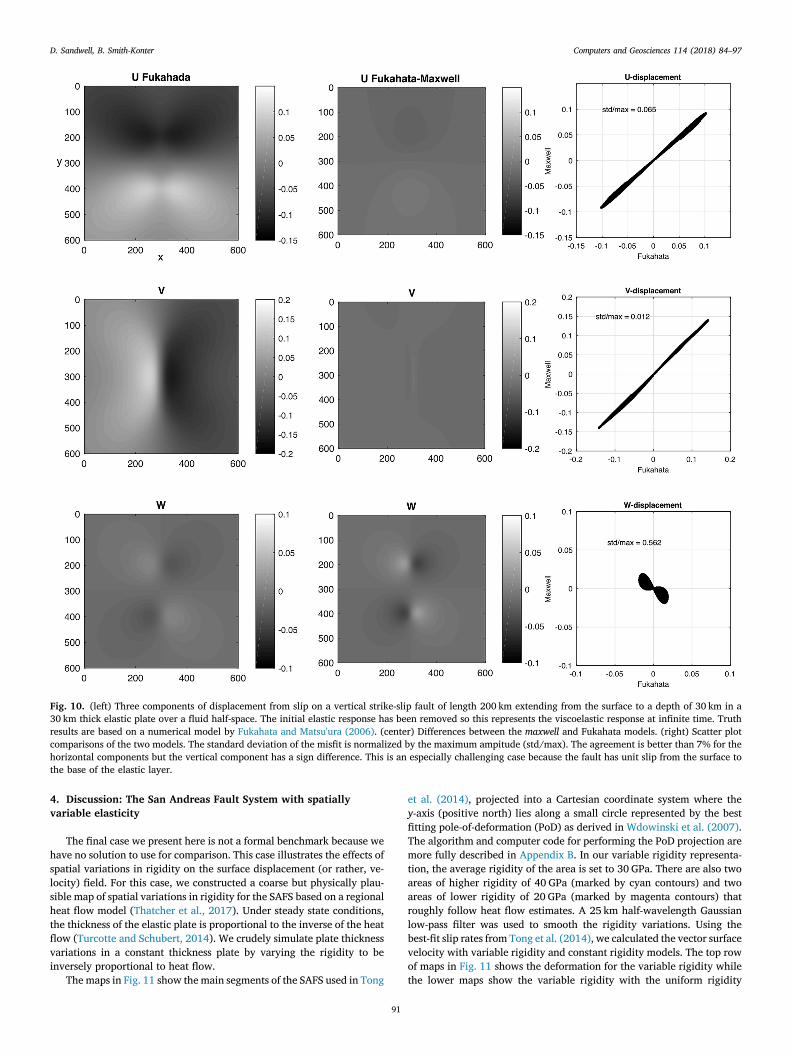
Fig. 10. (left) Three components of displacement from slip on a vertical strike-slip fault of length 200 km extending from the surface to a depth of 30 km in a30 km thick elastic plate over a fluid half-space. The initial elastic response has been removed so this represents the viscoelastic response at infinite time. Truthresults are based on a numerical model by Fukahata and Matsu'ura (2006). (center) Differences between the maxwell and Fukahata models. (right) Scatter plotcomparisons of the two models. The standard deviation of the misfit is normalized by the maximum ampitude (std/max). The agreement is better than 7% for thehorizontal components but the vertical component has a sign difference. This is an especially challenging case because the fault has unit slip from the surface tothe base of the elastic layer.

D. Sandwell, B. Smith-Konter Computers and Geosciences 114 (2018) 84–97

4. Discussion: The San Andreas Fault System with spatiallyvariable elasticity

The final case we present here is not a formal benchmark because wehave no solution to use for comparison. This case illustrates the effects ofspatial variations in rigidity on the surface displacement (or rather, ve-locity) field. For this case, we constructed a coarse but physically plau-sible map of spatial variations in rigidity for the SAFS based on a regionalheat flow model (Thatcher et al., 2017). Under steady state conditions,the thickness of the elastic plate is proportional to the inverse of the heatflow (Turcotte and Schubert, 2014). We crudely simulate plate thicknessvariations in a constant thickness plate by varying the rigidity to beinversely proportional to heat flow.

The maps in Fig. 11 show the main segments of the SAFS used in Tong

91

et al. (2014), projected into a Cartesian coordinate system where they-axis (positive north) lies along a small circle represented by the bestfitting pole-of-deformation (PoD) as derived in Wdowinski et al. (2007).The algorithm and computer code for performing the PoD projection aremore fully described in Appendix B. In our variable rigidity representa-tion, the average rigidity of the area is set to 30 GPa. There are also twoareas of higher rigidity of 40 GPa (marked by cyan contours) and twoareas of lower rigidity of 20 GPa (marked by magenta contours) thatroughly follow heat flow estimates. A 25 km half-wavelength Gaussianlow-pass filter was used to smooth the rigidity variations. Using thebest-fit slip rates from Tong et al. (2014), we calculated the vector surfacevelocity with variable rigidity and constant rigidity models. The top rowof maps in Fig. 11 shows the deformation for the variable rigidity whilethe lower maps show the variable rigidity with the uniform rigidity

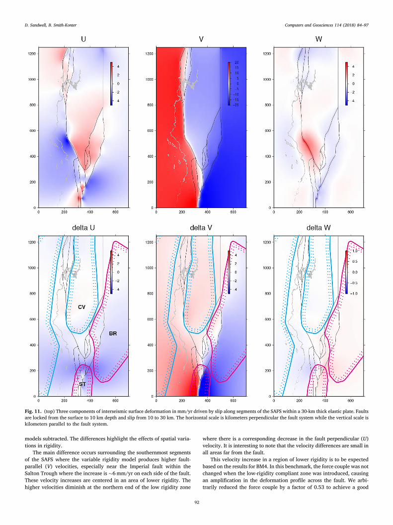
Fig. 11. (top) Three components of interseismic surface deformation in mm/yr driven by slip along segments of the SAFS within a 30-km thick elastic plate. Faultsare locked from the surface to 10 km depth and slip from 10 to 30 km. The horizontal scale is kilometers perpendicular the fault system while the vertical scale iskilometers parallel to the fault system.

D. Sandwell, B. Smith-Konter Computers and Geosciences 114 (2018) 84–97

models subtracted. The differences highlight the effects of spatial varia-tions in rigidity.

The main difference occurs surrounding the southernmost segmentsof the SAFS where the variable rigidity model produces higher fault-parallel (V) velocities, especially near the Imperial fault within theSalton Trough where the increase is �6mm/yr on each side of the fault.These velocity increases are centered in an area of lower rigidity. Thehigher velocities diminish at the northern end of the low rigidity zone

92

where there is a corresponding decrease in the fault perpendicular (U)velocity. It is interesting to note that the velocity differences are small inall areas far from the fault.

This velocity increase in a region of lower rigidity is to be expectedbased on the results for BM4. In this benchmark, the force couple was notchanged when the low-rigidity compliant zone was introduced, causingan amplification in the deformation profile across the fault. We arbi-trarily reduced the force couple by a factor of 0.53 to achieve a good

D. Sandwell, B. Smith-Konter Computers and Geosciences 114 (2018) 84–97

match. Similarly, the results shown in Fig. 11 would not match the GPSand InSAR data used by Tong et al. (2014) to constrain the slip rates.Therefore, after introducing lateral variations in rigidity, one must re-doa slip-rate inversion. The new unknowns will be moment rate rather thanslip rate as in the typical geodetic inversions. While geologists are moreinterested in slip rate for comparison with geological rates, moment rateis the most important parameter for earthquake hazard analysis (Fieldet al., 2014). One immediate implication for the Imperial fault is that ifthe region has relatively low rigidity, then the moment accumulation ratemust be smaller than has been estimated using a uniform rigidity model.This implies a lower seismic hazard in the region. The main objective ofthis model is to use lithospheric rheology models (Thatcher et al., 2017)to improve seismic hazard models.

5. Conclusions

We have added lateral variations in shear modulus to an existingcomputer code (maxwell) that is used for simulating time-dependentdeformation and stress in complex transform fault systems. The codewas tested using 8 analytic solutions for 2D and 3D cases. The morecomplex 3D viscoelastic response was validated through a comparisonwith published results based on a propagator matrix approach. Two of

93

the benchmarks included sharp step-like variations in shear modulus thatwere accurately modeled using the iterative spectral approach, although20 iterations were needed for convergence. The full San Andreas FaultSystem model needed only 4 iterations for convergence because thevariations in rigidity were smooth (�25 km) relative to the grid spacingof 1 km. The model uses force couples to simulate the faults that drive thedeformation. As expected, we find that a decrease in shear modulus in aregion surrounding a force couple results in an increase in deformation.Therefore geodetic inversions using this approach will need to solve formoment rate rather than slip rate. The maxwell computer code, as well asthe coordinate transformation code (trans_pole) and scripts needed toreproduce all the examples (Figs. 1–11), are available on GitHub.

Acknowledgements

We would like to thank Yukitoshi Fukahata for providing his nu-merical results for benchmarks 9 and 10. This work was partially fundedby the NASA Earth Surface and Interior Program (NNX16AK93G), NSF(EAR1614875 and EAR1147427). This research was also supported bythe Southern California Earthquake Center (Contribution No. 8007).SCEC is funded by NSF Cooperative Agreement EAR-1033462 and USGSCooperative Agreement G12AC20038.

Appendix A. MAXWELL: Description of the software installation, testing, and running benchmarks

This appendix describes themaxwell software distribution. The code is available online through GitHub and also as a single tar file. At the upper levelthere are 5 standard UNIX directories. After unpacking the tar file one should compile and test the code following the instructions provided in doc/README_compile_test_maxwell. You will need C and Fortran compilers. Also the reading and writing of grid files uses the GMT library. There are twoFORTRAN callable subroutines lib/readgrd.c and lib/writegrd.cwith versions for GMT5 and GMT4. You may need to modify all the makefiles to havethe correct paths to the GMT distribution. Also you could replace these routines with your favorite grid file format. The code should be tested using thetest examples in tests/test_maxwell_point. The tests compare the output with known solutions and report on any differences. After successfullyrunning the test exercise, one can reproduce all the benchmarks provided in this manuscript although Matlab and GMT5 will be needed to constructfigures.

Appendix B. TRANS_POLE: Scalar, vector, and tensor data projection

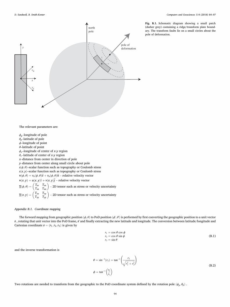
Our objectives are to project geospatial data from the standard latitude-longitude coordinate system to an approximate Cartesian coordinate systemwith the y-axis parallel to the relative plate motion and the x-axis perpendicular to the relative plate motion vector. These transformations are largelyprovided in Wdowinski (1998). This coordinate system is defined by the pole of deformation or PoD. The geometry is shown in Fig. B.1.

Computers and Geosciences 114 (2018) 84–97

D. Sandwell, B. Smith-Konter

94

Fig. B.1. Schematic diagram showing a small patch(darker grey) containing a ridge/transform plate bound-ary. The transform faults lie on a small circles about thepole of deformation.

The relevant parameters are:

ϕp–longitude of poleθp–latitude of poleϕ–longitude of pointθ–latitude of pointϕc–longitude of center of x-y regionθc–latitude of center of x-y regionx–distance from center in direction of poley–distance from center along small circle about polesðϕ;θÞ–scalar function such as topography or Coulomb stresssðx;yÞ–scalar function such as topography or Coulomb stressvðϕ; θÞ ¼ veðϕ; θÞbe þ vnðϕ; θÞbn – relative velocity vector

vðx; yÞ ¼ uðx; yÞbı þ vðx; yÞbj – relative velocity vector

Tðϕ; θÞ ¼�Tee TenTen Tnn

�– 2D tensor such as stress or velocity uncertainty

Tðx; yÞ ¼�Txx TxyTxy Tyy

�– 2D tensor such as stress or velocity uncertainty

Appendix B.1. Coordinate mapping

The forward mapping from geographic position ðϕ; θÞ to PoD position ðϕ'; θ'Þ is performed by first converting the geographic position to a unit vectorr , rotating that unit vector into the PoD frame, r' and finally extracting the new latitude and longitude. The conversion between latitude/longitude andCartesian coordinate r ¼ ðr1; r2; r3Þ is given by

r1 ¼ cos θ cos ϕr2 ¼ cos θ sin ϕr3 ¼ sin θ

(B.1)

and the inverse transformation is

θ ¼ sin�1ðr3Þ ¼ tan�1

r3ffiffiffiffiffiffiffiffiffiffiffiffiffiffi

r21 þ r22

q !

ϕ ¼ tan�1

�r2r1

� (B.2)

Two rotations are needed to transform from the geographic to the PoD coordinate system defined by the rotation pole ðϕp; θpÞ .

D. Sandwell, B. Smith-Konter Computers and Geosciences 114 (2018) 84–97

r' ¼ R2 θp � π2

R3��ϕp

�r (B.3)

� �

where

R2ðβÞ ¼0@ cos β 0 sin β

0 1 0�sin β 0 cos β

1A (B.4)

R3ðγÞ ¼0@ cos γ �sin γ 0

sin γ cos γ 00 0 1

1A (B.5)

Similarly if one were given the Cartesian coordinate in the PoD frame and wanted to convert back to the geographic frame then the following trans-formation would be used.

r ¼ R3�ϕp

�R2

�π2� θp

�r' (B.6)

One final issue is that we want to convert the position in the PoD frame to an SI distance unit relative to an origin. The approach would be to convert thecenter coordinate of the fault map to the PoD coordinates ðϕc;θcÞ→ðϕ'c;θ'cÞ. We can select any point for this, but a point somewhere in the center of themodel space is best. The x-y coordinates are

x ¼ Reðθ'c � θ'Þy ¼ Recosθ'cðϕ'c � ϕ'Þ:

(B.7)

Appendix B.2. Velocity vector rotation

When transforming a velocity vector field, one must rotate the east and north vector into the PoD frame. Again, a rotation matrix will be used forboth the forward the inverse transformations.

v'e

v'n

!¼ cos γ �sin γ

sin γ cos γ

! ve

vn

! ve

vn

!¼

cos γ sin γ

�sin γ cos γ

! v'e

v'n

! (B.8)

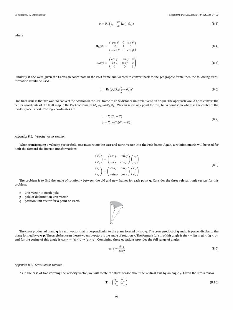
The problem is to find the angle of rotation γ between the old and new frames for each point q. Consider the three relevant unit vectors for thisproblem.

n – unit vector to north polep – pole of deformation unit vectorq – position unit vector for a point on Earth

The cross product of n and q is a unit vector that is perpendicular to th

e plane formed by n-o-q. The cross product of q and p is perpendicular to theplane formed by q-o-p. The angle between these two unit vectors is the angle of rotation γ. The formula for sin of this angle is sin γ ¼ jðn� qÞ � ðq� pÞjand for the cosine of this angle is cos γ ¼ ðn� qÞ � ðq� pÞ. Combining these equations provides the full range of angles

tan γ ¼ sin γcos γ

(B.9)

Appendix B.3. Stress tensor rotation

As in the case of transforming the velocity vector, we will rotate the stress tensor about the vertical axis by an angle γ. Given the stress tensor

T ¼�Txx Txy

Txy Tyy

�(B.10)

95

D. Sandwell, B. Smith-Konter Computers and Geosciences 114 (2018) 84–97

we would like to rotate it into a new primed system T' as given by the following equation

T' ¼ RTRT (B.11)

where the rotation matrix is given by

R ¼�cos γ �sin γsin γ cos γ

�(B.12)

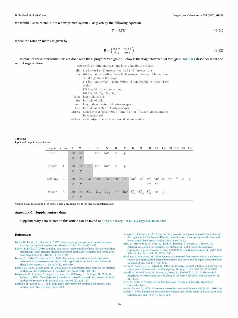
In practice these transformations are done with the C-program trans_pole.c. Below is the usage statement of trans_pole. Table B.1 describes input andoutput organization.

Table B.1Input and output data columns.

Shaded boxes are required for input. x and y are input fields for inverse transformation.

Appendix C. Supplementary data

Supplementary data related to this article can be found at https://doi.org/10.1016/j.cageo.2018.01.009.

References

Banks, R., Parker, R., Huestis, S., 1977. Isostatic compensation on a continental scale:local versus regional mechanisms. Geophys. J. Int. 51 (2), 431–452.

Barbot, S., Fialko, Y., 2010. A unified continuum representation of post-seismic relaxationmechanisms: semi-analytic models of afterslip, poroelastic rebound and viscoelasticflow. Geophys. J. Int. 182 (3), 1124–1140.

Barbot, S., Fialko, Y., Sandwell, D., 2009. Three-dimensional models of elastostaticdeformation in heterogeneous media, with applications to the Eastern CaliforniaShear Zone. Geophys. J. Int. 179 (1), 500–520.

Barbot, S., Fialko, Y., Sandwell, D., 2008. Effect of a compliant fault zone on the inferredearthquake slip distribution. J. Geophys. Res. Solid Earth 113 (B6).

Bürgmann, R., Ergintav, S., Segall, P., Hearn, E., McClusky, S., Reilinger, R., With, H.,Zschau, J., 2002. Time-dependent distributed afterslip on and deep below the Izmitearthquake rupture. Bull. Seismol. Soc. Am. 92 (1), 126–137.

Burridge, R., Knopoff, L., 1964. Body force equivalents for seismic dislocations. Bull.Seismol. Soc. Am. 54 (6A), 1875–1888.

96

Chuang, R., Johnson, K., 2011. Reconciling geologic and geodetic model fault slip-ratediscrepancies in Southern California: consideration of nonsteady mantle flow andlower crustal fault creep. Geology 39 (7), 627–630.

Field, E., Arrowsmith, R., Biasi, G., Bird, P., Dawson, T., Felzer, K., Jackson, D.,Johnson, K., Jordan, T., Madden, C., Michael, A., 2014. Uniform Californiaearthquake rupture forecast, version 3 (UCERF3)–the time-independent model. Bull.Seismol. Soc. Am. 104 (3), 1122–1180.

Fukahata, Y., Matsu'ura, M., 2006. Quasi-static internal deformation due to a dislocationsource in a multilayered elastic/viscoelastic half-space and an equivalence theorem.Geophys. J. Int. 166 (1), 418–434.

Garcia, E., Sandwell, D., Luttrell, K., 2014. An iterative spectral solution method for thinelastic plate flexure with variable rigidity. Geophys. J. Int. 200 (2), 1012–1028.

Howell, S., Smith-Konter, B., Frazer, N., Tong, X., Sandwell, D., 2016. The verticalfingerprint of earthquake cycle loading in southern California. Nat. Geosci. 9 (8),611–614.

Love, A., 1944. A Treatise on the Mathematical Theory of Elasticity. CambridgeUniversity Press.

Nur, A., Mavko, G., 1974. Postseismic viscoelastic rebound. Science 183 (4121), 204–206.Okada, Y., 1985. Surface deformation due to shear and tensile faults in a half-space. Bull.

Seismol. Soc. Am. 75 (4), 1135–1154.

D. Sandwell, B. Smith-Konter Computers and Geosciences 114 (2018) 84–97

Pollitz, F., 1997. Gravitational viscoelastic postseismic relaxation on a layered sphericalEarth. J. Geophys. Res. Solid Earth 102 (B8), 17921–17941.

Pollitz, F., Wicks, C., Thatcher, W., 2001. Mantle flow beneath a continental strike-slipfault: postseismic deformation after the 1999 Hector Mine earthquake. Science 293(5536), 1814–1818.

Rundle, J., Jackson, D., 1977. A three-dimensional viscoelastic model of a strike slip fault.Geophys. J. Int. 49 (3), 575–591.

Rybicki, K., 1971. The elastic residual field of a very long strike-slip fault in the presenceof a discontinuity. Bull. Seismol. Soc. Am. 61 (1), 79–92.

Sandwell, D., 1984. Thermomechanical evolution of oceanic fracture zones. J. Geophys.Res. Solid Earth 89 (B13), 11401–11413.

Segall, P., 2010. Earthquake and Volcano Deformation. Princeton University Press.Simons, M., Fialko, Y., Rivera, L., 2002. Coseismic deformation from the 1999 Mw 7.1

Hector Mine, California, earthquake as inferred from InSAR and GPS observations.Bull. Seismol. Soc. Am. 92 (4), 1390–1402.

Smith, B., Sandwell, D., 2006. A model of the earthquake cycle along the San Andreasfault System for the past 1000 years. J. Geophys. Res. Solid Earth 111 (B1),1405–1425.

Smith, B., Sandwell, D., 2004. A three-dimensional semianalytic viscoelastic model fortime-dependent analyses of the earthquake cycle. J. Geophys. Res. Solid Earth 109(B12), 12401–12427.

Smith, B., Sandwell, D., 2003. Coulomb stress accumulation along the San Andreas faultsystem. J. Geophys. Res. Solid Earth 108 (B6), 2296–2313.

97

Smith-Konter, B., Sandwell, D., 2009. Stress evolution of the San Andreas Fault system:recurrence interval versus locking depth. Geophys. Res. Lett. 36, 13304–13309.https://doi.org/10.1029/2009GL037235.

Steketee, J., 1958. On Volterra's dislocations in a semi-infinite elastic medium. Can. J.Phys. 36 (2), 192–205.

Takeuchi, C., Fialko, Y., 2013. On the effects of thermally weakened ductile shear zoneson postseismic deformation. J. Geophys. Res. Solid Earth 118 (12), 6295–6310.

Thatcher, W., 1983. Nonlinear strain buildup and the earthquake cycle on the SanAndreas fault. J. Geophys. Res. Solid Earth 88 (B7), 5893–5902.

Thatcher, W., Chapman, D., Allam, A., 2017. Refining Southern California geothermsusing seismologic, geologic, and petrologic constraints. In: Annual Meeting of theSouthern California Earthquake Center p. poster 224, august 15, 2017.

Tong, X., Smith-Konter, B., Sandwell, D., 2014. Is there a discrepancy between geologicaland geodetic slip rates along the San Andreas Fault system? J. Geophys. Res. SolidEarth 119 (3), 2518–2538.

Turcotte, D., Schubert, G., 2014. Geodynamics. Cambridge University Press.Wdowinski, S., 1998. A theory of intraplate tectonics. J. Geophys. Res. Solid Earth 103

(B2), 5037–5059.Wdowinski, S., Smith-Konter, B., Sandwell, D., 2007. Diffuse interseismic deformation

across the Pacific-North America plate boundary. Geology 35 (4), 311–314.Weertman, J., 1964. Continuum distribution of dislocations on faults with finite friction.

Bull. Seismol. Soc. Am. 54 (4), 1035–1058.