MCPLOTS: a particle physics resource based on volunteer computing

Eur. Phys. J. C (2014) 74:2714DOI 10.1140/epjc/s10052-014-2714-9

Special Article - Tools for Experiment and Theory

MCPLOTS: a particle physics resource based on volunteercomputing

A. Karneyeu1, L. Mijovic2,3, S. Prestel2,4, P. Z. Skands5,a

1 Institute for Nuclear Research, Moscow, Russia2 Deutsches Elektronen-Synchrotron, DESY, 22603 Hamburg, Germany3 Irfu/SPP, CEA-Saclay, bat 141, 91191 Gif-sur-Yvette Cedex, France4 Department of Astronomy and Theoretical Physics, Lund University, Lund, Sweden5 European Organization for Nuclear Research, CERN, 1211 Geneva 23, Switzerland

Received: 1 July 2013 / Accepted: 3 January 2014 / Published online: 5 February 2014© The Author(s) 2014. This article is published with open access at Springerlink.com

Abstract The mcplots.cern.ch web site (mcplots) pro-vides a simple online repository of plots made with high-energy-physics event generators, comparing them to a widevariety of experimental data. The repository is based on thehepdata online database of experimental results and on therivet Monte Carlo analysis tool. The repository is contin-ually updated and relies on computing power donated byvolunteers, via the lhc@home 2.0 platform.

1 Introduction

Computer simulations of high-energy interactions are usedto provide an explicit theoretical reference for a wide rangeof particle-physics measurements. In particular, Monte Carlo(MC) event generators [1–3] enable a comparison betweentheory and experimental data down to the level of individualparticles. An exact calculation taking all relevant dynamicsinto account would require a solution to infinite-order per-turbation theory coupled to non-perturbative QCD—a long-standing and unsolved problem. In the absence of such asolution, MC generators apply a divide-and-conquer strat-egy, factorizing the problem into many simpler pieces, andtreating each one at a level of approximation dictated by ourunderstanding of the corresponding parts of the underlyingfundamental theory.

A central question, when a disagreement is found betweensimulation and data, is thus whether the discrepancy is withinthe intrinsic uncertainty allowed by the inaccuracy of the cal-culation, or not. This accuracy depends both on the sophisti-cation of the simulation itself, driven by the development andimplementation of new theoretical ideas, but it also dependscrucially on the available constraints on the free parameters of

a e-mail: [email protected]

the model. Using existing data to constrain these is referredto as “tuning”. Useful discussions of tuning can be found,e.g., in [1,2,4–10].

Typically, experimental studies include comparisons ofspecific models and tunes to the data in their publications.Such comparisons are useful both as immediate tests of com-monly used models, and to illustrate the current amount oftheoretical uncertainty surrounding a particular distribution.They also provide a set of well-defined theoretical referencecurves that can be useful as benchmarks for future stud-ies. However, many physics distributions, in particular thosethat are infrared (IR) sensitive1 often represent a compli-cated cocktail of physics effects. The conclusions that canbe drawn from comparisons on individual distributions aretherefore limited. They also gradually become outdated, asnew models and tunes supersede the old ones. In the longterm, the real aim is not to study one distribution in detail,for which a simple fit would in principle suffice, but to studythe degree of simultaneous agreement or disagreement overmany, mutually complementary, distributions. This is also aprerequisite to extend the concept of tuning to more rigor-ous consistency tests of the underlying physics model, forinstance as proposed in [8].

The effort involved in making simultaneous comparisonsto large numbers of experimental distributions, and to keepthose up to date, previously meant that this kind of exercisewas restricted to a small set of people, mostly Monte Carloauthors and dedicated experimental tuning groups. The aimwith the mcplots.cern.ch (mcplots) web site is to provide a

1 IR sensitive observables change value when adding an infinitely softparticle or when splitting an existing particle into two collinear ones.Such variables have larger sensitivity to non-perturbative physics thanIR safe ones, see, e.g., [2,11]. Note also that we here use the word “IR”as a catchall for both the soft and collinear limits.

123

2714 Page 2 of 22 Eur. Phys. J. C (2014) 74:2714

simple browsable repository of such comparisons so that any-one can quickly get an idea of how well a particular modeldescribes various data sets.2 Simultaneously, we also aimto make all generated data, parameter cards, source codes,experimental references, etc, freely and directly available inas useful forms as possible, for anyone who wishes to repro-duce, re-plot, or otherwise make use of the results and toolsthat we have developed.

The mcplots web site is now at a mature and stable stage.It has been online since Dec 2010 and is nearing a trilliongenerated events in total (900 billion as of June 2013). Thispaper is intended to give an overview of what is availableon the site, and how to use it. In particular, Sect. 2 con-tains a brief “user guide” for the site, explaining its featuresand contents in simple terms, how to navigate through thesite, and how to extract plots and information about howthey were made from it. As a reference for further additionsand updates, and for the benefit of future developers, Sects.3–7 then describe the more concrete details of the technicalstructure and implementation of the site, which the ordinaryuser would not need to be familiar with.

Section 3 describes the architecture of the site, and thethinking behind it. It currently relies on the following basicprerequisites,

• The hepdata database [13] of experimental results.• The rivet Monte Carlo analysis tool [14] which contains

a large code library for comparing the output of MC gen-erators to distributions from hepdata. rivet in turn relieson the hepmc universal event-record format [15], on thefastjet package for jet clustering [16,17], and on thelhapdf library for parton densities [18,19].

• Monte Carlo event generators. Currently implementedgenerators include alpgen [20], epos [21] herwig++[22], phojet [23], pythia 6 [24], pythia 8 [25], sherpa[26], and vincia [27]. Some of these in turn use theLes Houches Event File (LHEF) format [28,29] to passparton-level information back and forth.

• The lhc@home 2.0 framework for volunteer cloud com-puting [30–33]. lhc@home 2.0 in turn relies on cernvm[34,35] (a Virtual-Machine computing environment basedon Scientific Linux), on the copilot job submission sys-tem [36,35], and on the Boinc middleware for volunteercomputing [37,38].

The basic procedure to include a new measurement onmcplots is, first, to provide the relevant experimental datapoints to hepdata, second to provide a rivet routine for thecorresponding analysis, and lastly to provide a very small

2 Note: this idea was first raised in the now defunct jetweb project[12]. The CERN Generator Services (GENSER) project also maintainsa set of web pages with basic generator validation plots/calculations.

additional amount of information to mcplots, essentiallyspecifying the placement of the observable in the mcplotsmenus and summarizing the cuts applied in a LaTeX string, ase.g. exemplified by the already existing analyses on the site.This is described in more detail in Sect. 4.

To update mcplots with a new version of an existing gen-erator, the first step is to check whether it is already avail-able in the standard CERN Generator Services (GENSER)repository [39], and if not announce the new version to theGENSER team. The mcplots steering scripts should thenbe updated to run jobs for the new version, as described inSect. 5.

To add a new generator to mcplots, the first step is tocheck that it can run within cernvm. cernvm provides astandardized Scientific-Linux environment that should beappropriate for most high-energy physics (HEP) applica-tions, including several commonly used auxiliary packagessuch as the GNU Scientific Library (GSL), the C++ BOOSTlibraries, and many others. A standalone version of cernvmcan be downloaded from [34] for testing purposes. To theextent that dependencies require additional packages to beinstalled, these should be communicated to the mcplotsand cernvm development teams. The code should then beprovided to the GENSER team for inclusion in the stan-dard CERN generator repository. The complete procedureis described in more detail in Sect. 6.

The main benefit of using cernvm is that this has enabledmcplots to draw on significant computing resources madeavailable by volunteers, via the Boinc and lhc@home 2.0projects. Through the intermediary of cernvm, generatorauthors can concentrate on developing code that is com-patible with the Scientific Linux operating system, a fairlystandard environment in our field. This code can then berun on essentially any user platform by encapsulating itwithin cernvm and distributing it via the Boinc middle-ware. (The latter also enabled us to access a large exist-ing Boinc volunteer-computing community.) The resulting“test4theory” project [33,40] was the first applicationdeveloped for the lhc@home 2.0 framework, see [30,33],and it represents the world’s first virtualization-based volun-teer cloud. A brief summary of it is given in Sect. 7.

2 User guide

In this section, we describe the graphical interface on themcplots web site and how to navigate through it. Care hasbeen taken to design it so as to make all content accessiblethrough a few clicks, in a hopefully intuitive manner.

2.1 The main menu

The main menu, shown in Fig. 1, is always located at thetop left-hand corner of the page. The Front Page link is just

123

Eur. Phys. J. C (2014) 74:2714 Page 3 of 22 2714

Fig. 1 The main mcplots menu

a “home” button that takes you back to the starting pagefor mcplots, and the LHC@home 2.0 one takes you to theexternal lhc@home 2.0 web pages, where you can connectyour computer to the volunteer cloud that generates eventsfor mcplots.

The Generator Versions link opens a configuration pagethat allows you to select which generator versions you wantto see results for on the site. The default is simply to usethe most recently implemented ones, but if your analysis, forinstance, uses an older version of a particular generator, youcan select among any of the previously implemented versionson the site by choosing that specific version on the GeneratorVersions page. All displayed content on the site will thereafterreflect your choice, as you can verify by checking the explicitversion numbers written at the bottom of each plot. You canreturn to the Generator Versions page at any time to modifyyour choice. After making your choice, click on the FrontPage button to exit the Generator Versions view.

The Generator Validation link changes the page layout andcontent from the Front Page one, to one in which differentgenerator versions can be compared both globally, via χ2

values, and individually on each distribution. This view willbe discussed in more detail in Sect. 2.4.

The Update History link simply takes you to a page onwhich you can see what the most recent changes and additionsto the site were, and its previous history.

As an experimental social feature, we have added a “like”button to the bottom of the front page, which you can use toexpress if you are happy with the mcplots site.

2.2 The analysis filter

Immediately below the main menu, we have collected a fewoptions to control and organize which analyses you wantto see displayed on the site, under the subheading AnalysisFilter, illustrated in Fig. 2.

At the time of writing, the main choice you have hereis between ALL pp/ppbar (for hadron collisions) and ALLee (for fragmentation in electron-positron collisions). Thedefault is ALL pp/ppbar, so if you are interested in seeingall hadron-collider analyses, you will not have to make anychanges here. Using the Specific Analysis dropdown menu,you can also select to see only the plots from one partic-ular rivet analysis. The latter currently requires that youknow the rivet ID of the analysis you are interested in.The ID is typically formed from the experiment name, theyear, and the inSPIRE ID (or SPIRES ID, for older analy-ses) of the paper containing the original analysis, as illus-trated in Fig. 2 (the numbers beginning with “I” are inSPIREcodes, while ones beginning with “S” are SPIRES ones).You can also find this information in the rivet user man-ual [14] and/or on the http://rivet.hepforge.org/ rivet webpages.

Finally, if you click on Latest Analyses, only those anal-yses that were added in the last update of the site will beshown. This can be useful to get a quick overview of what isnew on the site, for instance to check for new distributionsthat are relevant to you and that you may not have been ableto see on your last visit to the site. More options may ofcourse be added in the future, in particular as the number ofobservables added to the pp/ppbar set grows.

2.3 Selecting observables

Below the Analysis Filter, the list of processes and observ-ables for the selected set of analyses is shown. This is illus-trated in Fig. 3.

Clicking on any blue link below one of the process headers(e.g. below the “Jets” header), Fig. 3, or any blue link in theshaded drop-down menus, Fig. 3, will open the plot page forthat observable in the right-hand part of the page.

Fig. 2 The analysis filtersubmenu; normal view (left) andafter clicking on the SpecificAnalysis dropdown menu(right)

(a) Analysis Filter: Normal View (b) Analysis Filter: Dropdown Menu

123

http://rivet.hepforge.org/


Fig. 3 Illustrations of theprocess and observables list;normal view (left) and afterclicking on a shaded dropdownmenu (right), in this caseIdentified Particles: Y

(a) The Process and Observables List (b) An expanded dropdown menu

Fig. 4 The plot page. The generator and tune group selections are at the top, followed by the available plots for the chosen observable, ordered byCM energy and subordered alphabetically

At the top of the plot page, Fig. 4, you can select whichgenerators and tune combinations you want to see on thepage. By default, you are shown the results obtained withdefault settings of the available generators, but the links foreach generator give you access to see results for differenttune and model variations. Use the Custom link to specifyyour own set of generators and tunes. The available plots forthe chosen settings are shown starting with the highest CMenergies at the top of the page, and, for each CM energy,cascading from left to right alphabetically.

For many observables, measurements have been madeusing a variety of different cuts and triggers. These are indi-cated both above the plots and on the plots themselves, so asto minimize the potential for misinterpretation. In the exam-

ple of charged-particle multiplicity distributions shown inFig. 4, the two first plots that appear are thus ALICE (left),for their INEL > 0 cuts [41], and ATLAS (right), using theirNch ≥ 1 and pT > 2.5 GeV cuts [42]. We explain how to findthe correct references and run cards for each plot and gener-ator below. Note that, for the Monte Carlo runs, the numberof events in the smallest sample is shown along the right-hand edge of each plot. I.e., if two generators were used, andthe statistics were N1 and N2 events, respectively, the valueprinted is min(N1, N2).

Underneath each plot is shown a ratio pane, showing thesame results normalized to the data (or to the first MC curveif there are no data points on the plot). This is illustrated inFig. 5.

123


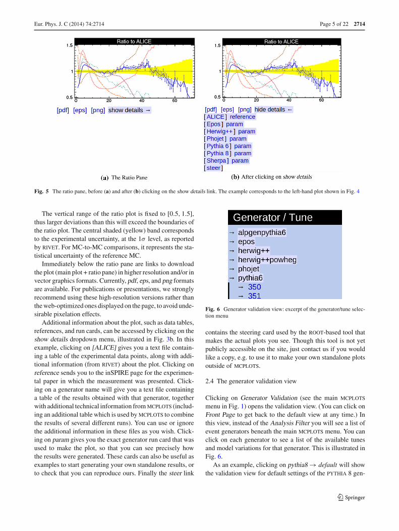
Fig. 5 The ratio pane, before (a) and after (b) clicking on the show details link. The example corresponds to the left-hand plot shown in Fig. 4

The vertical range of the ratio plot is fixed to [0.5, 1.5],thus larger deviations than this will exceed the boundaries ofthe ratio plot. The central shaded (yellow) band correspondsto the experimental uncertainty, at the 1σ level, as reportedby rivet. For MC-to-MC comparisons, it represents the sta-tistical uncertainty of the reference MC.

Immediately below the ratio pane are links to downloadthe plot (main plot + ratio pane) in higher resolution and/or invector graphics formats. Currently, pdf, eps, and png formatsare available. For publications or presentations, we stronglyrecommend using these high-resolution versions rather thanthe web-optimized ones displayed on the page, to avoid unde-sirable pixelation effects.

Additional information about the plot, such as data tables,references, and run cards, can be accessed by clicking on theshow details dropdown menu, illustrated in Fig. 3b. In thisexample, clicking on [ALICE] gives you a text file contain-ing a table of the experimental data points, along with addi-tional information (from rivet) about the plot. Clicking onreference sends you to the inSPIRE page for the experimen-tal paper in which the measurement was presented. Click-ing on a generator name will give you a text file containinga table of the results obtained with that generator, togetherwith additional technical information from mcplots (includ-ing an additional table which is used by mcplots to combinethe results of several different runs). You can use or ignorethe additional information in these files as you wish. Click-ing on param gives you the exact generator run card that wasused to make the plot, so that you can see precisely howthe results were generated. These cards can also be useful asexamples to start generating your own standalone results, orto check that you can reproduce ours. Finally the steer link

Fig. 6 Generator validation view: excerpt of the generator/tune selec-tion menu

contains the steering card used by the root-based tool thatmakes the actual plots you see. Though this tool is not yetpublicly accessible on the site, just contact us if you wouldlike a copy, e.g. to use it to make your own standalone plotsoutside of mcplots.

2.4 The generator validation view

Clicking on Generator Validation (see the main mcplotsmenu in Fig. 1) opens the validation view. (You can click onFront Page to get back to the default view at any time.) Inthis view, instead of the Analysis Filter you will see a list ofevent generators beneath the main mcplots menu. You canclick on each generator to see a list of the available tunesand model variations for that generator. This is illustrated inFig. 6.

As an example, clicking on pythia8 → default will showthe validation view for default settings of the pythia 8 gen-

123


Fig. 7 Generator validation:example showing (an excerpt of)the validation view for defaultsettings of the pythia 8generator

erator, in the right-hand side of the page, illustrated in Fig. 7.In this view, no plots are shown immediately. Instead you arepresented with a table of 〈χ2〉 values, averaged over all mea-surements within each process category. Note that we use aslightly modified definition of 〈χ2〉,

〈χ2〉mcplots = 1

Nbins

Nbins∑

i=1

(MCi − Datai )2

σ 2Data,i + σ 2

MC,i + (εMCMCi )2,

(1)

where σData,i is the uncertainty on the experimental measure-ment (combined statistical and systematic) of bin number i ,and σMC,i is the (purely statistical) MC uncertainty in thesame bin. The additional relative uncertainty, εMC, associ-ated with the MC prediction, is commented on below. Fromthe MC and data histograms alone, it is difficult to determineunambiguously whether the number of degrees of freedomfor a given distribution is Nbins or (Nbins − 1), hence we cur-rently use 1/Nbins as the normalization factor for all 〈χ2〉calculations.

At the top of the page, you can select which versions of thegenerator you want to include in the table. Click the Displaybutton to refresh the table after making modifications.

Below the line labelled Process Summary, we show themain table of 〈χ2〉 values for the versions you have selected,as well as the relative changes between successive ver-sions, thus allowing you to look for any significant changesthat may have resulted from improvements in the mod-elling/tuning (reflected by decreasing χ2 values) or mistun-ings/bugs (reflected by increasing χ2 values). The largestand smallest individual 〈χ2〉 values (and changes) in the rel-evant data set are also shown, in smaller fonts, above andbelow the average values. To aid the eye, values smaller than1 are shaded green (corresponding to less than 1σ averagedeviation from the data), values between 1 and 4 are shadedorange (corresponding to less than 2σ deviation), and values

greater than 4 are shaded red, following the spirit of the LesHouches “tune killing” exercise reported on in [10]. In theexample shown in Fig. 7, the changes are less than a few percent, indicative of no significant overall change.

Bear in mind that the statistical precision of the MC sam-ples plays a role, hence small fluctuations in these numbersare to be expected, depending on the available numbers ofgenerated events for each version. A future revision thatcould be considered would be to reinterpret the statisticalMC uncertainties in terms of uncertainties on the calculated〈χ2〉 values themselves. This would allow a better distinctionbetween a truly good description (low 〈χ2〉 with small uncer-tainty) and artificially low 〈χ2〉 values caused by low MCstatistics (low 〈χ2〉 with large uncertainty). Such improve-ments would certainly be mandatory before making any rig-orous conclusions using this tool, as well as for objectiveinterpretations of direct comparisons between different gen-erators. For the time being, the tool is not intended to providesuch quantitative discriminations, but merely to aid authorsin making a qualitative assessment of where their codes andtunes work well, and where there are problems.

Note: to make these numbers more physically meaning-ful, the generator predictions are assigned a flat εMC = 5 %“theory uncertainty” in addition to the purely statistical MCuncertainty, see equation (1), as a baseline sanity limit for theachievable theoretical accuracy with present-day models. Afew clear cases of GIGO3 are excluded from the χ2 calcu-lation, but some problematic cases remain. Thus, e.g., if acalculation returns a too small cross section for a dimension-ful quantity, the corresponding χ2 value will be large, eventhough the shape of the distribution may be well described. Itcould be argued how this should be treated, how much uncer-tainty should be allowed for each observable, how to compareconsistently across models/tunes with different numbers ofgenerated events, whether it is reasonable to include observ-

3 Garbage In, Garbage Out.

123


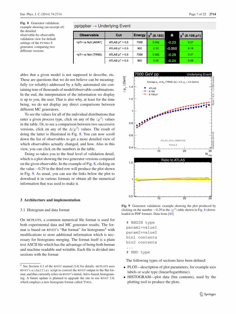
Fig. 8 Generator validation:example showing (an excerpt of)the detailedobservable-by-observablevalidation view for defaultsettings of the pythia 8generator, comparing twodifferent versions

ables that a given model is not supposed to describe, etc.These are questions that we do not believe can be meaning-fully (or reliably) addressed by a fully automated site con-taining tens of thousands of model/observable combinations.In the end, the interpretation of the information we displayis up to you, the user. That is also why, at least for the timebeing, we do not display any direct comparisons betweendifferent MC generators.

To see the values for all of the individual distributions thatenter a given process type, click on any of the 〈χ2〉 valuesin the table. Or, to see a comparison between two successiveversions, click on any of the �〈χ2〉 values. The result ofdoing the latter is illustrated in Fig. 8. You can now scrolldown the list of observables to get a more detailed view ofwhich observables actually changed, and how. Also in thisview, you can click on the numbers in the table.

Doing so takes you to the final level of validation detail,which is a plot showing the two generator versions comparedon the given observable. In the example of Fig. 8, clicking onthe value −0.29 in the third row will produce the plot shownin Fig. 9. As usual, you can use the links below the plot todownload it in various formats or obtain all the numericalinformation that was used to make it.

3 Architecture and implementation

3.1 Histogram and data format

On mcplots, a common numerical file format is used forboth experimental data and MC generator results. The for-mat is based on rivet’s “flat format” for histograms4 withmodifications to store additional information which is nec-essary for histograms merging. The format itself is a plaintext ASCII file which has the advantage of being both humanand machine readable and writable. Each file is divided intosections with the format

4 See Section 4.1 of the rivet manual [14] for details. mcplots usesrivet’s aida2flat script to convert the rivet-output to the flat for-mat, and thus currently relies on rivet’s initial, Aida-based, histogram-ing. A future update is planned to upgrade the site to use rivet 2.0,which employs a new histogram format called Yoda.

chgN10 20 30

[GeV

]⟩

T p⟨

0.4

0.6

0.8

1

1.2

1.4ATLAS8.1658.108.p1

7000 GeV pp Underlying Event

mcp

lots

.cer

n.ch

2.2

M e

vent

s≥

Riv

et 1

.8.2

,

Pythia 8

ATLAS_2010_S8894728

> 0.5 GeV/c)T

| < 2.5, pη (TRNS) (|ch vs NT

Average p

10 20 300.5

1

1.5Ratio to ATLAS

Fig. 9 Generator validation: example showing the plot produced byclicking on the number −0.29 in the 〈χ2〉 table shown in Fig. 8 (down-loaded in PDF format). Data from [43]

# BEGIN typeparam1=value1param2=value2bin1 contentsbin2 contents...# END type

The following types of sections have been defined:

• PLOT—description of plot parameters, for example axislabels or scale type (linear/logarithmic).

• HISTOGRAM—plot data (bin contents), used by theplotting tool to produce the plots.

123


• HISTOSTATS, PROFILESTATS—additional histogram(or profile) statistical data, used to merge histograms fromdifferent subruns.

• METADATA—description of MC generator parameters,for example generator name and version, simulated pro-cess and cross section, etc.

Section contents can be of two kinds: parameter value def-initions or bin value definitions. Parameter value definitionshave the same format for all types of sections. Bin value defi-

nitions contain several values on each line, e.g. describing thebin position, contents, and uncertainties, with the followingspecific formats for each section type:

HISTOGRAM:xLo xMid xHi yValue error- error+

HISTOSTATS:xLo xMid xHi entries sumW sumW2 sumXW sumX2W

PROFILESTATS:xLo xMid xHi entries sumW sumW2 sumXW sumX2W sumYW sumY2W sumY2W2

where:

• xLo, xHi—bin edges low and high positions.• xMid—bin centre position.• yValue—bin value.• error−, error+ —bin negative and positive errors.• entries—number of bin fills.• sum*—sums of various quantities accumulated during

bin fills: weight, weight*weight, X*weight, X*X*weight,Y*weight, Y*Y*weight, Y*Y*weight*weight.

As mentioned above, the sum-type quantities provide theadditional statistical information needed to combine his-tograms from different runs.

3.2 Directory structure

mcplots is structured as a directory tree, with separate subdi-rectories for different purposes (WWW content, MC produc-tion scripts, documentation, …). In the following, we assumethat this directory structure has been installed in a globalhome directory, which we call

$HOME = /home/mcplots # MCPLOTS home directory

The location /home/mcplots corresponds to the currentimplementation on the mcplots.cern.ch server. There are fiveimportant subdirectories in the home directory:

$DOC = $HOME/doc # Documentation and Help$PLOTTER = $HOME/plotter # Source code for ROOT-based plotting tool$POOL = $HOME/pool # Output from BOINC cluster$RELEASE = $HOME/release # Collection of generated (MC) data$SCRIPTS = $HOME/scripts # Production and update scripts$WWW = $HOME/www # Front of house: WWW pages and content

The $DOC directory contains documentation and help con-tent that extends and updates this write-up and should be

consulted by future developers. The $PLOTTER directory con-tains the C++ source code and Makefile for the small plottingutility used to generate the plots on the mcplots web pages.It only depends on ROOT and takes histogram/data files inthe format used on the mcplots site as input. It can be copiedand/or modified for personal use, if desired, as e.g., in [44].Any changes to the code located in the $PLOTTER directoryitself, on the mcplots server, will be reflected in the plotsappearing on the site, after the plotter has been recompiledand the browser cache is refreshed.

The $POOL directory contains the MC data sets generatedby the Test4Theory Boinc cluster.

The $RELEASE directory contains MC data sets generatedmanually and combinations of data sets (so-called releases).

123


For example typically the data visible on the public sitemcplots.cern.ch is a combination of Boinc data sets (whichhave large statistics) and a number of manually generateddata sets applied on top, for distributions that cannot be run onthe Boinc infrastructure, or to add new versions of generatorswhich were not yet available at the time of generation of theBoinc data set.

The $SCRIPTS directory contains various scripts used toorganize and run generator jobs, and to update the contentsof the $WWW directory which contains all the HTML and PHPsource code, together with style and configuration files, forthe mcplots.cern.ch front end of the site.

This directory structure is clearly visible in the mcplotsSVN repository, which is located at https://svn.cern.ch/reps/mcplots/trunk/, and which can be accessed through a webbrowser at https://svnweb.cern.ch/trac/mcplots/browser/trunk/. Neither the $RELEASE nor the $POOL directory arepart of the SVN repository, so as to keep the repository min-imal.

4 Implementing a new analysis

In this section, we describe how to implement additional anal-yses in the mcplots generation machinery so that the resultswill be displayed on the mcplots.cern.ch web page.

The implementation of new analyses relies on four mainsteps, the first of which only concerns comparisons to exper-imental data (it is not needed for pure MC comparisons).Furthermore, both the first and second steps are becomingstandard practice for modern experimental analyses, min-imizing the remaining burden. The steps are described inSects. 4.1–4.4.

4.1 HEPDATA

First, the relevant set of experimentally measured data pointsmust be provided in the Durham HEPDATA repository,which both rivet and mcplots rely on, see [13] for instruc-tions on this step. Important aspects to consider is whetherthe data points and error bars are all physically meaningful(e.g., no negative values for a positive-definite quantity) andwhether a detector simulation is required to compare MCgenerators to them or not.

If a detector simulation is needed (“detector-level” data),it may not be possible to complete the following steps, unlesssome form of parametrized response- or smearing-functionis available, that can bring MC output into a form that can becompared directly to the measured data. For this reason, datacorrected for detector effects within a phase-space region cor-responding roughly to the sensitive acceptance of the appa-

ratus (“particle-level” with a specific set of cuts defining theacceptance) is normally preferred.5

For data corrected to the particle level, the precise def-inition of the particle level (including definitions of stable-particle lifetimes, phase-space cuts/thresholds, and any othercorrections applied to the data) must be carefully noted, sothat exactly the same definitions can be applied to the MCoutput in the following step.

4.2 RIVET

A rivet analysis must be provided, that codifies the observ-able definition on MC generator output. As already men-tioned, this is becoming standard practice for an increasingnumber of SM analyses at the LHC, a trend we stronglyencourage and hope will continue in the future. rivet anal-yses already available to mcplots can e.g. be found in theanalyses.html documentation file of the rivet installationused by mcplots, located in the rivet installation directory.For instructions on implementing a new rivet analyses, see[14], which also includes ready-made templates and exam-ples that form convenient starting points.

For comparisons to experimental data, see the commentsin Sect. 4.1 above on ensuring an apples-to-apples compari-son between data and Monte Carlo output.

4.3 Event generation

Given a rivet analysis, inclusion into the production machin-ery and display of mcplots can be achieved by editinga small number of steering files. We illustrate the proce-dure with the concrete example of an OPAL analysis ofcharged-hadron momentum spectra in hadronic Z decays[45], for which a rivet analysis indeed already exists, calledOPAL_1998_S3780481.

First, input cards for the MC generator runs must be pro-vided, which specify the hard process and any additionalsettings pertaining to the desired runs. (Note that randomnumber seeds are handled automatically by the mcplotsmachinery and should not be modified by the user.) One suchcard must be provided for each MC generator for which onewishes results to be displayed on the site. Several cards arealready available in the following directory,

CARDS = $SCRIPTS/mcprod/configuration

where the location of the $SCRIPTS directory was defined inSect. 3.2. For the example of the OPAL analysis, we wish to

5 Corrections to full phase space (4π coverage, without any tracking orcalorimeter thresholds) are only useful to the extent the actual measuredacceptance region is reasonably close to full phase space in the firstplace, and should be avoided otherwise, to avoid possible inflation oferrors by introducing model-dependent extrapolations.

123

https://svn.cern.ch/reps/mcplots/trunk/

https://svn.cern.ch/reps/mcplots/trunk/

https://svnweb.cern.ch/trac/mcplots/browser/trunk/

https://svnweb.cern.ch/trac/mcplots/browser/trunk/


run a standard set of hadronic Z decays, and hence we mayreuse the existing cards:

$CARDS/herwig++-zhad.params$CARDS/pythia6-zhad.params$CARDS/pythia8-zhad.params$CARDS/sherpa-zhad.params$CARDS/vincia-zhad.params

The generator and process names refer to the internalnames used for each generator and process on the mcplotssite. (The site is constructed such that any new process namesautomatically appear on the web menus, and each can begiven a separate HTML and LaTeX name, as described inSect. 4.4.) In this example, hadronic Z decays are labelledzhad. For processes for which the $CARDS directory does notalready contain a useful set of card files, new ones must bedefined, by referring to the documentation of examples ofeach generator code separately. This is the only generator-dependent part of the mcplots machinery.

Having decided which cards to use for the hard pro-cess(es), information on which observables are available inthe rivet analysis corresponding to our OPAL measurementare contained in the file

$RIVET/share/Rivet/OPAL_1998_S3780481.plot

Decide which individual distributions of that analysis youwant to add to mcplots, and what observables and cuts theycorrespond to. In our case, we shall want to add the dis-tributions d01-x01-y01, d02-x01-y01, d05-x01-y01 andd06-x01-y01, which represent the x distributions (with xdefined as momentum divided by half the centre-of-massenergy) in light-flavour events (d01), the x distributions in

c-tagged events (d02), and the ln(x) distributions in light-flavour (d05) and c-tagged (d06) events, respectively.

The new analysis is added to the mcplots productionmachinery by adding one line to the file

$CARDS/rivet-histograms.map

for each new observable. In the case of the OPAL analysis,we would add the following lines

#== MC Initialization and Cuts in GeV === ========= Rivet ======== ====== mcplots =======# beam process Ecm pTMin,Max,mMin,Max RivetAnalysis_Hist Obs Cut

ee zhad 91.2 - OPAL_1998_S3780481_d01-x01-y01 x opal-1998-udsee zhad 91.2 - OPAL_1998_S3780481_d02-x01-y01 x opal-1998-cee zhad 91.2 - OPAL_1998_S3780481_d05-x01-y01 xln opal-1998-udsee zhad 91.2 - OPAL_1998_S3780481_d06-x01-y01 xln opal-1998-c

If several different analyses include the same observable(or approximately the same, e.g., with different cuts), we rec-ommend to assign them the same consistent name in the Obscolumn (such as x and lnx above). This will cause the corre-sponding plots to be displayed on one and the same page onthe mcplots web pages, rather than on separate ones, withCut giving a further labelling of the individual distributionson each page.

As an option to optimize the MC production, rivet-histograms.map allows the specification of a set ofphase-space cuts within which to restrict the hard-processkinematics. These optional settings can be provided bychanging the optional pTMin, …, mMax columns above (inour example, such cuts are not desired, which is indicatedby the - symbol). Note that such cuts must be applied withextreme care, since they refer to the hard partonic subprocess,not the final physical final state, and hence there is always therisk that bremsstrahlung or other corrections (e.g., underly-ing event) can cause events to migrate across cut thresholds.In the end, only the speed with which the results are obtainedshould depend on these cuts, not the final physical distribu-tions themselves (any such dependence is a sign that loosercuts are required). We would like to point out that a separategenerator run is required for each set of MC cuts. Hence, itis useful to choose as small a set of different cuts as possible.The following is an excerpt from rivet-histograms.map

which concerns a CDF analysis of differential jet shapes [46],in which two different generator-level p̂⊥ cuts are invoked toensure adequate population of a much larger number of jetp⊥ bins (here ranging from 37 to 112 GeV):

#=== MC Initialization and Cuts in GeV == ======= Rivet ====== === mcplots ===# beam process Ecm pTMin,Max,mMin,Max RivetAnalysis_Hist Obs Cutppbar jets 1960 17 CDF_2005_S6217184_d01-x01-y01 js_diff cdf3-037ppbar jets 1960 17 CDF_2005_S6217184_d01-x01-y02 js_diff cdf3-045ppbar jets 1960 37 CDF_2005_S6217184_d02-x01-y02 js_diff cdf3-073ppbar jets 1960 37 CDF_2005_S6217184_d02-x01-y03 js_diff cdf3-084

After changing rivet-histograms.map, it is necessaryto run the available MC generators in order to produce thenew histograms, and then update the mcplots database inorder to display the results. We will describe how to includenew generator tunes, run the generators and update thedatabase in Sect. 5. For now, we will assume that the results

123


of MC runs are already available, and continue by discussinghow to translate the language of rivet-histograms.map

into the labels that are displayed on the mcplots.cern.chpages.

4.4 Displaying the results on MCPLOTS

The next step after implementing a new analysis is todefine a correspondence between the internal names (asdeclared in the rivet-histograms.map file) and thenames that will be displayed on the web page and onplots.Correspondence definitions are collected in the con-figuration file

$WWW/mcplots.conf

All internal process-, observable- and cut names definedby adding new lines to the histogram map should be defined inthe configuration file. Process names are translated by addinga line

process_name = ! HTML name ! plot label inLaTeX format

to the list of processes at the beginning of mcplots.conf.Please note that the sequence of process name definitions inthis file also determines the order of processes in the web pagemenu. In Fig. 10, the “Jets” label appears before the “Totalσ” label because the relevant definitions are in consecutivelines in mcplots.conf. The labels associated with the“jets” process (encased by red boxes in Fig. 10) have beengenerated by including the line

jets = ! Jets ! Jet production

The internal name (jets) is left of the equality sign, theHTML name (Jets, i.e the text in solid red boxes) is definedin the centre, while the plot label (Jet production, i.e. thetext in dashed red boxes) stands to the right. mcplots allowsfor both an HTML name and a plot label so that (a) the webpage is adequately labelled, and (b) the information on theplot is sufficient to distinguish it from all other figures ofthe reproduced article, even if the plot is stored separately.Since the plotting tool uses LaTeX, the plot label should be

specified in LaTeX format, except that the hash symbol shouldbe usedinstead of the back-slash symbol. Note that the excla-mation marks are mandatory, as they are also used to separatedifferent types of observable names.

When defining observable names, it is possible to group aset of observables into a submenu by specifying an optionalsubmenu name after the equality sign, but before the firstexclamation mark. This means that the translation of internalobservable names proceeds by adding lines like

observable_name = (HTML submenu) ! HTML name! plot label in LaTeX format

to mcplots.conf. It is not necessary to follow a pre-defined ordering when adding observable name correspon-dences. Figure 10 illustrates how parts of the declaration

ctm = ! Transverse Minor ! Central Transverse Minorgapfr-vs-dy-fb = Jets + Veto ! Gap fraction vs Δy (FB) ! Gap fraction vs #Deltay (FB)

lines are related to the web page layout. The HTML submenuname (e.g. Jets + Veto, i.e. the text in the solid black box)will appear as a link on a grey field. The HTML name of thedisplayed plot (Transverse Minor, i.e. the text in solid greenboxes) enters both in the menu and on top of the page, whilein the LaTeX observable name (Central Transverse Minor, i.e.the text in the dashed green box) is printed directly onto theplot.

Finally, cut names have to be translated as well. This isachieved by expanding mcplots.conf with cut declara-tion lines in the format

cut_name = ! HTML name! plot label in LaTeX format

The features resulting from adding the line

cms1-pt090 = ! CMS 90 < pT < 125! 90 < p_{#perp} < 125

are shown, encased in magenta boxes, in Fig. 10. Again,the plot label (90 < p⊥ < 125, i.e. the text in the dashedmagenta box) is included in the plot—in parentheses, andafter the observable label.

After translating the internal process, observable and cutnames, the display on mcplots is fixed. For the sample OPALanalysis discussed in Sect. 4.3, the current layout would beobtained by adding the lines

123


Fig. 10 Snapshot of an mcplots page, to serve as an illustration of web page labels. Most label items are produced by processing the file$WWW/mcplots.conf. Section 4.4 discusses changes of $WWW/mcplots.conf, using the text encased by coloured boxes as examples

# Process nameszhad = ! Z(hadronic) ! Z(Hadronic)

# Observable namesx = ! Scaled momentum ! Scaled momentumxln = ! Log of scaled momentum ! Log of scaled momentum

# Cut namesopal-1998-uds = ! OPAL u,d,s events ! OPAL u,d,s eventsopal-1998-c = ! OPAL c events ! OPAL c events

to the configuration file $WWW/mcplots.conf. These stepsinclude a new analysis into the mcplots display framework,so that new plots will be visible after the next update ofthe database. Before discussing how to update the mcplotsframework to produce MC runs for the new analysis anddisplay the corresponding plots (Sect. 5), we will discusssome advanced display possibilities that are steered bymcplots.conf.

4.4.1 Tune groups

mcplots further allows to manipulate which of the avail-able generator runs should be displayed together in one plot.This is possible by defining tune groups inmcplots.conf.Tune groups apply globally to all processes and observables.All available groups will be displayed as “Generator groups”or “Subgroups” between the black observable label bar and

123


the grey collider information bar. The definition of a tunegroup requires three steps. To begin with, a correspondencebetween the internal generator name6 and the public namehas to be defined by including a line in the format

generator_name = ! generator name !

in the same section of mcplots.conf as other generatornames. This should be followed by the definition of the tunename through a line like

generator_name.tune_name = ! tune name !

in the tune name section of the configuration file. Further-more, a line style for this particular tune has to be defined inthe format

generator_name.tune_name= ColR ColG ColB lineStyle lineWidth

\ markerStyle markerSize

where we have used the “\” character to imply line con-tinuation and the available options for the style settings aredocumented in the ROOT web documentation.7 Once multi-ple generator tunes have been named, tune subgroups can bedefined. For this, add lines in the format

generator_group_name.subgroup_name= tune_1, tune_2, tune_3

at the tune group section of mcplots.conf. As an exam-ple, let us look at the “herwig++ vs. sherpa” tune group,which is part of the “herwig++” generator group menu.The necessary definitions to construct this tune group are

# Tune namesherwig++.default = ! Herwig++ !sherpa.default = ! Sherpa !

# Generator namesherwig++ = ! Herwig++ !sherpa = ! Sherpa !

# Tune line stylesherwig++.default = 0.6 0.3 0.0 2 1.5 24 1.25sherpa.default = 1.0 0.0 0.0 3 1.5 33 1.4

# Tune groupHerwig++.Herwig++ vs Sherpa = herwig++.default, sherpa.default

This concludes the discussion of manipulations of the con-figuration file mcplots.conf.

6 How to include add new generators and tunes to the event generationmachinery will be explained in Sect. 5.7 See http://root.cern.ch, specifically the pages on http://root.cern.ch/root/html/TAttLine.htmllineStyle and http://root.cern.ch/root/html/TAttMarker.htmlmarkerStyle. A nice helping tool to create your owncolour schemes is http://colorschemedesigner.com.

5 Updating the MCPLOTS site

The previous section described how to add new processes andnew analyses to the mcplots framework, and how to modifytheir organization and labelling on the web site. After a newanalysis has been implemented, or when updating the sitewith new tunes, generators, or rivet versions, the next stepis to update the database with new MC generator runs.

In this section, we will briefly discuss how to update exist-ing MC generators by including new generator versions andtunes. (How to implement a completely new event genera-tor is described separately, in Sect. 6). This is followed bya description of how to manually produce MC results, andhow to update the database of the development page mcplots-dev.cern.ch (which is publicly visible but updates can onlybe done by mcplots authors), which serves as a pre-releasetesting server for mcplots. We finish by explaining how tomake a public mcplots release, transferring the contents ofthe development page to the public one (again an operationrestricted to mcplots authors). Aside from mcplots authors,these instructions may be useful in the context of standalone(private) clone(s) of the mcplots structure, created e.g. viathe public SVN repository, cf. Sect. 3.2.

5.1 Updating existing generators

mcplots takes generator codes from the GENSER reposi-tory, which can be found in

/afs/cern.ch/sw/lcg/external/MCGenerators*

Only generator versions in this repository can be added tothe mcplots event generation machinery. To introduce a newgenerator version on mcplots, changes of the file

$SCRIPTS/mcprod/runAll.sh

are required.8 Specifically, it is necessary to update thelist_runs() function. To include, for example, version2.7.0 of herwig++, with a tune called “default”, the line

8 For generator chains like alpgen +herwig++, changing the file$SCRIPTS/mcprod/runRivet.shmight also be necessary to addaccepted chains of versions. This will be explained below.

123

http://root.cern.ch

http://root.cern.ch/root/html/TAttLine.html

http://root.cern.ch/root/html/TAttLine.html

http://root.cern.ch/root/html/TAttMarker.html

http://root.cern.ch/root/html/TAttMarker.html

http://colorschemedesigner.com


echo ’’$mode $conf - herwig++ 2.7.0 default$nevt $seed’’

has to be added. Please note that the list_runs() func-tion of runAll.sh groups the runs of generators intoblocks (e.g. all herwig++ runs follow after the comment# Herwig++). This order should be maintained. The nec-essary changes of list_runs() are slightly differentdepending on if we want to include a completely new gener-ator version or simply a new tune for an existing generatorversion. The above line is appropriate for the former. For thelatter, let us imagine we want to add herwig++ v. 2.7.0, withtwo tunes called “default” and “myTune”. Then, we shouldadd the string

mul ’’$mode $conf - herwig++ 2.7.0 @$nevt $seed’’ ’’default myTune’’

to the herwig++ block of runAll.sh.After this, it is necessary to include the novel generator

versions and tunes in the file

$CARDS/generator_name-tunes.map

where “generator_name” is the name of the MC generator tobe updated. For our second example, the addition of the lines

2.7.0 default2.7.0 myTune

to $CARDS/herwig++-tunes.map is necessary.Depending on how tunes are implemented in the MC gen-erator, it might also be necessary to include a new file withthe tune parameters into the $CARDS directory. Currently,this is the case for herwig++ tunes and non-supported tunevariations in pythia 8. Say the “myTune” tune of our exam-ple would only differ from default herwig++ by havingunit probability for colour reconnections. The correspond-ing herwig++ input setting

set /Herwig/Hadronization/ColourReconnector:ReconnectionProbability 1.00

should then be stored in a file called herwig++-myTune.tune in the $CARDS directory. After following the abovesteps, we have included a new MC generator version (and/ornew tunes) into the mcplots event generation machinery.

See Sect. 4.4.1 for how to include new tunes in new orexisting “tune groups” on the site, including how to assigntune-specific default marker symbols, line styles, etc.

5.2 Producing MC results

Once new processes, analyses, versions or tunes have beenadded, we need to produce results for these new settings.This can be done through volunteer computing or manually.We will here, since manual small scale production can bevery useful for debugging purposes, describe how to produce

MC results manually. The top-level script for producing andanalysing of MC generator results is

$SCRIPTS/mcprod/runAll.sh [mode] [nevt]{filter} {queue}

where the two first arguments are mandatory and the twolatter ones are optional, with the following meanings:

• mode: Parameter governing the distribution of MC gen-erator runs. If mode is set to list, the script simple returnsa list of all possible generator runs. dryrun will set up theevent generation machinery, but not execute the genera-tion. local will queue all desired runs on the current desk-top, while lxbatch distributes jobs on the lxplus cluster atCERN.

• nevt: The number of MC events per run• filter: Optional filter of the MC runs. For instance, iffilter = herwig++, runAll.sh will only produceherwig++ results.

• queue: Queue to be used on the lxplus cluster.

TherunAll.sh script executes the event generation andanalysis steering script

$SCRIPTS/mcprod/runRivet.sh

for all the desired input settings. It is in principle also possibleto run this script separately.

5.3 Updating the MCPLOTS database

To display the results of new MC runs, it is necessary toupdate the database with the new histograms. mcplots hasboth a development area (with plots shown on mcplots-dev.cern.ch) and an official release area (with plots shownon mcplots.cern.ch).

The development pages are updated as follows. Let usassume that we have produced new Epos results,9 and thesenew results are stored in ∼/myResults. Then, log intomcplots-dev by

$ ssh [email protected]$ ssh mcplots-dev

Then copy the new information and to the directory $HOME/release on this machine. It is encouraged to include themcplots revision number (e.g. 2000) into the directory name.For example

$ mkdir $HOME/release/2000.epos$ cd $HOME/release/2000.epos$ cp ˜/myResults/info.txt .$ find ˜/myResults/*.tgz | xargs -t -L 1 tar zxf

9 For example by running $SCRIPTS/mcprod/runAll.shlxbatch 100k ”epos”.

123


Now, the new results are stored in the directory $HOME/release/2000.epos/dat. To display these (and onlythese) new histograms on mcplots-dev.cern.ch, re-point andupdate the database by

$ cd $WWW$ ln -sf $HOME/release/2000.epos/dat$ $SCRIPTS/updatedb.sh

These actions update the database, and the new plots will bevisible on the mcplots-dev.cern.ch pages. The last step isto update the HTML file $WWW/news.html including anyrelevant new information similarly to what has been done forprevious releases. Updating the development web pages is afairly common task while working on mcplots.

Updating the official web pages (mcplots.cern.ch) shouldof course only be done with great caution. For completeness,we here briefly describe the procedure. The contents of a spe-cific revision of the development web page can be transferredto the official site by executing a simple script. For this, loginto mcplots-dev.cern.ch and execute

$ $SCRIPTS/updateServer.sh -r revision-d/path/to/dir/dat

where revision is the SVN revision number of the mcplotscode that you want sate the server to, and/path/to/dir/datis the full path to the plot data that you would like to displayon the web page. Either of the arguments can be omitted,and at least one argument is necessary. For backward com-patibility, we advise to display plot data that has been storedon mcplots-dev according to the suggestions of the develop-ment web page update. To give some examples, the code ofthe public web page can be updated to revision number 2000by

$ $SCRIPTS/updateServer.sh -r 2000

Further changing the web page to only show results of theabove Epos runs means running

$ $SCRIPTS/updateServer.sh -r 2000 -d$HOME/release/2000.epos/dat

After these steps, the official release of mcplots.cern.ch ispublicly available. Since official releases are usually sched-uled on a monthly (or longer) time scale, we advocate cautionwhen running the update script. Always thoroughly check thesite and functionality after performing an update, and rollback to a previous version if any problems are encountered.There is nothing more damaging to a public web service thanfaulty operation.

6 Implementing a new event generator

In this section, we provide guidelines for adding a new gener-ator to the mcplots framework. An up-to-date set of instruc-

tions is maintained in the mcplots documentation files.10

The guidelines are accompanied by concrete examples andcomments, drawn from the experience obtained by the imple-mentation of the alpgen generator in the framework.

When adding a new generator, one should note that themcplots framework relies on the libraries with the codeneeded for the event generation being available in the formatand with configurations as used by the GENSER project. Thegenerator libraries are accessed from the CERN-based AFSlocation accordingly:11

/afs/cern.ch/sw/lcg/external/MCGenerators*

or from the CVMFS replica which is used by CernVM virtualmachines running in the Boinc cluster:

/cvmfs/sft.cern.ch/lcg/external/MCGenerators*

Runs of mcplots scripts with a generator not supported byGENSER is currently not implemented. For generator notsupported by GENSER user can only run the mcplots scriptsby checking them out, making private modifications and pri-vate generation runs.

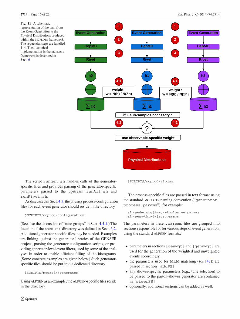
We explain the updates needed for implementation of thenew generator supported by GENSER with the help of thefigure Fig. 11. The figure shows the schematic representa-tion of the path from the Event Generation to the PhysicalDistributions produced within the mcplots framework. Thesequential steps are labelled 1–4.

6.1 Steps 1–3: from the event generation to rivethistograms

Before running the event generation in step 1 of Fig. 11, thegenerator configuration scripts and any other necessary filesshould be set up.

The top-level wrapper script runAll.sh (discussed inSect. 5.1) contains the commands for multiple runs of steps1–3 of the mcplots framework. Generator-specific code andcalls to generator-specific files for steps 1–2 are implementedin the script:

$SCRIPTS/mcprod/rungen.sh .

The third step, executing rivet, is not generator specificand is handled by the script

$SCRIPTS/mcprod/runRivet.sh .

The runRivet.sh relies on rungen.sh and enablesperforming steps 1–3 in one go.

10 http://svnweb.cern.ch/world/wsvn/mcplots/trunk/doc/readme.txt,section on “Adding a new generator”.11 Contact [email protected] for new generator support.

123

http://svnweb.cern.ch/world/wsvn/mcplots/trunk/doc/readme.txt


Fig. 11 A schematicrepresentation of the path fromthe Event Generation to thePhysical Distributions producedwithin the mcplots framework.The sequential steps are labelled1–4. Their technicalimplementation in the mcplotsframework is described inSect. 6

The script rungen.sh handles calls of the generator-specific files and provides parsing of the generator-specificparameters passed to the upstream runAll.sh andrunRivet.sh.

As discussed in Sect. 4.3, the physics process-configurationfiles for each event generator should reside in the directory

$SCRIPTS/mcprod/configuration.

(See also the discussion of “tune groups” in Sect. 4.4.1.) Thelocation of the $SCRIPTS directory was defined in Sect. 3.2.Additional generator-specific files may be needed. Examplesare linking against the generator libraries of the GENSERproject, parsing the generator configuration scripts, or pro-viding generator-level event filters, used by some of the anal-yses in order to enable efficient filling of the histograms.(Some concrete examples are given below.) Such generator-specific files should be put into a dedicated directory

$SCRIPTS/mcprod/(generator).

Using alpgen as an example, the alpgen-specific files residein the directory

$SCRIPTS/mcprod/alpgen.

The process-specific files are passed in text format usingthe standard mcplots naming convention (“generator-process.params”), for example:

alpgenherwigjimmy-winclusive.paramsalpgenpythia6-jets.params.

The parameters in these .params files are grouped intosections responsible for for various steps of event generation,using the standard alpgen formats:

• parameters in sections [genwgt] and [genuwgt] areused for the generation of the weighted and unweightedevents accordingly

• the parameters used for MLM matching (see [47]) arepassed in section [addPS]

• any shower-specific parameters (e.g., tune selection) tobe passed to the parton-shower generator are containedin [steerPS].

• optionally, additional sections can be added as well.

123


Examples of parameter files for W + jets are available onthe mcplots site.

The code responsible for parameter parsing resides in thedirectory:

$SCRIPTS/mcprod/alpgen/utils_alp

which also contains a dictionary of unweighting and MLMmatching efficiencies that enables the generation of a num-ber of final unweighted alpgen + parton-shower events asspecified by the user.

The driver scripts for weighted and unweighted event gen-eration reside in the directory:

$SCRIPTS/mcprod/alpgen/mcrun_alp

This directory also contains generator-level event filters, usedby some of the analyses in order to enable efficient filling ofthe histograms.

The files in the two directories just mentioned, utils_alp/ and mcrun_alp/, are used by the rungen.shscript. The script supports optional additional argumentsbeyond the standard $mode $conf ones (described inSects. 5.1 and 5.2), so that extra generator-specific parame-ters can be included. In the case of alpgen, two extra param-eters are currently given: the parton multiplicity of the matrixelement and inclusive/exclusive matching of the given run.(Tune-specific alpgen parameters are passed at the time ofthe tune setup, see above. The event-generation scripts sup-port the usage of parameters not directly related to the tune.)

The step 2 in Fig. 11 corresponds to ensuring that the out-put of the event generation is provided in the standard eventrecord format: hepmc. For many of the FORTRAN gen-erators, the conversion to the hepmc event record, as wellas utilities for parameter settings and the event generationexecutable, are provided by A Generator Interface Library,agile [48]. The C++ generators are generally able to han-dle these tasks directly. The alpgen event record can bewritten in hepmc format either by invoking agile using theunweighted events as inputs or by using dedicated interfacecode following the alpgen-internal parton shower interfacecode examples and adopting the standard HEPEVT to hepmcconversion utilities. The implementation of the FORTRANgenerators in the agile framework in order to obtain theevents in the hepmc format is not a prerequisite for runningin the mcplots framework. It should however be noted thatusing agile simplifies running of rivet in step 3 in Fig. 11.It is therefore preferred over dedicated interfaces.

agile allows, by setting an input flag, to pass parton levelevents in LHEF format [29] to the supported General PurposeEvent Generators. We thus anticipate that, when showeringevents in LHEF format with FORTRAN event generatorssuch as pythia and herwig, no dedicated code will be nec-essary for the steps 2 and 3 in figure Fig. 11.

6.2 Steps 4.1, 4.2: from single run histograms to physicaldistributions

After the analysis run in step 3 in Fig. 11, the mcplots frame-work merges the single run histograms with the rest of thecompatible analysis runs preceding it (steps 4.1 and 4.2). Insome cases the single run histograms already correspond toPhysical Distributions and the merging is done in order toimprove the statistical precision. In other cases several sin-gle run histograms need to be combined in order to obtainthe Physical Distributions. For the histogram merging it isassumed that the histograms scale linearly with the numberof events.

The merging code is located in:

$SCRIPTS/mcprod/merge.

Once a new source histogram (h0, h1 or h2) in Fig. 11 isobtained, it should be merged to a common destination withthe prior compatible histograms in the database. The run ofthe merging script:

$SCRIPTS/mcprod/merge/merge.sh [source][destination]

handles the merging of the ASCII histogram inputs as well asthe book-keeping of the event multiplicities and the samplecross-section. The merging code runs in two steps as follows:

• first histograms that populate exactly the same regions ofphase-space are merged in order to increase the statisticalprecision of the results. This is denoted as step 4.1 inFig. 11.

• In the second pass of the code, the use-cases where anumber of distinct generation runs are best suited to pop-ulate the phase-space needed for the final histograms arehandled. This is denoted as step 4.2 in Fig. 11. This step isomitted in cases where a single generation run populatesthe whole phase-space.

The source histograms are stored in a directory and namestructure, from which the analysis and generator setup can beinferred. The exact paths are specified in therunRivet.shscript and contain the entries of therivet-histograms.map described in Sect. 4.3 as well as the generator, ver-sion, tune and any generator-specific parameters passed tothe mcplots scripts. The source file path and name thus pro-vide the analysis and generator information to the mergingscript. This information is used in the script to decide whichof the steps to perform and other merging details (detailedbelow).

An example use-case that requires only one pass of themerging code is, the standard one of combining multiple runswith different random-number seeds but otherwise identicalsettings.

123


An example use-case of the run that requires the secondpass of the merging code is filling of the histograms for theproduction of W /Z bosons in association with jets at theLHC, in the context of multi-leg matrix-element matchedsamples. The physics distributions of interest have been mea-sured up to large high-pT jet multiplicities by the LHCexperiments [49–56]. The multi-leg generators such as alp-gen [20], Helac [57], madgraph [58,59], sherpa [26],and Whizard [60] are well suited for the physics case. Foralpgen and madgraph, the efficient population of phase-space needed for prediction of high extra jet multiplicitiesis frequently obtained by producing separate runs with fixednumber of extra partons from the matrix element (Np) thatare passed through the parton shower and hadronization. Inthis way, the high Np sub-samples which are more probableto populate the high extra jet bins in the physics events canbe produced with larger integrated luminosity than the lowNp respectively. A concrete example is the measurement ofW + jets by the ATLAS collaborating [49], where the cross-section decreases by an order of magnitude per extra jet whilethe differential measurement is available for up to ≥ 4 extrajets. Another example requiring the second pass of the merg-ing code is also a combine the physics distributions fromgenerator runs that populate different regions of phase spaceusing generator-level cuts or filters. This is a possible sce-nario for any generator. The merging code and the histogramstructure described in Sect. 3.1 is suited to address such use-cases.

In Fig. 11 the event generation branches in which the his-tograms h0, h1, h2(…) are produced correspond to the sub-samples populating independent phase-space. An exampleare sub-samples with 0, 1, 2(…) extra partons in the case ofalpgen or madgraph in which case the exclusive matchingcriterion must be used for all but the highest multiplicity sub-sample which is matched inclusively. Multiple sub-samplescould also be produced with different phase-space cuts toenhance the number of events in the target corners of thephase-space, such as cuts on the transverse momentum ofthe hard process partons, such that the high-pT events canbe produced with higher integrated luminosity than the low-pT events. The merging code contains a procedure to detectand correctly sum the resulting histograms as illustrated inFig. 11.

The correct merging procedure of the histogram datadepends on the normalization already assumed in the rivetroutines. In practice all the current use-cases could beaddressed by adding two merging modes ALPGEN_XSECTand ALPGEN_FIXED to the merging machinery. TheALPGEN_XSECT mode is used for histograms from rivetruns, when no normalization is performed by rivet. TheALPGEN_FIXED mode is used for histograms that arenormalized according to the cross-section by rivet. The

new histograms from the run with Np partons is mergedwith the existing histograms for the Np sub-sample. Theweights for merging of all the Np samples needed to formthe generator prediction for the observable are than eval-uated such that all the Np sub-samples are normalized tothe same integrated luminosity in ALPGEN_XSECT, or withunit weights for ALPGEN_FIXED mode correspondingly.The choice of the correct merging procedure is implementedin the merging script merge.sh and relies on the his-togram naming conventions. In particular the entries ofrivet-histograms.map, that are constituents of thehistogram path, can serve to assign the correct merging modeaccording to the analysis and generator details. For exam-ple the choice of the merging procedure for currently imple-mented alpgen runs uses the Obs and process fields ofrivet-histograms.map (Sect. 4.3).

The histogram METADATA (e.g. cross-section and thenumber of events) described in Sect. 3.1 is consistentlyupdated with the merged values. In addition the sub-samplespecific fields are added in the format:

samples_X=X_h0:X_h1:X_h2.

Here X denotes a quantity, e.g. cross-section. The X_hdenote the value of the quantity for the individual sub-sample. Hence merging the Np0, Np1, Np2 sub-samplesin ALPGEN_FIXED mode would result in the followingMETADATA for X=crosssection (in [pb]):

crosssection=25554.1samples_crosssection=20831.403148:4285.7315005:436.96532523

It should be noted that the merging in the mcplots needsto proceed on-the-fly, since new samples are produced con-tinuously. This makes the merging more challenging than instandard case, where the final statistics and cross-sections ofall the Np samples is known at the time of analysis and plotproduction. Thus, in the standard case, the Np samples canbe normalized to the same integrated luminosity prior to theplot production, while the mcplots machinery needs to dealwith merging of the already produced plots.

In case the need arises, further merging modes could beadded to the merging structure. For this it is however cru-cial, that the information needed for consistent merging isavailable after the rivet run and correctly transferred to themerging routine. An example piece of such information isthe cross-section in the MLM-matching applications, wherethe final cross-section is only known after the parton shower.Hence, in case the cross-section is not correctly transferredfrom the matrix-element to the parton-shower generator, theautomatic extraction of the information needed for the con-sistent merging would fail.

123


7 LHC@home 2.0 and the Test4Theory project

lhc@home started as an outreach project for CERNs 50thAnniversary in 2004. The project calculated the stability ofproton orbits in the LHC ring, using a software called six-track [61], distributed to volunteers via the Berkeley OpenInfrastructure for Network Computing (BOINC) [37], a pop-ular middleware for volunteer computing. When mcplotswas initially conceived, it was clear that significant sustainedcomputing resources would be needed, and it was natural toconsider if a setup similar to that of sixtrack could be cre-ated to meet those needs. The three main reasons were: 1)the computing resources envisaged for mcplots would havebeen comparable to (or larger than) the total amount of com-puting power then available to the CERN theory group; 2)the developers of lhc@home were keen to explore possibil-ities to expand the volunteer computing framework towardsHEP physics simulations; 3) we saw event simulations asproviding a natural way to involve the public in doing LHCscience, without the complications that would have accom-panied analysis of real data.

A major challenge for the sixtrack project had been theheterogenous nature of the resources provided by volunteers.In particular, it is mandatory to support Windows platforms,which the HEP scientific-computing community is signifi-cantly less familiar with than variants of Linux, UNIX, orMac OSX. In the context of event-generator simulations,we viewed the time-consuming task of porting and main-taining our code over such a large range of platforms asa showstopper. An elegant solution to this problem, whichfactorizes the IT issues almost completely from the scien-tific software development, is virtualization. The develop-ment at CERN of a Scientific-Linux based Virtual-Machinearchitecture (cernvm) along with a generic and scalableinfrastructure for integrating it into cloud-computing envi-ronments (copilot) were the two main innovations thatallowed us to start the test4theory project, which nowprovides the computing backbone for mcplots. This rep-resented the first virtualization-based volunteer computingproject in the world, and, with the new additions, the namewas updated to lhc@home 2.0.

cernvm itself can be installed using any of a num-ber of different so-called virtualization hypervisors (virtual-machine host software), most of which have been designedto add very little overhead to the virtualized simulation. Onethat is open-source and available on all platforms is virtu-albox, which thus is a prerequisite for running simulationsfor test4theory.

The file system of cernvm is designed so that only filesthat are actually accessed are downloaded to the local disk; ahuge virtual library can therefore in principle be made avail-able, without causing a large local footprint or long downloadtimes.

At the time of writing, the lhc@home 2.0 project stilluses BOINC as the main middleware for distributing com-puting jobs to volunteers. What is different with respectto the older sixtrack project is that the BOINC tasks intest4theory are merely wrappers for a VM that is startedup on the remote computer. Each such VM task has a defaultlifetime of 24 h, since volunteers only gain “BOINC credits”each time a BOINC task completes. Inside the wrapper, theVM itself constantly receives jobs, processes them, and sendsoutput back to mcplots. This communication is handled bycopilot.

Alpha testing of the system internally at CERN began inOctober 2010. This first test phase was quite technical, con-centrating on the requirements on the virtual-machine archi-tecture, on the stability and steady supply of jobs, and ondevelopment of the simulation packages themselves. During2011, a small number of external volunteers were graduallyconnected as well, many of whom participated actively intesting and debugging this first edition of the system. By theend of the alpha test stage, in July 2011, the system oper-ated smoothly and continuously with about 100 machinesconnected from around the globe.

During beta testing, in the latter half of 2011, the main lineof attack was the scalability of the system. In a first beta trial inAugust 2011, the system was opened up to the broader publicin combination with a press release from CERN. This resultedin such a massive amount of new subscriptions that the systemthen in place could not handle it, resulting in crashes. A pro-cedure was then introduced by which volunteers wishing toparticipate could sign up for participation codes which wereissued incrementally. This gradually brought the number ofconnected participants up to around 2,500, while we wereable to monitor and improve the scalability significantly. Dur-ing its second phase, the participation-code restriction wasremoved, and the number of successfully connected hostsincreased to about 6,500 machines by the end of the beta trial(with a noticeable spike around the CERN Press Release onDec 13, 2011 concerning the possible hints of a Higgs boson;another significant spike was seen on July 4th 2012, whenthe discovery was confirmed).

The system is now fully operational, with several thousandvolunteers donating CPU cycles on a daily basis, and indi-vidual volunteers already having generated billions of eventseach, cf. the Test4Theory Leaderboard reproduced in Fig. 12.At the time of writing, in June 2013, the number of volunteerswho have completed at least one work package is 8,000, witha combined total of roughly 13,500 machines. The numberof instantaneously connected machines fluctuates between600–800.

These contributions have made a crucial difference inbeing able to generate the massive amounts of statisticsrequired for the innumerable combinations of generators,tunes, and experimental analyses provided on mcplots.

123


Fig. 12 test4theoryLeaderboard (top contributors innumber of events generated), asof May 2013. The up-to-dateonline version can be consultedat [40].

8 Conclusions

In this paper, we have provided an elementary user guidefor the mcplots site, and summarized its technical imple-mentation. We intend the site to be broadly useful to theparticle physics community, as a resource for MC valida-tion and tuning, and as an explicit browsable repository ofrivet analyses. It also provides a possibility for the publicto engage in the scientific process, via the lhc@home 2.0project test4theory.

In the near future, we plan to extend the site by addingmore possibilities for users to create their own plots andcontrol how they look. We will also aim to provide event-generator authors with a pre-release validation service, inwhich a would-be new version of a generator or tune param-eter card can be uploaded securely and a private version of thesite made available on which the corresponding results canbe compared with the standard set of generators and tunes.

Plans for future developments of test4theory includeminimizing the size of the downloadable cernvm imagefor test4theory (μcernvm), a new delivery method fortest4theory that would allow one to download, install,and run test4theory directly from a web browser(test4theoryDirect), and the development of a new inter-active citizen-science application based on the test4theoryframework.

Note to users of mcplots: we are of course very grate-ful if a reference to this work is included when using con-tent from mcplots, but even more importantly, we ask ourusers to please acknowledge the original sources for the data,analyses, physics models, and computer codes that are dis-played on mcplots. We have tried to make this as easyas possible, by including links to the original experimen-

tal papers together with each plot. Other references that maybe appropriate, depending on the context, include hepdata[13], rivet [14], MC generator manuals [20–26], and rele-vant physics and/or tuning papers.

As an example of good practice, and to ensure maxi-mal clarity and reproducibility, all plots on mcplots includeexplicit generator names and version numbers for all curvesappearing on the plot, together with the relevant experimentalreference. When combining an ME generator X with a (dif-ferent) shower generator Y, both names and version numbersare shown explicitly. This is not only to give proper credit tothe authors, but since the physics interpretation of the calcu-lation depends on how it was performed.

Acknowledgments We are indebted to many members of the MonteCarlo community for their feedback and help with validations of thegenerators and analyses included on mcplots. Many short-term stu-dents, visitors, and fellows have contributed with rivet analyses andother content to the site, in particular D. Konstantinov (the mcplotsplotting tool), A. Pytel (server infrastructure and the MC validationview), S. Sen (forward LHC analyses in rivet and on mcplots, andimplementation of the epos and phojet generators), and J. Winter(the t t̄ MC analyses). We thank J. Katzy, for carefully reading thismanuscript and giving feedback on the mcplots site, M. Mangano,for his strong support of this project from its inception to completionand for help with the alpgen implementation, and T. Pierog, for helpwith the epos implementation. We express our profound admirationof the teams responsible for the development of rivet, cernvm, andlhc@home 2.0, without which the test4theory project would havebeen impossible. Thanks also to the many volunteers who have pro-vided computing resources, especially to those who have taken activepart in the alpha and beta testing phases of test4theory. We alsothank the CERN PH-SFT group, in particular the Generator Services(GENSER) team, and the CERN IT Division. This work was supportedin part by the LHC Physics Center at CERN (LPCC), by the MarieCurie research training network “MCnet” (contract number MRTN-CT-2006-035606), and by the National Science Foundation under GrantNo. NSF PHY11-25915.

123


Open Access This article is distributed under the terms of the CreativeCommons Attribution License which permits any use, distribution, andreproduction in any medium, provided the original author(s) and thesource are credited.Funded by SCOAP3 / License Version CC BY 4.0.

References

1. A. Buckley, J. Butterworth, S. Gieseke, D. Grellscheid, S. Höcheet al., MCnet Collaboration, General-purpose event generators forLHC physics. Phys. Rep. 504, 145–233 (2011). [arXiv:1101.2599]

2. P. Skands, Introduction to QCD, 1207.2389. Lectures given at TASI2012

3. M.H. Seymour, M. Marx, Monte Carlo event generators,1304.6677. Lectures given at 69th Scottish UniversitiesGÇÖ Sum-mer School in Physics

4. A. Buckley, H. Höth, H. Lacker, H. Schulz, J.E. von Seggern, Sys-tematic event generator tuning for the LHC. Eur. Phys. J. C65,331–357 (2010). [arXiv:0907.2973][hep-h].

5. P.Z. Skands, Tuning Monte Carlo generators: the Perugia tunes.Phys. Rev. D82, 074018 (2010). [arXiv:hep-th/1005345]

6. R. Corke, T. Sjöstrand, Interleaved parton showers and tuningprospects. JHEP 1103, 032 (2011). [arXiv:1011.1759]

7. S. Gieseke, C.A. Rohr, A. Siodmok, Tuning of the multiple partoninteraction model in Herwig++ using early LHC data. In: Proceed-ings of MPI@LHC 2011, DESY-PROC-2012-03

8. H. Schulz, P. Skands, Energy scaling of minimum-bias tunes. Eur.Phys. J. C71, 1644 (2011). [arXiv:1103.3649]

9. ATLAS Collaboration, Summary of ATLAS Pythia 8 tunes, ATL-PHYS-PUB-2012-003, ATL-COM-PHYS-2012-738

10. J. Alcaraz Maestre et al., The SM and NLO multileg and SM MCworking groups: summary report [arXiv:1203.6803]

11. G.P. Salam, Elements of QCD for hadron colliders, 1011.5131.Lectures given at ESHEP 2009

12. J. Butterworth, S. Butterworth, JetWeb: a WWW interface anddatabase for Monte Carlo tuning and validation. Comput. Phys.Commun. 153, 164–178 (2003). [arXiv:hep-ph/0210404]

13. A. Buckley, M. Whalley, HepData reloaded: reinventing the HEPdata archive [1006.0517]. http://durpdg.dur.ac.uk/

14. A. Buckley, J. Butterworth, L. Lönnblad, D. Grellscheid, H. Höthet al., Rivet user manual. Comput. Phys. Commun. 184, 2803–2819(2013). [arXiv:1003.0694]

15. M. Dobbs, J.B. Hansen, The HepMC C++ Monte Carlo event recordfor High Energy Physics. Comput. Phys. Commun. 134, 41–46(2001)

16. M. Cacciari, G.P. Salam, Dispelling the N 3 myth for the kt jet-finder. Phys. Lett. B641, 57–61 (2006) [arXiv:hep-ph/0512210].http://fastjet.fr

17. M. Cacciari, G.P. Salam, G. Soyez, FastJet user manual. Eur. Phys.J. C72, 1896 (2012). [arXiv:1111.6097]

18. M. Whalley, D. Bourilkov, R. Group, The Les Houches accordPDFs (LHAPDF) and LHAGLUE [arXiv:hep-ph/0508110]

19. D. Bourilkov, R.C. Group, M.R. Whalley, LHAPDF: PDF use fromthe Tevatron to the LHC [arXiv:hep-ph/0605240]

20. M.L. Mangano, M. Moretti, F. Piccinini, R. Pittau, A.D. Polosa,ALPGEN, a generator for hard multiparton processes in hadroniccollisions. JHEP 0307, 001 (2003). [arXiv:hep-ph/0206293]

21. K. Werner, I. Karpenko, T. Pierog, M. Bleicher, K. Mikhailov,Event-by-event simulation of the three-dimensional hydrodynamicevolution from flux tube initial conditions in ultrarelativistic heavyion collisions. Phys. Rev. C82, 044904 (2010). [arXiv:1004.0805]

22. M. Bähr, S. Gieseke, M. Gigg, D. Grellscheid, K. Hamilton et al.,Herwig++ physics and manual. Eur. Phys. J. C58, 639–707 (2008).[arXiv:0803.0883]

23. F.W. Bopp, R. Engel, J. Ranft, Rapidity gaps and the PHOJETMonte Carlo [arXiv:hep-ph/9803437]

24. T. Sjöstrand, S. Mrenna, P.Z. Skands, PYTHIA 6.4 physics andmanual. JHEP 0605, 026 (2006). [arXiv:hep-ph/0603175]

25. T. Sjöstrand, S. Mrenna, P. Skands, A brief introduction to PYTHIA8.1. Comput. Phys. Commun. 178, 852–867 (2008). [arXiv:0710.3820]

26. T. Gleisberg, S. Höche, F. Krauss, M. Schonherr, S. Schumann etal., Event generation with SHERPA 1.1. JHEP 0902, 007 (2009).[arXiv:0811.4622]

27. W. Giele, D. Kosower, P. Skands, Higher-order corrections to time-like jets. Phys. Rev. D84, 054003 (2011). [arXiv:1102.2126]

28. E. Boos, M. Dobbs, W. Giele, I. Hinchliffe, J. Huston, et al.,Generic user process interface for event generators [arXiv:hep-ph/0109068]

29. J. Alwall, A. Ballestrero, P. Bartalini, S. Belov, E. Boos et al., Astandard format for Les Houches event files. Comput. Phys. Com-mun. 176, 300–304 (2007). [arXiv:hep-ph/0609017]

30. LHC@home 2.0. http://lhcathome2.cern.ch/31. B. Segal, P. Buncic, D.G. Quintas, C. Aguado Sanchez, J. Blomer,

et al., LHC cloud computing with CernVM, PoS ACAT2010, 004(2010)

32. C. Aguado Sanchez, J. Blomer, P. Buncic, G. Chen, J. Ellis et al.,Volunteer clouds and citizen cyberscience for LHC physics. J. Phys.Conf. Ser. 331, 062022 (2011)

33. D. Lombraña Gonzalez, F. Grey, J. Blomer, P. Buncic, A. Haru-tyunyan, et al., Virtual machines and volunteer computing: expe-rience from LHC@Home: Test4Theory project, PoS ISGC2012,036 (2012)

34. P. Buncic, C. Aguado Sanchez, J. Blomer, L. Franco, A. Harutyu-nian, et al., CernVM: a virtual software appliance for LHC applica-tions. J. Phys. Conf. Ser. 219, 042003 (2010). http://cernvm.cern.ch

35. A. Harutyunyan, J. Blomer, P. Buncic, I. Charalampidis, F. Grey etal., CernVM Co-Pilot: an extensible framework for building scal-able computing infrastructures on the cloud. J. Phys. Conf. Ser.396, 032054 (2012)

36. A. Harutyunyan, C. Aguado Sanchez, J. Blomer, P. Buncic,CernVM Co-Pilot: a framework for orchestrating virtual machinesrunning applications of LHC experiments on the cloud. J. Phys.Conf. Ser. 331, 062013 (2011)

37. The BOINC Project. http://boinc.berkeley.edu38. N. Hoimyr, J. Blomer, P. Buncic, M. Giovannozzi, A. Gonzalez et

al., BOINC service for volunteer cloud computing. J. Phys. Conf.Ser. 396, 032057 (2012)

39. The Generator Services Project. http://sftweb.cern.ch/generators/40. The Test4Theory Project. http://lhcathome2.cern.ch/

about-test4theory41. ALICE Collaboration, K. Aamodt et al., Charged-particle multi-

plicity measurement in proton-proton collisions at√

s = 7 TeVwith ALICE at LHC. Eur. Phys. J. C68, 345–354 (2010) [arXiv:1004.3514]

42. ATLAS Collaboration, G. Aad et al., Charged-particle multiplic-ities in pp interactions measured with the ATLAS detector at theLHC. New J. Phys. 13, 053033 (2011) [arXiv:1012.5104]

43. ATLAS Collaboration, G. Aad et al., Measurement of underly-ing event characteristics using charged particles in pp collisions at√

s = 900GeV and 7 TeV with the ATLAS detector. Phys. Rev.D83, 112001 (2011) [arXiv:1012.0791]

44. B. Cooper, J. Katzy, M. Mangano, A. Messina, L. Mijovic et al.,Importance of a consistent choice of alpha(s) in the matching ofAlpGen and Pythia. Eur. Phys. J. C72, 2078 (2012). [arXiv:1109.5295]

45. OPAL Collaboration, K. Ackerstaff et al., Measurements of flavordependent fragmentation functions in Z0 to q anti-q events. Eur.Phys. J. C7, 369–381 (1999) [arXiv:hep-ex/9807004]

123

http://arxiv.org/abs/arXiv:1101.2599


http://arxiv.org/abs/arXiv:hep-th/1005345




http://arxiv.org/abs/arXiv:hep-ph/0210404

http://durpdg.dur.ac.uk/



http://fastjet.fr
















http://lhcathome2.cern.ch/

http://cernvm.cern.ch

http://cernvm.cern.ch

http://boinc.berkeley.edu

http://sftweb.cern.ch/generators/

http://lhcathome2.cern.ch/about-test4theory

http://lhcathome2.cern.ch/about-test4theory







http://arxiv.org/abs/arXiv:hep-ex/9807004


46. CDF Collaboration, D. Acosta et al., Study of jet shapes in inclusivejet production in p p̄ collisions at

√s = 1.96 TeV. Phys. Rev. D71,

112002 (2005) [arXiv:hep-ex/0505013]47. M.L. Mangano, M. Moretti, F. Piccinini, M. Treccani, Matching

matrix elements and shower evolution for top-quark productionin hadronic collisions. JHEP 0701, 013 (2007). [arXiv:hep-ph/0611129]

48. The AGILe Project. http://agile.hepforge.org49. ATLAS Collaboration, G. Aad et al., Measurement of the produc-

tion cross section for W − bosons in association with jets in ppcollisions at

√s = 7 TeV with the ATLAS detector. Phys. Lett.

B698, 325–345 (2011) [arXiv:1012.5382]50. CMS Collaboration, S. Chatrchyan et al., Study of the dijet mass

spectrum in pp → W+ jets events at√

s = 7 TeV. Phys. Rev.Lett. 109, 251801 (2012) [arXiv:1208.3477]

51. C.M.S. Collaboration, S. Chatrchyan et al., Event shapes andazimuthal correlations in Z + jets events in pp collisions at

√s = 7

TeV. Phys. Lett. B722, 238–261 (2013). [arXiv:1301.1646]52. ATLAS Collaboration, G. Aad et al., Measurement of kT splitting

scales in W − → �ν events at√

(s) = 7 TeV with the ATLASdetector. Eur. Phys. J. C73, 2432 (2013) [arXiv:1302.1415]

53. ATLAS Collaboration, G. Aad et al., Measurement of the cross-section for W boson production in association with b-jets in ppcollisions at

√s = 7 TeV with the ATLAS detector. JHEP 1306,

084 (2013) [arXiv:1302.2929]54. CMS Collaboration, S. Chatrchyan et al., Studies of jet mass in

dijet and W/Z + jet events. JHEP 1305, 090 (2013) [arXiv:1303.4811]

55. ATLAS Collaboration, G. Aad et al., Measurement of the pro-duction cross section of jets in association with a Z boson in ppcollisions at

√s = 7 TeV with the ATLAS detector. JHEP 1307,

032 (2013) [arXiv:1304.7098]56. CMS Collaboration, S. Chatrchyan et al., CMS Collaboration Mea-

surement of the hadronic activity in events with a Z and two jetsand extraction of the cross section for the electroweak productionof a Z with two jets in pp collisions at

√s = 7 TeV. JHEP 1310,

101 (2013) [arXiv:1305.7389]57. A. Cafarella, C.G. Papadopoulos, M. Worek, Helac-Phegas: a gen-

erator for all parton level processes. Comput. Phys. Commun. 180,1941–1955 (2009). [arXiv:0710.2427]

58. J. Alwall, P. Demin, S. de Visscher, R. Frederix, M. Herquet et al.,MadGraph/MadEvent v4: the new web generation. JHEP 0709,028 (2007). [arXiv:0706.2334]

59. J. Alwall, M. Herquet, F. Maltoni, O. Mattelaer, T. Stelzer, Mad-Graph 5: going beyond. JHEP 1106, 128 (2011). [arXiv:1106.0522]

60. W. Kilian, T. Ohl, J. Reuter, WHIZARD: simulating multi-particleprocesses at LHC and ILC. Eur. Phys. J. C71, 1742 (2011). [arXiv:0708.4233]

61. G. Robert-Demolaize, R. Assmann, S. Redaelli, F. Schmidt, A newversion of SixTrack with collimation and aperture interface. Conf.Proc. C0505161, 4084 (2005)

123

http://arxiv.org/abs/arXiv:hep-ex/0505013



http://agile.hepforge.org















Documents

MCPLOTS: a particle physics resource based on volunteer computing