ME 160 Introduction to Finite Element Method Chapter 5 ... Conduc.pdf · Finite Element Analysis in Heat Conduction Analysis of Solid Structures ... and h is the heat transfer coefficient

Chapter 5

Finite Element Analysis in Heat Conduction Analysis of Solid Structures

Instructor

Tai-Ran Hsu, Professor

San Jose State University Department of Mechanical Engineering

ME 160 Introduction to Finite Element Method

Principal references: 1) “The Finite Element Method in Thermomechanics,” by T.R.Hsu, Allen & Unwin, Boston, 1986. ISBN

0-04-620013-4 (SJSU Library: TA418.58 H78 1986 at 8th Floor with one reserved copy at 1st Floor), Chapter 2.

2) “Chapter 2 Finite Element Equations for Heat Transfer,” by G.P. Nikishkov, Springer,http://springer.com/978-1-84882-971-8

3) “Applied Finite Element Analysis” L. J. Segerlind, John Wiley & Sons, 1976

Introduction to Fundamentals of Heat Conduction in Solids

Part 1

Fourier law of heat conduction

A natural phenomenon is that heat flows in a solid is possible only with temperature gradients with heat from the

locations at higher temperature to the locations with lower temperature. Consequently, heat will flow from the left side

to the right side of the slab if we maintain the situation of Ta > Tb with Ta and Tb being the temperature at left and right

faces of the slab respectively as illustrated below:

Amount of

heat flow, QQ

d

Area, A

d

tTTAQ ba )(

Ta

Tb

d

tTTAkQ ba )(

=

where K = Thermal conductivity of material with units of: Btu/in-s-oF in the traditional system, or w/m-oC in the SI system.

d

TTk

At

Qq ba )(

Fourier law of heat conduction-cont’d

Instead of total heat flow, a more commonly used terminology in engineering analysis is “heat flux” defined as “heat flow in solid per unit area and time.” Mathematically, it is expressed as:

for heat flow in a solid slab – a vector quantity

For continuous variation of temperature between the two faces and let the coordinate along the length of the slab be x-axis, we will have the above expression in the form of:

T(x)

X

x

0

x + ΔxΔx

Ta Tb

T(x) T(x + Δx)

Heat flow: Ta > Tb

T(x)

d

x

xTxxTk

x

xxTxTkq

)()()()(

with “contiguous” variation of temperature, the following expression prevails:

dx

xdTkxqq

)()( (5.1)

Equation (5.1) is the mathematical expression of the “Fourier Law of Heat Conduction”

Fourier law of heat conduction in 3-D space

x

y

z q(r,t)

qx

qy

qz

Position vector:

r: (x,y,z)

tTktq ,, rr (5.2)

x

tzyxTkq xx

),,,(

y

tzyxTkq yy

),,,(

z

tzyxTkq zz

),,,(

with components: (5.3a)

(5.3b)

(5.3c)

T(x,y,z,t)

qqqtzyxqzyx

222),,,(

The resultant total heat flux in the solid in Equation (5.2) is the vector sum of the components in Equation (5.3) To be:

where kx, ky and kz are the thermal conductivity of the material along the respective x-, y- and z-directions. For isotropic materials, we will have k = kx=ky=kz

Heat Conduction Equation in Solids

q1

q2

q3

q4

Q(r,t)

T(r,t)

x

y

z

0

Given a solid situated in a space defined by a coordinate system (r,t) or (x,y,z,t) Heat fluxes in and out of the solid by q1, q2, q3,…….., and heat generated in the solid by the amount Q(x,y,z,t) per unit volume and unit time. There will be induced temperature distribution (or temperature field) in the solid by T(r,t) or T(x,y,z,t) in the solid.

The heat conduction equation was derived using the Fourier law of heat conduction and on the basis of law of conservation of energies t

TcQ

z

q

y

q

x

q zyx

Now, if we substituting the heat fluxes shown in Equations (5.2) and (5.3) into the above expression to yield:

t

tzyxTctzyxQ

z

tzyxTk

zy

tzyxTk

yx

tzyxTk

x

,,,,,,

,,,,,,,,, (5.5)

Equation (5.4) is the heat conduction equation for solids, in which ρ is the mass density and c is the specific heat of the material

For steady-state heat conduction in the solid:

0,,,

,,,,,,,,,

tzyxQ

z

tzyxTk

zy

tzyxTk

yx

tzyxTk

x(5.6)

The term Q(x,y,z,t) in both Equations (5.4) and (5.5) is the heat GENERATED by the solid, such as by Ohm’s heating or nuclear fission

(5.4)

t

tzyxTctzyxQ

z

tzyxTk

zy

tzyxTk

yx

tzyxTk

x

,,,,,,

,,,,,,,,,

Heat Conduction Equation in Solids with specific conditions

The Heat conduction equation:

(5.5)

The boundary conditions:

(1) Specified temperature on the boundary surface S1: Ts = T1(x,y,z,t) on S1

(2) Specified heat flow on the boundary surface S2:

qxnx+qyny+qznz=-qs on S2 (nx=cosine to outward normal line in x-direction)

(3) Specified convective boundary condition on the boundary surface S3:

qxnx+qyny+qznz=h(Ts-Tf) on S2

The initial conditions: T(x,y,z,0) = To(x,y,z)

(5.7a)

(5.7b)

(5.7c)

(5.7d)

In the above boundary conditions, qs in Equation (5.7b) is the heat flux across the boundary from external sources, and h is the heat transfer coefficient of the surrounding fluid at bulk fluid temperature Tf for convective boundary condition over surface S3.

Finite Element Formulations

Part 2

Finite element formulation of heat conduction in solid structures

The primary unknown quantity in finite element analysis of heat conduction in solid structures is the TEMPERATURE in the elements and NODES.

As usual, the very first step in FE analysis is to discretize the continuum structure into discretized FE model such as illustrated below:

q1

q2

q3

q4

Q(r,t)

T(r,t)

x

z

0

q1

q2

q3

q4

Q(r,t) T(r,t)

x

z

0

Continuum solid Discretized FE model

T(r,t)

Element temperature ●

● ●

●

Nodal Temperature:

Tk

Tj Ti

Tm

x

y

z

0

y y Typical element

Finite element formulation of heat conduction in solid structures – cont’d

The Interpolation Function, [N(x,y,z]:

The same definition of interpolation function for stress analysis is used for the heat conduction analysis, i.e.:

Element Temperature, T =

Interpolation Function [N(x,y,z)]

Nodal

Temperature {T}

where the interpolation function: [N(x,y,z)] = { Ni Nj Nk Nm} The nodal temperature: {T} = {Ti Tj Tk Tm}T

(5.8)

(5.9)

(5.10)

The temperature gradients in the element may be obtained in terms of nodal temperature by differentiate the relationship in Equation (5.8) as:

TBT

z

N

z

N

z

N

z

N

y

N

y

N

y

N

y

Nx

N

x

N

x

N

x

N

z

zyxT

y

zyxTx

zyxT

mkji

mkji

mkji

,,

,,

,,

(5.11)

where the matrix [B] has the form:

z

N

z

N

z

N

z

N

y

N

y

N

y

N

y

Nx

N

x

N

x

N

x

N

B

mkji

mkji

mkji

(5.12)


The functional for deriving element equations:

Because the conduction of heat in solids can be completely described by simple differential equations such as

t

tzyxTctzyxQ

z

tzyxTk

zy

tzyxTk

yx

tzyxTk

x

,,,,,,

,,,,,,,,, (5.5)

for transient state, and

0,,,

,,,,,,,,,

tzyxQ

z

tzyxTk

zy

tzyxTk

yx

tzyxTk

x(5.6)

for steady-state, and the boundary and initial conditions expressed in Equations (5.7), Galerkin method such as described in Chapter 3 will be used to derive the element equation. We will first review the Galerkin method in the next slide.

Step 4 – Chapter 3 Galerkin method

Real Situation on solids Approximate situation: Discretized Situation with elements

In contrast to the Rayleigh-Ritz method, this method is used to derive the element equations for the cases in which specific differential equations with appropriate mathematical expressions for the boundary conditions available for the analytical problems, such as heat conduction and fluid dynamic analyses

Differential Equation: D(Φ) for the volume V (5.4) Differential Equation: D(N(r)Φ) for the element volume V

Boundary condition: B(Φ) for the real situation on boundary S (5.5)

Boundary condition: B(N(r)Φ) for the real situation on element boundary

Mathematical model: 0 dsBWdvDWsv

Mathematical model: dsNBWdvNDW iis

jiiv

j )( rr = R

Element Φ(r)

Nodal {Φ}

Φ(r) = N(r)Φ

where functionsweightingarbitralyareWandW sidualtheisRandfunctionsweightingddiscretizeareWandW jj Re,

Galerkin method lets )(rNWandW jj

zyx ,,:r

and let R to be minimum, or R→ 0 for good discretization, resulting in:

[Ke] {q} = {Q} The same element equation:

[N(r)] in Equation (5.9)


Derivation of Element Equation using Galerkin Method

Using the Galerkin method, we can rewrite the basic heat conduction equation in the following form:

0

dvN

t

TcQ

z

q

y

q

x

qi

v

zyx

Equation (5.4)

Equation (5.9)

By incorporate the boundary conditions in Equations (5.7) in the above equation will result in the element equation with the balanced of heat flus across the boundary and the induced temperature in the element in the following equation:

dsNTThdsNqdsNnqdvNQdvq

z

N

y

N

x

NdvN

t

tzyxTc

sif

sisi

T

si

vv

iiii

v

321

),,,

with zyx

T

zyx

Tnnnnnorrmaloutwardtoinedirectiontheandqqqqboundariesacrossfluxheat cos

(5.13)


Derivation of Element Equation using Galerkin Method – cont’d

The heat balance in Equation (5.13) may be lumped to the following element equation:

hqThc RRRTKKTC (5.14)

where in the coefficient matrices:

dsNNhKmatrixconvectiveThe

dvBBkKmatrixtycondictiviThe

dvNNcCmatrixcapcitnceheatThe

S

T

h

T

vc

T

v

3

:

:

:

and the nodal thermal force matrices:

dsNhTRSboundarythecrossfluxheatconvectiveThe

dsNqRSboundarytheacrossfluxheatThe

dvNQRmatrixgenerationheatThe

dsNnqRSboundarytheacrossfluxheatThe

T

Sfh

T

Ssq

T

vQ

T

S

T

T

3

2

1

:

:

:

:

3

2

1

(5.15a)

(5.15b)

(5.15c)

(5.16a)

(5.16b)

(5.16c)

(5.16d)

Heat Conduction in Planar Structures Using Finite Element Method

Part 3

Finite element formulation of heat conduction in solid structures in planes

qs

Heat conduction in a tapered plate:

● ● ●

● ● ● ●

●

●

● ● ● ●

● ● ● ● ●

●

●

●

ο

ο

ο

ο X 1 2 3 4 5 6 7

8 9 10 11 12 13 14

15 16 17

18 19 20 21

22 23 24 25

1 2 3 4 5 6

7 8 9 10 11 12

13 14

15 16

17 18

qs

FE Mesh

L

H

L1

r Ts

h(Ts-Tf)

T(x,y,t) x

y

h(Ts-Tf)

Ts

Ts

Ts

●

●

● T(x,y)

T1(x1,y1)

T2(x2,y2)

T3(x3,y3)

x

y

0

FE formulation in a triangular plate element: Element temperature: T(x,y) Nodal temperature: T1(x1,y1); T2(x2,y2); T3(x3,y3)

Finite element formulation of heat conduction in solid structures in planes

FE formulation in a triangular plate element-The interpolation function:

T

RyxyxyxT

3

2

1

321 1,

We assume the element temperature T(x,y) is represented by a simple linear polynomial function that:

(5.17)

where α1, α2, and α3 are constants

yxRT

1with (5.18)

Because the coordinates (x1,y1), (x2,y2) and (x3,y3) of the nodes in a FE mode are fixed. We may substitute these coordinates into Equation (5.17) and obtain the following expressions for the corresponding quantities at the three nodes:

1131211 NodeforyxT

2232212 NodeforyxT

3333213 NodeforyxT

or in a matrix form for nodal temperatures: AT (5.19)

and the unknown coefficients ThTA 1

(5.20)

The matrix [A] in Equations (5.19) and (5.20) contains the coordinates of the three nodes as:

33

22

11

1

1

1

yx

yx

yx

A

Finite element formulation of heat conduction in solid structures in planes – cont’d

FE formulation in a triangular plate element – the interpolation function - cont’d:

The inversion of matrix [A]-1 = [h] can be performed to give:

123123

211332

1221311323321

xxxxxx

yyyyyy

yxyxyxyxyxyx

Ah

where A Is the determinant of the element of matrix [A] Ayxyxyxyxyxyx 2311323321221

with A= the area of triangle made by (T1T2T3)

(5.21)

By substituting (5.21) into (5.20) and then (5.19), the element quantity represented by T(x,y) can be made to equal the corresponding nodal quantities {T}: T1, T2, T3 to be:

ThRyxTT

,



We will thus have the interpolation function: N(x,y) = {R}T[h] with {R}T = {1 x y} in Equation (5.18) and [h} given in Equation (5.21)

We thus have the relationship between the element quantity to the nodal quantifies by the following expression: T(x,y) = {N(x,y)} {T} or express the above equation in the form according to Equation (5.8) as:

333

222

111

321

,

,

,

,,,,

yxT

yxT

yxT

yxNyxNyxNyxT

(5.22)

(5.23)

with ycxbaA

NycxbaA

NycxbaA

N 3333222211112

1,

2

1,

2

1

3123122113322 yxyxyxyxyxyxA

(5.24)

and

12321312213 xxcyybyxyxa

)()(22 321311323321221 TTTtriangleofmadeAelementtheofareatheyxyxyxyxyxyxA



333

222

111

321

,

,

,

,,,,

yxT

yxT

yxT

yxNyxNyxNyxT

with ycxbaA

NycxbaA

NycxbaA

N 3333222211112

1,

2

1,

2

1



(5.23)

(5.25a)

(5.25b)

(5.25c)


FE formulation in a triangular plate element – The element coefficient matrix:

The conductivity matrix [Kc]:

By following Equation (5.15b), we have the conductivity matrix for a triangular plate element to be:

A

T

c dxdyBBkK (5.26)

The temperature gradient matrix [B] can be obtained by the following formulation:

321

321

321

3121

2

1

ccc

bbb

Ay

N

y

N

y

Nx

N

x

N

x

N

B (5.27)

We may obtain the conductivity matrix by substituting Equation (5.27) into Equation (5.26), leading to:

2

3

2

332323131

3232

2

2

2

22121

31312121

2

1

2

1

24cbccbbccbb

ccbbcbccbb

ccbbccbbcb

A

kKc (5.28)


FE formulation in a triangular plate element – The element equations:

As in the case of stress analysis in chapter 4, the element equations for heat conduction solids of plenary geometry may be shown to take the form:

qTKe (5.29)

where [Ke} = coefficient matrix in Equation (4.28), {T} = nodal temperature, and {q} = thermal forces at the nodes

The thermal forces at nodes are: {q} = {fQ} + {fq} = (fh}

in which {fQ} = heat generation in the solid with

1

1

1

3

QvdvNQQdvNf

T

vv

T

Q

{fq} = heat flux across boundary with

22 S

m

j

iT

Sq ds

N

N

N

qqdsNf

{fh} = convective heat flux across boundary with dshTNfS

f

T

h 3

(5.30)

(5.31a)

(5.31b)

(5.31c)

0

1

1

2

tqL jifor side i-j

1

1

0

2

tqL mj for side j-m

1

0

1

2

tqL im for side m-i

where t = thickness of the plane

Example 5.1

HOT

Cool

HOT

Cold

Use finite element method to determine the temperature variation across the thickness of longitudinal fins of a tubular heat exchanger as shown in the figure on the left. The heat exchanger is designed to heat up the cold fluid outside the tube by the hot fluid circulating inside the tube. The cross-section of a single fin is illustrated in the figure shown in lower-left of this slide.

The fin is made of aluminum with the properties: Mass density ρ = 2.7 g/cm3 , Specific heat c = 0.942 J/g-oC, and thermal conductivity k = 2.36 W/cm-oC

4 cm

2 cm

qs Convective BC

h, Tf

Convective BC h, Tf

The discretized FE model of the fin cross-section is shown below:

• •

• •

1

2

1(0,0) 2(2,0)

3(2,4) 4(0,4)

X

y Convective BC

h, Tf

Convective BC h, Tf

Heat flux qs

qs = 10 kW/m2

h = 20 W/m2-oC

Tf = 40oC

Boundary conditions:

Tube with one longitudinal fin

Example 5.1-cont’d

Interpolations functions for Elements:

We will use Equations (5.25a,b,c) to determine the constant coefficients ai, bi and ci (I = 1,2,3) for each element. These coefficients will then be used to express the interpolation function of both Element 1 and 2, as in Equation (5.23). We realize the following nodal coordinates in the FE model of the fin: For element 1 (Node 1, 2 and 3): x1 = 0, y1 = 0; x2 = 2, y2 = 0; x3 = 2, y3 = 4 The area A of the cross-section area of Element 1 is computed by using the expression:

84002024202002 311323321221 yxyxyxyxyxyxA

This leads to A = 4 cm2

We will further compute the constant coefficients by the following expressions:

02244040222 23132123321 xxcyybyxyxa

22040404004 31213231132 xxcyybyxyxa

20200000200 12321312213 xxcyybyxyxa


Interpolations functions for Elements:

For Element 2 (Node 1, 3 and 4): x1 = 0, y1 = 0; x3 = 3, y3 = 4; x4 = 0, y4 = 4 The area A of the cross-section area of Element 2 is the same as of Element 1 = 4 cm2. the constant coefficients are determined the same way as for those in Element 1.

330044124043 23132123321 xxcyybyxyxa

00040404000 31213231132 xxcyybyxyxa

30344000340 12321312213 xxcyybyxyxa

We will thus have the interpolation functions for both element 1 and 2 by substituting the constant coefficients into Equation (5.23):

For Element 1:

yyxN

yxyxN

xyxN

25.020042

1

25.024042

1

5.05.004442

1

3

2

1

Leads to:

3

2

1

1 25.05.0(5.05.0

T

T

T

yyxxTe (a)

For Element 2:

yxyxN

xyxN

yyxN

375.05.034042

1

5.004042

1

375.05.1301242

1

4

3

1

Leads to:

4

3

1

2 375.05.05.0375.05.1

T

T

T

yxxyTe (b)


Element coefficient matrices [Ke]:

We will use Equation (5.28) to derive these matrices.

2

3

2

332323131

3232

2

2

2

22121

31312121

2

1

2

1

24cbccbbccbb

ccbbcbccbb

ccbbccbbcb

A

kKc (5.28)

For Element 1:

15.015.00

15.02.16.0

06.06.0

)2(0)2)(2()0)(4()2)(0()0)(4(

)2)(2()0)(4()2(4)2)(0()4)(4(

)2)(0()0)(4()2)(0()4)(4(04

44

36.2

22

22

22

2

1

eK (C)

Node: 1 2 3

1 2 3

For Element 2:

7375.06.01475.0

6.06.00

1475.001475.0

)2()4()2)(0()4)(4()2)(2()4)(0(

)2)(0()4(404)0)(2()4)(0(

)2)(2()4)(0()0)(2()4)(0(20

44

36.2

22

22

22

2

2

eK

Node: 1 3 4

1 3 4

(d)

Example 5.1-cont’d Assembly of element coefficient matrices for Overall coefficient (conductance) matrix

Elements in Node 1 2 3 4 1 2 3 4

1

2

3

4

● ● ●

● ● ●

● ● ●

◊ ◊ ◊

◊

◊

◊ ◊

◊ ◊

Node 1 2 3 4 for the [Kc] matrix

1

2

3

4

●◊ ●◊

●◊ ●◊

●

● ● ●

◊

●

◊ ◊

◊

◊

0

0

+ =

Elements in 2

eK 1

eK

We need to assemble the element coefficient matrices to construct the overall structure coefficient matrix by summing up the two element coefficient matrices. We need to add the elements for the nodes that are shared by various elements. In the present case, we have Node 1 and 3 shared by both these two elements. We establish the following “map” for assembling the overall coefficient matrix *K+:

where ●=element in the matrix in Equation (c), and ◊ = elements in Equation (d)

We thus have the overall coefficient (or conductance) matrix in the form:

7375.06.001473.0

6.075.015.00

015.02.16.0

1473.006.07475.0

cK (e)

Example 5.1-cont’d Set thermal forces at the nodes

We have the following heat across the boundaries of the fin: (1) Heat flux entering the fin crossing the line 1-2 with qs=10 W/cm2

(2) Heat leaving the fin crossing boundary line 2-3 by convection with h = 20 W/m2-oC = 20x10-4 W/cm2-oC (3) Heat leaving the fin crossing boundary line 4-1 by convection with h = 20 W/m2-oC = 20x10-4 W/cm2-oC The structure has a length, i.e. the thickness t = 10 cm

We will formulate the equivalent nodal thermal forces for the above specified boundary thermal forces according to the formulas of:

1

1

2

tLq

f

ff

jis

jq

iq

q for heat flux cross line i-j line i-j, and tLhTNNf

fdshTNf jif

T

ji

jh

ih

Sf

T

h

3

for heat

removal by convection (1) Heat flux entering the fin crossing the line 1-2 with qs=10 W/cm2:

WtL

qff sqq 1002

10210

2

))(( 2121

(2) Heat leaving the fin crossing boundary line 2-3 and line 4-1 by convection with h = 20 W/m2-oC = 20x10-4 W/cm2-oC

W

tLhTN

tLhTNtLhT

N

N

f

f

fyx

fyx

f

h

h

6.16.10.1

4.26.15.1

)(

)()(

32422

32023

30.21

2

3

2

3

W

tLhTN

tLhTNtLhT

N

N

f

f

fyx

fyx

f

h

h

06.10

4.26.15.1

)(

)()(

14001

14404

14

1

4

1

4

and

Example 5.1-cont’d Set thermal forces at the nodes-cont’d

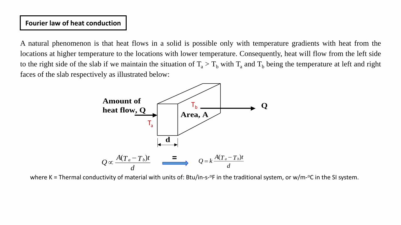
We thus have the thermal force matrix for the 4 nodes as:

4.2

4.2

6.101

100

4.2

4.2

6.1100

100

4

3

22

11

4

3

2

1

h

h

hq

hq

f

f

ff

ff

q

q

q

q

q

The overall structure heat conduction equation: [K]{T} = {q}

4.2

4.2

6.101

100

7375.06.001473.0

6.075.015.00

015.02.16.0

1473.006.07475.0

4

3

2

1

T

T

T

T

(f)

Example 5.1-cont’d Solve for nodal temperatures Example 5.1-cont’d Set thermal forces at the nodes-cont’d

47.595

81.574

38.471

72.629

4.2

4.2

6.101

100

8480.69524.53699.22517.3

9524.55654.63505.20596.3

3699.23505.22728.22913.2

2517.30596.32913.28178.3

4.2

4.2

6.101

100

7375.06.001473.0

6.075.015.00

015.02.16.0

1473.006.07475.01

4

3

2

1

T

T

T

T

(g)

We thus solve for the nodal temperatures to be: T1 = 629.72 oC, T2 = 471.38 oC, T3 = 574.81 oC and T4 = 595.47 oC

Example 5.2 The same Example 13.6 of the textbook on “A First course in the Finite Element Method,” 5th edition by Daryl Logan, published by Cenage Learning, 2012

Problem: “For the 2-D body shown in Figure 13-22, determine the temperature distribution. The temperature at the left side of the body is maintained at 100 oF. The edges on the top and bottom of the body are insulated. There is heat convection from the right side with convective coefficient h = 20 Btu/h-ft2-oF. The free stream temperature is T∞=50 oF. The coefficients of thermal conductivity are Kxx=Kyy=25 Btu/h-ft-oF. The dimensions are shown in the figure. Assume the thickness to be 1 ft.”

h=20

T∞=50 oF

T=100oF

2 ft

2 ft

1

2

3

4

1 2

3 4

5 2 ft

2 ft

Figure 13-22 2-D body subjected to temperature variation and convection

Figure 13-23 Discretized 2-D body of Figure 13-22

Solution: The discretized FE model of the body is shown in Figure 13-23 with 4 elements and 5 nodes. Nodal coordinates are: x1 = 0, y1 = 0 for Node 1 x2 = 2, y2 = 0 for Node 2 x3 = 2, y3 = 2 for Node 3, x4 = 0, y4 = 2 for Node 4, and x5 = 1, y5 = 1 for Node 5 We will formulate the element coefficient matrices for all the 4 elements in Figure 13-23 using the equations (5.25a,b,c) and (5.28)

Example 5.2 – Cont’d

For Element 1: with Nodes 1,2 5

The area 2A is:

22 512512211552 yxyxyxyxyxyxA leads to: A = 1 ft2.

To find the constant coefficients in Equation (5.25a,b,c): From Equation (5.25a):

121

110

20112

251

521

25521

xxc

yyb

yxyxa

From Equation (5.25b):

110

101

01001

512

152

51152

xxc

yyb

yxyxa

From Equation (5.25c):

202

000

00200

123

213

12213

xxc

yyb

yxyxa

Example 5.2 – Cont’d We will use Equation (5.28) to formulate the element coefficient matrix:

2

3

2

332323131

3232

2

2

2

22121

31312121

2

1

2

1

24cbccbbccbb

ccbbcbccbb

ccbbccbbcb

A

kKc (5.28)

255.125.12

5.125.120

5.1205.12

)2()0()2)(1()0)(1()2)(1()0)(1(

)2)(1()0)(1()1()1()1)(1()1)(1(

)2)(1()0)(1()1)(1()1)(1()1(1

14

25

4

22

22

22

2

2

3

2

332323131

3232

2

2

2

22121

31312121

2

1

2

1

2

1

cbccbbccbb

ccbbcbccbb

ccbbccbbcb

A

kKe

Node 1 2 5

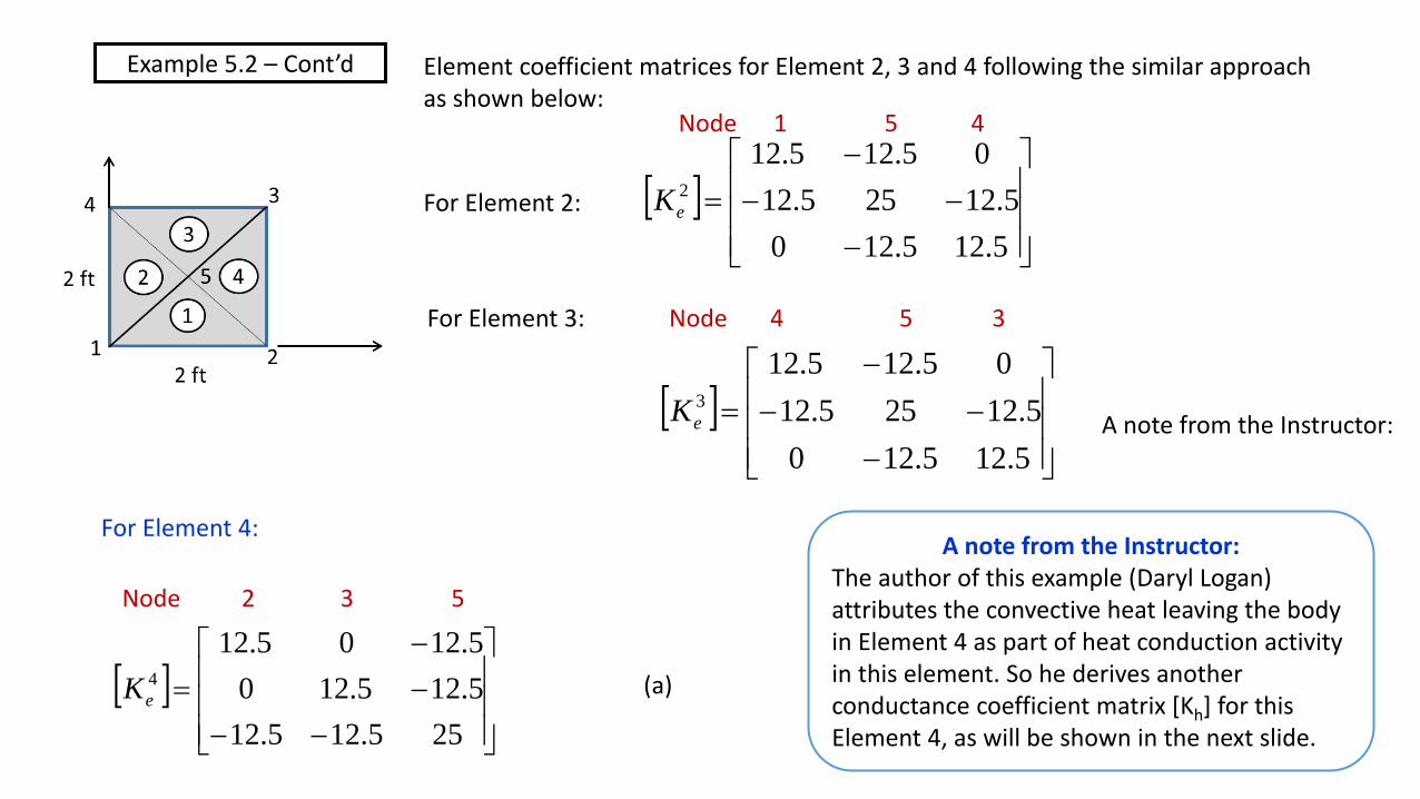
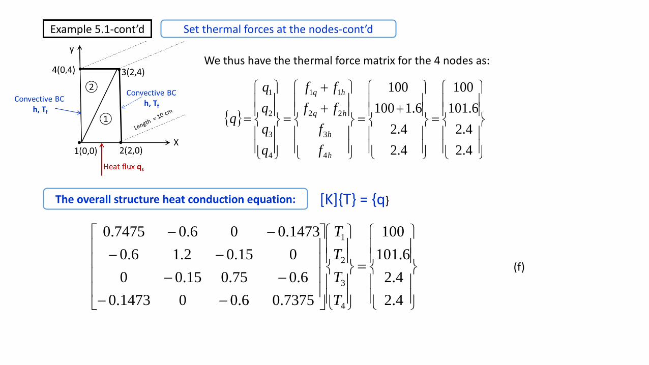
Example 5.2 – Cont’d Element coefficient matrices for Element 2, 3 and 4 following the similar approach as shown below:

5.125.120

5.12255.12

05.125.122

eKFor Element 2:

Node 1 5 4

5.125.120

5.12255.12

05.125.123

eK

For Element 3: Node 4 5 3

255.125.12

5.125.120

5.1205.124

eK

For Element 4:

Node 2 3 5

A note from the Instructor:

A note from the Instructor: The author of this example (Daryl Logan) attributes the convective heat leaving the body in Element 4 as part of heat conduction activity in this element. So he derives another conductance coefficient matrix [Kh] for this Element 4, as will be shown in the next slide.

(a)

Example 5.2 – Cont’d Additional heat conductance matrix for convective heat transfer in Element 4

33 S

mmjmim

mjjjij

mijiiiT

Sh

NNNNNN

NNNNNN

NNNNNN

hdsNNhK

i j

m

h

For the current situation, the side that has convective heat transfer is Side 2-3, we will thus have:

000

021

012

6

)1)(2(204

hK

For the case with convective heat transfer from Edge i-j, the following expression is used:

000

021

012

6

))(( tLhK

ji

h (5.29)

By adding this matrix to the conductance of Element 4 in Equation (a), we obtain the Conductance matrix of Element 4 to be:

255.125.12

5.1283.2567.6

5.1267.683.254

eK

Node 2 3 5

Example 5.2 – Cont’d Assemble the element coefficient matrices for the Overall coefficient matrix by accounting the fact that Node 4 is shred by all 4 elements.

FhBtuK o

/

10025252525

2525000

25033.3867.60

25067.633.380

2500025

(b)

The thermal forces at nodes:

We already know that temperature at Node 1 and 4 are specified to be 100oF The thermal forces across boundary 2-3 of element 4 is:

hBtu

tLTh

f

f

f

f /

0

1000

1000

0

1

1

2

)1)(2)(50(20

0

1

1

2

32

5

3

2

4

Example 5.2 – Cont’d

The overall heat conduction equation becomes:

**

5

4

3

2

1

5000

100

1000

1000

100

10025252525

2525000

25033.3867.60

25067.633.380

2500025

T

T

T

T

T

** = (-25)(100oF)+(-25)(100oF)=-5000oF on the left side of the fifth equation in the left-hand-side of the equation

We may sole the above equations and obtain: T2 = 69.33oF, T3 = 59.33oF and T5 = 84.62oF with specified T1=T4 = 100oF

Summary on Heat Conduction Analysis of Plane Structures by FE Method

1) An overview of heat conduction in 3-D solids was presented in this Chapter with heat conduction equation for the induced temperature distributions in the solids by the sources of: (a) heat generation by the solid, (b) the prescribed surface temperature, (c) specified heat flux across the boundary surfaces, and (d) the convective heat across the boundary surfaces. 2) Finite element formulation of heat conduction in solids is derived using the Galerkin method due to the fact that heat conduction in solids can e described by the heat conduction equations with prescribed boundary conditions by mathematical expressions. 3) Finite element formulations begin with the derivation of interpolation functions [N} = {Ni Nj Nm} for triangular plane elements with Nodes i, j and m. These functions relate the “element temperatures” and the “nodal temperatures.” 4) The interpolation functions for the FE analysis were derive on the basis of linear polynomial function for the temperature variations in the element. 5) Special FE formulations of the aforementioned boundary conditions were presented.

6) This chapter only presents the FE formulation for steady-state heat conduction in solids of plane geometry.

Documents

ME 160 Introduction to Finite Element Method Chapter 5 ... Conduc.pdf · Finite Element Analysis in Heat Conduction Analysis of Solid Structures ... and h is the heat transfer coefficient