ME 415 Energy Systems Design

Tutorial

COURSE MATERIAL

This is a classic thermal systems design course. It is application intensive and covers flow in pipes and piping systems, pumps and pumping systems, heat exchangers and heat exchanger design, and thermal system simulation.

APPLICATION THROUGH EXCEL

The ME 415 Add-In offers several unique ‘user-defined’ functions for application of course material in the Excel environment. As a result, students are able to solve complex problems through elimination of cumbersome hand calculations or reading of charts and graphs.

APPLICATION THROUGH EXCEL

These ‘user-defined’ functions are utilized in the Excel Spreadsheet.

The functions can be invoked by several methods. Call directly from the cell

Requires known function name and argument constraints (specific units, range sizes, etc.)

Call from the user ribbon (Excel 2007) Provides function descriptions and input boxes

DIRECT CELL CALL METHOD This method requires the user to highlight

desired cell(s) for output and type =‘Function Name(Arg1,Arg2,…)’ For example, we desire to know the Nusselt

number for turbulent flow in a tube.This method requires knowing what arguments the function needs to compute the desired output.

Direct cell call method becomes useful when user has gained experience with a specific function or group of functions.

USER RIBBON CALL METHOD This method uses the ‘user ribbon’ and the

‘Insert –Function’ button located at the top of the Excel 2007 window. Advantages of this method are function lists and

descriptions that provide details on each argument’s requirements .

Highlight cell(s) for desired output and select the formulas tab on the user-ribbon as seen on following slide.

Then click either ‘Insert-Function’ button

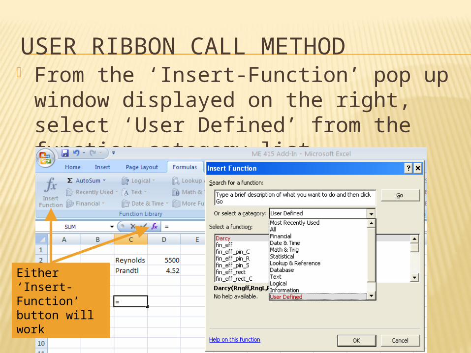
USER RIBBON CALL METHOD From the ‘Insert-Function’ pop up

window displayed on the right, select ‘User Defined’ from the function category list.

Either ‘Insert-Function’ button will work

USER RIBBON CALL METHOD User can select the correct function by scrolling

through each function and its description. Once function is selected, spaces are provided for each argument. Some arguments can be optional such as the ‘Quiet’ argument on the ‘NuDTurbTube’ function.

ME 415 ADD-IN FEATURES

The ME 415 Add-In provides tools for several special design calculations. Heat Transfer Fin Efficiency Heat Exchanger Effectiveness-Number of Transfer

Units (NTU) Method Pump Performance Correction for Viscous Fluids Hardy-Cross Flow and Hazen-Williams Head Loss

Analysis Friction Factor Calculator (Swamee-Jain and

Churchill) Nusselt Number

FIN EFFICIENCY

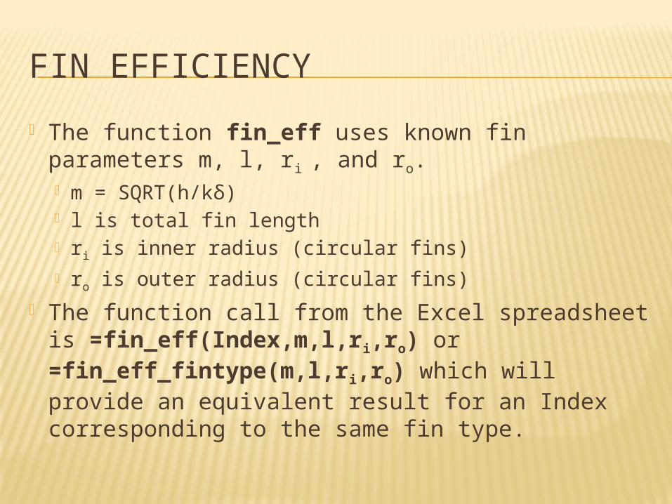
The function fin_eff uses known fin parameters m, l, ri , and ro. m = SQRT(h/kδ) l is total fin length ri is inner radius (circular fins) ro is outer radius (circular fins)

The function call from the Excel spreadsheet is =fin_eff(Index,m,l,ri,ro) or =fin_eff_fintype(m,l,ri,ro) which will provide an equivalent result for an Index corresponding to the same fin type.

FIN EFFICIENCY Study of finned surfaces in heat exchanger

design requires analysis of fin efficiency. Calculation of fin efficiency can become

cumbersome with complex fin geometries. With known fin dimensions, the ‘user-defined’

function fin_eff readily calculates fin efficiency.

From calculation of fin efficiency, further analysis of finned surface properties such as total surface effectiveness can be easily determined.

FIN EFFICIENCY When using the =fin_eff_fintype function call, the following

function names should be used for each specific fin geometry. Straight Rectangular Fins

=fin_eff_rect(m, l) Straight Triangular Fins

=fin_eff_tri(m, l) Circular Rectangular Fins

=fin_eff_rect_c(m, l, ri, ro) ri and ro are required arguments here

Rectangular Spines (Circular cross-section) “Round Pin Fin” =fin_eff_pin_R(m, l)

Rectangular Spines (Square cross-section) “Square Pin Fin” m = Sqrt(2*h/k/δ) =fin_eff_pin_S(m,l)

Triangular Spines (Circular “Cone” cross-section) “Cone Pin Fin” =fin_eff_pin_C(m,l)

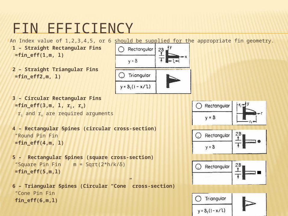
FIN EFFICIENCY An Index value of 1,2,3,4,5, or 6 should be supplied for the appropriate fin geometry.

1 – Straight Rectangular Fins =fin_eff(1,m, l)

2 – Straight Triangular Fins =fin_eff2,m, l)

3 – Circular Rectangular Fins =fin_eff(3,m, l, ri, ro)

ri and ro are required arguments

4 – Rectangular Spines (circular cross-section) “Round Pin Fin” =fin_eff(4,m, l)

5 - Rectangular Spines (square cross-section) “Square Pin Fin” m = Sqrt(2*h/k/δ) =fin_eff(5,m,l)

6 – Triangular Spines (Circular “Cone” cross-section) “Cone Pin Fin” fin_eff(6,m,l)

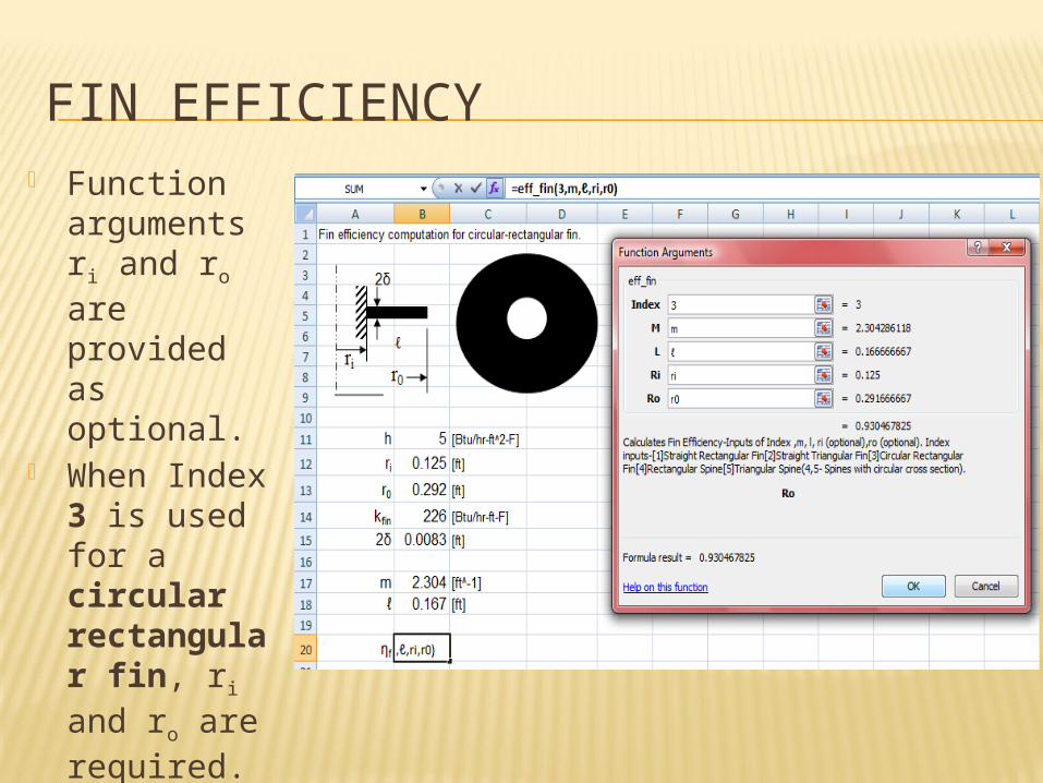
FIN EFFICIENCY Function

arguments ri and ro are provided as optional.

When Index 3 is used for a circular rectangular fin, ri and ro are required. Otherwise, they should not be supplied.

NTU METHOD The function calls from the Excel spreadsheet are =Hx_eff(

Index,NTU,Cmin ,Cmax ,Passes) and =Hx_NTU( Index,eff, Cmin ,Cmax ,Passes).

The function Hx_eff uses known parameters NTU, Cmin, Cmax, and No. of Passes to calculate heat exchanger effectiveness. NTU=UA/Cmin. Cmin is the smaller of the two capacities Ch and Cc. Cmax is the larger of the two capacities Ch and Cc. Passes is an optional argument (specific to certain heat exchanger

types). The function Hx_NTU uses known parameters effectiveness,

Cmin, Cmax, and No. of Passes to calculate NTU. Where Cmin, Cmax, and Passes are same as above.

NTU METHOD

Heat exchanger analysis where only inlet conditions are known uses the Number of Transfer Units (NTU) Method to determine heat exchanger effectiveness.

Effectiveness – NTU relations for some heat exchanger types require iterative calculation which is simplified by ‘user-defined’ functions Hx_eff and Hx_NTU.

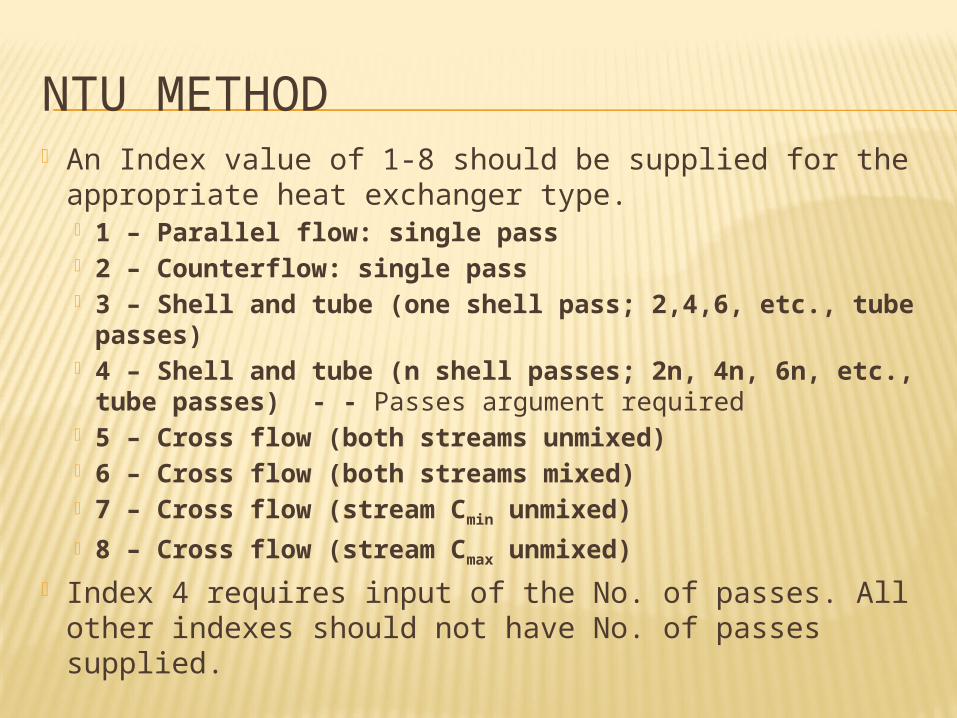
NTU METHOD An Index value of 1-8 should be supplied for the

appropriate heat exchanger type. 1 – Parallel flow: single pass 2 – Counterflow: single pass 3 – Shell and tube (one shell pass; 2,4,6, etc., tube

passes) 4 – Shell and tube (n shell passes; 2n, 4n, 6n, etc.,

tube passes) - - Passes argument required 5 – Cross flow (both streams unmixed) 6 – Cross flow (both streams mixed) 7 – Cross flow (stream Cmin unmixed) 8 – Cross flow (stream Cmax unmixed)

Index 4 requires input of the No. of passes. All other indexes should not have No. of passes supplied.

NTU METHOD The direct cell call method uses

=Hx_eff( Index,NTU,Cmin ,Cmax ,Passes) and =Hx_NTU( Index,eff, Cmin ,Cmax ,Passes).

The ‘user-ribbon’ call method is shown in the figure below.

VISCOUS PUMP

The function calls from the Excel spreadsheet are =Vis_pump_QHE(QHE_Matrix,Vis) and =Vis_pump_CF(QBE, HBE, Vis).

The function Vis_pump_QHE uses a pre-calculated QHE matrix and viscosity of the pumping fluid to provide corresponding flow and head values for the high viscosity fluid. The user can then generate (plot) a new pump curve with the supplied output.

The function Vis_pump_CF uses known best efficiency point (BEP) flow and head values along with the viscosity of the pumping fluid to provide correction factors that ‘correct’ the pump curve data. The user can multiply these correction factors with original pump data to find corresponding flow and head values for the high viscosity fluid.

VISCOUS PUMP Because pump performance is greatly affected

by highly viscous fluids, a correction method must be used to estimate performance when manufacturer’s data is not available.

These pump corrections can be found from charts but is simplified through ‘user-defined’ functions Vis_pump_QHE and Vis_pump_CF.

With the known best efficiency point (BEP) of a specific pump, the correction factors for efficiency, flow, Head0.6Q, Head0.8Q, Head1.0Q, and Head1.2Q can be found. Both ‘user-defined’ functions use a BEP to calculate and output the new data for a high viscosity pumping fluid.

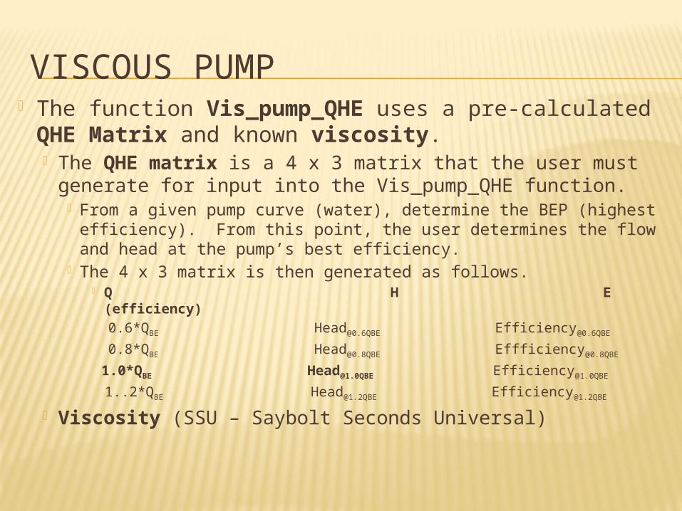
VISCOUS PUMP The function Vis_pump_QHE uses a pre-

calculated QHE Matrix and known viscosity. The QHE matrix is a 4 x 3 matrix that the user

must generate for input into the Vis_pump_QHE function.

From a given pump curve (water), determine the BEP (highest efficiency). From this point, the user determines the flow and head at the pump’s best efficiency.

The 4 x 3 matrix is then generated as follows. Q H E (efficiency) 0.6*QBE Head@0.6QBE Efficiency@0.6QBE

0.8*QBE Head@0.8QBE Effficiency@0.8QBE

1.0*QBE Head@1.0QBE Efficiency@1.0QBE

1..2*QBE Head@1.2QBE Efficiency@1.2QBE

Viscosity (SSU – Saybolt Seconds Universal)

VISCOUS PUMP

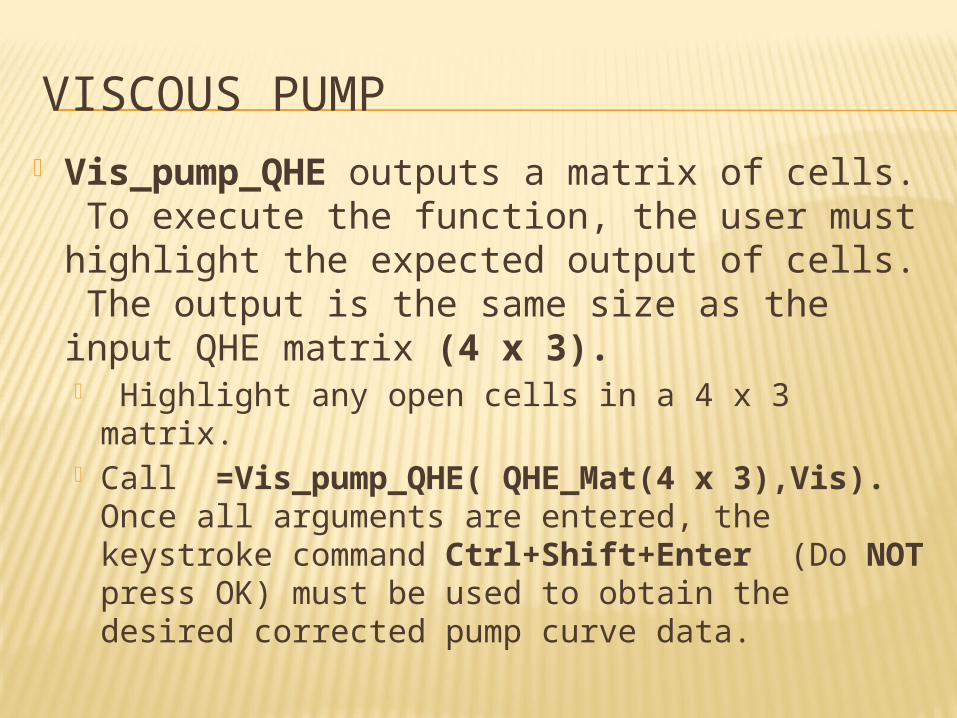
Vis_pump_QHE outputs a matrix of cells. To execute the function, the user must highlight the expected output of cells. The output is the same size as the input QHE matrix (4 x 3). Highlight any open cells in a 4 x 3 matrix. Call =Vis_pump_QHE( QHE_Mat(4 x

3),Vis). Once all arguments are entered, the keystroke command Ctrl+Shift+Enter (Do NOT press OK) must be used to obtain the desired corrected pump curve data.

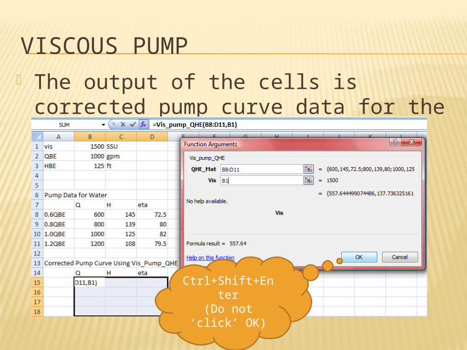
VISCOUS PUMP The output of the cells is corrected

pump curve data for the high viscosity fluid.

Ctrl+Shift+Enter

(Do not ‘click’ OK)

VISCOUS PUMP The function Vis_pump_CF uses known BEP

arguments flow (QBE), head (HBE), and viscosity. Flow (GPM) Head (‘ft’) Viscosity (SSU – Saybolt Seconds Universal)

Vis_pump_CF outputs an array of cells. To execute the function, the user must highlight the expected array of six cells in any column and call =Vis_pump_CF( Flow,Head,Vis). Once all arguments are entered, the keystroke command Ctrl+Shift+Enter (Do NOT press OK) must be used to obtain the desired correction factors.

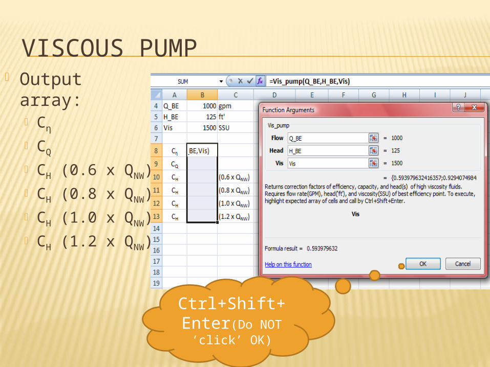
VISCOUS PUMP Output array:

Cη

CQ

CH (0.6 x QNW) CH (0.8 x QNW) CH (1.0 x QNW) CH (1.2 x QNW)

Ctrl+Shift+Enter(Do NOT ‘click’

OK)

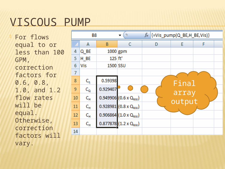
VISCOUS PUMP For flows

equal to or less than 100 GPM, correction factors for 0.6, 0.8, 1.0, and 1.2 flow rates will be equal. Otherwise, correction factors will vary.

Final array

output

HARDY-CROSS ANALYSIS

The function calls from the Excel spreadsheet are =Hardy_Darcy(RngL,RngD,RngQ,RngN,RngE,rho,v

is) =Darcy(RngL,RngD,RngQ,RngE,rho,vis)and =Hardy_Hazen(RngL,RngD,RngQ,RngN,RngC,tol,k

1) =HazenWill(RngL,RngD,RngQ,k1,RngC)

Darcy-Weisbach and Hazen-Williams are two methods for calculating head loss through pipes. They use unique parameters to determine friction and head-loss through piping systems. With appropriate input arguments, these two methods will provide approximately the same solution.

HARDY-CROSS ANALYSIS Hardy-Cross formulation is an iterative

method for obtaining the steady-state solution for any generalized series-parallel flow network. It can be systematically applied to any fluid flow network.

While Hardy-Cross flow values can be obtained using ‘solver’ in Excel, an alternative method that employs ‘user-defined’ functions Hardy_Darcy and Hardy_Hazen supplies the same solution.

HARDY-CROSS AND DARCY-WEISBACH

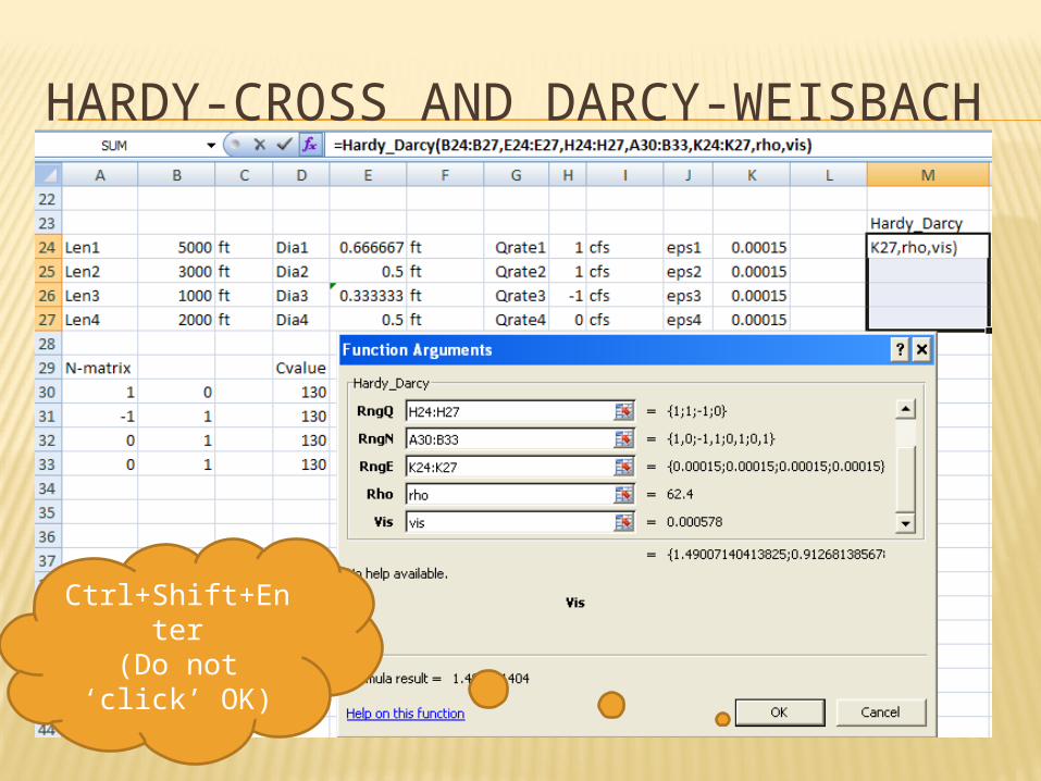
The function Hardy _Darcy uses system geometry, initial guesses for line flow rates, loop-node analysis, pipe roughness, density, and dynamic viscosity to determine flow through the system.

Corresponding to the number of pipes in the system, the user should supply a range of lengths (RngL), diameters (RngD), initial flow guesses (RngQ), and epsilon values coefficients (RngE). The user also supplies a n-connection matrix (RngN), a density, and a dynamic viscosity.

The function call from the Excel spreadsheet is =Hardy_Darcy(RngL,RngD,RngQ,RngN,RngE,rho,vis).

HARDY-CROSS AND DARCY-WEISBACH The user must input a rho (density) and vis

(dynamic viscosity). Typical units for each are lbm/ft3 and ft2/sec, respectively, when units of Q are ft3/sec.

Hardy_Darcy outputs an array of cells. To execute the function, the user must highlight the expected array of cells (No. of pipes in system) in any column and call =Hardy_Darcy(RngL,RngD,RngQ,RngN,RngE,rho,vis). Once all arguments are entered, the keystroke command Ctrl+Shift+Enter (Do NOT press OK) must be used to obtain the desired Hardy flow values.

HARDY-CROSS AND DARCY-WEISBACH

Ctrl+Shift+Enter

(Do not ‘click’ OK)

HARDY-CROSS AND DARCY-WEISBACH

The final array output Hardy _Darcy flow values are shown above. Darcy-Weisbach head loss values through each pipe can then be found with these known flow rates.

Final array

output

HARDY-CROSS AND DARCY-WEISBACH The ‘user-defined’ function Darcy uses the same system geometry and the calculated Hardy_Darcy flow values to find the head loss through each pipe.

The function call from the Excel spreadsheet is =Darcy(RngL,RngD,RngQ,RngE,rho,vis).

Since the Darcy function also uses range inputs, the keystroke command Ctrl+Shift+Enter must again be used to obtain the expected array Darcy head loss values.

HARDY-CROSS AND DARCY-WEISBACH

RngQ uses new

Hardy_Darcy flow values

HARDY-CROSS AND HAZEN-WILLIAMS

The function Hardy _Hazen uses system geometry, initial guesses for line flow rates, and loop-node analysis to determine flow through the system.

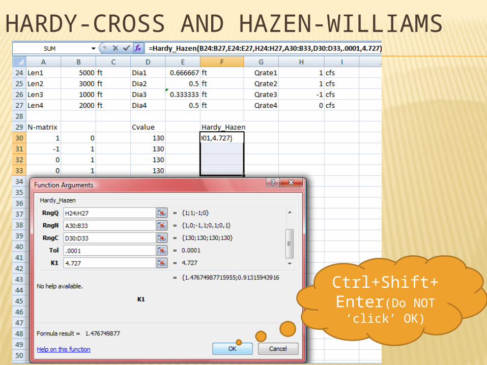
Corresponding to the number of pipes in the system, the user should supply a range of lengths (RngL), diameters (RngD), initial flow guesses (RngQ), and Hazen-Williams coefficients (RngC). The user also supplies a n-connection matrix (RngN), a tolerance value (tol), and a K1 value (k1).

The function call from the Excel spreadsheet is =Hardy_Hazen(RngL,RngD,RngQ,RngN,RngC,tol,k1).

HARDY-CROSS AND HAZEN-WILLIAMS Typical values for tol and k1 are .0001 and 4.727

respectively when units of Q are ft3/sec. Hardy_Hazen outputs an array of cells. To

execute the function, the user must highlight the expected array of cells (No. of pipes in system) in any column and call =Hardy(RngL,RngD,RngQ,RngN,RngC,tol,k1). Once all arguments are entered, the keystroke command Ctrl+Shift+Enter (Do NOT press OK) must be used to obtain the desired Hardy flow values.

HARDY-CROSS AND HAZEN-WILLIAMS

Ctrl+Shift+Enter(Do NOT ‘click’

OK)

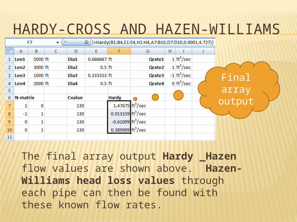
HARDY-CROSS AND HAZEN-WILLIAMS

The final array output Hardy _Hazen flow values are shown above. Hazen-Williams head loss values through each pipe can then be found with these known flow rates.

Final array

output

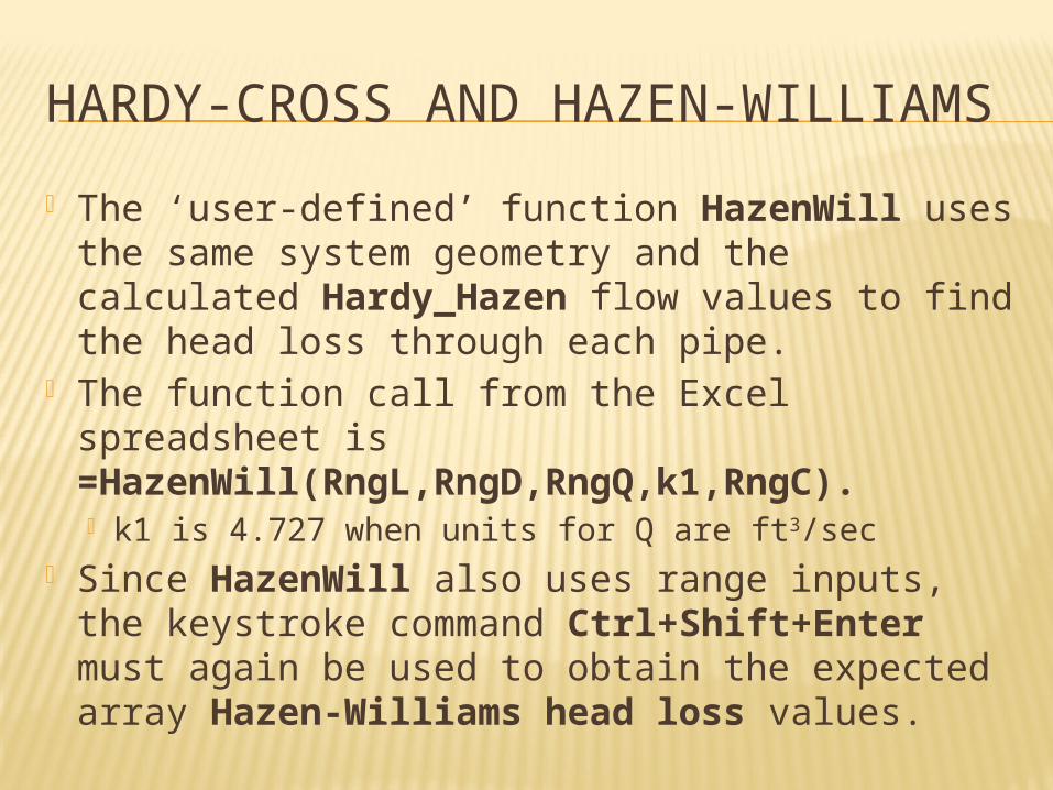
HARDY-CROSS AND HAZEN-WILLIAMS The ‘user-defined’ function HazenWill uses

the same system geometry and the calculated Hardy_Hazen flow values to find the head loss through each pipe.

The function call from the Excel spreadsheet is =HazenWill(RngL,RngD,RngQ,k1,RngC). k1 is 4.727 when units for Q are ft3/sec

Since HazenWill also uses range inputs, the keystroke command Ctrl+Shift+Enter must again be used to obtain the expected array Hazen-Williams head loss values.

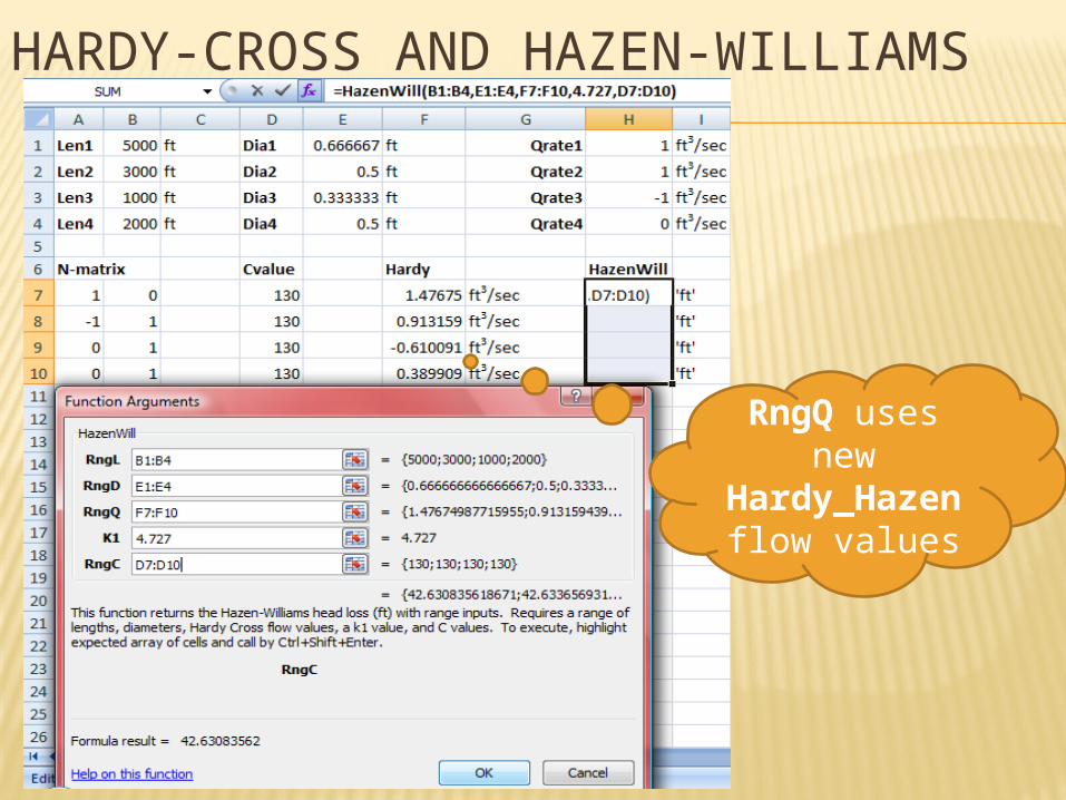
HARDY-CROSS AND HAZEN-WILLIAMS

RngQ uses new

Hardy_Hazen flow values

FRICTION FACTOR

The function calls from the Excel spreadsheet are =fric_Swamee(Eps_Dia, ReD) =fric_Churchill(Eps_Dia, ReD)

Eps_Dia is the relative roughness = ε/D ReD is the Reynolds number = ρ*V*D/μ

Swamee-Jain and Churchill are two methods for calculating friction factors, a value necessary for calculating head loss through piping. Each function must be used with caution, as they each represent friction factors for different flow regions.

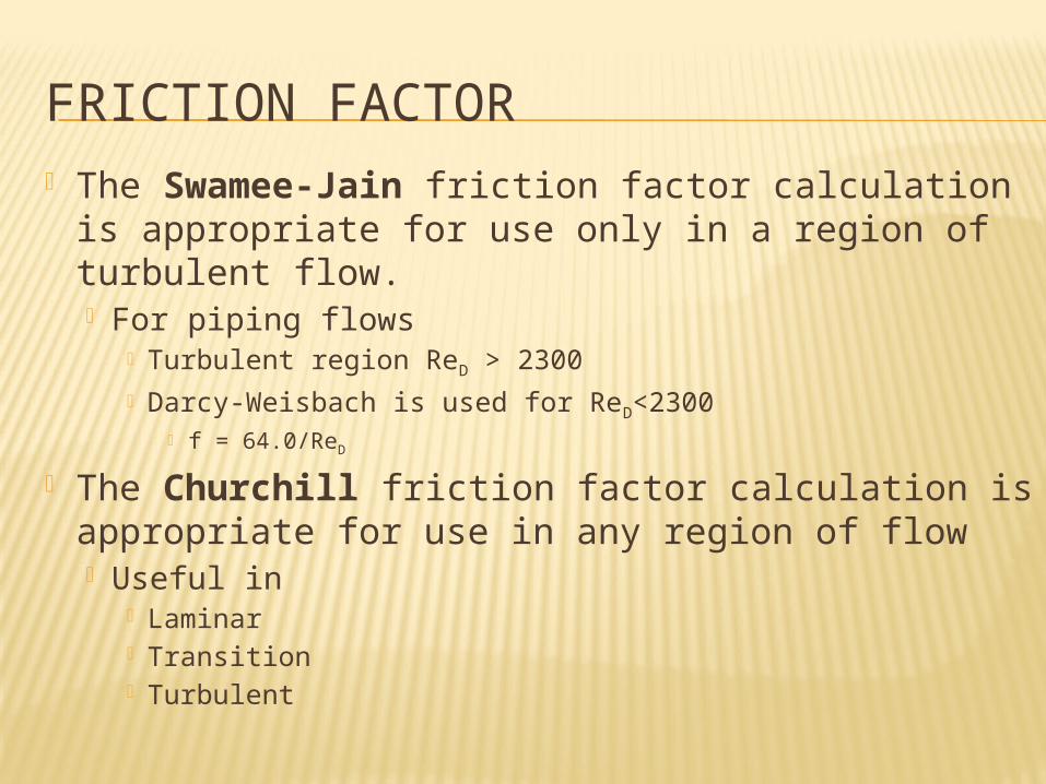
FRICTION FACTOR The Swamee-Jain friction factor calculation is

appropriate for use only in a region of turbulent flow. For piping flows

Turbulent region ReD > 2300 Darcy-Weisbach is used for ReD<2300

f = 64.0/ReD

The Churchill friction factor calculation is appropriate for use in any region of flow Useful in

Laminar Transition Turbulent

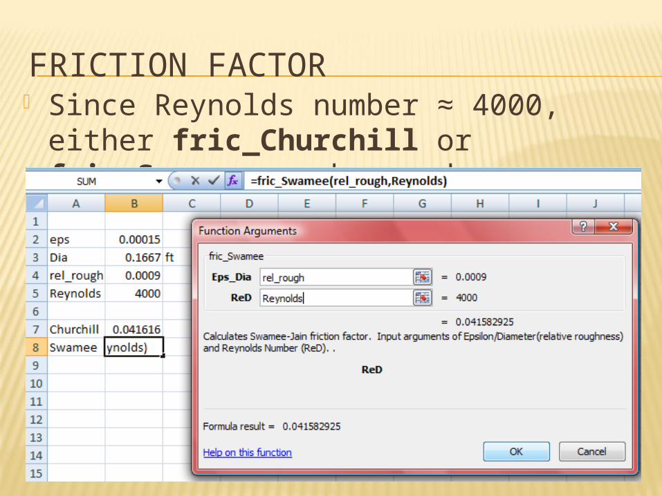
FRICTION FACTOR Since Reynolds number ≈ 4000, either

fric_Churchill or fric_Swamee can be used

NUSSELT NUMBERS

Optional Inputs in italics NuxPlate(Re, Pr, Rexc, Quiet) NuBarPlate(Re, Pr, Rexc, Quiet) NuDBarCyl(Re, Pr, Quiet) NuDBarSphere(Re, Pr, mu_mus, Quiet) NuDBarTubes(Re, Pr, St_D, Sl_D, Aligned, Nl, Quiet)

NuDBarZTubes(Re, Pr, Prs, St_Sl, Aligned, Nl, Quiet)

NuDBarLamTube(Re, Pr, D_L, Thermal, mu_mus, Quiet)

NuDTurbTube(Re, Pr, Quiet) NuDLiqMetals (Re, Pr, UniformT, Quiet)

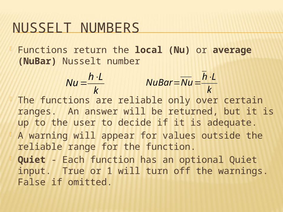
NUSSELT NUMBERS Functions return the local (Nu) or average

(NuBar) Nusselt number

The functions are reliable only over certain ranges. An answer will be returned, but it is up to the user to decide if it is adequate.

A warning will appear for values outside the reliable range for the function.

Quiet - Each function has an optional Quiet input. True or 1 will turn off the warnings. False if omitted.

k

LhNu

k

LhNuNuBar

NUSSELT: FLAT PLATE, LOCAL NuxPlate(Re, Pr, Rexc, Quiet) Returns the local Nusselt number at x Inputs based on the film temperature, Tf = (Ts+T∞)/2

Re - Reynolds number, Rex = V x / ν Pr - Prandtl number, Pr = Cp μ / k = ν / α Rexc - Critical Reynolds number. Reynolds number at transition

point from laminar to turbulent. If Re < Rexc, then laminar calculation. Otherwise, the calculation is for turbulent flow. If omitted, Recx = 5 X 105

Ranges For laminar, Pr ≥ 0.6 For turbulent, Rex ≤ 108, 0.6 ≤ Pr ≤ 60

TurbulentLaminar

x Ts

V, T∞

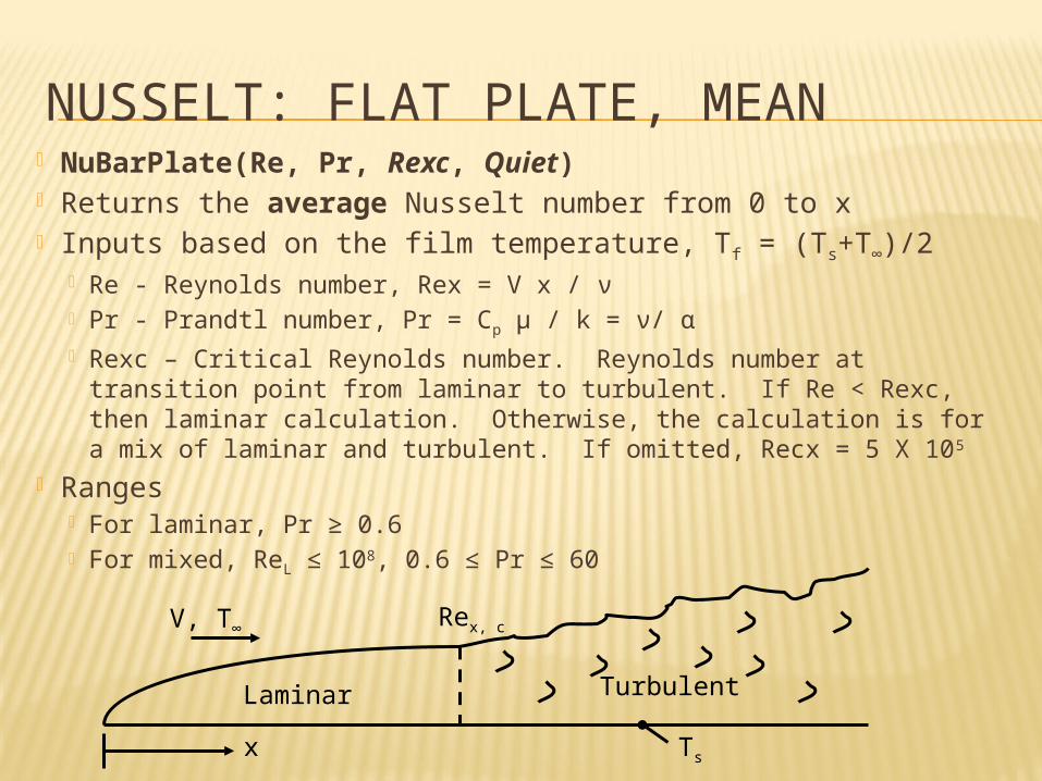
NUSSELT: FLAT PLATE, MEAN NuBarPlate(Re, Pr, Rexc, Quiet) Returns the average Nusselt number from 0 to x Inputs based on the film temperature, Tf = (Ts+T∞)/2

Re - Reynolds number, Rex = V x / ν Pr - Prandtl number, Pr = Cp μ / k = ν/ α Rexc – Critical Reynolds number. Reynolds number at transition

point from laminar to turbulent. If Re < Rexc, then laminar calculation. Otherwise, the calculation is for a mix of laminar and turbulent. If omitted, Recx = 5 X 105

Ranges For laminar, Pr ≥ 0.6 For mixed, ReL ≤ 108, 0.6 ≤ Pr ≤ 60

TurbulentLaminar

x Ts

V, T∞ Rex, c

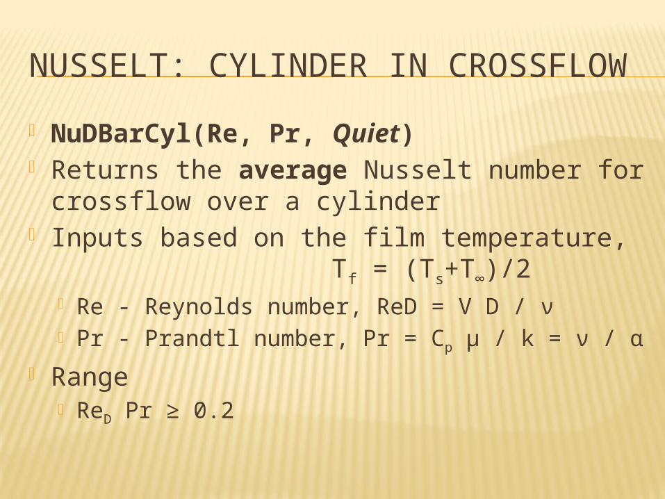
NUSSELT: CYLINDER IN CROSSFLOW

NuDBarCyl(Re, Pr, Quiet) Returns the average Nusselt number for

crossflow over a cylinder Inputs based on the film temperature,

Tf = (Ts+T∞)/2 Re - Reynolds number, ReD = V D / ν Pr - Prandtl number, Pr = Cp μ / k = ν / α

Range ReD Pr ≥ 0.2

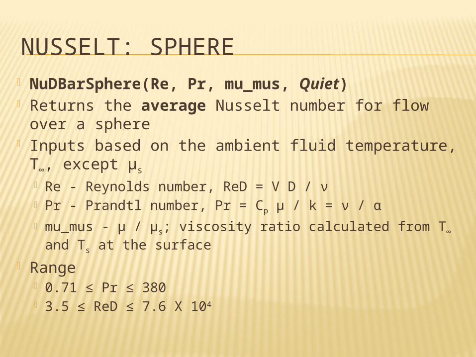
NUSSELT: SPHERE NuDBarSphere(Re, Pr, mu_mus, Quiet) Returns the average Nusselt number for flow over a

sphere Inputs based on the ambient fluid temperature, T∞,

except μs

Re - Reynolds number, ReD = V D / ν Pr - Prandtl number, Pr = Cp μ / k = ν / α mu_mus - μ / μs; viscosity ratio calculated from T∞ and Ts at

the surface Range

0.71 ≤ Pr ≤ 380 3.5 ≤ ReD ≤ 7.6 X 104

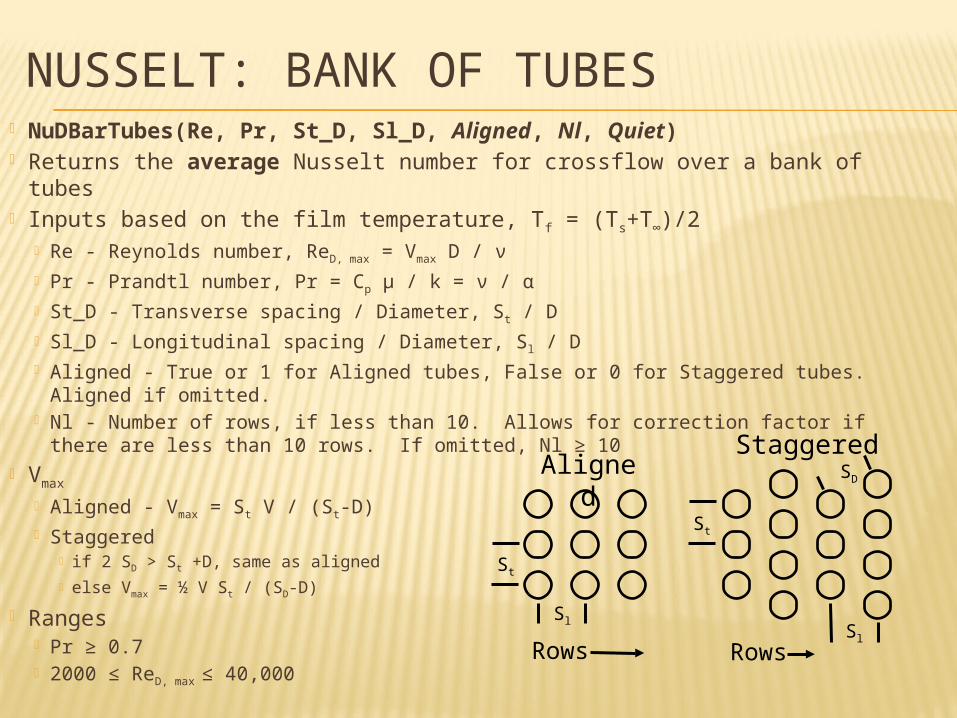
NUSSELT: BANK OF TUBES NuDBarTubes(Re, Pr, St_D, Sl_D, Aligned, Nl, Quiet) Returns the average Nusselt number for crossflow over a bank of tubes Inputs based on the film temperature, Tf = (Ts+T∞)/2

Re - Reynolds number, ReD, max = Vmax D / ν Pr - Prandtl number, Pr = Cp μ / k = ν / α St_D - Transverse spacing / Diameter, St / D Sl_D - Longitudinal spacing / Diameter, Sl / D Aligned - True or 1 for Aligned tubes, False or 0 for Staggered tubes. Aligned if

omitted. Nl - Number of rows, if less than 10. Allows for correction factor if there are less

than 10 rows. If omitted, Nl ≥ 10 Vmax

Aligned - Vmax = St V / (St-D) Staggered

if 2 SD > St +D, same as aligned else Vmax = ½ V St / (SD-D)

Ranges Pr ≥ 0.7 2000 ≤ ReD, max ≤ 40,000

AlignedStaggered

Rows Rows

St

SlSl

St

SD

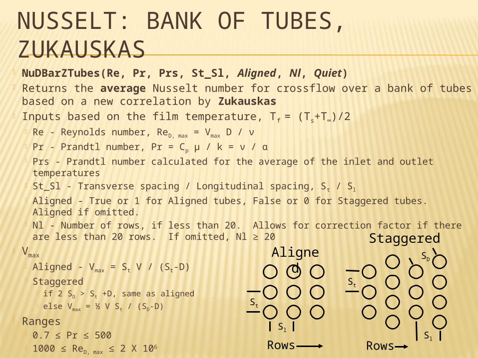
NUSSELT: BANK OF TUBES, ZUKAUSKAS

NuDBarZTubes(Re, Pr, Prs, St_Sl, Aligned, Nl, Quiet) Returns the average Nusselt number for crossflow over a bank of tubes

based on a new correlation by Zukauskas Inputs based on the film temperature, Tf = (Ts+T∞)/2

Re - Reynolds number, ReD, max = Vmax D / ν Pr - Prandtl number, Pr = Cp μ / k = ν / α Prs - Prandtl number calculated for the average of the inlet and outlet temperatures St_Sl - Transverse spacing / Longitudinal spacing, St / Sl

Aligned - True or 1 for Aligned tubes, False or 0 for Staggered tubes. Aligned if omitted.

Nl - Number of rows, if less than 20. Allows for correction factor if there are less than 20 rows. If omitted, Nl ≥ 20

Vmax

Aligned - Vmax = St V / (St-D) Staggered

if 2 SD > St +D, same as aligned else Vmax = ½ V St / (SD-D)

Ranges 0.7 ≤ Pr ≤ 500 1000 ≤ ReD, max ≤ 2 X 106

AlignedStaggered

Rows Rows

St

SlSl

St

SD

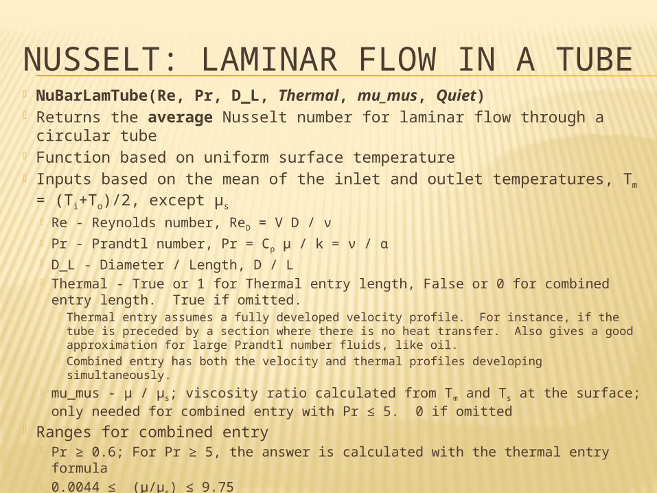
NUSSELT: LAMINAR FLOW IN A TUBE NuBarLamTube(Re, Pr, D_L, Thermal, mu_mus, Quiet) Returns the average Nusselt number for laminar flow through a

circular tube Function based on uniform surface temperature Inputs based on the mean of the inlet and outlet temperatures, Tm =

(Ti+To)/2, except μs

Re - Reynolds number, ReD = V D / ν Pr - Prandtl number, Pr = Cp μ / k = ν / α D_L - Diameter / Length, D / L Thermal - True or 1 for Thermal entry length, False or 0 for combined entry

length. True if omitted. Thermal entry assumes a fully developed velocity profile. For instance, if the tube is

preceded by a section where there is no heat transfer. Also gives a good approximation for large Prandtl number fluids, like oil.

Combined entry has both the velocity and thermal profiles developing simultaneously. mu_mus - μ / μs; viscosity ratio calculated from Tm and Ts at the surface; only

needed for combined entry with Pr ≤ 5. 0 if omitted Ranges for combined entry

Pr ≥ 0.6; For Pr ≥ 5, the answer is calculated with the thermal entry formula 0.0044 ≤ (μ/μs) ≤ 9.75

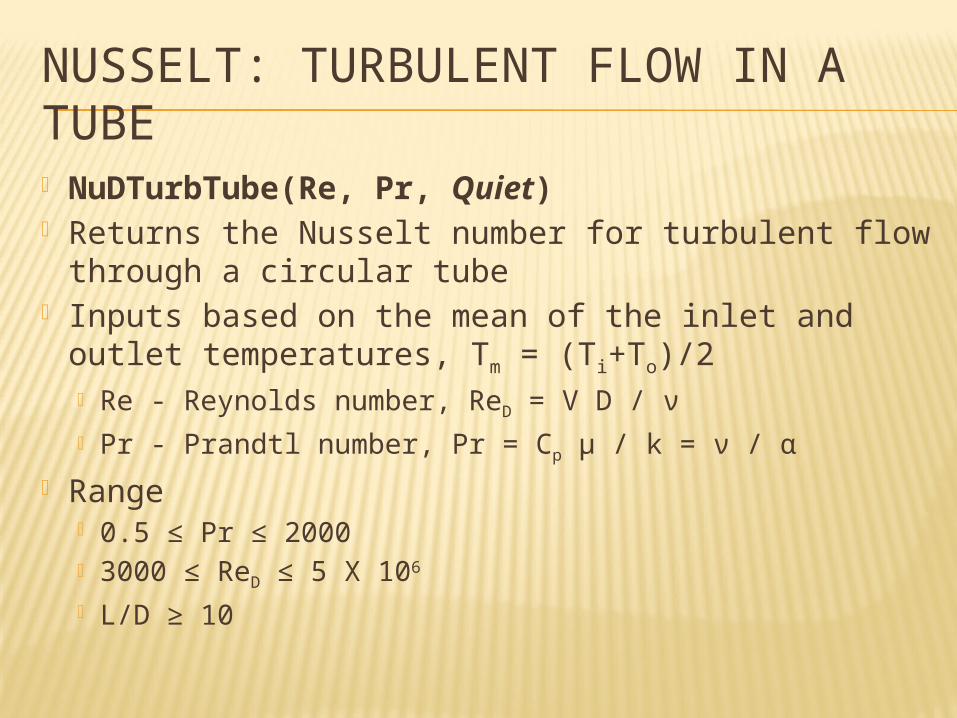
NUSSELT: TURBULENT FLOW IN A TUBE NuDTurbTube(Re, Pr, Quiet) Returns the Nusselt number for turbulent flow

through a circular tube Inputs based on the mean of the inlet and outlet

temperatures, Tm = (Ti+To)/2 Re - Reynolds number, ReD = V D / ν Pr - Prandtl number, Pr = Cp μ / k = ν / α

Range 0.5 ≤ Pr ≤ 2000 3000 ≤ ReD ≤ 5 X 106

L/D ≥ 10

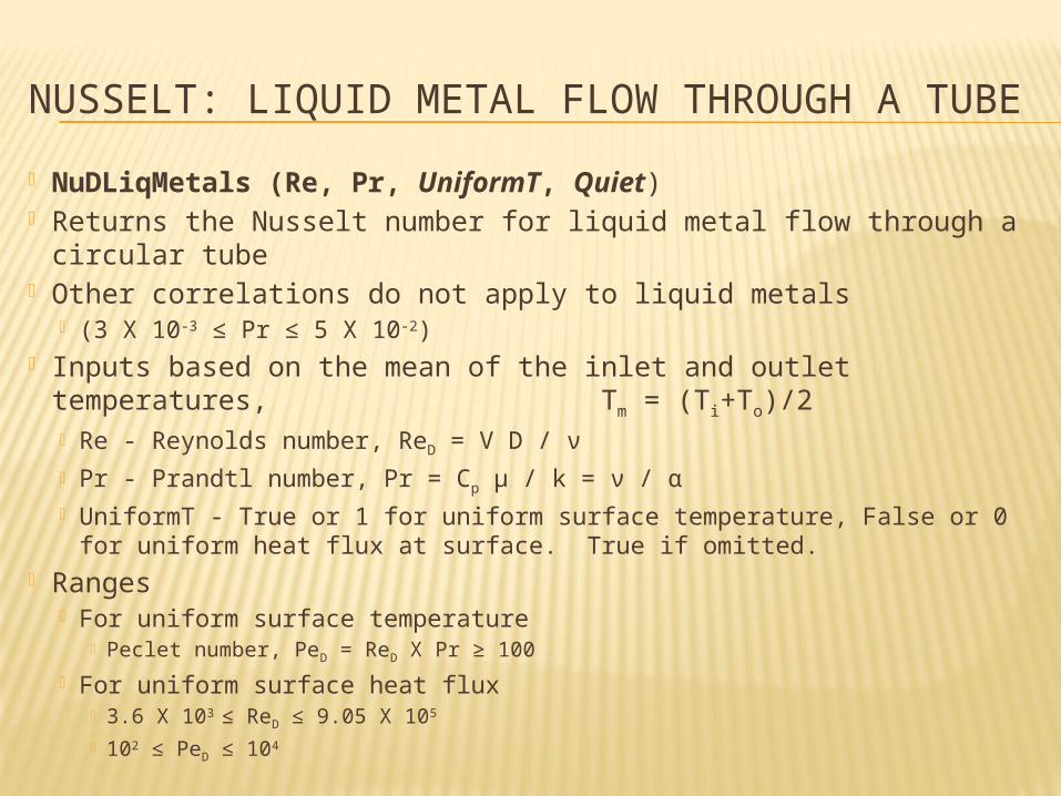
NUSSELT: LIQUID METAL FLOW THROUGH A TUBE NuDLiqMetals (Re, Pr, UniformT, Quiet) Returns the Nusselt number for liquid metal flow through a circular

tube Other correlations do not apply to liquid metals

(3 X 10-3 ≤ Pr ≤ 5 X 10-2) Inputs based on the mean of the inlet and outlet temperatures,

Tm = (Ti+To)/2 Re - Reynolds number, ReD = V D / ν Pr - Prandtl number, Pr = Cp μ / k = ν / α UniformT - True or 1 for uniform surface temperature, False or 0 for

uniform heat flux at surface. True if omitted. Ranges

For uniform surface temperature Peclet number, PeD = ReD X Pr ≥ 100

For uniform surface heat flux 3.6 X 103 ≤ ReD ≤ 9.05 X 105

102 ≤ PeD ≤ 104