Embed Size (px)
DESCRIPTION
A comprehensive report on the design of an oil pump-jack and how it can be made more efficiently in relation to energy and cost.
Citation preview
Oil Pumpjack
Team Members:
Joe Gammie Greg Jones
Jennifer LaMere Jeremiah Roberts
ME 3180 – Machine Design
Dr. Raghu Pucha
The George W. Woodruff School of Mechanical Engineering Georgia Institute of Technology
Atlanta, GA 30332-0405

2
Table of Contents
1) Project Proposal 2) Mechanical System and Design Goals 3) Mechanical Elements
i) Bolted Joints – Joe Gammie ii) Welded Joints – Greg Jones iii) Wire Rope – Jennifer LaMere iv) Shafts – Jeremiah Roberts v) Bearing – Group Design
4) Studies and Design Optimizations i) Bolted Joints – Joe Gammie ii) Welded Joints – Greg Jones iii) Wire Rope – Jennifer LaMere iv) Shafts – Jeremiah Roberts v) Bearing – Group Design
5) Design Goals and Conclusion 6) Appendix

3
Part 1:
Project Proposal

4
Project Proposal
Pumpjack Introduction and Design
An oil pumpjack is used to remove liquids, like water or oil, from underground
reserves. Based on the size of the machine, it can extract 5 to 40 liters of liquid with
each pump, pulling against approximately 600 bars of pressure.
Figure 1.1: Pumpjack Components
Figure 1.1 displays the large number of components that compose an oil
pumpjack. In order to limit the scope of the project, the team selected elements that
carry the most loads. Thus the gearbox and rotator on the left of the image were elided.
The group focused on the resisting force through the wire rope and the components that
support this weight and the weight of the components. In Table 1.1, the elements were
divided among the group such that each member had one element individually and one
element to work on as a team.
J. Gammie G. Jones J. LaMere J. Roberts
Bolts Joints Welded Joint Wire Ropes Shafts
Bearings
Table 1.1: Member Assignments

5
Part 2:
Mechanical System and Design Goals
6
Mechanical System and Design Goals
Design Goals
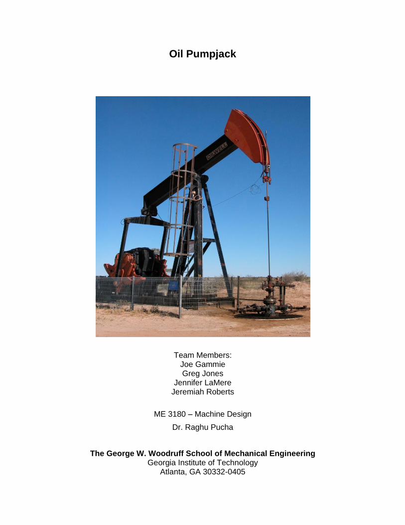
The main design goal is to limit the amount of material used in the supports to
create cheaper and lighter parts. To avoid compromising the quality of the machine by
limiting the material, every mechanical element must also maintain a factor of safety of
at least 1.5. This includes selecting a material that can support greater forces without
failing due to fracture and fatigue. It is also imperative that the structure can support
many rotations and have infinite life. Figure 1.2 shows the initial concept and
dimensions for the pumpjack. Since the goal is to limit the amount of material, the
depths are not listed since they are variable to change.
The individual design goals for each element will add more specifics in Part 3.
Figure 1.2: Pumpjack Dimensions (Metrics)
7
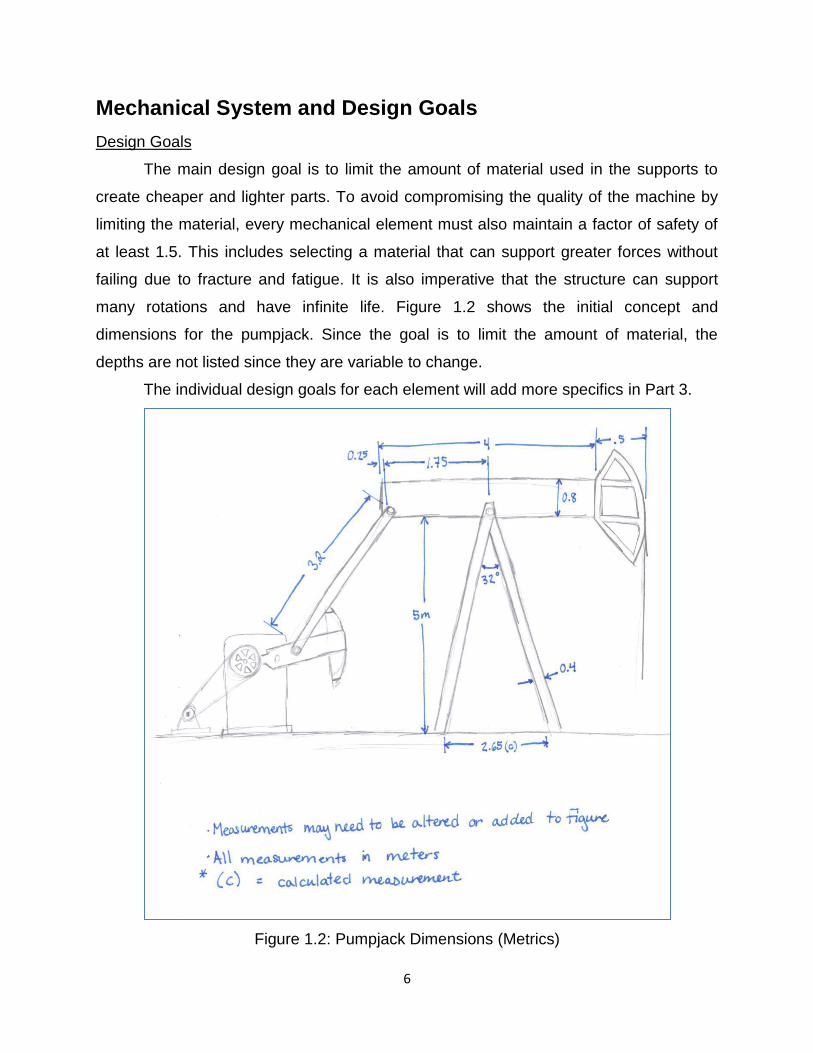
After researching the pumpjack and the mechanical elements, the system
needed to be evaluated in English units. Most of the available data is from American oil
fields, listing pressures in pound per squared inch and weights in pound-mass. Thus the
distances and measurements from Figure 3 were converted from meters to feet. Below
in Figure 1.3, the pumpjack has been redrawn to display the English dimensions and
forces.
Figure 1.3: Pumpjack Dimensions (English)
The forces displayed in the table are based on an average from Table 1.2. It lists
different types of pumpjacks, from machines used on oil fields to large off-shore oil rigs.
Table 1.2: Forces Research
Field Speed (rpm) Design Pressure Hydrotest Pressure
Holstein 5881 586 bar/8500 psi 879 bar/12750 psi
Atlantis 6200 630 bar/9140 psi 879 bar/12750 psi
Thunderhorse 5820-5997 736 bar/10675 psi 957 bar/13880 psi
Mars 5320 597 bar/8759 psi 776 bar/11255 psi

8
Management Tools
The team’s selection of the pumpjack comes after careful consideration of
several other noteworthy options. These options include a lawnmower engine, pasta
roller, and toy helicopter. Ultimately the choice of the oil pumpjack comes on the heels
of the realization that many of the other options do not have enough components for
each team member to analyze their own part. The pumpjack is ideal for this application
because of its high number of moving or active components and the wide variety of
parts that can be analyzed. For analysis the team chooses to analyze bolted joints, a
welded joint, a wire rope, shafts, and bearings.
o Joe Gammie is performing the analysis of the bolted joints.
o Jennifer LaMere is performing the analysis of the wire rope.
o Jeremiah Roberts is performing the analysis of the shafts.
o Gregory Jones is performing the analysis of the welded joint.
o And, finally, the team is performing the analysis of the bearings
collectively.
The following is a timeline of events as there are unfolding this semester and when everything will be completed by.
Table 1.3: Project Timeline
Project Proposal 9/17/2012
Introduction 9/24/2012
Mechanical Design Goals 10/19/2012
Mechanical Elements 10/29/2012
Individual Component Analysis 11/26/2012
Group Part Analysis 11/26/2012
Conclusion 11/28/2012
Final Compilation 11/30/2012

9
Part 3:
Mechanical Elements

10
Mechanical Elements
Bolted Joints – Joe Gammie
Introduction
The bolted joints in the pump jack assembly serve to connect the Samson
beams, as seen in Figure 3.1, to the baseplate or concrete below the structure. The
walking beam and horse head are mounted to the Samson support subassembly. In
essence, the bolted joints at the base of the pump jack provide the necessary
stabilization and loading for the entire structure rocking structure. In order to insure that
the pump jack will be adequately supported throughout the duration of its lifespan and
operation, it is vital to choose the correct size, material, and number of bolts for each of
the three Samson supports in the design.
Figure 3.1: Pump Jack Diagram
The design of the bolted joints involved analyzing two specific Samson arm
scenarios. The back Samson support beam will support one half of the weight of the
horsehead-beam assembly, while the two forward Samson beams will equally share the
other half of the weight. This results in a very large shear force on the bolts that must be
designed for in order to prevent failing of the joint.
Back Samson Support Beam Forward Samson
Support Beams
Base Mount
11
Assumptions and Design Goals
Certain assumptions must be made in order carry out the design analysis. These
assumptions will be used throughout the design process and will also be further
explained.
The weight of the Samson supports will be neglected when calculating loading
The bolts will mount into a thick concrete base support
The vertical weight of the machine is supported by the concrete base
Length to diameter ratio of the bolt will be 4:1
Shear stress is the limiting factor when designing the bolt assembly
Weight of Samson supports are negligible
The design will place emphasis on the diameter, material, and number of bolts in
each mount
The design goal for the forthcoming analysis is to determine optimum number bolts
and bolt diameter necessary to secure the pump jack to the concrete base with a factor
of safety of n = 1.5.
Force Analysis
In order to analyze the shear force that the bolts in each mount need to tolerate,
a force analysis must be completed. The objective is to determine the vertical loading
on the support structure shown in Figure 3.2.
12
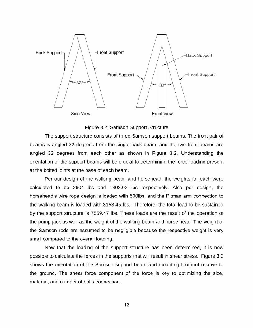
Figure 3.2: Samson Support Structure
The support structure consists of three Samson support beams. The front pair of
beams is angled 32 degrees from the single back beam, and the two front beams are
angled 32 degrees from each other as shown in Figure 3.2. Understanding the
orientation of the support beams will be crucial to determining the force-loading present
at the bolted joints at the base of each beam.
Per our design of the walking beam and horsehead, the weights for each were
calculated to be 2604 lbs and 1302.02 lbs respectively. Also per design, the
horsehead’s wire rope design is loaded with 500lbs, and the Pitman arm connection to
the walking beam is loaded with 3153.45 lbs. Therefore, the total load to be sustained
by the support structure is 7559.47 lbs. These loads are the result of the operation of
the pump jack as well as the weight of the walking beam and horse head. The weight of
the Samson rods are assumed to be negligible because the respective weight is very
small compared to the overall loading.
Now that the loading of the support structure has been determined, it is now
possible to calculate the forces in the supports that will result in shear stress. Figure 3.3
shows the orientation of the Samson support beam and mounting footprint relative to
the ground. The shear force component of the force is key to optimizing the size,
material, and number of bolts connection.
13
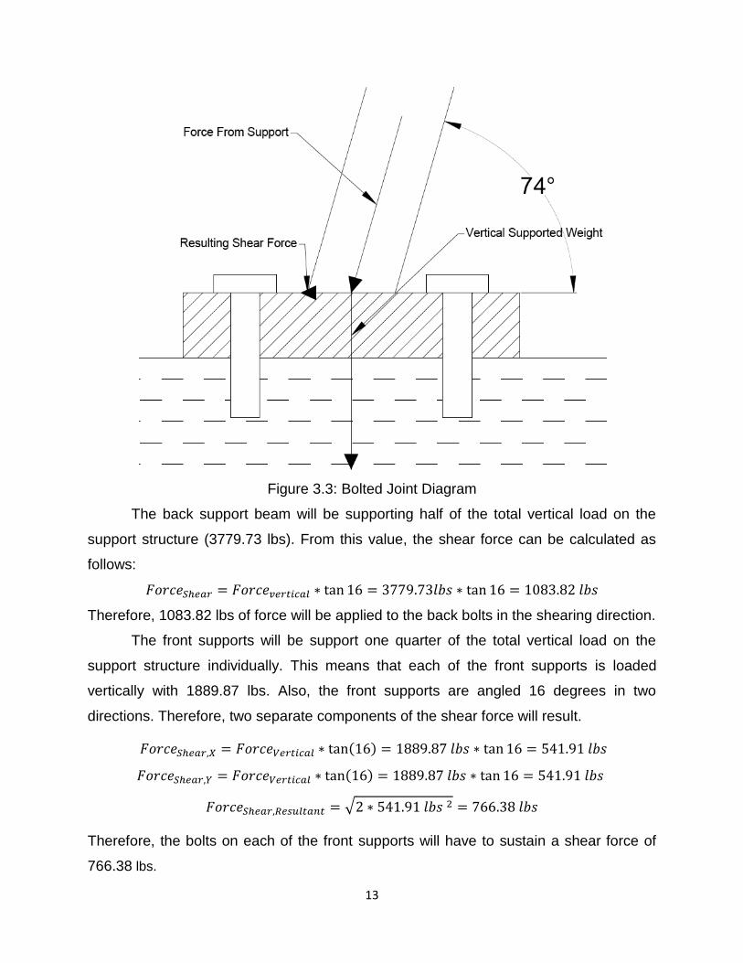
Figure 3.3: Bolted Joint Diagram
The back support beam will be supporting half of the total vertical load on the
support structure (3779.73 lbs). From this value, the shear force can be calculated as
follows:
Therefore, 1083.82 lbs of force will be applied to the back bolts in the shearing direction.
The front supports will be support one quarter of the total vertical load on the
support structure individually. This means that each of the front supports is loaded
vertically with 1889.87 lbs. Also, the front supports are angled 16 degrees in two
directions. Therefore, two separate components of the shear force will result.
( )
( )
√
Therefore, the bolts on each of the front supports will have to sustain a shear force of
766.38 lbs.
14
Welded Joints – Greg Jones
Introduction & Design Goals:
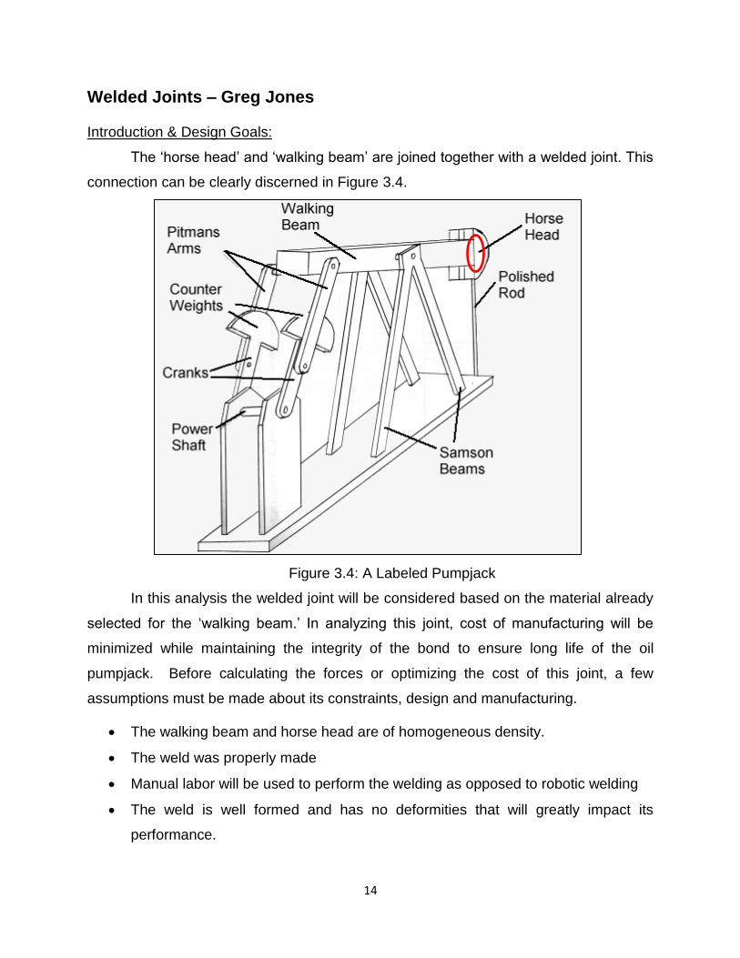
The ‘horse head’ and ‘walking beam’ are joined together with a welded joint. This
connection can be clearly discerned in Figure 3.4.
Figure 3.4: A Labeled Pumpjack
In this analysis the welded joint will be considered based on the material already
selected for the ‘walking beam.’ In analyzing this joint, cost of manufacturing will be
minimized while maintaining the integrity of the bond to ensure long life of the oil
pumpjack. Before calculating the forces or optimizing the cost of this joint, a few
assumptions must be made about its constraints, design and manufacturing.
The walking beam and horse head are of homogeneous density.
The weld was properly made
Manual labor will be used to perform the welding as opposed to robotic welding
The weld is well formed and has no deformities that will greatly impact its
performance.
15
The driving forces from the two Pitman Arms always act in the y axis and
fluctuate from +785.7 lbs to -785.7 lbs with each rotation (this information stems
from the analysis performed by Jeremiah Roberts)
The weight of the walking beam and horse head are not neglected
The force exerted by the wire rope is a constant 500 lbs.
The alternating moment and stresses that the joint experiences are less than the
static stress it experiences under maximum loading.
The weld weight is negligible compared to the overall weight of the beam.
To begin the design, the pressure and forces exerted by the underground oil had
to first be determined and the power output of the shaft driving the Pitman Arms
determined. Then, the material of the walking beam was determined in portion of the
analysis that analyzed the support beams. The same material (AISI 1080 steel) was
used for the horse head because it allows a good weld to be formed without using a
more expensive form of welding. The type, geometry, and quality of the weld are all
variable and were optimized through the following process.
Force Analysis:
Without knowing for sure which position of the pumpjack would create the most
stress on the joint, code in MATLAB (Appendix B) was written that determined the force
and moment experienced within the joint at any given angle. This proved especially
difficult for the team because, due to its oscillating motion, the forces exerted by the
Pitman Arms and the Samson Beams actually vary greatly with the angle of the walking
beam. As a result, the code calculates all these forces and moments based on the
angle of the beam. At the site of the joint, the force exerted on it is actually a constant
1.82 kips. This is true because the two variable forces are both on one side of the joint.
These variations cause the forces to cancel internally within the beam because it
undergoes no deformation, but instead simply creates a moment moves the beam
between its two extrema.
The moment was found to be a greatest at the negative extrema (an angle of -
0.6404 radians off the horizontal). This moment is -201.67 kips/inch and exerts itself
only momentarily on the beam.
16
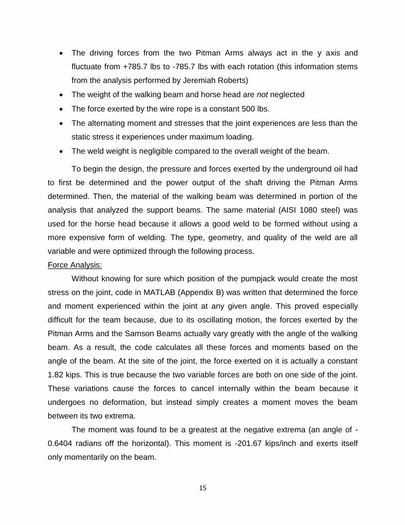
Figure 3.5: Beam Free Body Diagram
As shown in the figure above, the forces considered were the wire rope’s tension,
weight of the walking beam, weight of the horse head, force exerted by the pitman
arms, and reaction at the site of the support.
17
Wire Rope – Jennifer LaMere
Introduction & Design Goals
The wire rope needs to be able to support the force caused by the pressurized
extraction of liquid. It needs to be able to withstand unlimited rotations and thus have
unlimited life. The wire rope does not directly align with the overall design goal, since
the weight of the rope is negligible compared to the weight of the other components.
However the rope will directly transmit the input force to the attached welded joints and
thus needs to be able to support a large load.
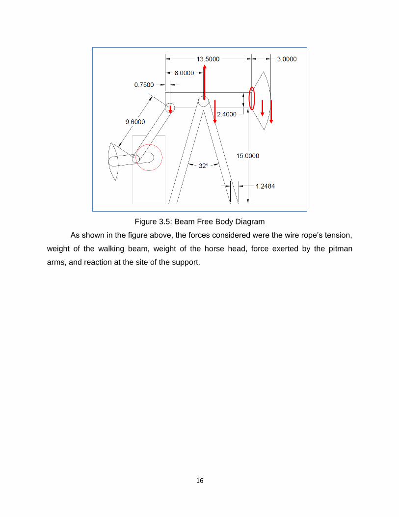
There are several parameters that limit the design of the wire rope. According to
the free body diagram in Figure 3.6, the load that it supports is substantial, at about 500
lbs. This is comparable to the weight of an elevator, which serves as a reference point
when deciding the numbers.
Figure 3.6: Free Body Diagram
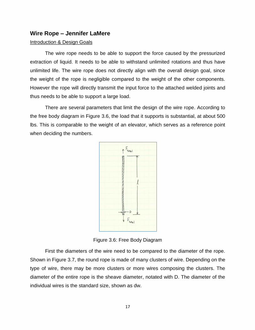
First the diameters of the wire need to be compared to the diameter of the rope.
Shown in Figure 3.7, the round rope is made of many clusters of wire. Depending on the
type of wire, there may be more clusters or more wires composing the clusters. The
diameter of the entire rope is the sheave diameter, notated with D. The diameter of the
individual wires is the standard size, shown as dw.
18
Figure 3.7: Rope Composition.
The strength of the rope is partially determined by these two geometries. The
ratios of the diameters have restrictions and limits depending on the load. For 500 lbs,
the equation below is the allowable range for the diameter ratio.
Next the equivalent bending load, notated as Fb, is the force of the static load
that the rope must be able to support. Upon looking at the free body diagram, the static
load is simply 500 lbs. The equation below displays the minimum weight.
The next parameter is the factor of safety. The machine poses no risk to human
life, since it does not transport humans and its operation is mostly automotive. Thus the
factor of safety does not have to be above 8. However, the load is large and only
supported by one rope. Thus the factor of safety is comparable to that of an elevator, as
shown in below.
The allowable maximum pressure is based on the material selected. Some of the
material options are obsolete for this usage, since wood is not flexible enough and cast
iron is not strong enough. After the diameter is chosen, Table 3.1 will be used to check
that the pressure will be within range.

19
Table 3.1: Maximum Allowable Pressure
The ration between pressure and allowable tensile strength of the wire is notated
by (p/Su). Based on Figure 3.8, the ratio dictates the number of bends that a wire can
withstand without failure. In order for the rope to have a long life, the ratio must be less
than 0.001.
Figure3.8: Pressure-Strength Ratio
For ultimate tensile strength, the value is dependent on the force and diameters.
The following equation shows how to calculate the desired value. For typical improved
plow steel, the range for ultimate tensile strength is between 240 and 280 kpsi.

20
Design & Force Analysis
To begin the design of the wire rope, Table 3.2 has been compiled to list the
knowns and the parameters that were derived from the design goals. After a diameter,
material, and structure have been selected, these are the key values that must be
satisfied in order for the combination to be considered.
Parameter Value
Load, F 500 lbs
Diameter Ratio ≤ 1000
Factor of Safety ≥ 6
Pressure * Dependent on Table
Ultimate Tensile Strength 240 ≤ Su ≤ 280
Table 3.2: Design Parameters
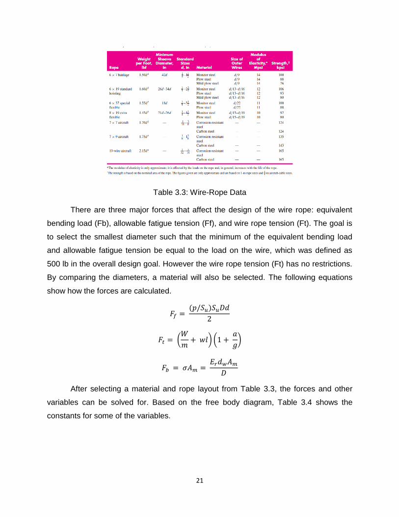
The following table lists data based on a variety of types of wire rope. The
properties of each type of rope are dependent on the wire diameter, d, and the material.
Shown in Table 3.3, the many options allow for customization of the material and size.
The range of diameters in the fourth column affects the weight per foot and the
minimum sheave diameter, as well as the size of the other wires. The Modulus of
elasticity and strength are determined by the materials. The table has also been
rearranged to easier access the data and is shown in Appendix D.
21
Table 3.3: Wire-Rope Data
There are three major forces that affect the design of the wire rope: equivalent
bending load (Fb), allowable fatigue tension (Ff), and wire rope tension (Ft). The goal is
to select the smallest diameter such that the minimum of the equivalent bending load
and allowable fatigue tension be equal to the load on the wire, which was defined as
500 lb in the overall design goal. However the wire rope tension (Ft) has no restrictions.
By comparing the diameters, a material will also be selected. The following equations
show how the forces are calculated.
( )
(
) (
)
After selecting a material and rope layout from Table 3.3, the forces and other
variables can be solved for. Based on the free body diagram, Table 3.4 shows the
constants for some of the variables.

22
Load weight W 500 lbs
Acceleration a 9.81
Gravity g 32.1
Length of Rope l 15
Number of Ropes m 1
Area of Wire Am 0.38d2
Table 3.4: Known Variables
In order to select the best option, all of the scenarios listed in Table 3.3 must be
tested. The best way to complete this is to use a recursive method. In Part 3 of the
report, the design steps are formulated into a MATLAB code to produce results for
every combination of structure, material, and diameter.

23
Shafts – Jeremiah Roberts
Introduction:
The power shaft can be arbitrarily thought of as the driving shaft of a modified 4
bar linkage device, where the power shaft is connected to the Pitman arms and the
output rod collecting oil is connected to the main shaft, with the 4th bar being the ground.
This analogy is only used to construct a visual of what the power shaft will be doing
within the pump jack system. It can be seen with certain clarity from Figure 3.9.
The design of this shaft involved constructing multiple ways the power shaft can
be linked to the pump jack body, and also how many Pitman arms will be used to
support the load.
Figure 3.9: Pumpjack schematic (note the power shaft)
In this analysis two straight shafts will be considered for Pitman’s arms; material
selection and performance optimization will be conducted for optimal power shaft
design. Before calculating forces and such on these elements, a few assumptions must
be made about the process of design. These assumptions will be more used and
explained during further design elements.

24
The power input will be constant and in the form of rotation around the reaction
through center of shaft.
The shaft will be operating at a constant speed.
The weight of the power shaft will be neglected.
The nature of design will emphasize moment analysis and not torque.
To begin the design, the pressure and forces exerted by the underground oil had
to first be determined. Then, working backwards, the pump jack body’s forces were
calculated, eventually ending on how much downward force is exerted from the main
shaft to the power shaft, which conversely tells us how much force comes from the
power shaft. This force will be used as a mean operating force required for operation of
the motor and power shaft.
A few constraints that will be referenced throughout this section in line with power
shaft design are the following:
1. [length of Pitman’s arms]
2. [vertical force required for moving pump jack]
3. ⁄ [angular velocity of crank arms]
4. [factor of safety for power shaft]
5. [total length of power shaft]
6. [diameter of power shaft, determined from Pitman’s arms and system]
This means there is a lot of flexibility in design, as material factors, material selection,
and input torque are all variable. It also means it is designed to withstand a maximum of
2.0 times the max loading conditions (785.7 lbf), which is 1571.4 lbf.
Design Goals:
The power shaft may initially seem to be in a confusing spot. It is actually the
shaft that powers the cranks that move the arms. It is convenient to note that it will be
supplying rotational motion to the crank arms which in turn moves the Pitman Arms. The
input power is supplied through a lone gear located dead center of the power shaft. A
diagram of the design in a 2D view can be seen below.

25
Figure 3.10: Power Shaft Force Analysis
The goal of this shaft is to supply rotational torque to the crank arms, which turn
the Pitman arms and allow the pump jack to rock back and forth and suction oil from
deep underground. If this arm can supply a minimum of 785.7 lbf to the cranks, then
they can translate that force to the main shaft. This means that the design goals should
be to optimize rigidity and strength of the material while decreasing material size. The
material size is already basically determined, since the arms that deliver the power are
already set. This means that the diameter of the shaft is 6 inches and the gear is
located in the middle.
The reaction forces are already known as well, since it hinges on two points.
These are the free body diagram, along with the two output forces that are both half of
785.7 lbf divided between the two outside arms, as well as the force coming from the
power input of the gear. With these five forces the deflection angles and length can all
be determined once a material is chosen, and that is where this design is focused,
material selection to fit the required forces and minimize the deflection angles and
length.
26
Force Analysis:
In order for the pump jack to maintain constant motion, its acceleration must be
zero. This means that the forces on the Pitman’s arms will be equal at the top and
bottom so that the beam is not accelerating. We then can use the max loading condition
force 785.7 lbf and split this equally between the two arms to determine what the
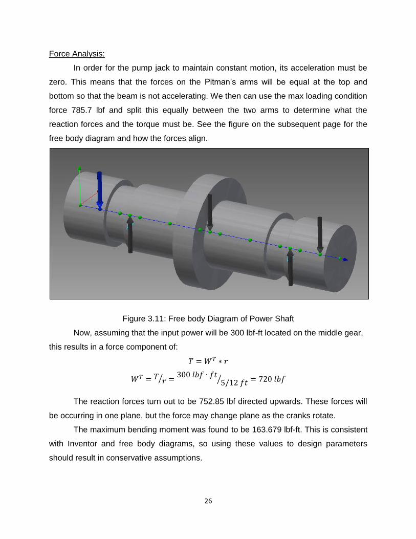
reaction forces and the torque must be. See the figure on the subsequent page for the
free body diagram and how the forces align.
Figure 3.11: Free body Diagram of Power Shaft
Now, assuming that the input power will be 300 lbf-ft located on the middle gear,
this results in a force component of:
⁄
⁄
The reaction forces turn out to be 752.85 lbf directed upwards. These forces will
be occurring in one plane, but the force may change plane as the cranks rotate.
The maximum bending moment was found to be 163.679 lbf-ft. This is consistent
with Inventor and free body diagrams, so using these values to design parameters
should result in conservative assumptions.
27
Bearing – Group Design
Introduction:
The bearing design was focused at the hinge of the support arms for the main
shaft. These are located right near the middle of the main shaft beam. From the
analysis of the reactions from the main shaft, the reaction forces on the bearing will
actually be half of the force coming from the main supports, since there are two
bearings on opposite sides supporting the main shaft.
Design Goals:
The goal for optimizing the bearings was more standardized than the other part
designs, since bearings have relatively set dimensions and the only change would be to
pick a different type or set of bearing. The design goal chosen for the main shaft
bearings was to pick the most compact and weight-supportive bearings so that there
would be a reliability of at least 0.95. The bearings components are small compared to
the rest of the machine, so the size is not as important as the reliability over its lifetime.
A few design constraints are also required. The rotation speed is determined from the
power input found from the power shaft and the moment and degree analysis from the
main shaft head done in the welded joints analysis, which works out to rotate at 11.1
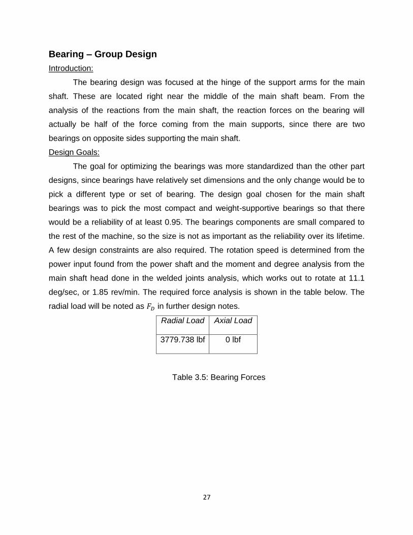
deg/sec, or 1.85 rev/min. The required force analysis is shown in the table below. The
radial load will be noted as in further design notes.
Radial Load Axial Load
3779.738 lbf 0 lbf
Table 3.5: Bearing Forces

28
Part 4:
Studies and Design Optimizations

29
Studies and Design Optimizations
Bolted Joints – Joe Gammie
Design & “What If” Analysis
After calculating the shear force for each of the three bolted joints, the correct material,
size, and number of bolts must be determined. Shear force, yield strength, number of bolts, and
shear stress are related in the following manner:
( )
( )
( )
( )
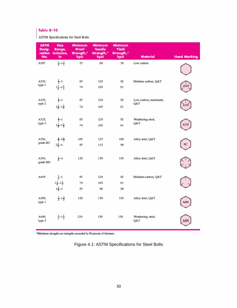
ASTM Specifications for steel bolts will be used to conduct the analysis. These
specifications can be seen in Figure 4.1.
In order to analyze all possible scenarios, bolt diameters will be chosen to vary by a
quarter inch from .25in to 4in, and the number of bolts per bolted connection will spread from 2
to 14 in increments of 2. Utilizing MATLAB, code was produced than inputted desired factor of
safety and maximum yield strength and produced each working combination of diameters and
number of bolts where the calculated yield strength was equal to or lower than desired. The
MATLAB code can be found in its entirety in Appendix A. Seeing as the goal of the design
process is to minimize material and cost, a factor of safety of 1.5 was chosen for the entire
pump jack. Therefore, a factor of safety equal to 1.5 will be chosen for the bolted joint analysis
as well. The resulting yield stress values for the front and back supports with a minimum design
yield stress of 130 kpsi and 100 kpsi respectively can be found in Tables 4.2-4.5.
30
Figure 4.1: ASTM Specifications for Steel Bolts

31
Design Case 1: n=1.5, Sy=130kpsi
FRONT SUPPORTS
Table 4.2: Front Support Results for Design Case 1
BACK SUPPORT
Table 4.3: Back Support Result for Design Case 1
Design Case 2: n=1.5, Sy = 99 kpsi
FRONT SUPPORTS
Table 4.4: Front Support Results for Design Case 2
Number of Bolts
Dia
met
er o
f B
olt
Number of Bolts
Number of Bolts
Dia
met
er o
f B
olt
D
iam
eter
of
Bo
lt
32
BACK SUPPORT
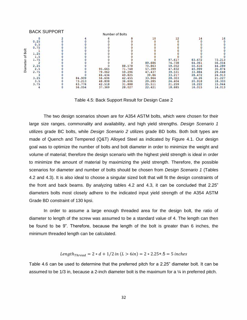
Table 4.5: Back Support Result for Design Case 2
The two design scenarios shown are for A354 ASTM bolts, which were chosen for their
large size ranges, commonality and availability, and high yield strengths. Design Scenario 1
utilizes grade BC bolts, while Design Scenario 2 utilizes grade BD bolts. Both bolt types are
made of Quench and Tempered (Q&T) Alloyed Steel as indicated by Figure 4.1. Our design
goal was to optimize the number of bolts and bolt diameter in order to minimize the weight and
volume of material; therefore the design scenario with the highest yield strength is ideal in order
to minimize the amount of material by maximizing the yield strength. Therefore, the possible
scenarios for diameter and number of bolts should be chosen from Design Scenario 1 (Tables
4.2 and 4.3). It is also ideal to choose a singular sized bolt that will fit the design constraints of
the front and back beams. By analyzing tables 4.2 and 4.3, it can be concluded that 2.25”
diameters bolts most closely adhere to the indicated input yield strength of the A354 ASTM
Grade BD constraint of 130 kpsi.
In order to assume a large enough threaded area for the design bolt, the ratio of
diameter to length of the screw was assumed to be a standard value of 4. The length can then
be found to be 9”. Therefore, because the length of the bolt is greater than 6 inches, the
minimum threaded length can be calculated.
⁄ ( ) .5
Table 4.6 can be used to determine that the preferred pitch for a 2.25” diameter bolt. It can be
assumed to be 1/3 in, because a 2-inch diameter bolt is the maximum for a ¼ in preferred pitch.
Number of Bolts
Dia
met
er o
f B
olt

33
Table 4.6: Preferred Pitches for ASME Threads
Final Design Summary
Design of Front Bolted Joint
n = 1.5 Max Yield Strength = 130 kpsi
Shear Loading 766.38 lbs
Diameter of Bolt 2.25”
Number of Bolts 4
Design of Back Bolted Joint
n = 1.5 Max Yield Strength = 130 kpsi
Shear Loading 1083.82 lbs
Diameter of Bolt 2.25”
Number of Bolts 6
Total Number of Bolts 12
Bolt Properties
ASTM Designation Number A354, Grade BD
Material Alloy Steel, Q&T
Head Shape Hexagonal
Length of Bolt 9”
Minimum Thread Length 5”
Pitch ⁄ Thread ASME
Verification
The verification of the design is very simple. Using the design values, the actual factor of safety
for each support can be calculated.
( )
( )
Front Bolted Joints
( )
( )
⁄
( )
⁄

34
Back Bolted Joints
( )
( )
⁄
( )
⁄
Given that the design parameter was to have a minimum factor of safety of 1.5, both
these bolted joints meet the constraints and, therefore, the design is verified.
Discussion
The bolted connection design encompassed analyzing the shear forces from the loading
of the pump jack support beams. Because the concrete support slab provides the entirety of the
vertical support of the pump jack assembly, the bolted joint loading is essentially only in shear
strain. The shear strain was calculated based on the compression forces in the Samson support
from supporting the weight and loading on the walking beam and horse head. These values
were both found to be greater than 700 pounds, representing a very large and significant shear
force on the bolted connections. Therefore, the design of these joints is anything but trivial.
By assessing that diameter of the bolts and the number of the bolts are both values that
can be varied; the design problem becomes one that can be optimized by striking a balance
between the two. The system was optimized to limit excess material and strength over a factor
of safety of 1.5. This results in limiting the cost of the design as well as the weight.
“What If” analysis allowed for a conclusion of 4 bolts of 2.25” diameter for the two front
supports and 6 bolts of 2.25” diameter for the back support. Utilizing high strength A354 grade
BD steel allowed for the number and sizes of the bolts to be limited the most. The decision to
use the same material and size bolt for each connection and merely vary the number of bolts
used at each connection allows the design to be flexible in maintenance, part supply, and
interchangeable. Overall, the design met its factor of safety restraint of 1.5 and will fully support
the pump jack through its operation.
35
Welded Joints – Greg Jones
Design:
The actual design goal is to minimize the cost associated with forming this joint,
while still ensuring its integrity. This design goal was decided upon because optimizing
the weight of this weld would do little to help lighten the overall weight of the beam, in
fact, one of the team’s assumptions is that the weld weight is negligible compared to the
weight of the beam.
The cost of welding a joint that is welded by hand is dependent mostly upon the
labor costs because of the high amount of skill required to complete a solid weld. The
team assumed that the weld would be manual because the low production rates
associated with pumpjacks would not allow payback on the sizable investment in robotic
welding equipment. To minimize labor costs, the goal is to minimize the amount of
welding that has to occur. So to review, the design goal for the welded joint is to
minimize the length of time it takes to complete the weld by minimizing the weld area.
The shape of the beam was already determined to be a rectangle with
dimensions 2.4 ft by 1 ft. A butt joint and weld will be used to join the walking beam to
the horse head because no other geometry could be determined that didn’t include
other welds or geometries that would be difficult to weld and would take longer. As a
result, code in MATLAB (Appendix B and C) was written that analyzed the geometries
shown in Figure 4.2 below from Table 9-2, which describes properties of bending welds.

36
Figure 4.2: Different Weld Geometries
These calculations were performed with 12 different weld thicknesses (shown above as h). The resulting table below corresponds to weld areas, in square inches, which the team hopes to minimize.
Weld Thickness
(h) in Inches
Parallel Vertical Welds
Parallel Horizontal
Welds
Welded on Three Sides
w/ Side Open
Welded on Three Sides w/ Bottom
Open
Full Box Weld
1 40.72 16.97 37.33 49.21 57.69
7/8 35.63 14.85 32.66 43.06 50.48
3/4 30.54 12.73 27.99 36.91 43.27
5/8 25.45 10.61 23.33 30.75 36.06
1/2 20.36 8.48 18.66 24.60 28.85
7/16 17.82 7.42 16.33 21.53 25.24
3/8 15.27 6.36 13.99 18.45 21.63
5/16 12.73 5.30 11.67 15.37 18.02
1/4 10.18 4.24 9.33 12.30 14.42
3/16 7.64 3.18 6.99 9.23 10.81
1/8 5.09 2.12 4.67 6.15 7.21
1/16 2.55 1.06 2.33 3.08 3.61
Table 4.7: Weld Areas
37
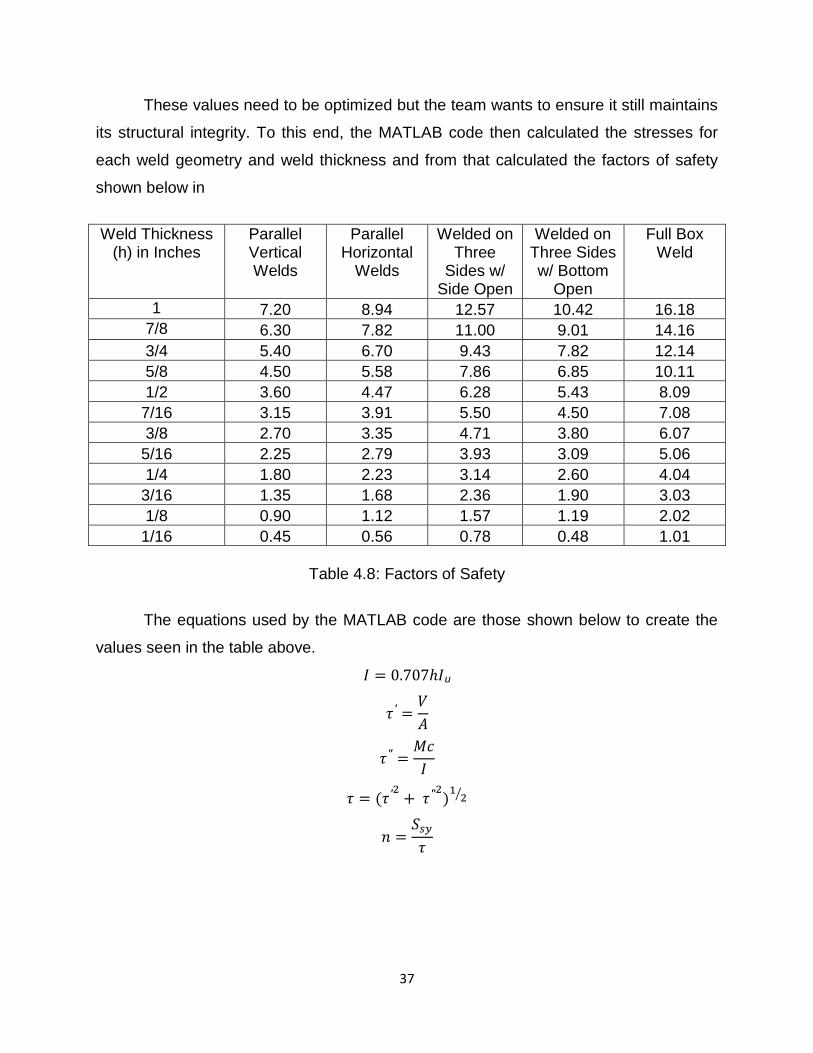
These values need to be optimized but the team wants to ensure it still maintains
its structural integrity. To this end, the MATLAB code then calculated the stresses for
each weld geometry and weld thickness and from that calculated the factors of safety
shown below in
Weld Thickness (h) in Inches
Parallel Vertical Welds
Parallel Horizontal
Welds
Welded on Three
Sides w/ Side Open
Welded on Three Sides w/ Bottom
Open
Full Box Weld
1 7.20 8.94 12.57 10.42 16.18
7/8 6.30 7.82 11.00 9.01 14.16
3/4 5.40 6.70 9.43 7.82 12.14
5/8 4.50 5.58 7.86 6.85 10.11
1/2 3.60 4.47 6.28 5.43 8.09
7/16 3.15 3.91 5.50 4.50 7.08
3/8 2.70 3.35 4.71 3.80 6.07
5/16 2.25 2.79 3.93 3.09 5.06
1/4 1.80 2.23 3.14 2.60 4.04
3/16 1.35 1.68 2.36 1.90 3.03
1/8 0.90 1.12 1.57 1.19 2.02
1/16 0.45 0.56 0.78 0.48 1.01
Table 4.8: Factors of Safety
The equations used by the MATLAB code are those shown below to create the
values seen in the table above.
u
( ) ⁄
38
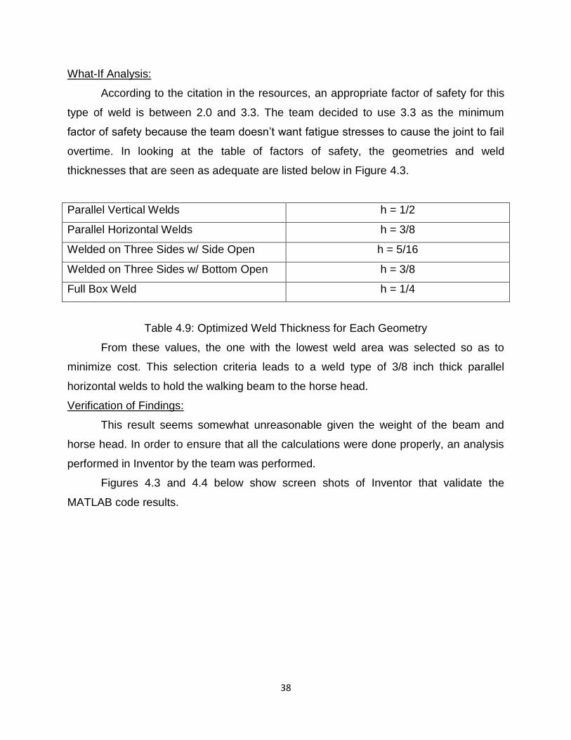
What-If Analysis:
According to the citation in the resources, an appropriate factor of safety for this
type of weld is between 2.0 and 3.3. The team decided to use 3.3 as the minimum
factor of safety because the team doesn’t want fatigue stresses to cause the joint to fail
overtime. In looking at the table of factors of safety, the geometries and weld
thicknesses that are seen as adequate are listed below in Figure 4.3.
Parallel Vertical Welds h = 1/2
Parallel Horizontal Welds h = 3/8
Welded on Three Sides w/ Side Open h = 5/16
Welded on Three Sides w/ Bottom Open h = 3/8
Full Box Weld h = 1/4
Table 4.9: Optimized Weld Thickness for Each Geometry
From these values, the one with the lowest weld area was selected so as to
minimize cost. This selection criteria leads to a weld type of 3/8 inch thick parallel
horizontal welds to hold the walking beam to the horse head.
Verification of Findings:
This result seems somewhat unreasonable given the weight of the beam and
horse head. In order to ensure that all the calculations were done properly, an analysis
performed in Inventor by the team was performed.
Figures 4.3 and 4.4 below show screen shots of Inventor that validate the
MATLAB code results.
39
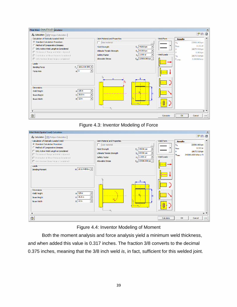
Figure 4.3: Inventor Modeling of Force
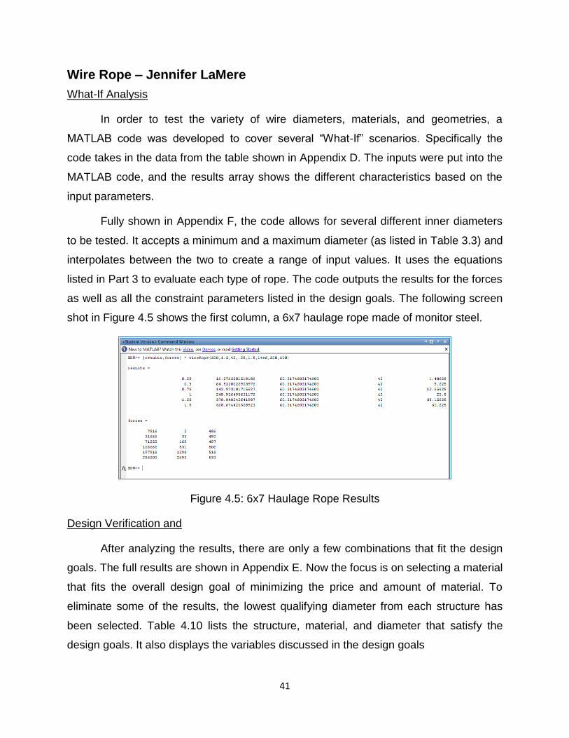
Figure 4.4: Inventor Modeling of Moment
Both the moment analysis and force analysis yield a minimum weld thickness,
and when added this value is 0.317 inches. The fraction 3/8 converts to the decimal
0.375 inches, meaning that the 3/8 inch weld is, in fact, sufficient for this welded joint.

40
Discussion:
The design of this welded joint was a rewarding process because it involved a lot
of self-teaching and when the answer was right, it all paid off. I had the opportunity to
utilize the majority of concepts introduced in chapter 9 of the book as well as price
optimization through the research of welding processes. Without the use of all the
charts, tables, and information within the text, this analysis could not have been
completed. Since this welded joint will see fluctuating stress due to a changing moment,
it is important that the weld be strong enough. In a non-idealized environment, there are
many other factors that impact the weld’s strength. For instance, the skill of the welder
is an incredibly important factor that could not be accounted for in this analysis aside
from the assumption that the weld contained no notable deformities. Aside from human
factors, welds are an incredibly strong and cost effective way of joining two pieces of
metal and it was very rewarding to design and see this joint implemented in Inventor.
41
Wire Rope – Jennifer LaMere
What-If Analysis
In order to test the variety of wire diameters, materials, and geometries, a
MATLAB code was developed to cover several “What-If” scenarios. Specifically the
code takes in the data from the table shown in Appendix D. The inputs were put into the
MATLAB code, and the results array shows the different characteristics based on the
input parameters.
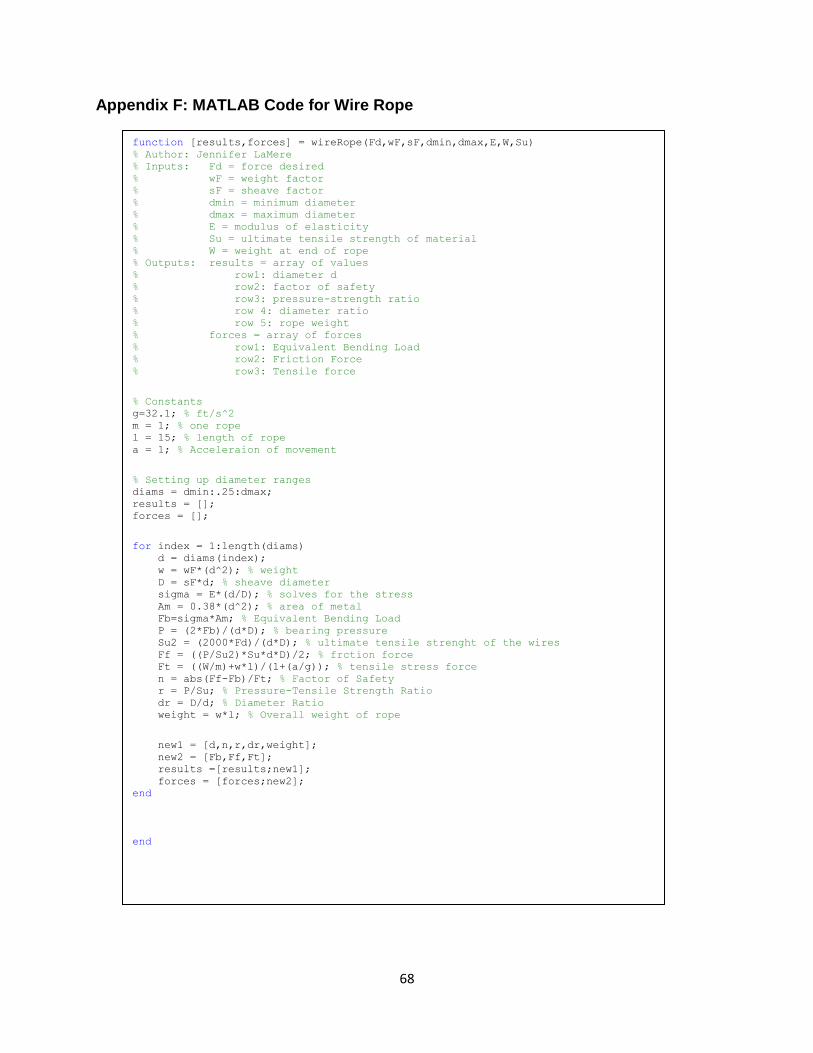
Fully shown in Appendix F, the code allows for several different inner diameters
to be tested. It accepts a minimum and a maximum diameter (as listed in Table 3.3) and
interpolates between the two to create a range of input values. It uses the equations
listed in Part 3 to evaluate each type of rope. The code outputs the results for the forces
as well as all the constraint parameters listed in the design goals. The following screen
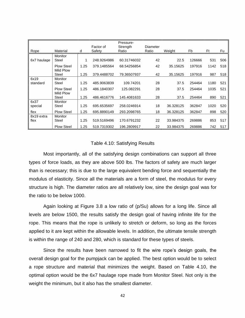
shot in Figure 4.5 shows the first column, a 6x7 haulage rope made of monitor steel.
Figure 4.5: 6x7 Haulage Rope Results
Design Verification and
After analyzing the results, there are only a few combinations that fit the design
goals. The full results are shown in Appendix E. Now the focus is on selecting a material
that fits the overall design goal of minimizing the price and amount of material. To
eliminate some of the results, the lowest qualifying diameter from each structure has
been selected. Table 4.10 lists the structure, material, and diameter that satisfy the
design goals. It also displays the variables discussed in the design goals
42
Rope Material d Factor of Safety
Pressure-Strength Ratio
Diameter Ratio Weight Fb Ft Fu
6x7 haulage Monitor Steel 1 248.9264986 60.31746032 42 22.5 126666 531 506
Plow Steel 1.25 379.1485564 68.54256854 42 35.15625 197916 1142 518
Mild Plow Steel 1.25 379.4488702 79.36507937 42 35.15625 197916 987 518
6x19 standard
Monitor Steel 1.25 485.9063839 109.74201 28 37.5 254464 1180 521
Plow Steel 1.25 486.1840307 125.082291 28 37.5 254464 1035 521
Mild Plow Steel 1.25 486.4616776 145.4081633 28 37.5 254464 890 521
6x37 special
Monitor Steel 1.25 695.6535697 258.0246914 18 36.328125 362847 1020 520
flex Plow Steel 1.25 695.8890149 293.2098765 18 36.328125 362847 898 520
8x19 extra flex
Monitor Steel 1.25 519.5169496 170.6791232 22 33.984375 269886 853 517
Plow Steel 1.25 519.7319302 196.2809917 22 33.984375 269886 742 517
Table 4.10: Satisfying Results
Most importantly, all of the satisfying design combinations can support all three
types of force loads, as they are above 500 lbs. The factors of safety are much larger
than is necessary; this is due to the large equivalent bending force and sequentially the
modulus of elasticity. Since all the materials are a form of steel, the modulus for every
structure is high. The diameter ratios are all relatively low, sine the design goal was for
the ratio to be below 1000.
Again looking at Figure 3.8 a low ratio of (p/Su) allows for a long life. Since all
levels are below 1500, the results satisfy the design goal of having infinite life for the
rope. This means that the rope is unlikely to stretch or deform, so long as the forces
applied to it are kept within the allowable levels. In addition, the ultimate tensile strength
is within the range of 240 and 280, which is standard for these types of steels.
Since the results have been narrowed to fit the wire rope’s design goals, the
overall design goal for the pumpjack can be applied. The best option would be to select
a rope structure and material that minimizes the weight. Based on Table 4.10, the
optimal option would be the 6x7 haulage rope made from Monitor Steel. Not only is the
weight the minimum, but it also has the smallest diameter.

43
Discussion
The process of selected a rope is deceivingly complex. The structure is defined
by the layout and number of several wires and the material is dependent on the inner
material as well. The diameter was the main parameter for the What-If Analysis, since
the sheave diameter, forces, factors of safety, and weight are all dependent on it. Also
wire ropes necessitate large factors of safety, since the amount of load that they
individually support is so large. The failure of such a component could cause damage to
the other structural elements as well as present a threat to human life.
After completing the Force Analysis and What-If Scenarios, there is no way to
verify the design since it is not an element available in Inventor Studio. However the
results are comparable with the constraints given in the textbook examples and text.
44
Shafts – Jeremiah Roberts
Design
To review, the design goal for the pump jack is to minimize materials so the
machine will be lighter, while maintaining or even improving strength. This means that
stress factors and material factors will be incredibly important in determining which
material type to use. Ashby charts and Tensile Strength charts will be crucial for
comparing materials together.
To begin, an explanation of where these calculations were derived. Most of the
stress calculations were done in Inventor and Excel, and an Excel sheet was
constructed to measure values without repeatedly computing calculations. The Inventor
drawings can be found throughout the text. The main values that will change are the
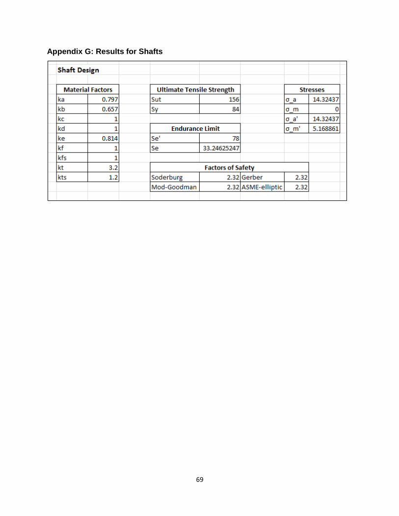
material and stress factors and the ultimate tensile strength. This Excel code can be
found in Appendix G.
To begin, stress concentration factors should be determined. With the help of
table A-21 from the ME 3180 text, the heat-treated steel AISI 1050 CD was selected for
its size vs. strength characteristics. It has ultimate tensile strength of 100 kpsi and yield
strength of 84 kpsi. Review of the Ashby chart helps determine this decision, which can
be seen in the next two figures below.

45
Figure 4.6: Ashby Chart GPa vs. Density
Figure 4.7: Ashby Chart Strength vs. Density
46
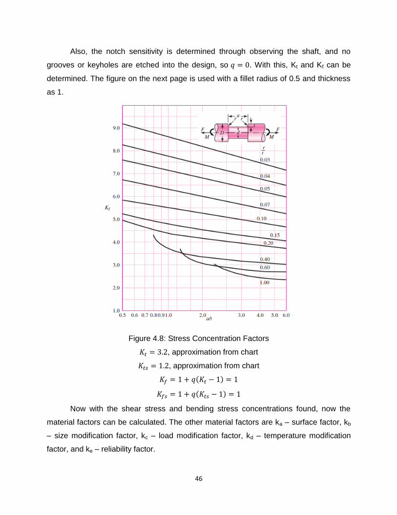
Also, the notch sensitivity is determined through observing the shaft, and no
grooves or keyholes are etched into the design, so . With this, Kt and Kf can be
determined. The figure on the next page is used with a fillet radius of 0.5 and thickness
as 1.
Figure 4.8: Stress Concentration Factors
, approximation from chart
, approximation from chart
( )
( )
Now with the shear stress and bending stress concentrations found, now the
material factors can be calculated. The other material factors are ka – surface factor, kb
– size modification factor, kc – load modification factor, kd – temperature modification
factor, and ke – reliability factor.
47
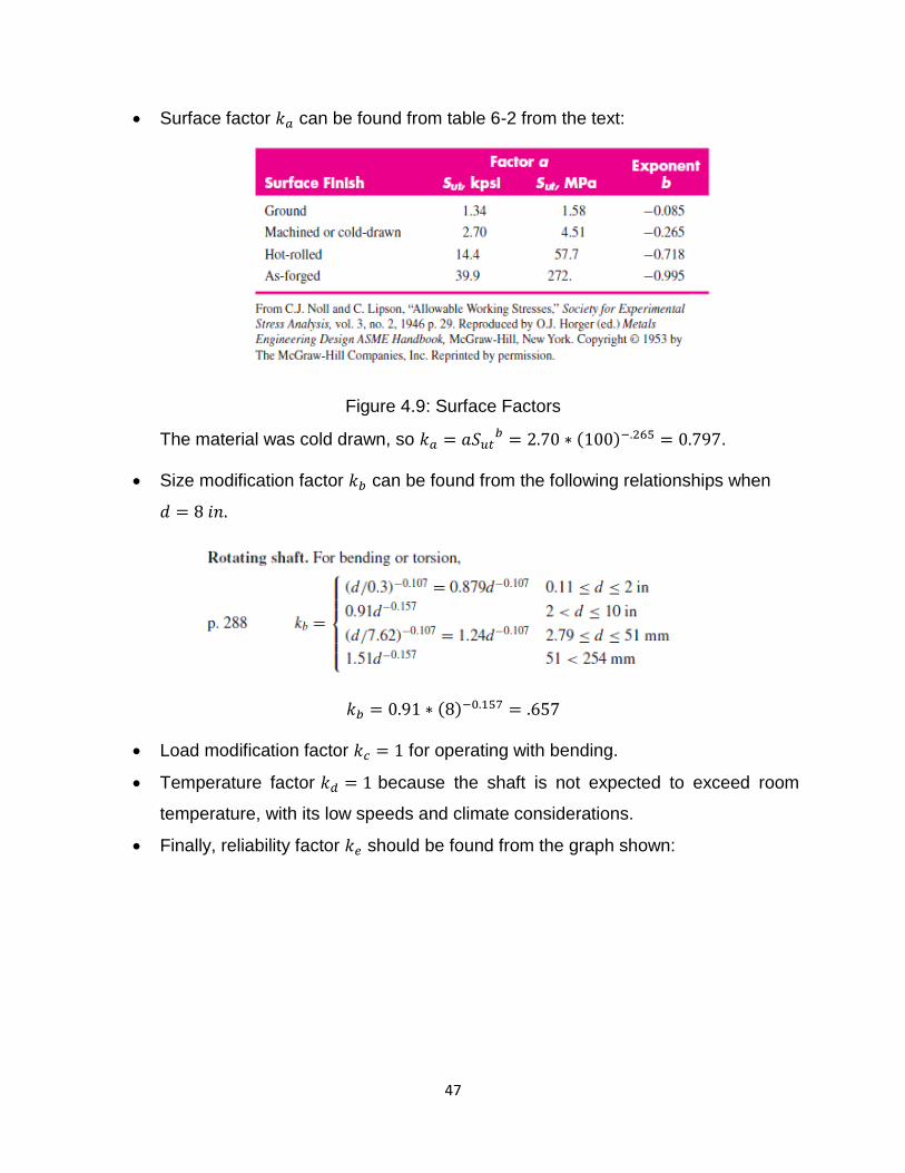
Surface factor can be found from table 6-2 from the text:
Figure 4.9: Surface Factors
The material was cold drawn, so ( ) .
Size modification factor can be found from the following relationships when
( )
Load modification factor for operating with bending.
Temperature factor because the shaft is not expected to exceed room
temperature, with its low speeds and climate considerations.
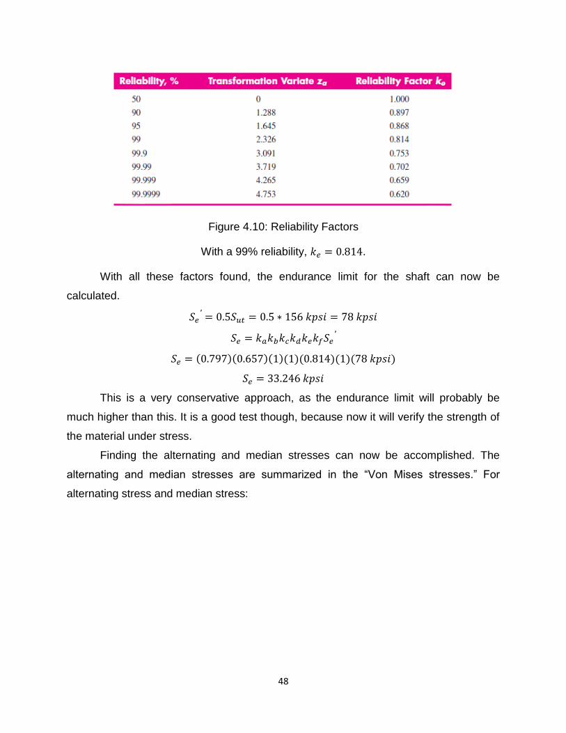
Finally, reliability factor should be found from the graph shown:
48
Figure 4.10: Reliability Factors
With a 99% reliability, .
With all these factors found, the endurance limit for the shaft can now be
calculated.
( )( )( )( )( )( )( )
This is a very conservative approach, as the endurance limit will probably be
much higher than this. It is a good test though, because now it will verify the strength of
the material under stress.
Finding the alternating and median stresses can now be accomplished. The
alternating and median stresses are summarized in the “Von Mises stresses.” For
alternating stress and median stress:

49
√
√(
)
(
)
√
√(
)
(
)
This leads to the following inputs:
√(
)
(
)
√(
)
(
)
With the Von Mises stresses the factors of safety can now be calculated, all four
different methods. Each method needs to be verified that it is above the 2.0 limit. If
every method yields a value higher than this, it can be assumed that this material
completely satisfies the restraints for the problem and could possibly even be reduced
in strength if the design goal were to reduce costs.
Soderburg:
⁄
⁄ ⁄
( )
(
)
Mod-Goodman:
⁄
⁄ ⁄
( )
(
)
Gerber:
⁄ (
⁄ )

50
( )
(
)
ASME-elliptic:
( ⁄ )
(
⁄ )
⁄
( )
(
)
And, perhaps unsurprisingly, all the safety factors work out to be the same. This
is due to the midpoint stress equaling zero. Having these factors of safety validate the
design and design choices made for the material factors.
What-If Analysis in Design
While calculating various values for the stresses, it seemed like the material
factors played a big role in determining the outcome of the safety factors. The best
what-if analysis for this design is if the material factors were different, what would the
material selection be? First the work must be done backwards. The minimum factor of
safety is 2.0, so working backwards from this allows the endurance limit to be as low as
28.648 kpsi. When reviewing the factors, the one with the most variability due to
material selection is the surface factor, ka. If all others are kept constant and this new
endurance limit is used, ka can now be as low as 0.689. This allows a host of other
materials. The following is a table of the required ultimate tensile strengths for various
types of crafted steel when ka is 0.689.
Surface Finish Respective Equation Requirement
Ground 2504.113 kpsi
Machined or cold-drawn 173.094 kpsi
Hot-rolled 68.967 kpsi
As-forged 59.103 kpsi
Table 4.11: Tensile Strength What-If Surface Factor Analysis
This is a very interesting analysis. This shows that the material selection, if it
were hot-rolled, could have a tensile strength as low as 68.967 kpsi. In fact, if it goes
higher than that it actually will fail. These values all contain a “greater than” or “less

51
than” tag with them, so that only values in that range work for the given conditions. The
only steel grades that meet these requirements are AISI 1030 annealed at 870 C for
hot-rolled, but its statistics for other things such as yield strength are so low that it is
arguably thrown out.
Looking back at this analysis also gives the idea that the safety factor could be
reduced. If the material selection is known, say AISI 1050 CD steel, then the factor of
safety could be as low as 1.5 and still be safe and not fail. This is a less conservative
approach than before, but it is still appropriate because the safety factor will be
considered with known material strengths. If everything is again calculated backwards
with this minimum safety factor, then the different tensile strength requirements are as
follows:
Surface Finish Respective Equation Requirement
Ground 87.710 kpsi
Machined or cold-drawn 101.144 kpsi
Hot-rolled 444.259 kpsi
As-forged 606.269 kpsi
Table 4.12: Tensile Strength What-If Factor of Safety Analysis
Looking at these tensile strengths, it is clear to see which ones are most
reasonable. If the factor of safety were to be 1.5, then machined or cold-drawn is the
likely best suited for the design. Hot-rolled and as-forged steel have ultimate tensile
strengths likely too high to be realistically considered for the design.
This concludes that AISI 1050 Cold Drawn steel is optimized for this design
situation, perfect specifically for its strength capacity and size reduction. It will also work
if the factor of safety considered was to be 1.5 instead of 2.0, and it will be the best
candidate for the design in cases with a variable material surface factor.
52
Discussion
The design of this shaft was a very rewarding process, mainly because it utilized
so much of the material factors and endurance limit analysis. Without utilizing all the
charts and tables all of this work would not have been completed. It is interesting to
think about this shaft in its completed spot within the design; this shaft will be turning at
a rather slow and constant rate. Since it is being subject to a constant and repeated
load, some interesting things will happen. First, it will slightly increase the time for which
it will yield. This is the case because the local member stress is lower than if it were
quickly alternating, and also because of intersecting “lines of dislocation.” This term is
used more in the mechanics of materials courses, but it can account for why metallurgy
has become popular and useful over the years and why beating a metal makes it
stronger (for a time). All of this goes into a very interesting and viable solution to the
design problem asked by this team, and the design of this shaft provides a cornerstone
for the rest of the design to operate on.

53
Bearing – Group Design
Design:
To find the bearing needed to fit the design problem, a catalog value should be
obtained and retrieved from Table 4.15, which can be found in the text and later on in
this section. The first step to finding the catalog value ( ) is to find the dimensionless
multiple of rating life, .
⁄
Where is desired life and is rated life. Desired life is given by the formula
seen below, where is the life in kilohours (kh) and n is the speed in rev/min.
Rated life is typically set to 106 hours and is the commonly accepted value in
many design problems as well as the text. The life in kilohours will be set to 175 kh; this
can be seen by referencing Table 13.
Table 4.13: Desired life depending on machine factors
With these values, the parameter is found to be 19.425. The next term to find
is , the reliability factor. The equation is shown below:
{ (
)
}
54
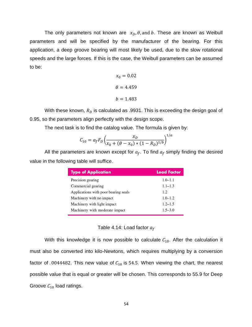
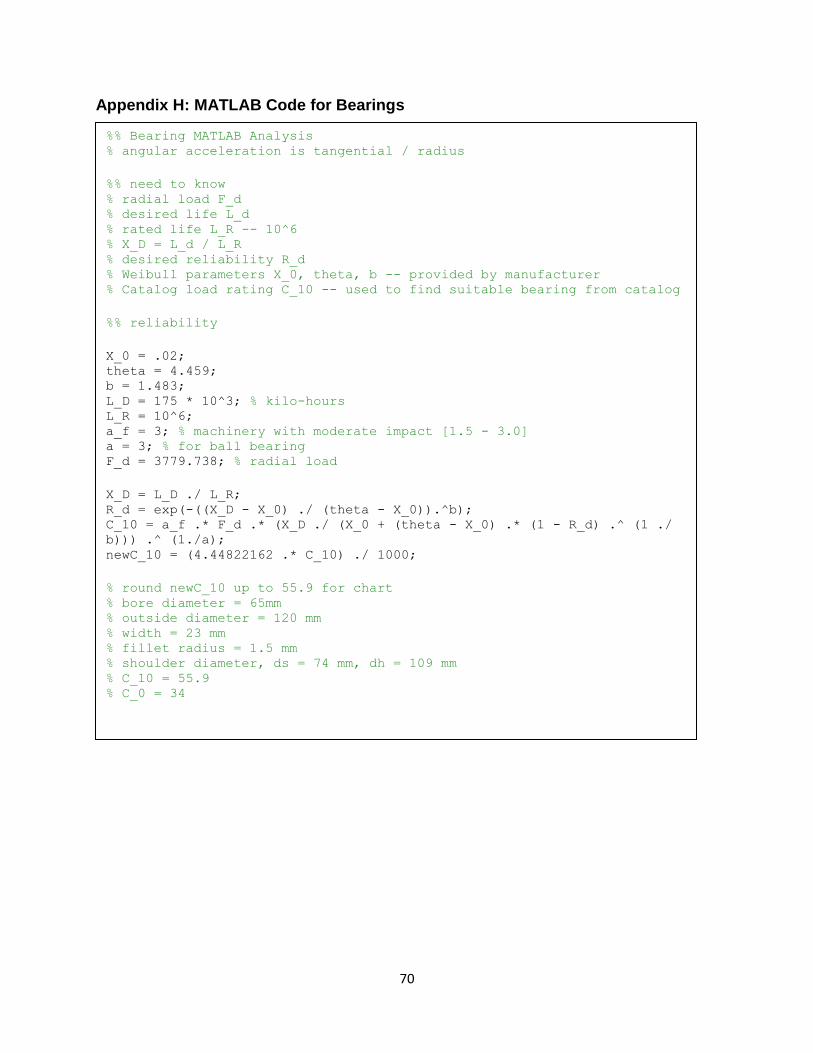
The only parameters not known are . These are known as Weibull
parameters and will be specified by the manufacturer of the bearing. For this
application, a deep groove bearing will most likely be used, due to the slow rotational
speeds and the large forces. If this is the case, the Weibull parameters can be assumed
to be:
With these known, is calculated as .9931. This is exceeding the design goal of
0.95, so the parameters align perfectly with the design scope.
The next task is to find the catalog value. The formula is given by:
(
( ) ( ) )
All the parameters are known except for . To find simply finding the desired
value in the following table will suffice.
Table 4.14: Load factor
With this knowledge it is now possible to calculate . After the calculation it
must also be converted into kilo-Newtons, which requires multiplying by a conversion
factor of . This new value of is . When viewing the chart, the nearest
possible value that is equal or greater will be chosen. This corresponds to 55.9 for Deep
Groove load ratings.

55
Table 4.15: Bearing dimensions for given values
This corresponds to the following bearing design features:
The final design issue is that of lubrication. The following chart can be used to
determine between the use of oil or grease.
56
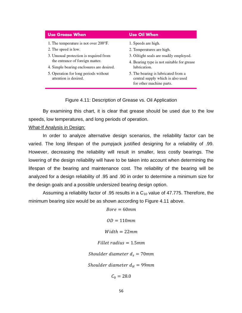
Figure 4.11: Description of Grease vs. Oil Application
By examining this chart, it is clear that grease should be used due to the low
speeds, low temperatures, and long periods of operation.
What-If Analysis in Design:
In order to analyze alternative design scenarios, the reliability factor can be
varied. The long lifespan of the pumpjack justified designing for a reliability of .99.
However, decreasing the reliability will result in smaller, less costly bearings. The
lowering of the design reliability will have to be taken into account when determining the
lifespan of the bearing and maintenance cost. The reliability of the bearing will be
analyzed for a design reliability of .95 and .90 in order to determine a minimum size for
the design goals and a possible undersized bearing design option.
Assuming a reliability factor of .95 results in a C10 value of 47.775. Therefore, the
minimum bearing size would be as shown according to Figure 4.11 above.
57
If a reliability factor of .90 is chosen, then the resulting C10 value is calculated to
be 45.7. The value of 43.6 from Table 4.15 will be used to assume a worst-case
scenario. The resulting bearing dimensions are as follows:
The smaller bearing designs are cheaper and consist of less material. However,
they are less robust to the heavy loading, and thus less reliable. If high reliability and
robust design were not the primary design considerations, then adopting a smaller,
leaner option would be more appropriate.
Discussion:
The large loading supported by the pump jack design mandates that the bearing
design be carefully planned and executed. The design goal to use the most compact
and weight-supportive bearings with a reliability of at least 0.95 required that the bearing
would be engineered with a calculated overhead. In the end, the constant motion and
large loading led to the acceptance of a bearing with reliability close to .99. This high
reliability is very important because of the constant motion the pump jack is expected to
undergo during operation. The resulting large, 12 cm diameter is of no surprise, as each
of the bearings must support over 3000 lbs of force. This design will insure that the
bearings will not fail during operation and loading. It is also important to note that the
design can be expected to last throughout the life cycle of the pump jack, but alternative
designs with lower reliability might be beneficial if maintenance and replacement costs
are expected and menial.
58
Part 5:
Design Goals and Conclusion

59
Design Goals and Conclusion
Upon completing the analysis and verification for the mechanical elements, the
final results can be compiled. The design goals for each element must be compiled to
ensure that they align with the overall goal and with each other.
First the factors of safety for each mechanical element are shown in Table ***.
The original design goal is for every component to have a factor of safety of at least 1.5.
Based on the designs chosen by each group member, all of the elements satisfy this
goal. The next design goal was to limit the amount of material, and thus weight, of each
element. Each group member directly addressed this when selecting the structure and
material.
Bolted Joint 1.5
Welded Joint 2.0
Wire Rope 22
Shafts 2.0
Bearings 1.6
Table 5.1: Final Factors of Safety
Overall the pumpjack was an ideal machine to design. The large number of
components allowed the group to be flexible when choosing what to model. Because
the pumpjack is used in many scenarios to pump oil, water, and other liquids, the group
could freely choose the loaded weight and amount of input power through the motor.
The individual elements, while needing different equations, had design processes that
followed the same structure. Thus each group member was able to apply skills learned
in the Machine Design course even if the material was not covered. Using these learned
methods, the final design successfully satisfied the overall and individual design goals.

60
Part 6:
Appendix
61
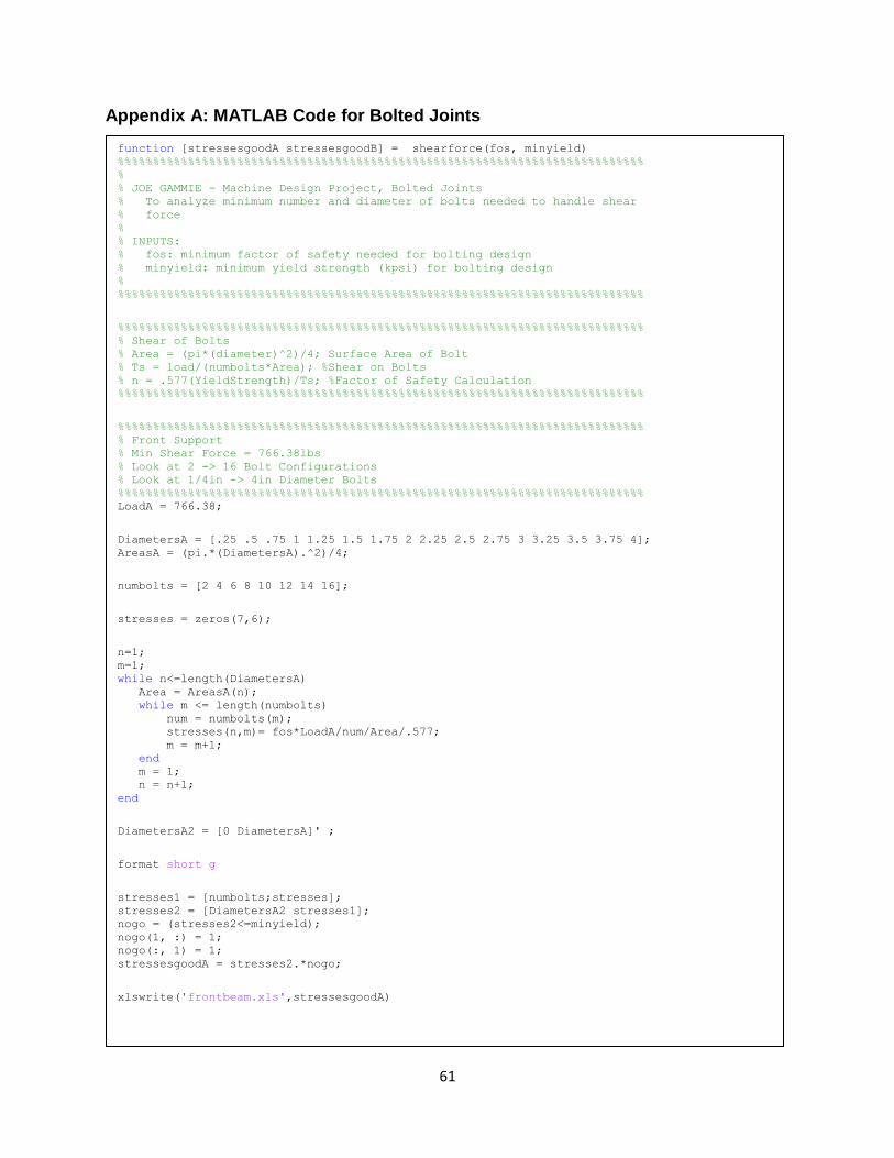
Appendix A: MATLAB Code for Bolted Joints
function [stressesgoodA stressesgoodB] = shearforce(fos, minyield) %%%%%%%%%%%%%%%%%%%%%%%%%%%%%%%%%%%%%%%%%%%%%%%%%%%%%%%%%%%%%%%%%%%%%%%%%%% % % JOE GAMMIE - Machine Design Project, Bolted Joints % To analyze minimum number and diameter of bolts needed to handle shear % force % % INPUTS: % fos: minimum factor of safety needed for bolting design % minyield: minimum yield strength (kpsi) for bolting design % %%%%%%%%%%%%%%%%%%%%%%%%%%%%%%%%%%%%%%%%%%%%%%%%%%%%%%%%%%%%%%%%%%%%%%%%%%%
%%%%%%%%%%%%%%%%%%%%%%%%%%%%%%%%%%%%%%%%%%%%%%%%%%%%%%%%%%%%%%%%%%%%%%%%%%% % Shear of Bolts % Area = (pi*(diameter)^2)/4; Surface Area of Bolt % Ts = load/(numbolts*Area); %Shear on Bolts % n = .577(YieldStrength)/Ts; %Factor of Safety Calculation %%%%%%%%%%%%%%%%%%%%%%%%%%%%%%%%%%%%%%%%%%%%%%%%%%%%%%%%%%%%%%%%%%%%%%%%%%%
%%%%%%%%%%%%%%%%%%%%%%%%%%%%%%%%%%%%%%%%%%%%%%%%%%%%%%%%%%%%%%%%%%%%%%%%%%% % Front Support % Min Shear Force = 766.38lbs % Look at 2 -> 16 Bolt Configurations % Look at 1/4in -> 4in Diameter Bolts %%%%%%%%%%%%%%%%%%%%%%%%%%%%%%%%%%%%%%%%%%%%%%%%%%%%%%%%%%%%%%%%%%%%%%%%%%% LoadA = 766.38;
DiametersA = [.25 .5 .75 1 1.25 1.5 1.75 2 2.25 2.5 2.75 3 3.25 3.5 3.75 4]; AreasA = (pi.*(DiametersA).^2)/4;
numbolts = [2 4 6 8 10 12 14 16];
stresses = zeros(7,6);
n=1; m=1; while n<=length(DiametersA) Area = AreasA(n); while m <= length(numbolts) num = numbolts(m); stresses(n,m)= fos*LoadA/num/Area/.577; m = m+1; end m = 1; n = n+1; end
DiametersA2 = [0 DiametersA]' ;
format short g
stresses1 = [numbolts;stresses]; stresses2 = [DiametersA2 stresses1]; nogo = (stresses2<=minyield); nogo(1, :) = 1; nogo(:, 1) = 1; stressesgoodA = stresses2.*nogo;
xlswrite('frontbeam.xls',stressesgoodA)
62
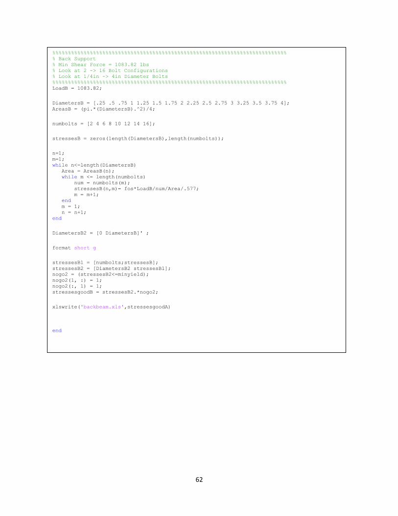
%%%%%%%%%%%%%%%%%%%%%%%%%%%%%%%%%%%%%%%%%%%%%%%%%%%%%%%%%%%%%%%%%%%%%%%%%%% % Back Support % Min Shear Force = 1083.82 lbs % Look at 2 -> 16 Bolt Configurations % Look at 1/4in -> 4in Diameter Bolts %%%%%%%%%%%%%%%%%%%%%%%%%%%%%%%%%%%%%%%%%%%%%%%%%%%%%%%%%%%%%%%%%%%%%%%%%%% LoadB = 1083.82;
DiametersB = [.25 .5 .75 1 1.25 1.5 1.75 2 2.25 2.5 2.75 3 3.25 3.5 3.75 4]; AreasB = (pi.*(DiametersB).^2)/4;
numbolts = [2 4 6 8 10 12 14 16];
stressesB = zeros(length(DiametersB),length(numbolts));
n=1; m=1; while n<=length(DiametersB) Area = AreasB(n); while m <= length(numbolts) num = numbolts(m); stressesB(n,m)= fos*LoadB/num/Area/.577; m = m+1; end m = 1; n = n+1; end
DiametersB2 = [0 DiametersB]' ;
format short g
stressesB1 = [numbolts;stressesB]; stressesB2 = [DiametersB2 stressesB1]; nogo2 = (stressesB2<=minyield); nogo2(1, :) = 1; nogo2(:, 1) = 1; stressesgoodB = stressesB2.*nogo2;
xlswrite('backbeam.xls',stressesgoodA)
end

63
Appendix B: Main Script for Welded Gear
clear;
close all;
clc;
%% Setting Snapshot Conditions
BeamWeight = 2604;
HeadWeight = 0.5*BeamWeight;
Ang = -0.6404; %angle off of horizontal position of walking beam, +-.6404
PumpForce = 500;
%% Dimensions of Beam / Weld
b = 12;
d = 28.8;
%% Determining Force
[F M] = Forces (BeamWeight, HeadWeight, Ang, PumpForce);
F = F / 1000; %converting to kips
M = M / 1000; %converting to kips
%% Setting a Table of Different Weld Thicknesses
h = [1;7/8;3/4;5/8;1/2;7/16;3/8;5/16;1/4;3/16;1/8;1/16];
%% Determining Stresses & Factors of Safety
[ Vert, Horiz, Side, Top, Box ] = Stresses( F, M, b, d, h);
%% Organizing Data
Ns = [Vert(:,4) Horiz(:,4) Side(:,4) Top(:,4) Box(:,4)];
As = [Vert(:,1) Horiz(:,1) Side(:,1) Top(:,1) Box(:,1)];

64
Appendix C: Helper Functions for Welded Joint
function [ VertParD, HorizParD, SideOpenD, TopOpenD, BoxD ] = Stresses( F, M, b, d, h)
[ VertPar, HorizPar, SideOpen, TopOpen, Box ] = BendingProperties( b, d, h );
%% Vertical Parallel
[VertParD] = Maths(F,M,VertPar);
%% Horizontal Parallel
[HorizParD] = Maths(F,M,HorizPar);
%% Three Sides, Side Open
[SideOpenD] = Maths(F,M,SideOpen);
%% Three Sides, Top Open
[TopOpenD] = Maths(F,M,TopOpen);
%% Box
[BoxD] = Maths(F,M,Box);
end
function [ VertPar, HorizPar, SideOpen, TopOpen, Box ] = BendingProperties( b, d, h )
%% Vertical Parallel
A = 1.414.*h.*d;
c = d./2 .*ones(size(h));
U = d.^3 ./6;
I = 0.707.*h.*U;
VertPar = [A,c,I];
%% Horizontal Parallel
A = 1.414.*h.*b;
U = b.*d.^2./2;
I = 0.707.*h.*U;
HorizPar = [A,c,I];
%% Three Sides, Side Open
A = 0.707.*h.*(2.*b + d);
U = d.^2./12.*(6.*b + d);
I = 0.707.*h.*U;
SideOpen = [A,c,I];
%% Box
A = 1.414.*h.*(b+d);
U = d.^2./6.*(3.*b+d);
I = 0.707.*h.*U;
Box = [A,c,I];
%% Three Sides, Top Open
A = 0.707.*h.*(b + 2.*d);
C = d.^2./(b+2.*d);
U = 2.*d.^3./6 - 2.*d.^2.*C + (b+2.*d).*C.^2;
I = 0.707.*h.*U;
c = C.*ones(size(h));
TopOpen = [A,c,I];
end

65
Appendix D: Input Options for Wire Rope
Type dmin dmax Weight
Factor
Sheave
Factor
Material Modulus of
Elasticity
Strength
6x7
haulage
.25 1.5 1.50 42 Monitor
Steel
14 100
Plow
Steel
14 88
Mild Plow
Steel
14 76
6x19
standard
hoisting
0.25 2.75 1.60 28 Monitor
Steel
12 106
Plow
Steel
12 93
Mild Plow
Steel
12 80
6x37
special
flexible
0.25 3.5 1.55 18 Monitor
Steel
11 100
Plow
Steel
11 88
8x19 extra
flexible
0.25 1.5 1.45 22 Monitor
Steel
10 92
Plow
Steel
10 80
66
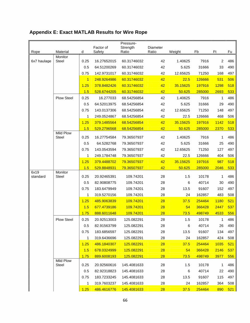
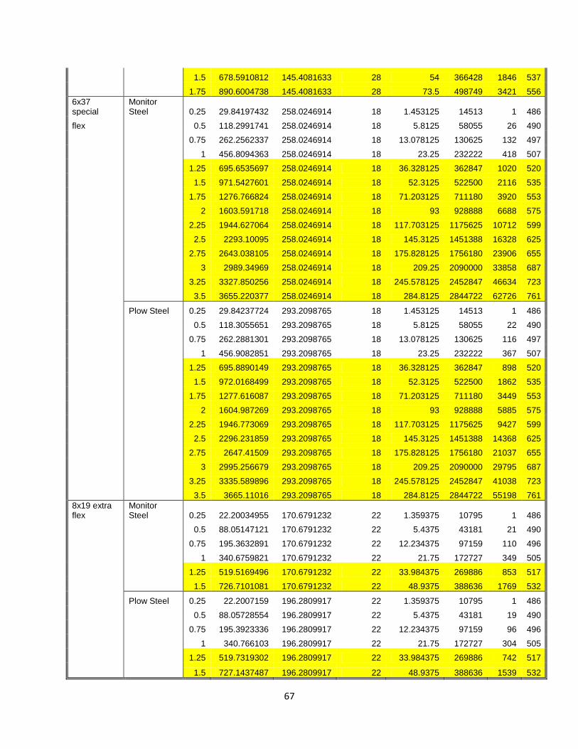
Appendix E: Exact MATLAB Results for Wire Rope
Rope Material d Factor of Safety
Pressure-Strength Ratio
Diameter Ratio Weight Fb Ft Fu
6x7 haulage Monitor Steel 0.25 16.27652015 60.31746032 42 1.40625 7916 2 486
0.5 64.51200269 60.31746032 42 5.625 31666 33 490
0.75 142.9731017 60.31746032 42 12.65625 71250 168 497
1 248.9264986 60.31746032 42 22.5 126666 531 506
1.25 378.8482426 60.31746032 42 35.15625 197916 1298 518
1.5 528.6744205 60.31746032 42 50.625 285000 2693 533
Plow Steel 0.25 16.277033 68.54256854 42 1.40625 7916 1 486
0.5 64.52013975 68.54256854 42 5.625 31666 29 490
0.75 143.0137306 68.54256854 42 12.65625 71250 148 497
1 249.0524867 68.54256854 42 22.5 126666 468 506
1.25 379.1485564 68.54256854 42 35.15625 197916 1142 518
1.5 529.2796568 68.54256854 42 50.625 285000 2370 533
Mild Plow Steel 0.25 16.27754584 79.36507937 42 1.40625 7916 1 486
0.5 64.5282768 79.36507937 42 5.625 31666 25 490
0.75 143.0543594 79.36507937 42 12.65625 71250 127 497
1 249.1784748 79.36507937 42 22.5 126666 404 506
1.25 379.4488702 79.36507937 42 35.15625 197916 987 518
1.5 529.8848931 79.36507937 42 50.625 285000 2046 533
6x19 standard
Monitor Steel 0.25 20.92465391 109.74201 28 1.5 10178 1 486
0.5 82.90808775 109.74201 28 6 40714 30 490
0.75 183.6479949 109.74201 28 13.5 91607 152 497
1 319.5270156 109.74201 28 24 162857 483 508
1.25 485.9063839 109.74201 28 37.5 254464 1180 521
1.5 677.4739186 109.74201 28 54 366428 2447 537
1.75 888.6011648 109.74201 28 73.5 498749 4533 556
Plow Steel 0.25 20.92513003 125.082291 28 1.5 10178 1 486
0.5 82.91563799 125.082291 28 6 40714 26 490
0.75 183.6856597 125.082291 28 13.5 91607 134 497
1 319.6436696 125.082291 28 24 162857 424 508
1.25 486.1840307 125.082291 28 37.5 254464 1035 521
1.5 678.0324999 125.082291 28 54 366428 2146 537
1.75 889.6008193 125.082291 28 73.5 498749 3977 556
Mild Plow Steel 0.25 20.92560616 145.4081633 28 1.5 10178 1 486
0.5 82.92318823 145.4081633 28 6 40714 22 490
0.75 183.7233245 145.4081633 28 13.5 91607 115 497
1 319.7603237 145.4081633 28 24 162857 364 508
1.25 486.4616776 145.4081633 28 37.5 254464 890 521
67
1.5 678.5910812 145.4081633 28 54 366428 1846 537
1.75 890.6004738 145.4081633 28 73.5 498749 3421 556
6x37 special
Monitor Steel 0.25 29.84197432 258.0246914 18 1.453125 14513 1 486
flex 0.5 118.2991741 258.0246914 18 5.8125 58055 26 490
0.75 262.2562337 258.0246914 18 13.078125 130625 132 497
1 456.8094363 258.0246914 18 23.25 232222 418 507
1.25 695.6535697 258.0246914 18 36.328125 362847 1020 520
1.5 971.5427601 258.0246914 18 52.3125 522500 2116 535
1.75 1276.766824 258.0246914 18 71.203125 711180 3920 553
2 1603.591718 258.0246914 18 93 928888 6688 575
2.25 1944.627064 258.0246914 18 117.703125 1175625 10712 599
2.5 2293.10095 258.0246914 18 145.3125 1451388 16328 625
2.75 2643.038105 258.0246914 18 175.828125 1756180 23906 655
3 2989.34969 258.0246914 18 209.25 2090000 33858 687
3.25 3327.850256 258.0246914 18 245.578125 2452847 46634 723
3.5 3655.220377 258.0246914 18 284.8125 2844722 62726 761
Plow Steel 0.25 29.84237724 293.2098765 18 1.453125 14513 1 486
0.5 118.3055651 293.2098765 18 5.8125 58055 22 490
0.75 262.2881301 293.2098765 18 13.078125 130625 116 497
1 456.9082851 293.2098765 18 23.25 232222 367 507
1.25 695.8890149 293.2098765 18 36.328125 362847 898 520
1.5 972.0168499 293.2098765 18 52.3125 522500 1862 535
1.75 1277.616087 293.2098765 18 71.203125 711180 3449 553
2 1604.987269 293.2098765 18 93 928888 5885 575
2.25 1946.773069 293.2098765 18 117.703125 1175625 9427 599
2.5 2296.231859 293.2098765 18 145.3125 1451388 14368 625
2.75 2647.41509 293.2098765 18 175.828125 1756180 21037 655
3 2995.256679 293.2098765 18 209.25 2090000 29795 687
3.25 3335.589896 293.2098765 18 245.578125 2452847 41038 723
3.5 3665.11016 293.2098765 18 284.8125 2844722 55198 761
8x19 extra flex
Monitor Steel 0.25 22.20034955 170.6791232 22 1.359375 10795 1 486
0.5 88.05147121 170.6791232 22 5.4375 43181 21 490
0.75 195.3632891 170.6791232 22 12.234375 97159 110 496
1 340.6759821 170.6791232 22 21.75 172727 349 505
1.25 519.5169496 170.6791232 22 33.984375 269886 853 517
1.5 726.7101081 170.6791232 22 48.9375 388636 1769 532
Plow Steel 0.25 22.2007159 196.2809917 22 1.359375 10795 1 486
0.5 88.05728554 196.2809917 22 5.4375 43181 19 490
0.75 195.3923336 196.2809917 22 12.234375 97159 96 496
1 340.766103 196.2809917 22 21.75 172727 304 505
1.25 519.7319302 196.2809917 22 33.984375 269886 742 517
1.5 727.1437487 196.2809917 22 48.9375 388636 1539 532
68
Appendix F: MATLAB Code for Wire Rope
function [results,forces] = wireRope(Fd,wF,sF,dmin,dmax,E,W,Su) % Author: Jennifer LaMere % Inputs: Fd = force desired % wF = weight factor % sF = sheave factor % dmin = minimum diameter % dmax = maximum diameter % E = modulus of elasticity % Su = ultimate tensile strength of material % W = weight at end of rope % Outputs: results = array of values % row1: diameter d % row2: factor of safety % row3: pressure-strength ratio % row 4: diameter ratio % row 5: rope weight % forces = array of forces % row1: Equivalent Bending Load % row2: Friction Force % row3: Tensile force
% Constants g=32.1; % ft/s^2 m = 1; % one rope l = 15; % length of rope a = 1; % Acceleraion of movement
% Setting up diameter ranges diams = dmin:.25:dmax; results = []; forces = [];
for index = 1:length(diams) d = diams(index); w = wF*(d^2); % weight D = sF*d; % sheave diameter sigma = E*(d/D); % solves for the stress Am = 0.38*(d^2); % area of metal Fb=sigma*Am; % Equivalent Bending Load P = (2*Fb)/(d*D); % bearing pressure Su2 = (2000*Fd)/(d*D); % ultimate tensile strenght of the wires Ff = ((P/Su2)*Su*d*D)/2; % frction force Ft = ((W/m)+w*l)/(1+(a/g)); % tensile stress force n = abs(Ff-Fb)/Ft; % Factor of Safety r = P/Su; % Pressure-Tensile Strength Ratio dr = D/d; % Diameter Ratio weight = w*l; % Overall weight of rope
new1 = [d,n,r,dr,weight]; new2 = [Fb,Ff,Ft]; results =[results;new1]; forces = [forces;new2]; end
end
69
Appendix G: Results for Shafts
70
Appendix H: MATLAB Code for Bearings
%% Bearing MATLAB Analysis % angular acceleration is tangential / radius
%% need to know % radial load F_d % desired life L_d % rated life L_R -- 10^6 % X_D = L_d / L_R % desired reliability R_d % Weibull parameters X_0, theta, b -- provided by manufacturer % Catalog load rating C_10 -- used to find suitable bearing from catalog
%% reliability
X_0 = .02; theta = 4.459; b = 1.483; L_D = 175 * 10^3; % kilo-hours L_R = 10^6; a_f = 3; % machinery with moderate impact [1.5 - 3.0] a = 3; % for ball bearing F_d = 3779.738; % radial load
X_D = L_D ./ L_R; R_d = exp(-((X_D - X_0) ./ (theta - X_0)).^b); C_10 = a_f .* F_d .* (X_D ./ (X_0 + (theta - X_0) .* (1 - R_d) .^ (1 ./
b))) .^ (1./a); newC_10 = (4.44822162 .* C_10) ./ 1000;
% round newC_10 up to 55.9 for chart % bore diameter = 65mm % outside diameter = 120 mm % width = 23 mm % fillet radius = 1.5 mm % shoulder diameter, ds = 74 mm, dh = 109 mm % C_10 = 55.9 % C_0 = 34
71
Resources:
"AISI 1018 Steel, Cold Drawn, High Temperature." Matweb.com. Matweb: Material
Property Data, 12 May 2011. Web. 07 Dec. 2012.
Carrick, H. Eighth European Congress on Fluid Machinery for the Oil, Gas, and
Petrochemical Industry: 31 October - 1 November 2002, Bilderberg Europa
Hotel, The Hague, The Netherlands. Bury St. Edmungs [u.a.: Professional
Engineering Publ., 2003. Print.
Norton, Robert L. Machine Design: An Integrated Approach. Upper Saddle River, NJ:
Pearson Prentice Hall, 2006. Print.
"Safety Factor of Statically Loaded Weld Joint." Wikihelp.autodesk.com. AutoDesk, 25
Mar. 2012. Web. 04 Dec. 2012.


![[INSERT PROJECT NAME]€¦ · Project name Project Number [Where applicable] Project Manager Project Controller Project location [Insert brief details of project location, including](https://img.pdfslide.net/doc/110x75/603496f741d854077e52cec0/insert-project-name-project-name-project-number-where-applicable-project-manager.jpg)