ME559(EE587) Nonlinear Control and Stability

Chapter 01: Introduction to Nonlinear Dynamical Systems

The topic of this course is analysis and control of nonlinear dynamical systems.

The term “nonlinear” is interpreted in primarily two ways, namely, “not linear” and

“not necessarily linear.” The latter meaning is intended here. There are several

important differences between linear systems and nonlinear systems. The main

difference is that a linear system is governed by the principle of superposition, i.e.,

L(cx + y) = cL(x) + L(y), where L is a linear operator; the scalar c belongs to

field of the vector space V ; and x, y ∈ V ; there are other differences that accrue

from inapplicability of the principle of superposition. For example, a closed-form

solution always exists for a set of finite-dimensional linear time-invariant (FDLTI)

differential equations; however, this may not be true for a set of nonliear ordinary

differential equations. Therefore, it is desirable to obtain a model that yields an

approximate solution of the governing equations of a nonlinear dynamical system

for the purpose of stability analysis and control.

1 Rudimentary Concepts

The general structure for a nonlinear dynamical system in the continuous-time

setting is represented as:

x(t) = f [t, x(t), u(t)] ∀t ≥ 0 (1)

where t ∈ R+ , [0,∞) denotes time; x(t) ∈ Rn, where n ∈ N , 1, 2, 3, · · · ,

denotes the state at time t; the input at time t is denoted by u(t) ∈ Rm with m ∈ N

and m ≤ n. Thus, f : R+ × Rn × R

m → Rn.

The discrete-time representation of Eq. (1) is a nonlinear map:

xk+1 = ϕk[xk, uk] ∀k (2)

where k ∈ N0 , 0, 1, 2, 3, · · · denotes instants of discrete time; xk ∈ Rn denotes

the state at instant k; the input uk ∈ Rm, where m ∈ N and m ≤ n, is the input

at instant k. Thus ϕk : Rn × Rm → R

n for all k ∈ N0. Next we introduce a few

definitions for commonly used terms.

Definition 1.1. A dynamical system in Eq. (1) (resp. Eq. (2)) is called forced

if the input u(t) serves as the forcing function. The system is called unforced if

u(t) = 0 ∀t ≥ 0 (resp. uk = 0 ∀k ≥ 0).

1

Definition 1.2. A dynamical system in Eq. (1) (resp. Eq. (2)) is called autonomous

if the function f does not explicitly depend on the time parameter t (resp. the

function ϕ does not explicitly depend on the time index k); otherwise the dynamical

system is called non-autonomous.

Definition 1.3. In an unforced dynamical system in Eq. (1) with u(t) = 0 ∀t ≥ 0

(resp. Eq. (2) with uk = 0 ∀k ≥ 0), a state xe at a time τ ≥ 0 (resp. xe at an

instant κ ≥ 0) is called an equilibrium if

f(t, xe) = 0 ∀t ≥ τ (resp. ϕ(k, xe) = 0 ∀k ≥ κ) (3)

Remark 1.1. Many properties that are taken as granted for linear (especially

linear time-invariant) systems do not hold for nonlinear systems, which is one of

the the major challenges in nonlinear systems analysis. A few of these properties

are elucidated below.

1. Existence of a solution; Eq. (1) (resp. Eq. (2)) has at least one solution.

2. Local existence and uniqueness of the solution; Eq. (1) (resp. Eq. (2)) has

exactly one solution for sufficiently small increment of time, i.e., (tf − to)

(resp. (kf − k0)) is small.

3. Global existence and uniqueness of the solution; Eq. (1) (resp. Eq. (2)) has

exactly one solution for all time t ∈ [0,∞) (resp. k ∈ N0)).

4. Well-posedness, i.e., a unique solution and its continuous dependence on the

initial condition: Eq. (1) (resp. Eq. (2)) for all time t ∈ [0,∞) (resp. k ∈N0) has exactly one solution that is continuously dependent on the initial

cobdition.

Example 1.1. Consider the scalar differential equation

x(t) = −sgn x(t) ∀t ≥ 0 and x(0) = 0

where

sgn θ ,

1 if θ ≥ 0

−1 if θ < 0

No continuously differentiable function x(t) exists as a solution of the above

differential equation. None of the above four statements hold.

Example 1.2. Consider the scalar differential equation

x(t) =1

2x(t)∀t ≥ 0 and x(0) = 0

The above equation yields two solutions, namely, x(t) = ±√t. Statement 1 is true

but the statement 2 is false.

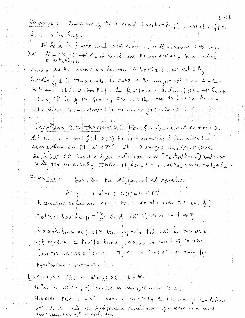
Example 1.3. Consider the scalar differential equation

x(t) = 1 + x2(t) ∀t ≥ 0 and x(0) = 0

2

over the interval [0, 1), the above equation has a unique solution x(t) = tan t, but

there is no continuously differentiable function x(t) defined over the entire interval

[0,∞) such that the above differential equation holds. This is so because as t → π/2,

the solution x(t) → ∞; this phenomenon is known as finite escape time, which

does not occur in linear systems. Locally, there is a unique solution but there is no

global solution.

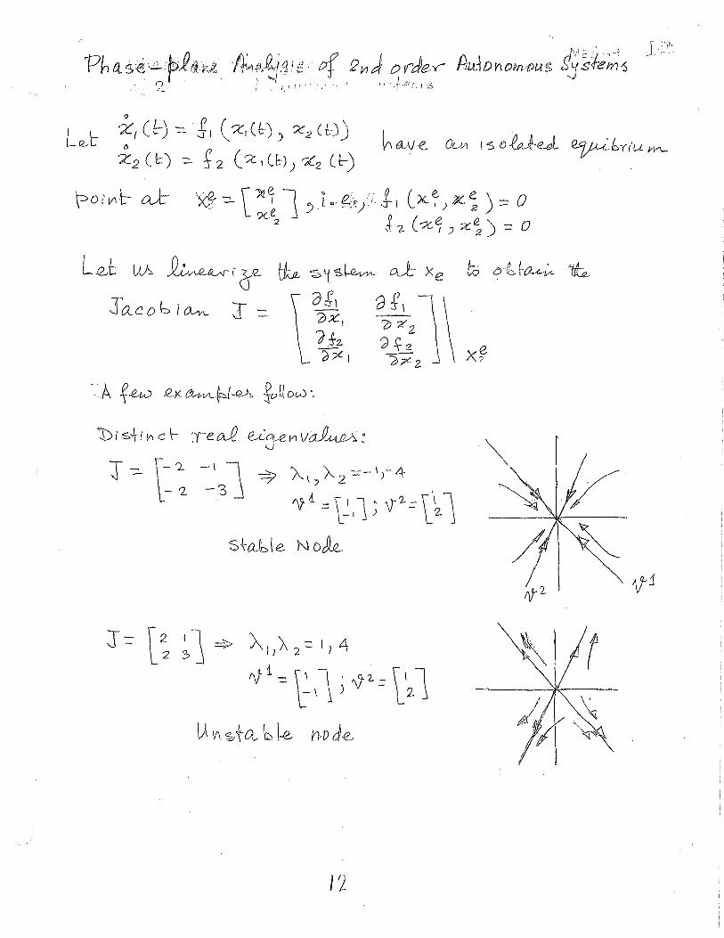
2 Second-order Nonlinear Dynamical Systems

Two-dimensional periodic orbits in R2 are special in the sense that they divide the

phase plane (in R2) into a region inside a closed curve and another region outside

it. This fact leads to the development of criteria for detection of presence or ab-

sence of periodic orbits for second-order systems. Commonly known are Bendixson,

Poincare-Bendixson, and Index criteria that are briefly introduced in this section.

Example 2.1. Hill’s equation (e.g., oscillations in a varying-stiffness coil)

y(t) + ω2(t)y(t) = 0

where ω is T -periodic, i.e., ω(t) = ω(t+T ) for a given T ∈ (0,∞). Notice that this

is a time-varying linear differential equation.

Let ω2(t) = [1 + ε cos(Ωt)]ω2o , which implies that

y(t) + [1 + ε cos(Ωt)]ω2o ] y(t) = 0

This known as Mathieu equation, for which an example is a child moving his/her

legs while swinging on a swing set. We often classify this type of problems as

parametrically excited oscillations.

Example 2.2. Unforced Duffing equation (e.g., oscillations of a nonlinear spring)

y(t) + α1y(t) + α3y3(t) = 0 for t ≥ 0; initial condition y(0) = 1, y(0) = 0

The above equation yields approximate solutions in the following range:

y(t, α3) ∼ cos(t) =[3

8t sin(t)+

1

32

(

cos(t)−cos(3t))

]

α3 for α1 = 1 and 0 < α3 ≪ 1.

Example 2.3. Forced Duffing equation (e.g., chaotic motion)

y(t)+βy(t)+α1y(t)+α3y3(t) = A cos(Ω t) for t ≥ 0; initial condition y(0) = 1, y(0) = 0.

Simulate the above equation for the following parameters to yield chaotic motion:

β = 0.05, α1 = 0, α3 = 1, A = 7.5, and Ω = 1.

Example 2.4. Unforced van der Pol equation (e.g., sustained oscillations)

y(t) + µ(y2(t)− 1)ω0 y(t) + ω20y(t) = 0 for t ≥ 0

For µ > 0, the above equation yields a stable limit cycle and the approximate radius

of the limit cycle is 2 if ω0 = 1.

3

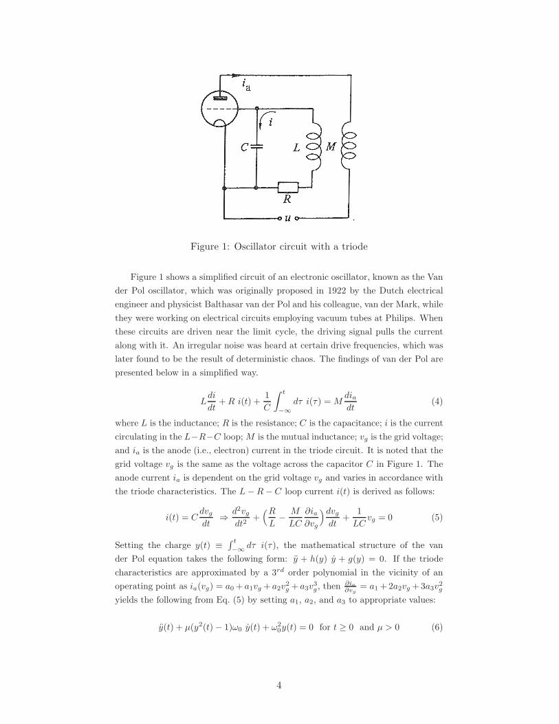
Figure 1: Oscillator circuit with a triode

Figure 1 shows a simplified circuit of an electronic oscillator, known as the Van

der Pol oscillator, which was originally proposed in 1922 by the Dutch electrical

engineer and physicist Balthasar van der Pol and his colleague, van der Mark, while

they were working on electrical circuits employing vacuum tubes at Philips. When

these circuits are driven near the limit cycle, the driving signal pulls the current

along with it. An irregular noise was heard at certain drive frequencies, which was

later found to be the result of deterministic chaos. The findings of van der Pol are

presented below in a simplified way.

Ldi

dt+R i(t) +

1

C

∫ t

−∞

dτ i(τ) = Mdiadt

(4)

where L is the inductance; R is the resistance; C is the capacitance; i is the current

circulating in the L−R−C loop; M is the mutual inductance; vg is the grid voltage;

and ia is the anode (i.e., electron) current in the triode circuit. It is noted that the

grid voltage vg is the same as the voltage across the capacitor C in Figure 1. The

anode current ia is dependent on the grid voltage vg and varies in accordance with

the triode characteristics. The L−R− C loop current i(t) is derived as follows:

i(t) = Cdvgdt

⇒ d2vgdt2

+(R

L− M

LC

∂ia∂vg

)dvgdt

+1

LCvg = 0 (5)

Setting the charge y(t) ≡∫ t

−∞dτ i(τ), the mathematical structure of the van

der Pol equation takes the following form: y + h(y) y + g(y) = 0. If the triode

characteristics are approximated by a 3rd order polynomial in the vicinity of an

operating point as ia(vg) = a0 + a1vg + a2v2g + a3v

3g , then

∂ia∂vg

= a1+2a2vg +3a3v2g

yields the following from Eq. (5) by setting a1, a2, and a3 to appropriate values:

y(t) + µ(y2(t)− 1)ω0 y(t) + ω20y(t) = 0 for t ≥ 0 and µ > 0 (6)

4