Embed Size (px)
Citation preview

IIT Kanpur
ME698S – Machining Dynamics
Dr. Mohit Law
Oblique Cutting

IIT Kanpur
Orthogonal and oblique cutting geometry
2
Cutting velocity is inclined at an acute angle 𝑖 to the cutting edge
Cutting velocity is perpendicular to cutting edge
Altintas, Mfg. Automation
IIT Kanpur
Oblique cutting geometry
3
Considerations: 1. Cutting edge is perfectly sharp
and no edge rubbing 2. Continuous chip with no built up-
edge 3. Tool subjected to 3D system of
cutting forces because of angle of obliquity, 𝑖
4. Non-plane strain deformation (treated however as a modified plane strain problem)
5. Uniform stress distribution on shear plane

IIT Kanpur
Recalling orthogonal cutting
4
• Plane normal to the cutting edge, and aligned
with the cutting velocity 𝑉 is the normal
plane 𝑃𝑛
• Because of plane strain deformation (and no
side spread), shearing and chip motion are
identical on all normal planes ∥ to 𝑉and ⊥ to
the cutting edge
• Hence, all velocities 𝑉, 𝑉𝑠, and 𝑉𝑐 are all ⊥ to
the cutting edge and lie in the velocity plane
𝑃𝑣 ∥ to or coincident with 𝑃𝑛
• Resultant force 𝐹𝑐, along with other forces
acting on the shear and chip-rake face contact
zone, also lie in the normal plane 𝑃𝑛
• No cutting force ⊥ to 𝑃𝑛, and edge forces = 0
Normal plane 𝑃𝑛

IIT Kanpur
Oblique cutting geometry
5
• Cutting velocity is inclined at an acute
angle 𝑖 to the cutting edge, hence
direction of shear, friction, chip flow, and
resultant force vectors have components
in all there Cartesian coordinates 𝑥, 𝑦, 𝑧
• Plane normal to the cutting edge, and
inclined at an acute angle 𝑖 with the
cutting velocity 𝑉 is the normal plane 𝑃𝑛
• 𝑥 is ⊥ to the cutting edge, but lies on cut
surface 𝑦 is aligned with cutting edge 𝑧 is
⊥ to 𝑥𝑦 plane
• Important planes are shear plane, rake
face, cut surface 𝑥𝑦 normal plane 𝑥𝑧 (or
𝑃𝑛), and the velocity plane 𝑃𝑣

IIT Kanpur
Oblique cutting geometry
6
• Assume that mechanics of oblique
cutting in the normal plane 𝑃𝑛 are
equivalent to orthogonal cutting. Hence
project velocities and forces into normal
plane
• Angle between shear and 𝑥𝑦 plane is the
normal shear angle - 𝜙𝑛
• Shear velocity lies on shear plane but
makes an oblique shear angle - 𝜙𝑖 with
the vector normal to the cutting edge on
the normal plane
• Sheared chip moves over rake face with a
chip flow angle of - 𝜂 measured from a
vector on the rake face but normal to
cutting edge
• Angle between 𝑧 axis and normal vector
on rake face is the normal rake angle - 𝛼𝑛

IIT Kanpur
Force diagram – oblique cutting
7
• Friction force on the rake face 𝐹 𝑢 and
normal force to the rake 𝐹 𝑣 form a resultant
cutting force 𝐹 𝑐 with a friction angle 𝛽𝑎
• This resultant 𝐹 𝑐 has an acute projection angle of 𝜃𝑖 with the normal plane 𝑃𝑛, which in turn has an in-plane angle of 𝜃𝑛 + 𝛼𝑛
with the normal force 𝐹 𝑣 • Where 𝜃𝑛 is the angle between the 𝑥 axis
and the projection of 𝐹 𝑐 on 𝑃𝑛
𝐹𝑢 = 𝐹𝑐 sin 𝛽𝑎 = 𝐹sin 𝜃𝑖
sin 𝜂→ sin 𝜃𝑖 = sin 𝛽𝑎 sin 𝜂
𝐹𝑢 = 𝐹𝑣 tan 𝛽𝑎 = 𝐹𝑣
tan 𝜃𝑛 + 𝛼𝑛
cos 𝜂→ tan 𝜃𝑛 + 𝛼𝑛 = tan 𝛽𝑎 cos 𝜂
Can derive the following geometric relations

IIT Kanpur
Velocity diagram – oblique cutting
8
𝑉 = 𝑉 cos 𝑖 , 𝑉 sin 𝑖 , 0 ,
𝑉𝑐 = 𝑉𝑐 cos 𝜂 sin 𝛼𝑛 , 𝑉𝑐 sin 𝜂 , 𝑉𝑐 cos 𝜂 cos𝛼𝑛 ,
𝑉𝑠 = −𝑉𝑠 cos𝜙𝑖 cos𝜙𝑛 , −𝑉𝑠 sin𝜙𝑖 , 𝑉𝑠 cos𝜙𝑖 sin𝜙𝑛
Defining each velocity vector by its Cartesian components:
Eliminate 𝑉, 𝑉𝑐, and 𝑉𝑠
𝑉𝑠 = 𝑉𝑐 − 𝑉
rearranging, following geometric relation between shear and chip flow directions
tan 𝜂 =tan 𝑖 cos 𝜙𝑛 − 𝛼𝑛 − cos𝛼𝑛 tan𝜙𝑖
sin𝜙𝑛
IIT Kanpur
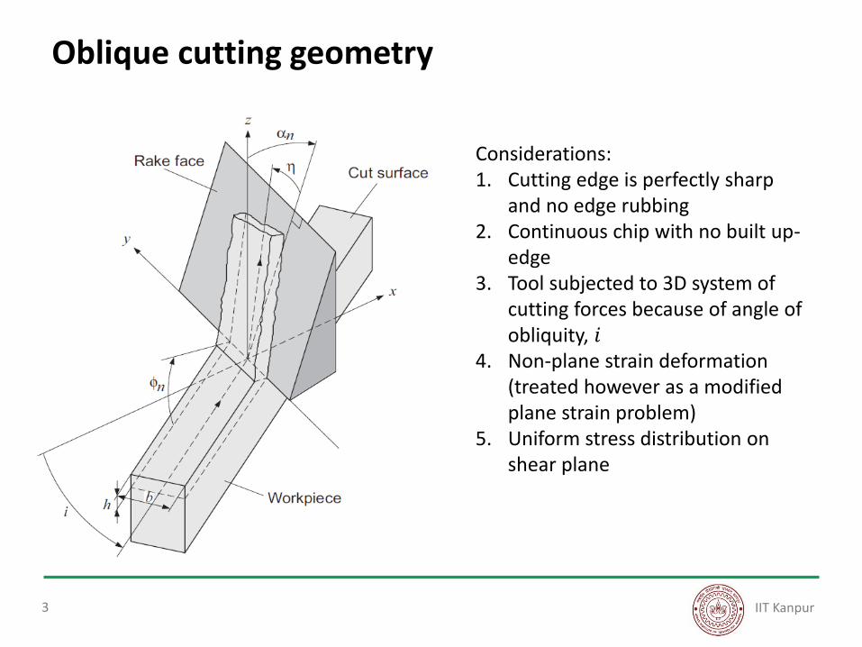
Solving for oblique cutting parameters
9
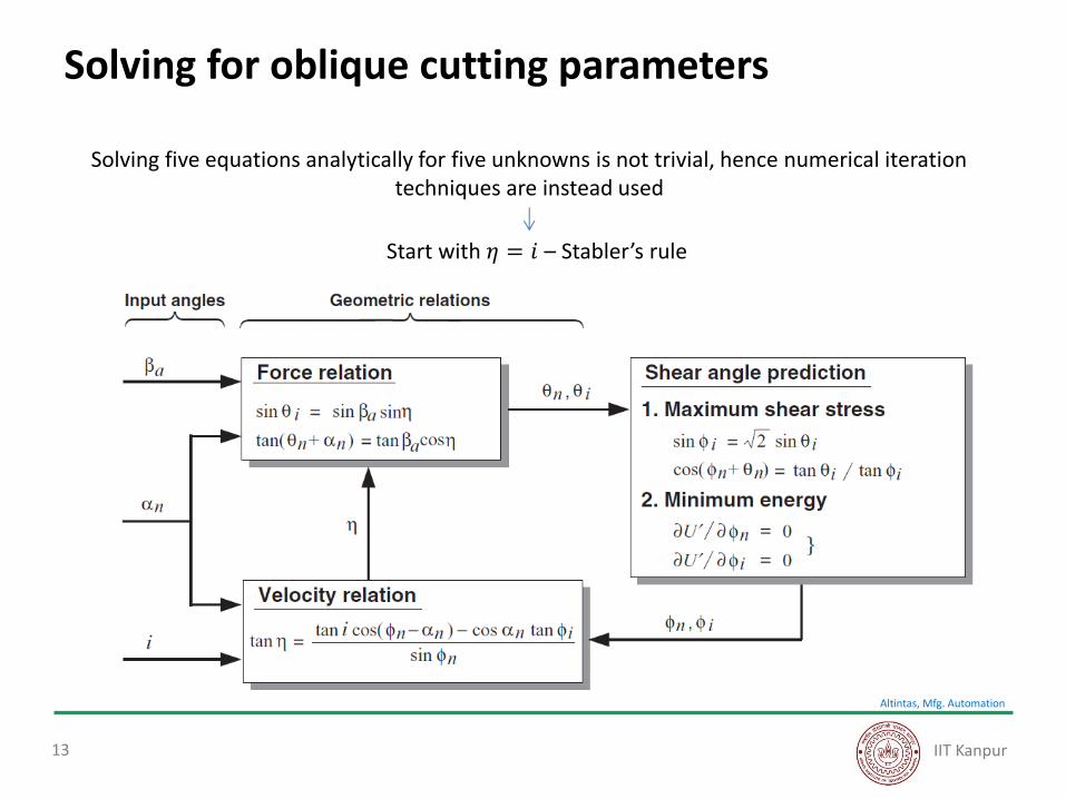
sin 𝜃𝑖 = sin 𝛽𝑎 sin 𝜂
tan 𝜃𝑛 + 𝛼𝑛 = tan 𝛽𝑎 cos 𝜂
tan 𝜂 =tan 𝑖 cos 𝜙𝑛 − 𝛼𝑛 − cos𝛼𝑛 tan𝜙𝑖
sin𝜙𝑛
Five unknown oblique cutting parameters that define the directions of resultant force 𝜃𝑛, 𝜃𝑖 , shear velocity 𝜙𝑛, 𝜙𝑖 , and chip flow 𝜂 .
Three equations – what to do? Empirical, model based?

IIT Kanpur
Minimum energy principle
10
Recall – Merchant’s approach to predict shear angle by applying the principle of minimum energy principle to orthogonal cutting
𝑃𝑡𝑐 = 𝑉𝐹𝑡𝑐 Power consumed during cutting: 𝑑𝑃𝑡𝑐
𝑑𝜙𝑐= 0 → 𝜙𝑐 =
𝜋
4−
𝛽𝑎 − 𝛼𝑟
2
𝐹𝑠 = 𝐹𝑐 cos 𝜃𝑛 + 𝜙𝑛 cos 𝜃𝑖 cos𝜙𝑖
+ sin 𝜃𝑖 sin𝜙𝑖
Extend the same principle here for oblique cutting
First need shear force (primary power consumption is during shearing)
Represent shear force as a
projection of resultant 𝐹 𝑐 in the direction of shear:
IIT Kanpur
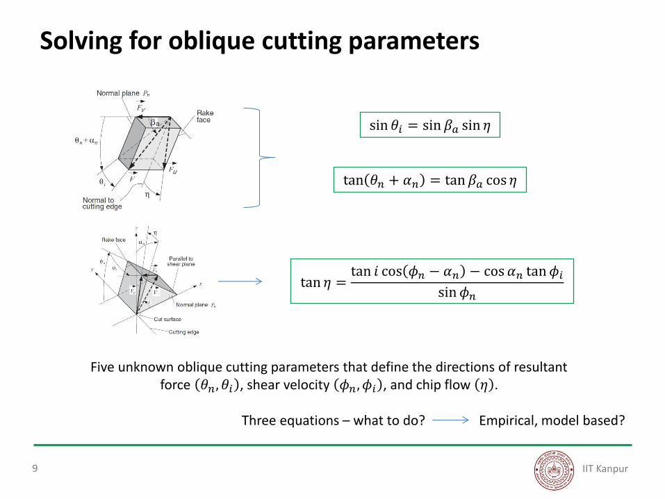
Minimum energy principle
11
𝐹𝑠 = 𝜏𝑠𝐴𝑠 = 𝜏𝑠 𝑏
cos 𝑖
ℎ
sin 𝜙𝑛
Representing shear force as a product of shear stress and shear
plane area 𝐹𝑠 = 𝐹𝑐 cos 𝜃𝑛 + 𝜙𝑛 cos 𝜃𝑖 cos𝜙𝑖 + sin 𝜃𝑖 sin𝜙𝑖
Represent shear force as a projection of resultant
𝐹 𝑐 in the direction of shear: or
𝐹𝑐 =𝜏𝑠𝑏ℎ
cos 𝜃𝑛 + 𝜙𝑛 cos 𝜃𝑖 cos𝜙𝑖 + sin 𝜃𝑖 sin𝜙𝑖 cos 𝑖 sin 𝜙𝑛
𝑃𝑡𝑐 = 𝑉𝐹𝑡𝑐 Power consumed
during cutting: 𝑃𝑡𝑐 = 𝐹𝑐 cos 𝜃𝑖 cos 𝜃𝑛 cos 𝑖 + sin 𝜃𝑖 sin 𝑖 𝑉
In terms of 𝐹𝑐
(a)
(b)
Substitute (a) into (b)
𝑃𝑡′ =
𝑃𝑡𝑐
𝑉𝜏𝑠𝑏ℎ=
cos𝜃𝑛 + tan 𝜃𝑖 tan 𝑖
cos 𝜃𝑛 + 𝜙𝑛 cos𝜙𝑖 + tan 𝜃𝑖 sin 𝜙𝑖 sin𝜙𝑛

IIT Kanpur
Minimum energy principle
12
Power 𝑃𝑡′: 𝑃𝑡
′ =𝑃𝑡𝑐
𝑉𝜏𝑠𝑏ℎ=
cos𝜃𝑛 + tan 𝜃𝑖 tan 𝑖
cos 𝜃𝑛 + 𝜙𝑛 cos𝜙𝑖 + tan 𝜃𝑖 sin𝜙𝑖 sin 𝜙𝑛
Minimum energy principle dictates that the cutting power must be minimum for a unique shear angle solution. Since 𝜏𝑠, 𝑏, ℎ, and 𝑉 is constant, and since the direction of shear is characterized
by 𝜙𝑛 and 𝜙𝑖, we have:
𝜕𝑃𝑡′
𝜕𝜙𝑛= 0;
𝜕𝑃𝑡′
𝜕𝜙𝑖= 0
sin 𝜃𝑖 = sin 𝛽𝑎 sin 𝜂
tan 𝜃𝑛 + 𝛼𝑛 = tan 𝛽𝑎 cos 𝜂
tan 𝜂 =tan 𝑖 cos 𝜙𝑛 − 𝛼𝑛 − cos𝛼𝑛 tan𝜙𝑖
sin𝜙𝑛
Which gives us two additional equations, in addition to the earlier three to solve for five unknowns
Recalling the earlier three
(1)
(2)
(3)
(4-5)
IIT Kanpur
Solving for oblique cutting parameters
13
Solving five equations analytically for five unknowns is not trivial, hence numerical iteration techniques are instead used
Start with 𝜂 = 𝑖 – Stabler’s rule
Altintas, Mfg. Automation

IIT Kanpur
Empirical solutions to oblique cutting parameters
14
Armarego & Whitfield
Three equations five unknowns (𝜙𝑛, 𝜙𝑖, 𝜂, 𝜃𝑖, 𝜃𝑛)
sin 𝜃𝑖 = sin 𝛽𝑎 sin 𝜂
tan 𝜃𝑛 + 𝛼𝑛 = tan 𝛽𝑎 cos 𝜂
tan 𝜂 =tan 𝑖 cos 𝜙𝑛 − 𝛼𝑛 − cos𝛼𝑛 tan𝜙𝑖
sin𝜙𝑛
(1)
(2)
(3)
Assume: 1. Shear velocity is collinear with shear force – from Stabler’s work 2. Chip length ratio in oblique is same as in orthogonal – from experiments
tan 𝜙𝑛 + 𝛽𝑛 =cos𝛼𝑛 tan 𝑖
tan 𝜂 − sin 𝛼𝑛 tan 𝑖 𝛽𝑛 = 𝜃𝑛 + 𝛼𝑛
tan 𝛽𝑛 = tan𝛽𝑎 cos 𝜂 𝜙𝑛 = tan−1𝑟𝑐 cos 𝜂 / cos 𝑖 cos𝛼𝑛
1 − 𝑟𝑐 cos 𝜂 / cos 𝑖 sin 𝛼𝑛
Combine Eq. (1) to (3): (1a)
(2a) (3a)
Solve Eq. (1a) – (3a) numerically to get 𝜂, 𝜙𝑛 and 𝛽𝑛.
Or assume 𝜂 = 𝑖 (Stabler’s rule) for analytical solution

IIT Kanpur
Prediction of cutting forces
15
𝐹𝑟𝑐 = 𝐹𝑐 sin 𝜃𝑖 cos 𝜃𝑖 − cos 𝜃𝑖 cos 𝜃𝑛 sin 𝑖 =𝜏𝑠𝑏ℎ tan𝜃𝑖 − cos 𝜃𝑛 tan 𝑖
cos 𝜃𝑛 + 𝜙𝑛 cos𝜙𝑖 + tan𝜃𝑖 sin𝜙𝑖 sin𝜙𝑛
𝐹𝑡𝑐 = 𝐹𝑐 cos𝜃𝑖 cos𝜃𝑛 cos𝜃𝑖 + sin 𝜃𝑖 sin 𝑖 =𝜏𝑠𝑏ℎ cos𝜃𝑛 + tan 𝜃𝑖 tan 𝑖
cos 𝜃𝑛 + 𝜙𝑛 cos𝜙𝑖 + tan 𝜃𝑖 sin𝜙𝑖 sin𝜙𝑛
𝐹𝑓𝑐 = 𝐹𝑐 cos 𝜃𝑖 sin 𝜃𝑛 =𝜏𝑠𝑏ℎ sin 𝜃𝑛
cos 𝜃𝑛 + 𝜙𝑛 cos𝜙𝑖 + tan 𝜃𝑖 sin𝜙𝑖 sin𝜙𝑛
Cutting force components are derived as projections of resultant cutting force 𝐹𝑐 after subtracting the edge components 𝐹𝑒 from measured resultant 𝐹
Force in direction of cutting speed
Expressing force components as a 𝑓 𝜏𝑠, 𝜙𝑛, 𝜙𝑖 , 𝜃𝑖, 𝜃𝑛 :
Force in direction of thrust
Force in direction of normal

IIT Kanpur
Prediction of cutting forces
16
𝐹𝑡 = 𝐾𝑡𝑐𝑏ℎ + 𝐾𝑡𝑒𝑏; 𝐹𝑓 = 𝐾𝑓𝑐𝑏ℎ + 𝐾𝑓𝑒𝑏;
𝐹𝑟 = 𝐾𝑟𝑐𝑏ℎ + 𝐾𝑟𝑒𝑏;
𝐾𝑡𝑐 =𝜏𝑠 cos 𝜃𝑛 + tan 𝜃𝑖 tan 𝑖
cos 𝜃𝑛 + 𝜙𝑛 cos 𝜙𝑖 + tan 𝜃𝑖 sin𝜙𝑖 sin𝜙𝑛
𝐾𝑓𝑐 =𝜏𝑠 sin 𝜃𝑛
cos 𝜃𝑛 + 𝜙𝑛 cos 𝜙𝑖 + tan 𝜃𝑖 sin𝜙𝑖 sin𝜙𝑛
𝐾𝑟𝑐 =𝜏𝑠𝑏ℎ tan 𝜃𝑖 − cos 𝜃𝑛 tan 𝑖
cos 𝜃𝑛 + 𝜙𝑛 cos 𝜙𝑖 + tan 𝜃𝑖 sin𝜙𝑖 sin𝜙𝑛
𝐹𝑟𝑐 =𝜏𝑠𝑏ℎ tan 𝜃𝑖 − cos 𝜃𝑛 tan 𝑖
cos 𝜃𝑛 + 𝜙𝑛 cos 𝜙𝑖 + tan 𝜃𝑖 sin𝜙𝑖 sin𝜙𝑛
𝐹𝑡𝑐 =𝜏𝑠𝑏ℎ cos 𝜃𝑛 + tan 𝜃𝑖 tan 𝑖
cos 𝜃𝑛 + 𝜙𝑛 cos 𝜙𝑖 + tan 𝜃𝑖 sin𝜙𝑖 sin𝜙𝑛 𝐹𝑓𝑐 =
𝜏𝑠𝑏ℎ sin 𝜃𝑛
cos 𝜃𝑛 + 𝜙𝑛 cos 𝜙𝑖 + tan 𝜃𝑖 sin𝜙𝑖 sin𝜙𝑛
Force in direction of cutting speed
Expressing force components as a 𝑓 𝜏𝑠, 𝜙𝑛, 𝜙𝑖 , 𝜃𝑖, 𝜃𝑛 :
Force in direction of thrust
Force in direction of normal
Rewriting forces in the convenient form of:

IIT Kanpur
Prediction of cutting forces – Armarego’s model
17
𝐹𝑟𝑐 =𝜏𝑠𝑏ℎ tan 𝜃𝑖 − cos 𝜃𝑛 tan 𝑖
cos 𝜃𝑛 + 𝜙𝑛 cos 𝜙𝑖 + tan 𝜃𝑖 sin𝜙𝑖 sin𝜙𝑛
𝐹𝑡𝑐 =𝜏𝑠𝑏ℎ cos 𝜃𝑛 + tan 𝜃𝑖 tan 𝑖
cos 𝜃𝑛 + 𝜙𝑛 cos 𝜙𝑖 + tan 𝜃𝑖 sin𝜙𝑖 sin𝜙𝑛 𝐹𝑓𝑐 =
𝜏𝑠𝑏ℎ sin 𝜃𝑛
cos 𝜃𝑛 + 𝜙𝑛 cos 𝜙𝑖 + tan 𝜃𝑖 sin𝜙𝑖 sin𝜙𝑛
Force in direction of cutting speed
Expressing force components as a 𝑓 𝜏𝑠, 𝜙𝑛, 𝜙𝑖 , 𝜃𝑖, 𝜃𝑛 :
Force in direction of thrust
Force in direction of normal
Using Armarego’s classical oblique cutting model,
forces are transformed in
terms of 𝑓 𝜏𝑠, 𝛽𝑛,𝜙𝑛𝛼𝑛,𝜂
𝐹𝑡 = 𝑏ℎ𝜏𝑠
sin𝜙𝑛
cos 𝛽𝑛 − 𝛼𝑛 + tan 𝑖 tan 𝜂 sin 𝛽𝑛
𝑐𝑜𝑠2 𝜙𝑛 + 𝛽𝑛 − 𝛼𝑛 + 𝑡𝑎𝑛2𝜂𝑠𝑖𝑛2𝛽𝑛
𝐹𝑓 = 𝑏ℎ𝜏𝑠
sin𝜙𝑛 cos 𝑖
sin 𝛽𝑛 − 𝛼𝑛
𝑐𝑜𝑠2 𝜙𝑛 + 𝛽𝑛 − 𝛼𝑛 + 𝑡𝑎𝑛2𝜂𝑠𝑖𝑛2𝛽𝑛
𝐹𝑟 = 𝑏ℎ𝜏𝑠
sin𝜙𝑛
cos 𝛽𝑛 − 𝛼𝑛 cos 𝛽𝑛 − 𝛼𝑛 tan 𝑖 −tan 𝜂 sin 𝛽𝑛
𝑐𝑜𝑠2 𝜙𝑛 + 𝛽𝑛 − 𝛼𝑛 + 𝑡𝑎𝑛2𝜂𝑠𝑖𝑛2𝛽𝑛
Armarego’s force model

IIT Kanpur
Oblique cutting – force coefficients
18
𝐹𝑡 = 𝑏ℎ𝜏𝑠
sin𝜙𝑛
cos 𝛽𝑛 − 𝛼𝑛 + tan 𝑖 tan 𝜂 sin 𝛽𝑛
𝑐𝑜𝑠2 𝜙𝑛 + 𝛽𝑛 − 𝛼𝑛 + 𝑡𝑎𝑛2𝜂𝑠𝑖𝑛2𝛽𝑛
𝐹𝑓 = 𝑏ℎ𝜏𝑠
sin𝜙𝑛 cos 𝑖
sin 𝛽𝑛 − 𝛼𝑛
𝑐𝑜𝑠2 𝜙𝑛 + 𝛽𝑛 − 𝛼𝑛 + 𝑡𝑎𝑛2𝜂𝑠𝑖𝑛2𝛽𝑛
𝐹𝑟 = 𝑏ℎ𝜏𝑠
sin𝜙𝑛
cos 𝛽𝑛 − 𝛼𝑛 cos 𝛽𝑛 − 𝛼𝑛 tan 𝑖 −tan 𝜂 sin 𝛽𝑛
𝑐𝑜𝑠2 𝜙𝑛 + 𝛽𝑛 − 𝛼𝑛 + 𝑡𝑎𝑛2𝜂𝑠𝑖𝑛2𝛽𝑛
𝐾𝑡𝑐 =𝜏𝑠
sin𝜙𝑛
cos 𝛽𝑛 − 𝛼𝑛 + tan 𝑖 tan 𝜂 sin 𝛽𝑛
𝑐𝑜𝑠2 𝜙𝑛 + 𝛽𝑛 − 𝛼𝑛 + 𝑡𝑎𝑛2𝜂𝑠𝑖𝑛2𝛽𝑛
𝐾𝑓𝑐 =𝜏𝑠
sin𝜙𝑛 cos 𝑖
sin 𝛽𝑛 − 𝛼𝑛
𝑐𝑜𝑠2 𝜙𝑛 + 𝛽𝑛 − 𝛼𝑛 + 𝑡𝑎𝑛2𝜂𝑠𝑖𝑛2𝛽𝑛
𝐾𝑟𝑐 =𝜏𝑠
sin𝜙𝑛
cos 𝛽𝑛 − 𝛼𝑛 cos 𝛽𝑛 − 𝛼𝑛 tan 𝑖 −tan 𝜂 sin 𝛽𝑛
𝑐𝑜𝑠2 𝜙𝑛 + 𝛽𝑛 − 𝛼𝑛 + 𝑡𝑎𝑛2𝜂𝑠𝑖𝑛2𝛽𝑛
𝐹𝑡 = 𝐾𝑡𝑐𝑏ℎ + 𝐾𝑡𝑒𝑏; 𝐹𝑓 = 𝐾𝑓𝑐𝑏ℎ + 𝐾𝑓𝑒𝑏;
𝐹𝑟 = 𝐾𝑟𝑐𝑏ℎ + 𝐾𝑟𝑒𝑏;
Using Armarego’s classical oblique cutting model,
forces are transformed as
Armarego’s force model

IIT Kanpur
Practical approach – for force prediction
19
𝐾𝑡𝑐 =𝜏𝑠
sin 𝜙𝑛
cos 𝛽𝑛 − 𝛼𝑛 + tan 𝑖 tan 𝜂 sin 𝛽𝑛
𝑐𝑜𝑠2 𝜙𝑛 + 𝛽𝑛 − 𝛼𝑛 + 𝑡𝑎𝑛2𝜂𝑠𝑖𝑛2𝛽𝑛
𝐾𝑓𝑐 =𝜏𝑠
sin 𝜙𝑛 cos 𝑖
sin 𝛽𝑛 − 𝛼𝑛
𝑐𝑜𝑠2 𝜙𝑛 + 𝛽𝑛 − 𝛼𝑛 + 𝑡𝑎𝑛2𝜂𝑠𝑖𝑛2𝛽𝑛
𝐾𝑟𝑐 =𝜏𝑠
sin 𝜙𝑛
cos 𝛽𝑛 − 𝛼𝑛 cos 𝛽𝑛 − 𝛼𝑛 tan 𝑖 −tan 𝜂 sin 𝛽𝑛
𝑐𝑜𝑠2 𝜙𝑛 + 𝛽𝑛 − 𝛼𝑛 + 𝑡𝑎𝑛2𝜂𝑠𝑖𝑛2𝛽𝑛
• Evaluate shear angle 𝜙𝑐, friction angle 𝛽𝑎, and shear stress 𝜏𝑠 from orthogonal cutting tests
• Assume orthogonal shear angle equals normal shear angle, i.e. 𝜙𝑐 ≡ 𝜙𝑛
• Assume normal rake angle equals rake angle in orthogonal cutting, i.e. 𝛼𝑟 ≡ 𝛼𝑛
• Assume chip flow angle equals oblique angle (Stabler’s rule), i.e. 𝜂 ≡ 𝑖
• Assume friction angle in orthognal cutting is same as in oblique, i.e. 𝛽𝑎 ≡ 𝛽𝑛
• Assume shear stress remains the same in orthogonal and oblique cutting
𝐹𝑡 = 𝐾𝑡𝑐𝑏ℎ + 𝐾𝑡𝑒𝑏; 𝐹𝑓 = 𝐾𝑓𝑐𝑏ℎ + 𝐾𝑓𝑒𝑏;
𝐹𝑟 = 𝐾𝑟𝑐𝑏ℎ + 𝐾𝑟𝑒𝑏;
Evaluate cutting force coefficients
Predict cutting forces

IIT Kanpur
Yet another practical approach
20
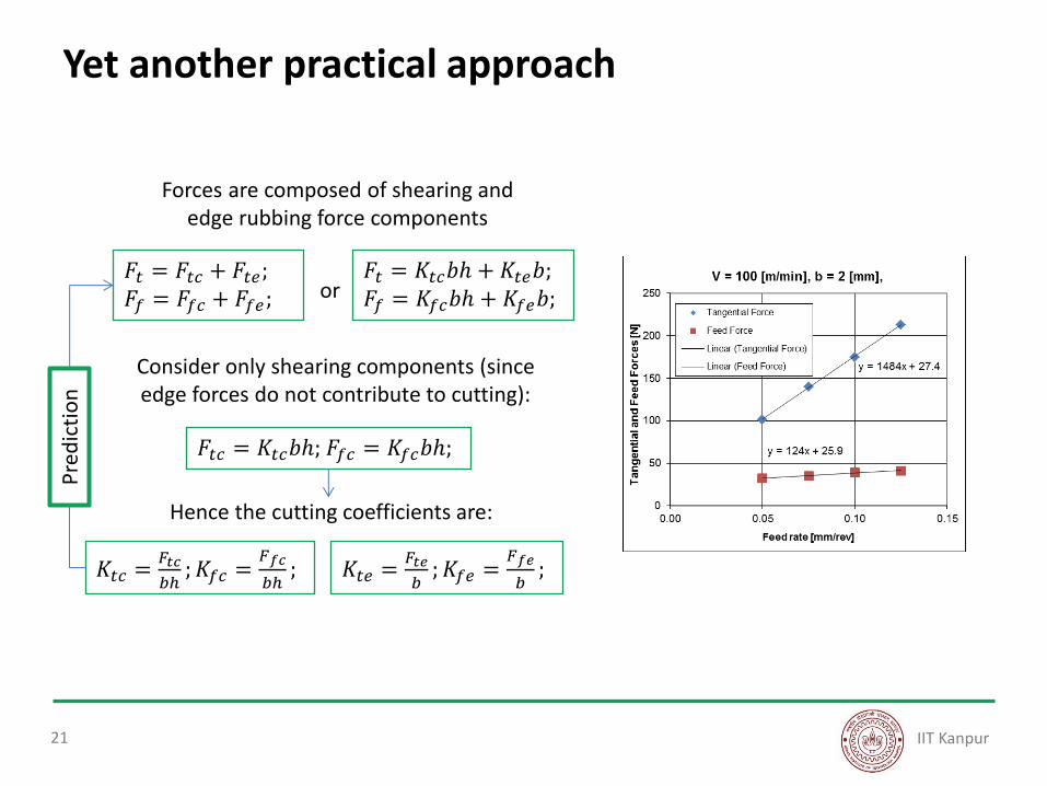
Feed Rate Measured Measured
Test No: h [mm/rev] Ftc [N] Ffc [N] 1 0.050 101 32
2 0.075 140 35
3 0.100 175 39
4 0.125 213 41
Conduct a dedicated series of tests at different feed rates and identify coefficients directly for the tool-workpiece-cutting parameter combination of interest
IIT Kanpur
Yet another practical approach
21
𝐹𝑡 = 𝐾𝑡𝑐𝑏ℎ + 𝐾𝑡𝑒𝑏; 𝐹𝑓 = 𝐾𝑓𝑐𝑏ℎ + 𝐾𝑓𝑒𝑏;
𝐹𝑡 = 𝐹𝑡𝑐 + 𝐹𝑡𝑒; 𝐹𝑓 = 𝐹𝑓𝑐 + 𝐹𝑓𝑒;
Forces are composed of shearing and edge rubbing force components
or
𝐹𝑡𝑐 = 𝐾𝑡𝑐𝑏ℎ; 𝐹𝑓𝑐 = 𝐾𝑓𝑐𝑏ℎ;
Consider only shearing components (since edge forces do not contribute to cutting):
𝐾𝑡𝑐 =𝐹𝑡𝑐
𝑏ℎ; 𝐾𝑓𝑐 =
𝐹𝑓𝑐
𝑏ℎ; 𝐾𝑡𝑒 =
𝐹𝑡𝑒
𝑏; 𝐾𝑓𝑒 =
𝐹𝑓𝑒
𝑏;
Hence the cutting coefficients are:
Pre
dic
tio
n

IIT Kanpur
Force models
22
WZL Aachen