Mean flow and turbulence in vegetated open channel flo · · 2012-03-12Mean flow and turbulence in vegetated open channel flow Andrea Defina and Anna Chiara Bixio Dipartimento di

Mean flow and turbulence in vegetated open channel flow

Andrea Defina and Anna Chiara Bixio

Dipartimento di Ingegneria Idraulica, Marittima, Ambientale e Geotecnica (IMAGE), Universita di Padova, Padua, Italy

Received 8 July 2004; revised 18 February 2005; accepted 14 March 2005; published 8 July 2005.

[1] Vegetation affects the mean and turbulent flow structure in surface water bodies, thusimpacting the local transport processes of contaminants and sediments. The present paperexplores the capability of two different mathematical models to predict fully developedone-dimensional open channel flow in the presence of rigid, complex-shaped vegetationwith leaves, submerged or emergent. The flow is described by applying two differentturbulence closure schemes, both of which are based on the Boussinesq eddy viscositymodel: a suitably modified k � e model and a two-layer model based on the mixing lengthapproach. To describe the turbulence structure within and above the canopy a turbulentkinetic energy budget equation was added to the two-layer model. The results of themodels were compared with experimental data where simple cylinders, plastic plantprototypes, or real plants, all arranged in a scattered pattern, were employed. Since goodagreement between the results of the models and measurements was found in comparingvelocity and turbulent shear stress, the models could potentially be used to assessvegetative resistance. Significant disagreement was found when comparing measured andcomputed eddy viscosity distributions, streamwise turbulence intensity, and most of theterms comprising the turbulent kinetic energy budget.

Citation: Defina, A., and A. C. Bixio (2005), Mean flow and turbulence in vegetated open channel flow, Water Resour. Res., 41,

W07006, doi:10.1029/2004WR003475.

1. Introduction

[2] Vegetation plays an important role in influencingthe hydrodynamic behavior, ecological equilibrium andenvironmental characteristics of water bodies. The knowl-edge of mean and turbulent flow structure in vegetatedenvironments is of great importance for understanding andassessing the associated transport processes of sedimentsand contaminants.[3] Much research has been devoted to this topic in recent

years. Flume experiments have been performed with naturalvegetation [Gambi et al., 1990; Shi et al., 1995; Andersen etal., 1996; Meijer and Van Velzen, 1999; Nepf and Koch,1999; Stephan and Gutknecht, 2002], plant prototypes [Nepfand Vivoni, 2000; Velasco et al., 2003; Baptist, 2003], orsimple elements such as strips or cylinders [Tsujimoto andKitamura, 1990; Shimizu and Tsujimoto, 1994; Dunn et al.,1996; Nepf, 1999; Righetti and Armanini, 2002]. Fieldmeasurements have also been collected [Ackerman andOkubo, 1993; Leonard and Luther, 1995; Sand-Jensenand Mebus, 1996; Sand-Jensen, 1998; Koch and Gust,1999; Leonard and Reed, 2002]. Many theoretical andnumerical investigations have been performed as well,focusing mainly on evaluating vertical velocity and shearstress profiles and characterizing mean turbulence [Klopstraet al., 1997; Shimizu and Tsujimoto, 1994; Nepf and Vivoni,2000; Lopez and Garcia, 2001; Fisher-Antze et al., 2001;Righetti and Armanini, 2002].[4] However, the wide variety of vegetation types and

hydrodynamic conditions considered in these works make it

difficult to compare the individual results and draw generalconclusions. One solution to this problem is to use mathe-matical models to describe flow-vegetation interactions andpredict the flow field given the actual hydraulic conditions(flow rate, water depth, bottom slope, pressure gradient) andvegetation characteristics (height, biomass distribution,flexibility, density). In particular, models can be used toanalyze the influence of the single parameters on the flowfield.[5] A review of recent studies dealing with a one-dimen-

sional flow through rigid vegetation shows that there aretwo different approaches to determining velocity profilethrough and above submerged vegetation: a two-layerapproach, which separately describes flow in the vegetationlayer and in the upper layer [Klopstra et al., 1997; Meijerand van Velzen, 1999; Righetti and Armanini, 2002], and asuitably modified turbulence k � e model, in which the dragdue to vegetation is taken into account not only in themomentum equation but also in the equations for k and e[Burke and Stolzenbach, 1983; Shimizu and Tsujimoto,1994; Lopez and Garcia, 2001].[6] Klopstra et al. [1997] and Meijer and Van Velzen

[1999] developed and experimentally tested a method toanalytically determine the velocity profile that divides theflow domain into two layers, one within the vegetationcalled ‘‘vegetation layer’’ and the other above it called the‘‘upper layer’’ and solves the momentum equation in thevegetation layer while keeping a logarithmic profile inthe upper layer. Matching boundary conditions at theinterface ensures the continuity of velocity and shear stressbetween the two layers and makes it possible to determinethe parameters of the log law. Since experimental calibra-tion of the assumed characteristic length scale of turbulence

Copyright 2005 by the American Geophysical Union.0043-1397/05/2004WR003475

W07006

WATER RESOURCES RESEARCH, VOL. 41, W07006, doi:10.1029/2004WR003475, 2005

1 of 12

is required, the model can be considered a semiempiricalmodel. A similar model, with only different assumptions todefine the mixing length was recently proposed by Righettiand Armanini [2002].[7] Lopez and Garcia [2001] proposed a k � e model to

compute the mean velocity profile and turbulence character-istics in open channel vegetated flows. In this model thedrag-related sink terms accounting for the presence ofvegetation are rigorously derived.[8] Both the models of Lopez and Garcia [2001] and

Klopstra et al. [1997] were originally developed for thesimulation of submerged vegetation, but can be easilyextended to emergent conditions. They both were formu-lated and tested only on artificial cylindrical vegetationstems characterized by constant with depth geometry anddrag coefficient. In reality, variability along the depth ofplant geometry and drag coefficient strongly affect the flowinducing higher velocities where the plant biomass is lowerand vice versa [Petryik and Bosmajian, 1975; Leonard andLuther, 1995; Nepf and Vivoni, 2000].[9] In the study described here, these two models were

revised and extended to consider plant geometry and dragcoefficient variable with depth. In order to give a completedescription of turbulence structure within and above thecanopy, a turbulent kinetic energy budget equation wasadded to the two-layer model. Numerical simulations werethen performed with both models to reproduce the flow fieldin the presence of real and artificial vegetation. The resultsof these simulations were then compared with availableexperimental data.

2. Mathematical Models

[10] In this section the models proposed by Klopstra et al.[1997] and Lopez and Garcia [2001] are briefly describedand discussed. In addition, the former is extended to includean equation for the turbulent kinetic energy budget.[11] Both models assume uniform flow conditions and

neglect the correction to gravity term for water volumeexcluded by plants volume, which may be important forvery high plant density [Nepf, 1999; Nepf and Vivoni, 2000;Stone and Shen, 2002]. Bed and wall drag are neglectedbecause they are small compared to vegetative drag[Kadlec, 1990; Nepf and Vivoni, 2000; Stone and Shen,2002].[12] The momentum equation reads

@u

@t¼ gS0 þ

1

r@t@z

� fD ð1Þ

where u is the average flow velocity, t time, g gravity, S0 thebottom slope, r the water density, t the viscous andturbulent shear stress, z the vertical coordinate originating atthe bed and fD the drag force per unit mass exerted by thevegetation. The drag force in (1) is given as

fD zð Þ ¼ CD a u2=2 z � hp0 z > hp

�; a ¼ Az �m ð2Þ

where hp is plant height, CD the drag coefficient, a thevegetation density or projected plant area per unit volume,Az the frontal area of vegetation per unit depth, and m thenumber of stems per unit

[13] The eddy viscosity model of Boussinesq is employedto describe the turbulent shear stresses which arise fromdouble (i.e., temporal and spatial) averaging of Navier-Stokes equations [Raupach and Shaw, 1982; Lopez andGarcia, 2001]. Therefore the total shear stress in (1) can beexpressed as

t ¼ r nþ ntð Þ @u@z

ð3Þ

where n is fluid viscosity and nT the eddy viscosity. Thelatter requires a suitable closure model to be evaluated. Twodifferent closure models are considered here, namely thek � e model in the form proposed by Lopez and Garcia[2001] and the two-layer model based on mixing lengthapproach suggested by Klopstra et al. [1997].

2.1. The K �� E Model

[14] The system of partial differential equations express-ing the budget of turbulent kinetic energy k, and dissipationrate e respectively, is [Lopez and Garcia, 2001]

@k@t

¼ @

@z

nTsk

þ n� �

@ k@z

� �þ Pk � eþ Cfk ufD ð4Þ

@e@t

¼ @

@z

nTse

þ n� �

@e@z

� �þ ek

C1 Pk þ Cfe ufDð Þ � C2 e½ ð5Þ

where sx is the Prandtl-Schmidt number for any variable x,Pk = nT(@u/@z)

2 is the shear production,

nT ¼ Cmk2

eð6Þ

and the drag related source terms cfkufD and cfeufD accountfor the presence of vegetation. The set of standard constantsis Cm = 0.09, C1 = 1.44, C2 = 1.92, sk = 1.0, and se = 1.30[Rodi, 1984]. Moreover, as suggested by Lopez and Garcia[2001], it is assumed that Cfk = 1 and Cfe = (C2/C1) � Cfk =1.33.[15] Because of the small values of the near-bed velocity

and because wake turbulence production is much larger thanbed shear production, the boundary conditions at the bedhave an almost negligible influence on the solution evenclose to the bed itself [Lopez and Garcia, 2001]. Therefore,to simplify the problem, the following boundary conditionsare imposed at the bottom in the k � e model

kjz¼0¼ ejz¼0¼ 0 ð7Þ

Within the framework of the above simplifications, slipboundary conditions are applied on the bed by assuming[Klopstra et al., 1997]

ujz¼0¼

ffiffiffiffiffiffiffiffiffiffiffiffiffiffiffiffiffiffiffi2gS0

aCDð Þjz¼0

sð8Þ

which expresses the local equilibrium between gravityforce and vegetation drag when bottom shear stress isneglected.

2 of 12

W07006 DEFINA AND BIXIO: VEGETATED OPEN CHANNEL FLOW W07006

[16] At the surface the boundary conditions suggested byLopez and Garcia [2001] are used, namely,

@u

@z

��z¼H

¼ @k@z

��z¼H

¼ 0; ejz¼H¼ k3=2=beH ð9Þ

where be is a model coefficient and H the flow depth.[17] The unsteady terms in equations (1), (4), and (5)

are retained in the model only for computational purposes.In fact, the steady state solution is obtained as theasymptotic state of transient solutions with constantboundary conditions [Lopez and Garcia, 2001]. The sys-tem of p.d.e. that makes up the k � e model is solvedusing MATLAB.

2.2. Two-Layer Model

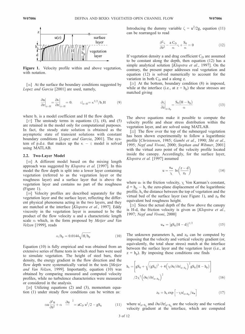
[18] A different model based on the mixing lengthapproach was suggested by Klopstra et al. [1997]. In thismodel the flow depth is split into a lower layer containingvegetation (referred to as the vegetation layer or theroughness layer) and a surface layer that is above thevegetation layer and contains no part of the roughness(Figure 1).[19] Velocity profiles are described separately for the

vegetation layer and the surface layer, reflecting the differ-ent physical phenomena acting in the two layers, and theyare matched at the interface [Klopstra et al., 1997]. Eddyviscosity in the vegetation layer is assumed to be theproduct of the flow velocity u and a characteristic lengthscale a which, in the form proposed by Meijer and VanVelzen [1999], reads

a=hp ¼ 0:0144ffiffiffiffiffiffiffiffiffiffiffiH=hp

qð10Þ

Equation (10) is fully empirical and was obtained from anextensive series of flume tests in which steel bars were usedto simulate vegetation. The height of steel bars, theirdensity, the energy gradient in the flow direction and theflow depth were systematically varied in the tests [Meijerand Van Velzen, 1999]. Importantly, equation (10) wasobtained by comparing measured and computed velocityprofiles, while no turbulence characteristics were measuredor considered in the analysis.[20] Utilizing equations (2) and (3), momentum equa-

tion (1) under steady flow conditions can be written as:

au@2u

@z2þ a

@u 2

¼ aCD u2=2� gS0 ð11Þ

Introducing the dummy variable z = u2/2g, equation (11)can be rearranged to read

@2V@z2

� a CD

aVþ S0

a¼ 0 ð12Þ

If vegetation density a and drag coefficient CD are assumedto be constant along the depth, then equation (12) has asimple analytical solution [Klopstra et al., 1997]. On thecontrary, the present paper addresses real vegetation andequation (12) is solved numerically to account for thevariation in both CD and a along z.[21] At the bottom, boundary condition (8) is imposed,

while at the interface (i.e., at z = hp) the shear stresses arematched giving

@V@z

��z¼hp

¼S0 H� hp �

að13Þ

The above equations make it possible to compute thevelocity profile and shear stress distribution within thevegetation layer, and are solved using MATLAB.[22] The flow over the top of the submerged vegetation

has been shown experimentally to follow a logarithmicprofile [Christensen, 1985; Gambi et al., 1990; Shi et al.,1995; Nepf and Vivoni, 2000; Stephan and Wibmer, 2001]with the virtual zero point of the velocity profile locatedinside the canopy. Accordingly, for the surface layer,Klopstra et al. [1997] assumed

u ¼u*c

lnz� d

z0

� �ð14Þ

where u* is the friction velocity, c Von Karman’s constant,d = hp � hs the zero-plane displacement of the logarithmicprofile, hs the distance between the top of vegetation and thevirtual bed of the surface layer (see Figure 1), and z0 theequivalent bed roughness height.[23] Since the actual depth of the flow above the canopy

is H-d, the friction velocity is given as [Klopstra et al.,1997; Nepf and Vivoni, 2000]

u* ¼ gS0 H� dð Þ½ 1=2 ð15Þ

The unknown parameters hs and z0 can be computed byimposing that the velocity and vertical velocity gradient (or,equivalently, the total shear stress) match at the interfacebetween the surface layer and the vegetation layer (i.e., atz = hp). By imposing these conditions one finds

hs ¼ gS0 þffiffiffiffiffiffiffiffiffiffiffiffiffiffiffiffiffiffiffiffiffiffiffiffiffiffiffiffiffiffiffiffiffiffiffiffiffiffiffiffiffiffiffiffiffiffiffiffiffiffiffiffiffiffiffiffiffiffiffiffiffiffiffiffiffiffiffiffiffiffiffiffiffiffiffiffiffiffiffigS0ð Þ2 þ 4 c@u=@zjz¼hp

� 2gS0 H� hp �r" #

=2c2 @u=@zjz¼hp

� 2ð16Þ

z0 ¼ hs exp �cujz¼hp=u*

h ið17Þ

where ujz=hp and @u/@zjz=hp are the velocity and the verticalvelocity gradient at the interface, which are computed

Figure 1. Velocity profile within and above vegetation,with notation.

W07006 DEFINA AND BIXIO: VEGETATED OPEN CHANNEL FLOW

3 of 12

W07006

using the velocity profile determined for the vegetationlayer.[24] Equations (14) to (17) fully define the velocity

profile within the surface layer. Moreover, it can be shownthat the eddy viscosity and shear stress distributions aregiven by

nT ¼ cffiffiffiffiffiffiffigS0

pH� zð Þ z� dð Þ=

ffiffiffiffiffiffiffiffiffiffiffiffiffiffiffiffiH� dð Þ

pð18Þ

t ¼ r g S0 H� zð Þ ð19Þ

It is clear that the mixing length approach used to computethe eddy viscosity in the two-layer model only provideslimited information on the turbulence structure within andabove the canopy. To overcome this limitation, the two-layermodel was improved by adding an equation expressing thebudget of turbulent kinetic energy. From equation (6) wehave e = Cmk

2/nT, which is used to remove the dissipationrate e in equation (4). The latter can thus be written as

@k@t

¼ @

@z

nTsk

þ n� �

@ k@z

� �þ nT

@u

@z

� �2

� Cmk2=nT þ Cfk ufD

ð20Þ

The above equation is solved with the same boundaryconditions used in the k � e model, i.e., k = 0 at the bottomand @k/@z = 0 at the free surface.[25] It is worth pointing out that when a and CD are

considered constant, equation (11) has the following ana-lytical solution

u ¼

ffiffiffiffiffiffiffiffiffiffiffiffiffiffiffiffiffiffiffiffiffiffiffiffiffiffiffiffiffiffiffiffiffiffiffiffiffiffiffiffiffiffiffiffiffiffiffiffiffiffiffiffiffiffiffiffiffiffiffiffiffiffiffiffiffiffiffiffiffiffiffiffiffiffiffiffiffiffiffiffiffiffiffiffi2gS0

b a=hp � H

hp� 1

� � sinh b z=hp

� h icosh bð Þ þ 1

b

8<:

9=;

vuuut ð21Þ

where

b ¼ hpffiffiffiffiffiffiffiffiffiffiffiffiffiffiaCD=a

p¼

ffiffiffiffiffiffiffiffiffiffiffiffiffiffiffiffiffiffiffiffiffiCD

ahp

a=hp �

sð22Þ

Moreover, from equations (3) and (10) we have

t ¼ tmax

cosh b z=hp

� h icosh bð Þ tmax ¼ tjz¼hp

¼ rgS0 H� hp �

ð23Þ

3. Numerical Simulations

[26] The k � e and two-layer models were compared withexperimental data reported in the literature. These data werefrom laboratory experiments where vegetation was simulatedusing simple rigid cylinders [Lopez and Garcia, 2001;Shimizu and Tsujimoto, 1994; Meijer and Van Velzen,1999], plastic plants [Nepf and Vivoni, 1999, 2000], and realvegetation [Shi et al., 1995; Meijer and Van Velzen, 1999].[27] The experimental data are summarized in Table 1.

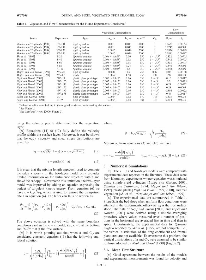
Slope S0 is the bed slope when uniform flow conditions wereattained in the experiments, otherwise S0 is the free surfaceslope. The data of Nepf and Vivoni [2000] and Lopez andGarcia [2001] were derived using a double averagingprocedure where values measured over a number of posi-tions in the horizontal are averaged first in time and then inspace. Unfortunately, the experimental data for Spartinaanglica reported by Shi et al. [1995] are not complete, i.e.,the vertical distribution of the drag coefficient and frontalplant area are not available. To overcome this problem, thevertical distributions of a and CD were assumed to be similarto those adopted by Nepf and Vivoni [1999] (Figure 2).

3.1. Mean Flow Structure

[28] Good agreement between the results of the modelsand experimental measurements was found for velocity and

Table 1. Vegetation and Flow Characteristics for the Flume Experiments Considereda

Source Experiment

Vegetation CharacteristicsFlow

Characteristics

Type Az, m hp, m m, m�2 CD H, m S0

Shimizu and Tsujimoto [1994] ST-R31 rigid cylinders 0.001 0.041 10000 1 0.0631 0.00164Shimizu and Tsujimoto [1994] ST-R32 rigid cylinders 0.001 0.041 10000 1 0.0747 0.0008Shimizu and Tsujimoto [1994] ST-A31 rigid cylinders 0.0015 0.046 2500 1 0.0936 0.00089Shimizu and Tsujimoto [1994] ST-A71 rigid cylinders 0.0015 0.046 2500 1 0.0895 0.00087Shi et al. [1995] S-20 Spartina anglica 0.004 � 0.028b 0.06 350 1 � 2.5b 0.332 0.00003Shi et al. [1995] S-40 Spartina anglica 0.004 � 0.028b 0.12 350 1 � 2.5b 0.342 0.00003Shi et al. [1995] S-60 Spartina anglica 0.004 � 0.028b 0.18 350 1 � 2.5b 0.338 0.00007Shi et al. [1995] S-80 Spartina anglica 0.004 � 0.028b 0.24 350 1 � 2.5b 0.346 0.0006Shi et al. [1995] S-100 Spartina anglica 0.004 � 0.028b 0.3 350 1 � 2.5b 0.348 0.0006Meijer and van Velzen [1999] MV-22 rigid cylinders 0.008 0.9 256 0.87 2.08 0.00188Meijer and van Velzen [1999] MV-R6 reeds 0.0057 1.58 256 1.8 1.99 0.0019Nepf and Vivoni [2000] NV-1.0 plastic plant prototype 0.005 � 0.017c 0.16 330 1 � 3c 0.16 0.00017Nepf and Vivoni [2000] NV-1.25 plastic plant prototype 0.005 � 0.017c 0.16 330 1 � 3c 0.2 0.00025Nepf and Vivoni [2000] NV-1.50 plastic plant prototype 0.005 � 0.017c 0.16 330 1 � 3c 0.24 0.00022Nepf and Vivoni [2000] NV-1.75 plastic plant prototype 0.005 � 0.017c 0.16 330 1 � 3c 0.28 0.0005Nepf and Vivoni [2000] NV-1.90 plastic plant prototype 0.005 � 0.017c 0.16 330 1 � 3c 0.304 0.00022Nepf and Vivoni [2000] NV-2.75 plastic plant prototype 0.005 � 0.017c 0.16 330 1 � 3c 0.44 0.00017Lopez and Garcia [2001] LG-1 rigid cylinders 0.0064 0.12 170 1.13 0.335 0.0036Lopez and Garcia [2001] LG-9 rigid cylinders 0.0064 0.12 384 1.13 0.214 0.0036

aValues in italics were lacking in the original works and estimated by the authors.bSee Figure 2.cSee Nepf and Vivoni [2000, Figure 3].

4 of 12


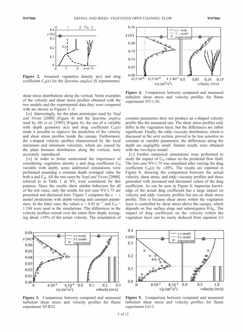
shear stress distributions along the vertical. Some examplesof the velocity and shear stress profiles obtained with thetwo models and the experimental data they were comparedwith are shown in Figures 3–6.[29] Interestingly, for the plant prototypes used by Nepf

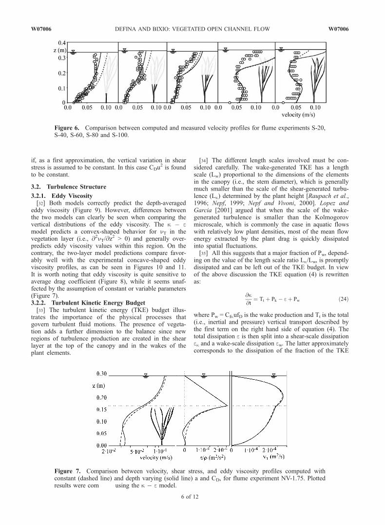
and Vivoni [2000] (Figure 4) and the Spartina anglicaused by Shi et al. [1995] (Figure 6), the use of a variablewith depth geometry a(z) and drag coefficient CD(z)made it possible to improve the prediction of the velocityand shear stress profiles inside the canopy. Furthermore,the s-shaped velocity profiles characterized by the localmaximum and minimum velocities, which are caused bythe plant biomass distribution along the vertical, wereaccurately reproduced.[30] In order to better understand the importance of

considering vegetation density a and drag coefficient CD

variable with depth, some additional simulations wereperformed assuming a constant depth averaged value forboth a and CD. All the test cases by Nepf and Vivoni [2000],referred to in Table 1 as NV, were considered for thispurpose. Since the results show similar behaviors for allof the test cases, only the results for test case NV-1.75 arepresented and discussed here. Figure 7 compares the k � emodel predictions with depth-varying and constant param-eters. In the latter case, the values a = 4.45 m�1 and CD =1.194 were used in the simulations. The differences in thevelocity profiles extend over the entire flow depth, averag-ing about ±10% of the actual velocity. The assumption of

constant parameters does not produce an s-shaped velocityprofile like the measured one. The shear stress profiles onlydiffer in the vegetation layer, but the differences are rathersignificant. Finally, the eddy viscosity distribution, which isdiscussed in the next section, proved to be less sensitive toconstant or variable parameters; the differences along thedepth are negligibly small. Similar results were obtainedwith the two-layer model.[31] Further numerical simulations were performed to

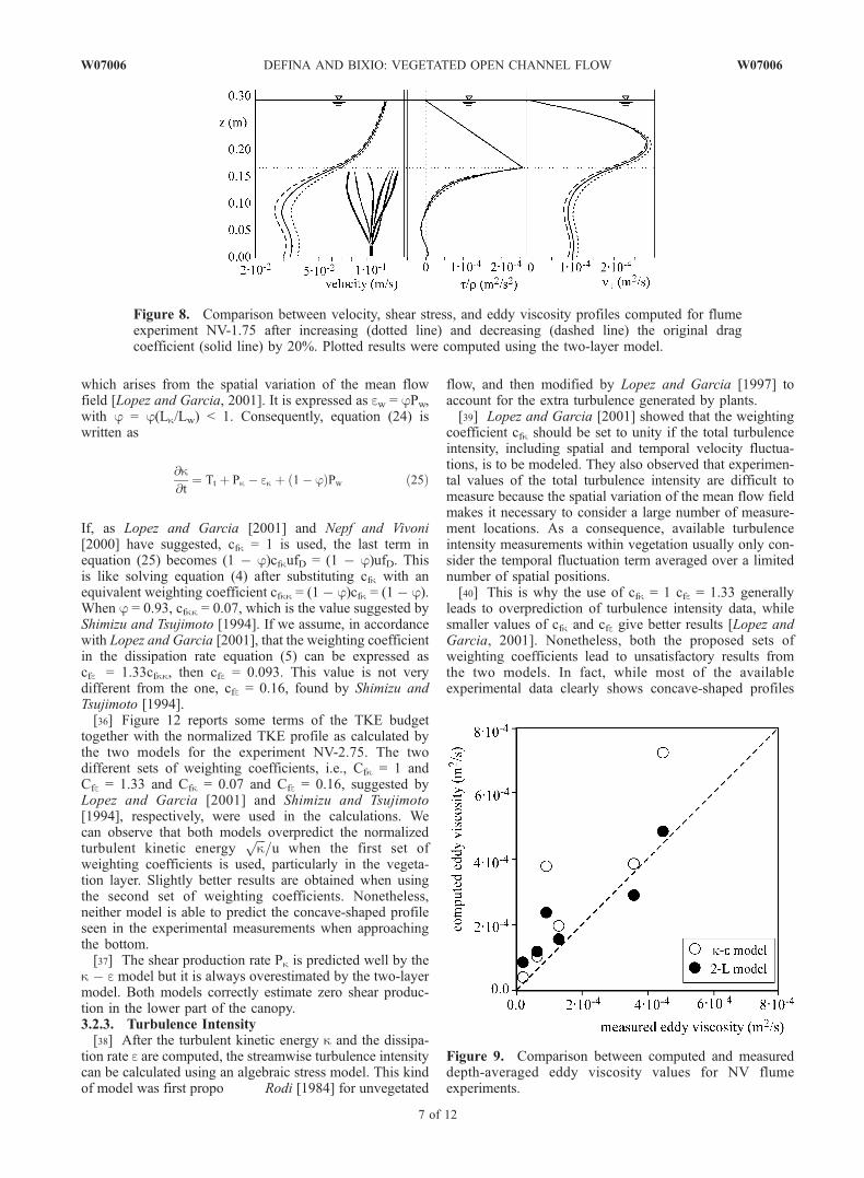
study the impact of CD values on the predicted flow field.The test case NV-1.75 was simulated after varying the dragcoefficient CD(z) by ±20%. The results are reported inFigure 8, showing the comparison between the actualvelocity, shear stress, and eddy viscosity profiles and thosegenerated with increased and decreased values of the dragcoefficient. As can be seen in Figure 8, imprecise knowl-edge of the actual drag coefficient has a large impact onvelocity and eddy viscosity profiles but not on shear stressprofile. This is because shear stress within the vegetationlayer is controlled by shear stress above the canopy, whichdepends on free surface slope and submergence H-hp. Theimpact of drag coefficient on the velocity within thevegetation layer can be easily deduced from equation (1)

Figure 3. Comparison between computed and measuredturbulent shear stress and velocity profiles for flumeexperiment ST-R32.

Figure 2. Assumed vegetation density a(z) and dragcoefficient CD(z) for the Spartina anglica (S experiments).

Figure 4. Comparison between computed and measuredturbulent shear stress and velocity profiles for flumeexperiment NV-1.50.

Figure 5. Comparison between computed and measuredturbulent shear stress and velocity profiles for flumeexperiment LG-1.


5 of 12

W07006

if, as a first approximation, the vertical variation in shearstress is assumed to be constant. In this case CDu

2 is foundto be constant.

3.2. Turbulence Structure

3.2.1. Eddy Viscosity[32] Both models correctly predict the depth-averaged

eddy viscosity (Figure 9). However, differences betweenthe two models can clearly be seen when comparing thevertical distributions of the eddy viscosity. The k � emodel predicts a convex-shaped behavior for nT in thevegetation layer (i.e., @2nT/@z

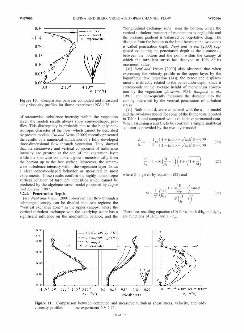
2 > 0) and generally over-predicts eddy viscosity values within this region. On thecontrary, the two-layer model predictions compare favor-ably well with the experimental concave-shaped eddyviscosity profiles, as can be seen in Figures 10 and 11.It is worth noting that eddy viscosity is quite sensitive toaverage drag coefficient (Figure 8), while it seems unaf-fected by the assumption of constant or variable parameters(Figure 7).3.2.2. Turbulent Kinetic Energy Budget[33] The turbulent kinetic energy (TKE) budget illus-

trates the importance of the physical processes thatgovern turbulent fluid motions. The presence of vegeta-tion adds a further dimension to the balance since newregions of turbulence production are created in the shearlayer at the top of the canopy and in the wakes of theplant elements.

[34] The different length scales involved must be con-sidered carefully. The wake-generated TKE has a lengthscale (Lw) proportional to the dimensions of the elementsin the canopy (i.e., the stem diameter), which is generallymuch smaller than the scale of the shear-generated turbu-lence (Lk) determined by the plant height [Raupach et al.,1996; Nepf, 1999; Nepf and Vivoni, 2000]. Lopez andGarcia [2001] argued that when the scale of the wake-generated turbulence is smaller than the Kolmogorovmicroscale, which is commonly the case in aquatic flowswith relatively low plant densities, most of the mean flowenergy extracted by the plant drag is quickly dissipatedinto spatial fluctuations.[35] All this suggests that a major fraction of Pw, depend-

ing on the value of the length scale ratio Lk/Lw, is promptlydissipated and can be left out of the TKE budget. In viewof the above discussion the TKE equation (4) is rewrittenas:

@k@t

¼ Tt þ Pk � eþ Pw ð24Þ

where Pw = CfkufD is the wake production and Tt is the total(i.e., inertial and pressure) vertical transport described bythe first term on the right hand side of equation (4). Thetotal dissipation e is then split into a shear-scale dissipationek and a wake-scale dissipation ew. The latter approximatelycorresponds to the dissipation of the fraction of the TKE

Figure 6. Comparison between computed and measured velocity profiles for flume experiments S-20,S-40, S-60, S-80 and S-100.

Figure 7. Comparison between velocity, shear stress, and eddy viscosity profiles computed withconstant (dashed line) and depth varying (solid line) a and CD, for flume experiment NV-1.75. Plottedresults were com using the k � e model.

6 of 12


which arises from the spatial variation of the mean flowfield [Lopez and Garcia, 2001]. It is expressed as ew = jPw,with j = j(Lk/Lw) < 1. Consequently, equation (24) iswritten as

@k@t

¼ Tt þ Pk � ek þ 1� jð ÞPw ð25Þ

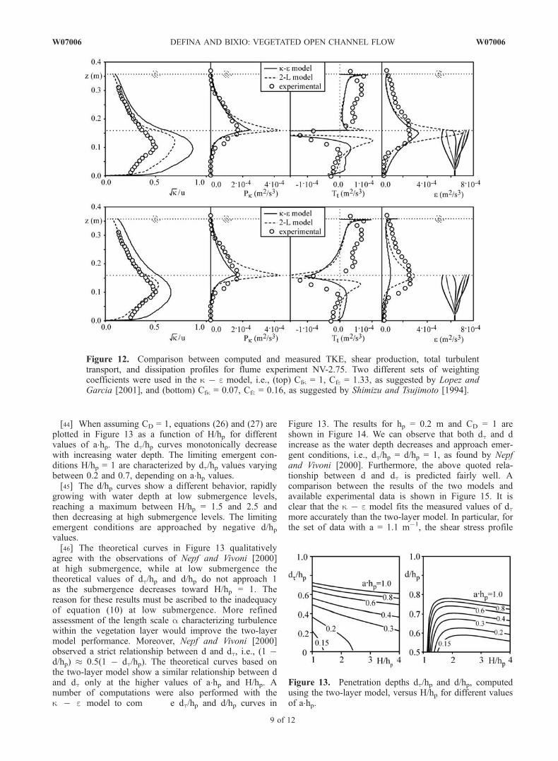
If, as Lopez and Garcia [2001] and Nepf and Vivoni[2000] have suggested, cfk = 1 is used, the last term inequation (25) becomes (1 � j)cfkufD = (1 � j)ufD. Thisis like solving equation (4) after substituting cfk with anequivalent weighting coefficient cfkk = (1 � j)cfk = (1 � j).When j = 0.93, cfkk = 0.07, which is the value suggested byShimizu and Tsujimoto [1994]. If we assume, in accordancewith Lopez and Garcia [2001], that the weighting coefficientin the dissipation rate equation (5) can be expressed ascfe = 1.33cfkk, then cfe = 0.093. This value is not verydifferent from the one, cfe = 0.16, found by Shimizu andTsujimoto [1994].[36] Figure 12 reports some terms of the TKE budget

together with the normalized TKE profile as calculated bythe two models for the experiment NV-2.75. The twodifferent sets of weighting coefficients, i.e., Cfk = 1 andCfe = 1.33 and Cfk = 0.07 and Cfe = 0.16, suggested byLopez and Garcia [2001] and Shimizu and Tsujimoto[1994], respectively, were used in the calculations. Wecan observe that both models overpredict the normalizedturbulent kinetic energy

ffiffiffik

p=u when the first set of

weighting coefficients is used, particularly in the vegeta-tion layer. Slightly better results are obtained when usingthe second set of weighting coefficients. Nonetheless,neither model is able to predict the concave-shaped profileseen in the experimental measurements when approachingthe bottom.[37] The shear production rate Pk is predicted well by the

k � e model but it is always overestimated by the two-layermodel. Both models correctly estimate zero shear produc-tion in the lower part of the canopy.3.2.3. Turbulence Intensity[38] After the turbulent kinetic energy k and the dissipa-

tion rate e are computed, the streamwise turbulence intensitycan be calculated using an algebraic stress model. This kindof model was first propo Rodi [1984] for unvegetated

flow, and then modified by Lopez and Garcia [1997] toaccount for the extra turbulence generated by plants.[39] Lopez and Garcia [2001] showed that the weighting

coefficient cfk should be set to unity if the total turbulenceintensity, including spatial and temporal velocity fluctua-tions, is to be modeled. They also observed that experimen-tal values of the total turbulence intensity are difficult tomeasure because the spatial variation of the mean flow fieldmakes it necessary to consider a large number of measure-ment locations. As a consequence, available turbulenceintensity measurements within vegetation usually only con-sider the temporal fluctuation term averaged over a limitednumber of spatial positions.[40] This is why the use of cfk = 1 cfe = 1.33 generally

leads to overprediction of turbulence intensity data, whilesmaller values of cfk and cfe give better results [Lopez andGarcia, 2001]. Nonetheless, both the proposed sets ofweighting coefficients lead to unsatisfactory results fromthe two models. In fact, while most of the availableexperimental data clearly shows concave-shaped profiles

Figure 8. Comparison between velocity, shear stress, and eddy viscosity profiles computed for flumeexperiment NV-1.75 after increasing (dotted line) and decreasing (dashed line) the original dragcoefficient (solid line) by 20%. Plotted results were computed using the two-layer model.

Figure 9. Comparison between computed and measureddepth-averaged eddy viscosity values for NV flumeexperiments.


7 of 12

W07006

of streamwise turbulence intensity within the vegetationlayer, the models results always show convex-shaped pro-files. This discrepancy is probably due to the highly non-isotropic character of the flow, which cannot be describedby present models. Cui and Neary [2002] recently presentedthe results of a numerical simulation of a fully developedthree-dimensional flow through vegetation. They showedthat the streamwise and vertical component of turbulenceintensity are greatest at the top of the vegetation layerwhile the spanwise component grows monotonically fromthe bottom up to the free surface. Moreover, the stream-wise turbulence intensity within the vegetation layer showsa clear concave-shaped behavior as measured in mostexperiments. These results confirm the highly nonisotropicvertical behavior of turbulent intensities which cannot bepredicted by the algebraic stress model proposed by Lopezand Garcia [1997].3.2.4. Penetration Depth[41] Nepf and Vivoni [2000] observed that flow through a

submerged canopy can be divided into two regions: the‘‘vertical exchange zone’’ in the upper canopy, where thevertical turbulent exchange with the overlying water has asignificant influence on the momentum balance, and the

‘‘longitudinal exchange zone’’ near the bottom, where thevertical turbulent transport of momentum is negligible andthe pressure gradient is balanced by vegetative drag. Thedistance from the bottom to the limit between the two zonesis called penetration depth. Nepf and Vivoni [2000] sug-gested evaluating the penetration depth as the distance dtbetween the bottom and the point within the canopy atwhich the turbulent stress has decayed to 10% of itsmaximum value.[42] Nepf and Vivoni [2000] also observed that when

expressing the velocity profile in the upper layer by thelogarithmic law (equation (14)), the zero-plane displace-ment d is directly related to the penetration depth, since itcorresponds to the average height of momentum absorp-tion by the vegetation [Jackson, 1981; Raupach et al.,1991], and consequently measures the distance into thecanopy interested by the vertical penetration of turbulentstress.[43] Both d and dt were calculated with the k � e model

and the two-layer model for some of the flume tests reportedin Table 1, and compared with available experimental data.When assuming a and CD to be constant, a simple analyticalsolution is provided by the two-layer model:

dt

hp¼ 1� 1

b‘n

1:1þ tanh b�ffiffiffiffiffiffiffiffiffiffiffiffiffiffiffiffiffiffiffiffiffiffiffiffiffiffiffiffitanh2 b� 0:99

p1:1� tanh bþ

ffiffiffiffiffiffiffiffiffiffiffiffiffiffiffiffiffiffiffiffiffiffiffiffiffiffiffiffitanh2 b� 0:99

p ð26Þ

d

hp¼ 1�M

H

hp� 1

� �1þ

ffiffiffiffiffiffiffiffiffiffiffiffiffi1þ 2

M

r !ð27Þ

where b is given by equation (22) and

M ¼ 1

c2

ahp

� � 1þ bH

hp� 1

� �tanh b

b2H

hp� 1

� �3ð28Þ

Therefore, recalling equation (10) for a, both d/hp and dt/hpare functions of H/hp and a � hp.

Figure 10. Comparison between computed and measurededdy viscosity profiles for flume experiment NV-1.75.

Figure 11. Comparison between computed and measured turbulent shear stress, velocity, and eddyviscosity profiles me experiment NV-2.75.

8 of 12


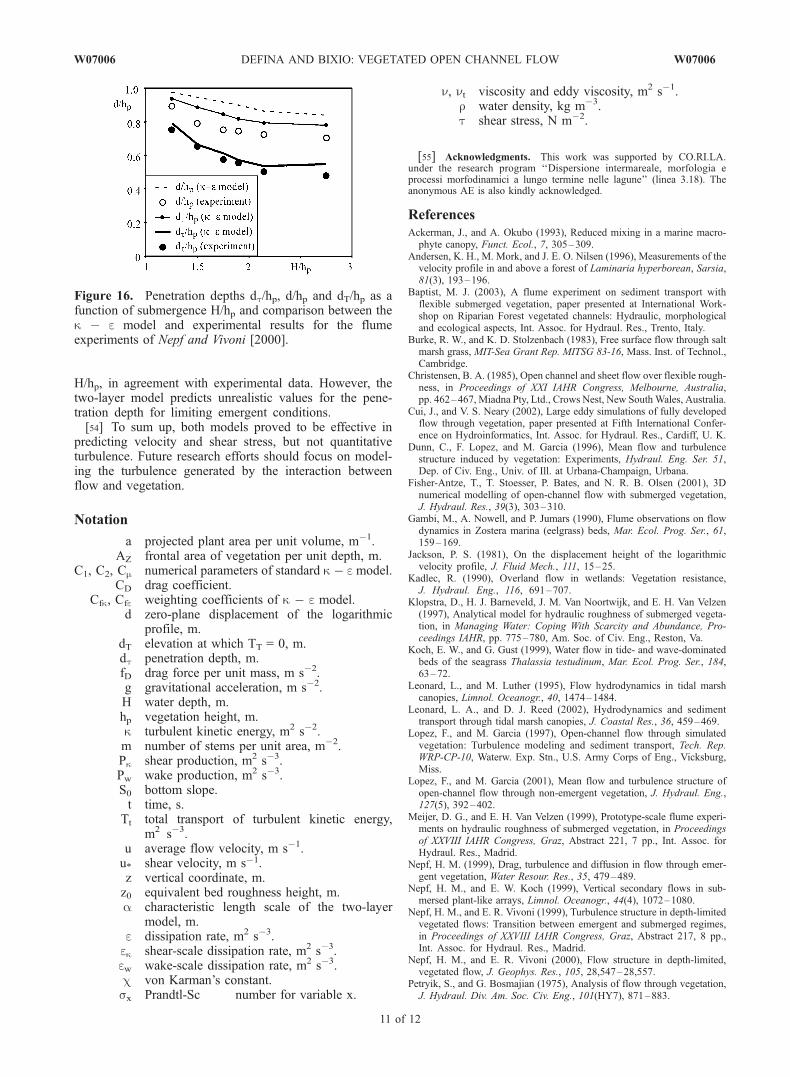
[44] When assuming CD = 1, equations (26) and (27) areplotted in Figure 13 as a function of H/hp for differentvalues of a�hp. The dt/hp curves monotonically decreasewith increasing water depth. The limiting emergent con-ditions H/hp = 1 are characterized by dt/hp values varyingbetween 0.2 and 0.7, depending on a�hp values.[45] The d/hp curves show a different behavior, rapidly

growing with water depth at low submergence levels,reaching a maximum between H/hp = 1.5 and 2.5 andthen decreasing at high submergence levels. The limitingemergent conditions are approached by negative d/hpvalues.[46] The theoretical curves in Figure 13 qualitatively

agree with the observations of Nepf and Vivoni [2000]at high submergence, while at low submergence thetheoretical values of dt/hp and d/hp do not approach 1as the submergence decreases toward H/hp = 1. Thereason for these results must be ascribed to the inadequacyof equation (10) at low submergence. More refinedassessment of the length scale a characterizing turbulencewithin the vegetation layer would improve the two-layermodel performance. Moreover, Nepf and Vivoni [2000]observed a strict relationship between d and dt, i.e., (1 �d/hp) 0.5(1 � dt/hp). The theoretical curves based onthe two-layer model show a similar relationship between dand dt only at the higher values of a�hp and H/hp. Anumber of computations were also performed with thek � e model to com e dt/hp and d/hp curves in

Figure 13. The results for hp = 0.2 m and CD = 1 areshown in Figure 14. We can observe that both dt and dincrease as the water depth decreases and approach emer-gent conditions, i.e., dt/hp = d/hp = 1, as found by Nepfand Vivoni [2000]. Furthermore, the above quoted rela-tionship between d and dt is predicted fairly well. Acomparison between the results of the two models andavailable experimental data is shown in Figure 15. It isclear that the k � e model fits the measured values of dtmore accurately than the two-layer model. In particular, forthe set of data with a = 1.1 m�1, the shear stress profile

Figure 12. Comparison between computed and measured TKE, shear production, total turbulenttransport, and dissipation profiles for flume experiment NV-2.75. Two different sets of weightingcoefficients were used in the k � e model, i.e., (top) Cfk = 1, Cfe = 1.33, as suggested by Lopez andGarcia [2001], and (bottom) Cfk = 0.07, Cfe = 0.16, as suggested by Shimizu and Tsujimoto [1994].

Figure 13. Penetration depths dt/hp and d/hp, computedusing the two-layer model, versus H/hp for different valuesof a�hp.


9 of 12

W07006

within the vegetation layer predicted by the two-layermodel shows values that are always larger than 10% ofthe maximum shear stress (Figure 5). This leads to dt = 0and thus to a predicted vertical exchange zone extendingthrough the whole vegetation layer.[47] Nepf and Vivoni [2000] also argued that penetration

depth should increase as vegetation density a increases.However, as can be seen in Figure 15, the penetration depthis greater in experiments with a = 5.5 m�1 than in those witha = 10 m�1. On the contrary, when the parameter a�hp isused to qualify vegetation density, as suggested by theanalytical solution of the two-layer model, we can see thatthe penetration depth does increase as the vegetation densityincreases (Figure 15).[48] A further definition of the penetration depth can be

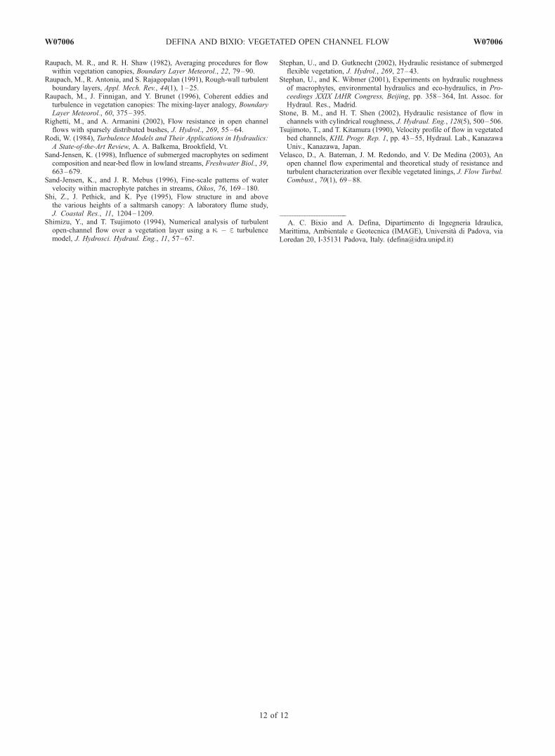
based on the transport term Tt of the turbulent kineticenergy budget equation (24). This term represents the totalvertical transport of turbulent kinetic energy, and is respon-sible for removing energy from the canopy top region andfor redistributing it within the vegetation layer. Sincenegative Tt values in the upper part of the canopy charac-terize the vertical exchange zone, the penetration depths dand dt have been compared with the elevation above thebottom, dT, at which Tt jumps to zero before assuming smallnegative values. Figure 16 compares the results computedwith the k � e model with the experimental data of Nepf

and Vivoni [2000], showing good agreement between dTand d.

4. Conclusions

[49] A number of numerical simulations were performedusing the k � e model and the two-layer model in order totest their ability to predict the flow field in the presence ofrigid vegetation. A comparison between experimental dataand the results of these simulations clearly demonstrates thatboth models can fairly accurately reproduce the verticalprofiles of velocity and shear stress within and abovevegetation. Therefore these models can be used to assessvegetative resistance to flow. Moreover, the results can beeven more accurate when the plant geometry and dragcoefficient variation along the vertical are taken into ac-count. It has also been shown that the values assumed forthe drag coefficient strongly affect the velocity profile buthave a minor impact on shear stress.[50] Eddy viscosity profiles are fairly accurately predicted

by the two-layer model. The k � e model, on the otherhand, does not accurately predict the behavior of eddyviscosity within the vegetation layer. In this layer, the modelpredicts a parabolic profile and generally overestimates theexperimental values.[51] Turbulence characteristics are poorly predicted by

both the models. This is mainly because the models are notable to effectively account for the presence of both the shearand wake turbulence length scales. However, there is alsosome uncertainty in the experimental data because measur-ing flow velocity in the presence of vegetation is quitedifficult given that the spatial variation of the mean flowfield makes it necessary to consider a large number ofmeasurement locations.[52] The penetration depth of turbulent stress inside the

canopy was estimated according to different criteria. Thesewere based on the analysis of vertical profiles of Reynolds’stress, velocity and the total transport of turbulent kineticenergy. The results of the two models confirmed theexperimentally observed trend of dt/hp increasing as vege-tation density increases if the product a�hp is used instead ofa to characterize the vegetation density.[53] Results obtained using the k � e model showed that

penetration depth is a decreasing function of depth ratio

Figure 14. Penetration depths dt/hp and d/hp, computedusing the k � e model, versus H/hp for different values ofa�hp.

Figure 15. Comparison between computed and measured penetration depth dt/hp. Original values ofdrag coefficient and vegetation density were used in the computations. For the NV case the computedpenetration depth used variable CD and a; the value a = 5.5 m�1 reported here is a representativevegetation densit Nepf and Vivoni, 2000, Figure 9].

10 of 12


H/hp, in agreement with experimental data. However, thetwo-layer model predicts unrealistic values for the pene-tration depth for limiting emergent conditions.[54] To sum up, both models proved to be effective in

predicting velocity and shear stress, but not quantitativeturbulence. Future research efforts should focus on model-ing the turbulence generated by the interaction betweenflow and vegetation.

Notation

a projected plant area per unit volume, m�1.AZ frontal area of vegetation per unit depth, m.

C1, C2, Cm numerical parameters of standard k � e model.CD drag coefficient.

Cfk, Cfe weighting coefficients of k � e model.d zero-plane displacement of the logarithmic

profile, m.dT elevation at which TT = 0, m.dt penetration depth, m.fD drag force per unit mass, m s�2.g gravitational acceleration, m s�2.H water depth, m.hp vegetation height, m.k turbulent kinetic energy, m2 s�2.m number of stems per unit area, m�2.Pk shear production, m2 s�3.Pw wake production, m2 s�3.S0 bottom slope.t time, s.

Tt total transport of turbulent kinetic energy,m2 s�3.

u average flow velocity, m s�1.u* shear velocity, m s�1.z vertical coordinate, m.z0 equivalent bed roughness height, m.a characteristic length scale of the two-layer

model, m.e dissipation rate, m2 s�3.ek shear-scale dissipation rate, m2 s�3.ew wake-scale dissipation rate, m2 s�3.c von Karman’s constant.sx Prandtl-Sc number for variable x.

n, nt viscosity and eddy viscosity, m2 s�1.r water density, kg m�3.t shear stress, N m�2.

[55] Acknowledgments. This work was supported by CO.RI.LA.under the research program ‘‘Dispersione intermareale, morfologia eprocessi morfodinamici a lungo termine nelle lagune’’ (linea 3.18). Theanonymous AE is also kindly acknowledged.

ReferencesAckerman, J., and A. Okubo (1993), Reduced mixing in a marine macro-phyte canopy, Funct. Ecol., 7, 305–309.

Andersen, K. H., M. Mork, and J. E. O. Nilsen (1996), Measurements of thevelocity profile in and above a forest of Laminaria hyperborean, Sarsia,81(3), 193–196.

Baptist, M. J. (2003), A flume experiment on sediment transport withflexible submerged vegetation, paper presented at International Work-shop on Riparian Forest vegetated channels: Hydraulic, morphologicaland ecological aspects, Int. Assoc. for Hydraul. Res., Trento, Italy.

Burke, R. W., and K. D. Stolzenbach (1983), Free surface flow through saltmarsh grass, MIT-Sea Grant Rep. MITSG 83-16, Mass. Inst. of Technol.,Cambridge.

Christensen, B. A. (1985), Open channel and sheet flow over flexible rough-ness, in Proceedings of XXI IAHR Congress, Melbourne, Australia,pp. 462–467, Miadna Pty, Ltd., Crows Nest, New SouthWales, Australia.

Cui, J., and V. S. Neary (2002), Large eddy simulations of fully developedflow through vegetation, paper presented at Fifth International Confer-ence on Hydroinformatics, Int. Assoc. for Hydraul. Res., Cardiff, U. K.

Dunn, C., F. Lopez, and M. Garcia (1996), Mean flow and turbulencestructure induced by vegetation: Experiments, Hydraul. Eng. Ser. 51,Dep. of Civ. Eng., Univ. of Ill. at Urbana-Champaign, Urbana.

Fisher-Antze, T., T. Stoesser, P. Bates, and N. R. B. Olsen (2001), 3Dnumerical modelling of open-channel flow with submerged vegetation,J. Hydraul. Res., 39(3), 303–310.

Gambi, M., A. Nowell, and P. Jumars (1990), Flume observations on flowdynamics in Zostera marina (eelgrass) beds, Mar. Ecol. Prog. Ser., 61,159–169.

Jackson, P. S. (1981), On the displacement height of the logarithmicvelocity profile, J. Fluid Mech., 111, 15–25.

Kadlec, R. (1990), Overland flow in wetlands: Vegetation resistance,J. Hydraul. Eng., 116, 691–707.

Klopstra, D., H. J. Barneveld, J. M. Van Noortwijk, and E. H. Van Velzen(1997), Analytical model for hydraulic roughness of submerged vegeta-tion, in Managing Water: Coping With Scarcity and Abundance, Pro-ceedings IAHR, pp. 775–780, Am. Soc. of Civ. Eng., Reston, Va.

Koch, E. W., and G. Gust (1999), Water flow in tide- and wave-dominatedbeds of the seagrass Thalassia testudinum, Mar. Ecol. Prog. Ser., 184,63–72.

Leonard, L., and M. Luther (1995), Flow hydrodynamics in tidal marshcanopies, Limnol. Oceanogr., 40, 1474–1484.

Leonard, L. A., and D. J. Reed (2002), Hydrodynamics and sedimenttransport through tidal marsh canopies, J. Coastal Res., 36, 459–469.

Lopez, F., and M. Garcia (1997), Open-channel flow through simulatedvegetation: Turbulence modeling and sediment transport, Tech. Rep.WRP-CP-10, Waterw. Exp. Stn., U.S. Army Corps of Eng., Vicksburg,Miss.

Lopez, F., and M. Garcia (2001), Mean flow and turbulence structure ofopen-channel flow through non-emergent vegetation, J. Hydraul. Eng.,127(5), 392–402.

Meijer, D. G., and E. H. Van Velzen (1999), Prototype-scale flume experi-ments on hydraulic roughness of submerged vegetation, in Proceedingsof XXVIII IAHR Congress, Graz, Abstract 221, 7 pp., Int. Assoc. forHydraul. Res., Madrid.

Nepf, H. M. (1999), Drag, turbulence and diffusion in flow through emer-gent vegetation, Water Resour. Res., 35, 479–489.

Nepf, H. M., and E. W. Koch (1999), Vertical secondary flows in sub-mersed plant-like arrays, Limnol. Oceanogr., 44(4), 1072–1080.

Nepf, H. M., and E. R. Vivoni (1999), Turbulence structure in depth-limitedvegetated flows: Transition between emergent and submerged regimes,in Proceedings of XXVIII IAHR Congress, Graz, Abstract 217, 8 pp.,Int. Assoc. for Hydraul. Res., Madrid.

Nepf, H. M., and E. R. Vivoni (2000), Flow structure in depth-limited,vegetated flow, J. Geophys. Res., 105, 28,547–28,557.

Petryik, S., and G. Bosmajian (1975), Analysis of flow through vegetation,J. Hydraul. Div. Am. Soc. Civ. Eng., 101(HY7), 871–883.

Figure 16. Penetration depths dt/hp, d/hp and dT/hp as afunction of submergence H/hp and comparison between thek � e model and experimental results for the flumeexperiments of Nepf and Vivoni [2000].


11 of 12

W07006

Raupach, M. R., and R. H. Shaw (1982), Averaging procedures for flowwithin vegetation canopies, Boundary Layer Meteorol., 22, 79–90.

Raupach, M., R. Antonia, and S. Rajagopalan (1991), Rough-wall turbulentboundary layers, Appl. Mech. Rev., 44(1), 1–25.

Raupach, M., J. Finnigan, and Y. Brunet (1996), Coherent eddies andturbulence in vegetation canopies: The mixing-layer analogy, BoundaryLayer Meteorol., 60, 375–395.

Righetti, M., and A. Armanini (2002), Flow resistance in open channelflows with sparsely distributed bushes, J. Hydrol., 269, 55–64.

Rodi, W. (1984), Turbulence Models and Their Applications in Hydraulics:A State-of-the-Art Review, A. A. Balkema, Brookfield, Vt.

Sand-Jensen, K. (1998), Influence of submerged macrophytes on sedimentcomposition and near-bed flow in lowland streams, Freshwater Biol., 39,663–679.

Sand-Jensen, K., and J. R. Mebus (1996), Fine-scale patterns of watervelocity within macrophyte patches in streams, Oikos, 76, 169–180.

Shi, Z., J. Pethick, and K. Pye (1995), Flow structure in and abovethe various heights of a saltmarsh canopy: A laboratory flume study,J. Coastal Res., 11, 1204–1209.

Shimizu, Y., and T. Tsujimoto (1994), Numerical analysis of turbulentopen-channel flow over a vegetation layer using a k � e turbulencemodel, J. Hydrosci. Hydraul. Eng., 11, 57–67.

Stephan, U., and D. Gutknecht (2002), Hydraulic resistance of submergedflexible vegetation, J. Hydrol., 269, 27–43.

Stephan, U., and K. Wibmer (2001), Experiments on hydraulic roughnessof macrophytes, environmental hydraulics and eco-hydraulics, in Pro-ceedings XXIX IAHR Congress, Beijing, pp. 358–364, Int. Assoc. forHydraul. Res., Madrid.

Stone, B. M., and H. T. Shen (2002), Hydraulic resistance of flow inchannels with cylindrical roughness, J. Hydraul. Eng., 128(5), 500–506.

Tsujimoto, T., and T. Kitamura (1990), Velocity profile of flow in vegetatedbed channels, KHL Progr. Rep. 1, pp. 43–55, Hydraul. Lab., KanazawaUniv., Kanazawa, Japan.

Velasco, D., A. Bateman, J. M. Redondo, and V. De Medina (2003), Anopen channel flow experimental and theoretical study of resistance andturbulent characterization over flexible vegetated linings, J. Flow Turbul.Combust., 70(1), 69–88.

��A. C. Bixio and A. Defina, Dipartimento di Ingegneria Idraulica,

Marittima, Ambientale e Geotecnica (IMAGE), Universita di Padova, viaLoredan 20, I-35131 Padova, Italy. ([email protected])

12 of 12


Documents

Mean flow and turbulence in vegetated open channel flo · · 2012-03-12Mean flow and turbulence in vegetated open channel flow Andrea Defina and Anna Chiara Bixio Dipartimento di