Embed Size (px)
Citation preview
Measure Theory
V. Liskevich
1998
1 Introduction
We always denote by X our universe, i.e. all the sets we shall consider are subsets of X.
Recall some standard notation. 2X everywhere denotes the set of all subsets of a givenset X. If A ∩ B = ∅ then we often write A t B rather than A ∪ B, to underline thedisjointness. The complement (in X) of a set A is denoted by Ac. By A4B the symmetricdifference of A and B is denoted, i.e. A4B = (A \B) ∪ (B \A). Letters i, j, k alwaysdenote positive integers. The sign � is used for restriction of a function (operator etc.) toa subset (subspace).
1.1 The Riemann integral
Recall how to construct the Riemannian integral. Let f : [a, b] → R. Consider a partitionπ of [a, b]:
a = x0 < x1 < x2 < . . . < xn−1 < xn = b
and set ∆xk = xk+1 − xk, |π| = max{∆xk : k = 0, 1, . . . , n − 1}, mk = inf{f(x) : x ∈[xk, xk+1]}, Mk = sup{f(x) : x ∈ [xk, xk+1]}. Define the upper and lower Riemann—Darboux sums
s(f, π) =n−1∑k=0
mk∆xk, s(f, π) =n−1∑k=0
Mk∆xk.
One can show (the Darboux theorem) that the following limits exist
lim|π|→0
s(f, π) = supπ
s(f, π) =
∫ b
a
fdx
lim|π|→0
s(f, π) = infπ
s(f, π) =
∫ b
a
fdx.
1
Clearly,
s(f, π) ≤∫ b
a
fdx ≤∫ b
a
fdx ≤ s(f, π)
for any partition π.
The function f is said to be Riemann integrable on [a, b] if the upper and lower integralsare equal. The common value is called Riemann integral of f on [a, b].
The functions cannot have a large set of points of discontinuity. More presicely thiswill be stated further.
1.2 The Lebesgue integral
It allows to integrate functions from a much more general class. First, consider a veryuseful example. For f, g ∈ C[a, b], two continuous functions on the segment [a, b] = {x ∈R : a 6 x 6 b} put
ρ1(f, g) = maxa6x6b
|f(x)− g(x)|,
ρ2(f, g) =
∫ b
a
|f(x)− g(x)|dx.
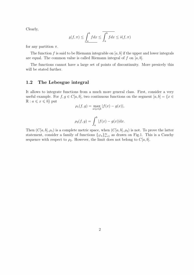
Then (C[a, b], ρ1) is a complete metric space, when (C[a, b], ρ2) is not. To prove the latterstatement, consider a family of functions {ϕn}∞n=1 as drawn on Fig.1. This is a Cauchysequence with respect to ρ2. However, the limit does not belong to C[a, b].
2
-
6
���������� L
LLLLLLLLL
−12
+ 1n
12− 1
n−1
212
Figure 1: The function ϕn.
2 Systems of Sets
Definition 2.1 A ring of sets is a non-empty subset in 2X which is closed with respectto the operations ∪ and \.
Proposition. Let K be a ring of sets. Then ∅ ∈ K.
Proof. Since K 6= ∅, there exists A ∈ K. Since K contains the difference of every twoits elements, one has A \ A = ∅ ∈ K. �
Examples.
1. The two extreme cases are K = {∅} and K = 2X .
2. Let X = R and denote by K all finite unions of semi-segments [a, b).
Definition 2.2 A semi-ring is a collection of sets P ⊂ 2X with the following properties:
1. If A, B ∈ P then A ∩B ∈ P;
3
2. For every A, B ∈ P there exists a finite disjoint collection (Cj) j = 1, 2, . . . , n ofsets (i.e. Ci ∩ Cj = ∅ if i 6= j) such that
A \B =n⊔
j=1
Cj.
Example. Let X = R, then the set of all semi-segments, [a, b), forms a semi-ring.
Definition 2.3 An algebra (of sets) is a ring of sets containing X ∈ 2X .
Examples.
1. {∅, X} and 2X are the two extreme cases (note that they are different from thecorresponding cases for rings of sets).
2. Let X = [a, b) be a fixed interval on R. Then the system of finite unions of subin-tervals [α, β) ⊂ [a, b) forms an algebra.
3. The system of all bounded subsets of the real axis is a ring (not an algebra).
Remark. A is algebra if (i) A, B ∈ A =⇒ A ∪B ∈ A, (ii) A ∈ A =⇒ Ac ∈ A.
Indeed, 1) A ∩B = (Ac ∪Bc)c; 2) A \B = A ∩Bc.
Definition 2.4 A σ-ring (a σ-algebra) is a ring (an algebra) of sets which is closed withrespect to all countable unions.
Definition 2.5 A ring (an algebra, a σ-algebra) of sets, K(U) generated by a collectionof sets U ⊂ 2X is the minimal ring (algebra, σ-algebra) of sets containing U.
In other words, it is the intersection of all rings (algebras, σ-algebras) of sets containingU.
4
3 Measures
Let X be a set, A an algebra on X.
Definition 3.1 A function µ: A −→ R+ ∪ {∞} is called a measure if
1. µ(A) > 0 for any A ∈ A and µ(∅) = 0;
2. if (Ai)i>1 is a disjoint family of sets in A ( Ai ∩ Aj = ∅ for any i 6= j) such that⊔∞i=1 Ai ∈ A, then
µ(∞⊔i=1
Ai) =∞∑i=1
µ(Ai).
The latter important property, is called countable additivity or σ-additivity of the measureµ.
Let us state now some elementary properties of a measure. Below till the end of thissection A is an algebra of sets and µ is a measure on it.
1. (Monotonicity of µ) If A, B ∈ A and B ⊂ A then µ(B) 6 µ(A).
Proof. A = (A \B) tB implies that
µ(A) = µ(A \B) + µ(B).
Since µ(A \B) ≥ 0 it follows that µ(A) ≥ µ(B).
2. (Subtractivity of µ). If A, B ∈ A and B ⊂ A and µ(B) < ∞ then µ(A \ B) =µ(A)− µ(B).
Proof. In 1) we proved that
µ(A) = µ(A \B) + µ(B).
If µ(B) < ∞ thenµ(A)− µ(B) = µ(A \B).
3. If A, B ∈ A and µ(A ∩B) < ∞ then µ(A ∪B) = µ(A) + µ(B)− µ(A ∩B).
Proof. A ∩B ⊂ A, A ∩B ⊂ B, therefore
A ∪B = (A \ (A ∩B)) tB.
Since µ(A ∩B) < ∞, one has
µ(A ∪B) = (µ(A)− µ(A ∩B)) + µ(B).
5
4. (Semi-additivity of µ). If (Ai)i≥1 ⊂ A such that⋃∞
i=1 Ai ∈ A then
µ(∞⋃i=1
Ai) 6∞∑i=1
µ(Ai).
Proof. First let us proove that
µ(n⋃
i=1
Ai) 6n∑
i=1
µ(Ai).
Note that the family of sets
B1 = A1
B2 = A2 \ A1
B3 = A3 \ (A1 ∪ A2)
. . .
Bn = An \n−1⋃i=1
Ai
is disjoint and⊔n
i=1 Bi =⋃n
i=1 Ai. Moreover, since Bi ⊂ Ai, we see that µ(Bi) ≤µ(Ai). Then
µ(n⋃
i=1
Ai) = µ(n⊔
i=1
Bi) =n∑
i=1
µ(Bi) ≤n∑
i=1
µ(Ai).
Now we can repeat the argument for the infinite family using σ-additivity of themeasure.
3.1 Continuity of a measure
Theorem 3.1 Let A be an algebra, (Ai)i≥1 ⊂ A a monotonically increasing sequence ofsets (Ai ⊂ Ai+1) such that
⋃i≥1 ∈ A. Then
µ(∞⋃i=1
Ai) = limn→∞
µ(An).
Proof. 1). If for some n0 µ(An0) = +∞ then µ(An) = +∞∀n ≥ n0 and µ(⋃∞
i=1 Ai) = +∞.
2). Let now µ(Ai) < ∞ ∀i ≥ 1.
6
Then
µ(∞⋃i=1
Ai) = µ(A1 t (A2 \ A1) t . . . t (An \ An−1) t . . .)
= µ(A1) +∞∑
k=2
µ(Ak \ Ak−1)
= µ(A1) + limn→∞
n∑k=2
(µ(Ak)− µ(Ak−1)) = limn→∞
µ(An).
3.2 Outer measure
Let a be an algebra of subsets of X and µ a measure on it. Our purpose now is to extendµ to as many elements of 2X as possible.
An arbitrary set A ⊂ X can be always covered by sets from A, i.e. one can always findE1, E2, . . . ∈ A such that
⋃∞i=1 Ei ⊃ A. For instance, E1 = X, E2 = E3 = . . . = ∅.
Definition 3.2 For A ⊂ X its outer measure is defined by
µ∗(A) = inf∞∑i=1
µ(Ei)
where the infimum is taken over all A-coverings of the set A, i.e. all collections (Ei), Ei ∈A with
⋃i Ei ⊃ A.
Remark. The outer measure always exists since µ(A) > 0 for every A ∈ A.
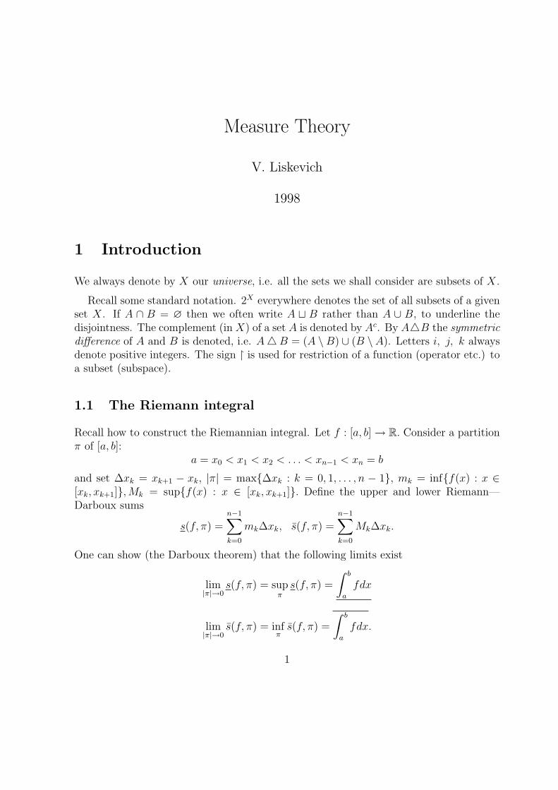
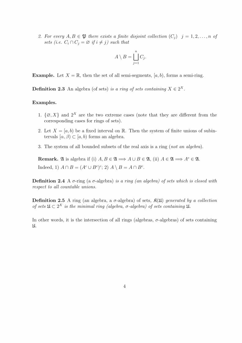
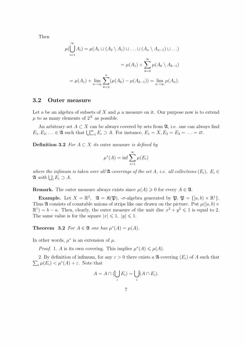
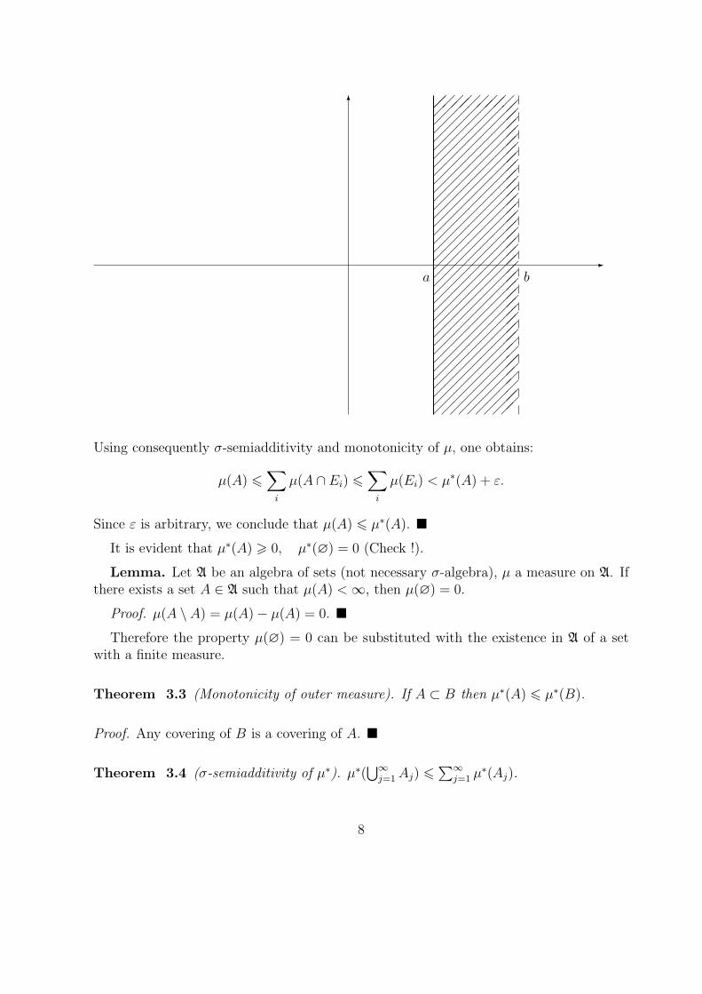
Example. Let X = R2, A = K(P), -σ-algebra generated by P, P = {[a, b) × R1}.Thus A consists of countable unions of strips like one drawn on the picture. Put µ([a, b)×R1) = b − a. Then, clearly, the outer measure of the unit disc x2 + y2 6 1 is equal to 2.The same value is for the square |x| 6 1, |y| 6 1.
Theorem 3.2 For A ∈ A one has µ∗(A) = µ(A).
In other words, µ∗ is an extension of µ.
Proof. 1. A is its own covering. This implies µ∗(A) 6 µ(A).
2. By definition of infimum, for any ε > 0 there exists a A-covering (Ei) of A such that∑i µ(Ei) < µ∗(A) + ε. Note that
A = A ∩ (⋃i
Ei) =⋃i
(A ∩ Ei).
7
-
6
��
��
��
��
��
��
��
��
��
��
��
��
��
��
��
��
��
��
��
��
��
��
��
��
��
��
��
��
��
��
��
��
��
��
��
��
��
��
��
��
��
��
��
��
��
��
��
��
��
��
��
��
��
��
��
��
��
��
��
��
��
��
��
��
��
��
��
��
��
��
��
��
��
��
��
��
��
��
��
��
��
��
��
��
��
��
��
��
��
��
��
��
��
��
��
��
��
��
��
��
��
��
��
��
��
��
��
��
��
��
��
��
��
��
��
�
��
��
���
��
��
��
��
��
�
��
��
��
��
���
����
��
��
���
��
��
��
��
��
��
��
���
��
��
��
�
�����
a b
Using consequently σ-semiadditivity and monotonicity of µ, one obtains:
µ(A) 6∑
i
µ(A ∩ Ei) 6∑
i
µ(Ei) < µ∗(A) + ε.
Since ε is arbitrary, we conclude that µ(A) 6 µ∗(A). �
It is evident that µ∗(A) > 0, µ∗(∅) = 0 (Check !).
Lemma. Let A be an algebra of sets (not necessary σ-algebra), µ a measure on A. Ifthere exists a set A ∈ A such that µ(A) < ∞, then µ(∅) = 0.
Proof. µ(A \ A) = µ(A)− µ(A) = 0. �
Therefore the property µ(∅) = 0 can be substituted with the existence in A of a setwith a finite measure.
Theorem 3.3 (Monotonicity of outer measure). If A ⊂ B then µ∗(A) 6 µ∗(B).
Proof. Any covering of B is a covering of A. �
Theorem 3.4 (σ-semiadditivity of µ∗). µ∗(⋃∞
j=1 Aj) 6∑∞
j=1 µ∗(Aj).
8
Proof. If the series in the right-hand side diverges, there is nothing to prove. So assumethat it is convergent.
By the definition of outer measur for any ε > 0 and for any j there exists an A-covering⋃k Ekj ⊃ Aj such that
∞∑k=1
µ(Ekj) < µ∗(Aj) +ε
2j.
Since∞⋃
j,k=1
Ekj ⊃∞⋃
j=1
Aj,
the definition of µ∗ implies
µ∗(∞⋃
j=1
Aj) 6∞∑
j,k=1
µ(Ekj)
and therefore
µ∗(∞⋃
j=1
Aj) <
∞∑j=1
µ∗(Aj) + ε.
�
3.3 Measurable Sets
Let A be an algebra of subsets of X, µ a measure on it, µ∗ the outer measure defined inthe previous section.
Definition 3.3 A ⊂ X is called a measurable set (by Caratheodory) if for any E ⊂ Xthe following relation holds:
µ∗(E) = µ∗(E ∩ A) + µ∗(E ∩ Ac).
Denote by A the collection of all set which are measurable by Caratheodory and setµ = µ∗ � A.
Remark Since E = (E ∩ A) ∪ (E ∩ Ac), due to semiadditivity of the outer measure
µ∗(E) ≤ µ∗(E ∩ A) + µ∗(E ∩ Ac).
Theorem 3.5 A is a σ-algebra containing A, and µ is a measure on A.
9
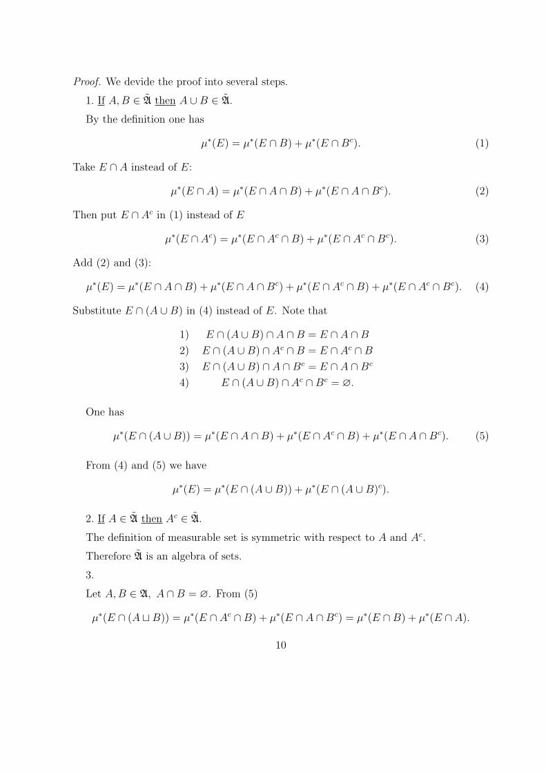
Proof. We devide the proof into several steps.
1. If A, B ∈ A then A ∪B ∈ A.
By the definition one has
µ∗(E) = µ∗(E ∩B) + µ∗(E ∩Bc). (1)
Take E ∩ A instead of E:
µ∗(E ∩ A) = µ∗(E ∩ A ∩B) + µ∗(E ∩ A ∩Bc). (2)
Then put E ∩ Ac in (1) instead of E
µ∗(E ∩ Ac) = µ∗(E ∩ Ac ∩B) + µ∗(E ∩ Ac ∩Bc). (3)
Add (2) and (3):
µ∗(E) = µ∗(E ∩ A ∩B) + µ∗(E ∩ A ∩Bc) + µ∗(E ∩ Ac ∩B) + µ∗(E ∩ Ac ∩Bc). (4)
Substitute E ∩ (A ∪B) in (4) instead of E. Note that
1) E ∩ (A ∪B) ∩ A ∩B = E ∩ A ∩B
2) E ∩ (A ∪B) ∩ Ac ∩B = E ∩ Ac ∩B
3) E ∩ (A ∪B) ∩ A ∩Bc = E ∩ A ∩Bc
4) E ∩ (A ∪B) ∩ Ac ∩Bc = ∅.
One has
µ∗(E ∩ (A ∪B)) = µ∗(E ∩ A ∩B) + µ∗(E ∩ Ac ∩B) + µ∗(E ∩ A ∩Bc). (5)
From (4) and (5) we have
µ∗(E) = µ∗(E ∩ (A ∪B)) + µ∗(E ∩ (A ∪B)c).
2. If A ∈ A then Ac ∈ A.
The definition of measurable set is symmetric with respect to A and Ac.
Therefore A is an algebra of sets.
3.
Let A, B ∈ A, A ∩B = ∅. From (5)
µ∗(E ∩ (A tB)) = µ∗(E ∩ Ac ∩B) + µ∗(E ∩ A ∩Bc) = µ∗(E ∩B) + µ∗(E ∩ A).
10
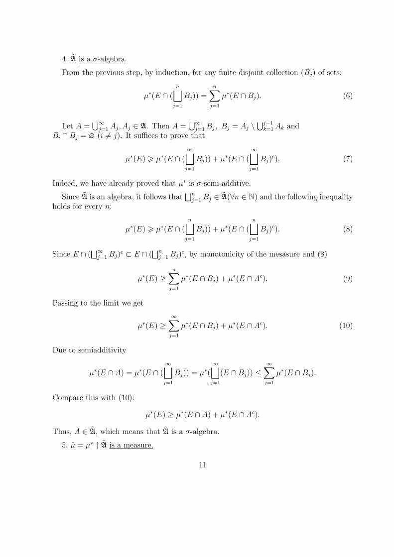
4. A is a σ-algebra.
From the previous step, by induction, for any finite disjoint collection (Bj) of sets:
µ∗(E ∩ (n⊔
j=1
Bj)) =n∑
j=1
µ∗(E ∩Bj). (6)
Let A =⋃∞
j=1 Aj, Aj ∈ A. Then A =⋃∞
j=1 Bj, Bj = Aj \⋃j−1
k=1 Ak andBi ∩Bj = ∅ (i 6= j). It suffices to prove that
µ∗(E) > µ∗(E ∩ (∞⊔
j=1
Bj)) + µ∗(E ∩ (∞⊔
j=1
Bj)c). (7)
Indeed, we have already proved that µ∗ is σ-semi-additive.
Since A is an algebra, it follows that⊔n
j=1 Bj ∈ A(∀n ∈ N) and the following inequalityholds for every n:
µ∗(E) > µ∗(E ∩ (n⊔
j=1
Bj)) + µ∗(E ∩ (n⊔
j=1
Bj)c). (8)
Since E ∩ (⊔∞
j=1 Bj)c ⊂ E ∩ (
⊔nj=1 Bj)
c, by monotonicity of the mesasure and (8)
µ∗(E) ≥n∑
j=1
µ∗(E ∩Bj) + µ∗(E ∩ Ac). (9)
Passing to the limit we get
µ∗(E) ≥∞∑
j=1
µ∗(E ∩Bj) + µ∗(E ∩ Ac). (10)
Due to semiadditivity
µ∗(E ∩ A) = µ∗(E ∩ (∞⊔
j=1
Bj)) = µ∗(∞⊔
j=1
(E ∩Bj)) ≤∞∑
j=1
µ∗(E ∩Bj).
Compare this with (10):
µ∗(E) ≥ µ∗(E ∩ A) + µ∗(E ∩ Ac).
Thus, A ∈ A, which means that A is a σ-algebra.
5. µ = µ∗ � A is a measure.
11
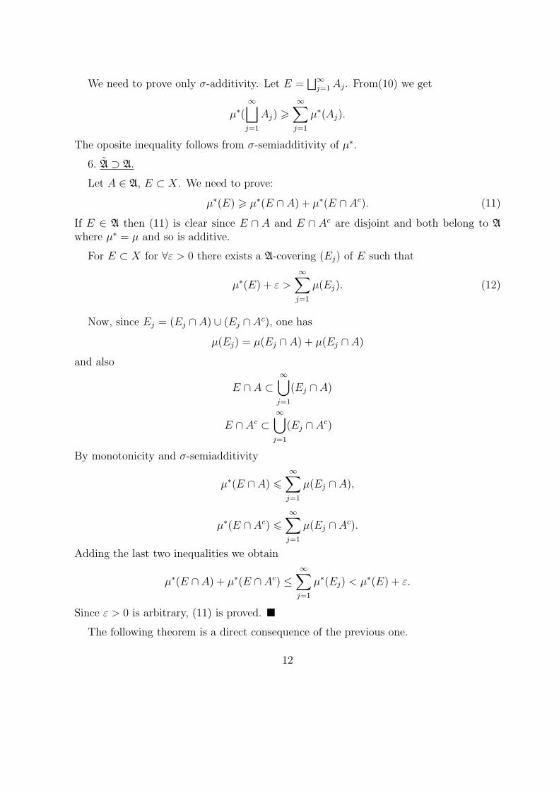
We need to prove only σ-additivity. Let E =⊔∞
j=1 Aj. From(10) we get
µ∗(∞⊔
j=1
Aj) >∞∑
j=1
µ∗(Aj).
The oposite inequality follows from σ-semiadditivity of µ∗.
6. A ⊃ A.
Let A ∈ A, E ⊂ X. We need to prove:
µ∗(E) > µ∗(E ∩ A) + µ∗(E ∩ Ac). (11)
If E ∈ A then (11) is clear since E ∩ A and E ∩ Ac are disjoint and both belong to A
where µ∗ = µ and so is additive.
For E ⊂ X for ∀ε > 0 there exists a A-covering (Ej) of E such that
µ∗(E) + ε >
∞∑j=1
µ(Ej). (12)
Now, since Ej = (Ej ∩ A) ∪ (Ej ∩ Ac), one has
µ(Ej) = µ(Ej ∩ A) + µ(Ej ∩ A)
and also
E ∩ A ⊂∞⋃
j=1
(Ej ∩ A)
E ∩ Ac ⊂∞⋃
j=1
(Ej ∩ Ac)
By monotonicity and σ-semiadditivity
µ∗(E ∩ A) 6∞∑
j=1
µ(Ej ∩ A),
µ∗(E ∩ Ac) 6∞∑
j=1
µ(Ej ∩ Ac).
Adding the last two inequalities we obtain
µ∗(E ∩ A) + µ∗(E ∩ Ac) ≤∞∑
j=1
µ∗(Ej) < µ∗(E) + ε.
Since ε > 0 is arbitrary, (11) is proved. �
The following theorem is a direct consequence of the previous one.
12
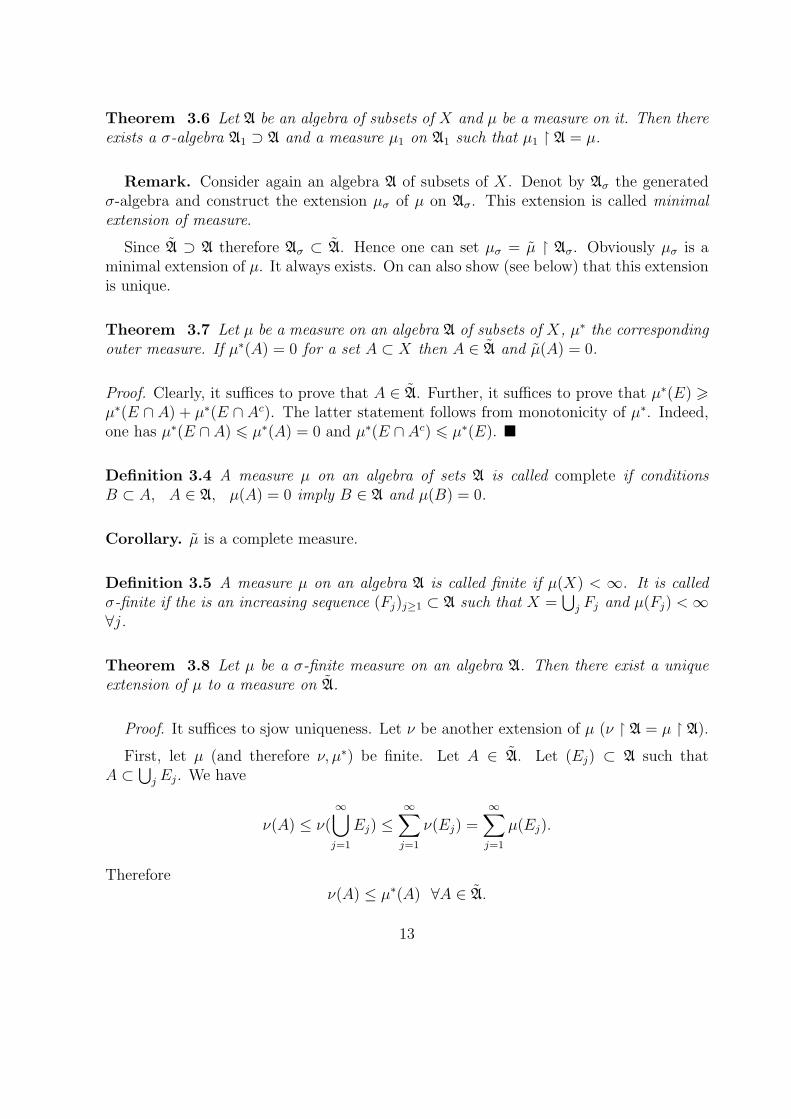
Theorem 3.6 Let A be an algebra of subsets of X and µ be a measure on it. Then thereexists a σ-algebra A1 ⊃ A and a measure µ1 on A1 such that µ1 � A = µ.
Remark. Consider again an algebra A of subsets of X. Denot by Aσ the generatedσ-algebra and construct the extension µσ of µ on Aσ. This extension is called minimalextension of measure.
Since A ⊃ A therefore Aσ ⊂ A. Hence one can set µσ = µ � Aσ. Obviously µσ is aminimal extension of µ. It always exists. On can also show (see below) that this extensionis unique.
Theorem 3.7 Let µ be a measure on an algebra A of subsets of X, µ∗ the correspondingouter measure. If µ∗(A) = 0 for a set A ⊂ X then A ∈ A and µ(A) = 0.
Proof. Clearly, it suffices to prove that A ∈ A. Further, it suffices to prove that µ∗(E) >µ∗(E ∩ A) + µ∗(E ∩ Ac). The latter statement follows from monotonicity of µ∗. Indeed,one has µ∗(E ∩ A) 6 µ∗(A) = 0 and µ∗(E ∩ Ac) 6 µ∗(E). �
Definition 3.4 A measure µ on an algebra of sets A is called complete if conditionsB ⊂ A, A ∈ A, µ(A) = 0 imply B ∈ A and µ(B) = 0.
Corollary. µ is a complete measure.
Definition 3.5 A measure µ on an algebra A is called finite if µ(X) < ∞. It is calledσ-finite if the is an increasing sequence (Fj)j≥1 ⊂ A such that X =
⋃j Fj and µ(Fj) < ∞
∀j.
Theorem 3.8 Let µ be a σ-finite measure on an algebra A. Then there exist a uniqueextension of µ to a measure on A.
Proof. It suffices to sjow uniqueness. Let ν be another extension of µ (ν � A = µ � A).
First, let µ (and therefore ν, µ∗) be finite. Let A ∈ A. Let (Ej) ⊂ A such thatA ⊂
⋃j Ej. We have
ν(A) ≤ ν(∞⋃
j=1
Ej) ≤∞∑
j=1
ν(Ej) =∞∑
j=1
µ(Ej).
Thereforeν(A) ≤ µ∗(A) ∀A ∈ A.
13
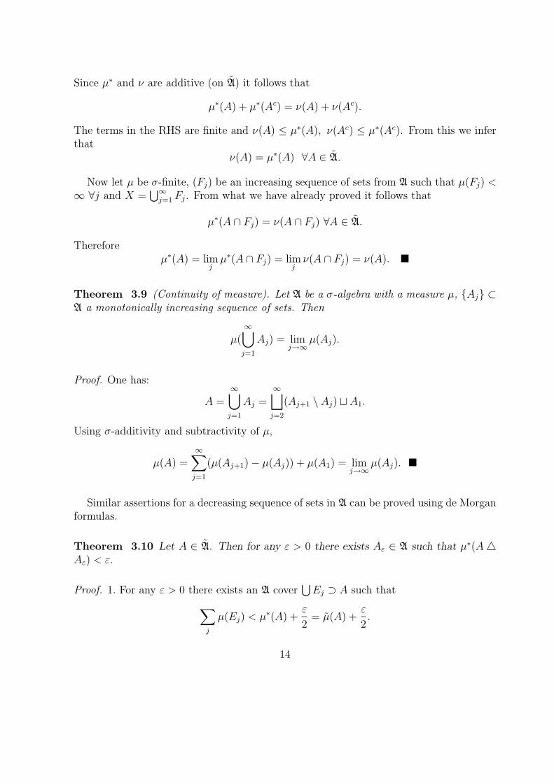
Since µ∗ and ν are additive (on A) it follows that
µ∗(A) + µ∗(Ac) = ν(A) + ν(Ac).
The terms in the RHS are finite and ν(A) ≤ µ∗(A), ν(Ac) ≤ µ∗(Ac). From this we inferthat
ν(A) = µ∗(A) ∀A ∈ A.
Now let µ be σ-finite, (Fj) be an increasing sequence of sets from A such that µ(Fj) <∞ ∀j and X =
⋃∞j=1 Fj. From what we have already proved it follows that
µ∗(A ∩ Fj) = ν(A ∩ Fj) ∀A ∈ A.
Thereforeµ∗(A) = lim
jµ∗(A ∩ Fj) = lim
jν(A ∩ Fj) = ν(A). �
Theorem 3.9 (Continuity of measure). Let A be a σ-algebra with a measure µ, {Aj} ⊂A a monotonically increasing sequence of sets. Then
µ(∞⋃
j=1
Aj) = limj→∞
µ(Aj).
Proof. One has:
A =∞⋃
j=1
Aj =∞⊔
j=2
(Aj+1 \ Aj) t A1.
Using σ-additivity and subtractivity of µ,
µ(A) =∞∑
j=1
(µ(Aj+1)− µ(Aj)) + µ(A1) = limj→∞
µ(Aj). �
Similar assertions for a decreasing sequence of sets in A can be proved using de Morganformulas.
Theorem 3.10 Let A ∈ A. Then for any ε > 0 there exists Aε ∈ A such that µ∗(A4Aε) < ε.
Proof. 1. For any ε > 0 there exists an A cover⋃
Ej ⊃ A such that∑j
µ(Ej) < µ∗(A) +ε
2= µ(A) +
ε
2.
14
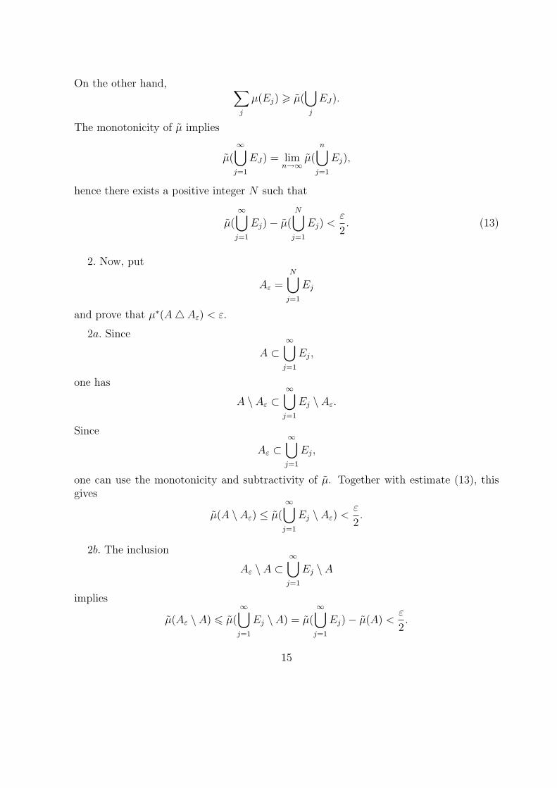
On the other hand, ∑j
µ(Ej) > µ(⋃j
EJ).
The monotonicity of µ implies
µ(∞⋃
j=1
EJ) = limn→∞
µ(n⋃
j=1
Ej),
hence there exists a positive integer N such that
µ(∞⋃
j=1
Ej)− µ(N⋃
j=1
Ej) <ε
2. (13)
2. Now, put
Aε =N⋃
j=1
Ej
and prove that µ∗(A4 Aε) < ε.
2a. Since
A ⊂∞⋃
j=1
Ej,
one has
A \ Aε ⊂∞⋃
j=1
Ej \ Aε.
Since
Aε ⊂∞⋃
j=1
Ej,
one can use the monotonicity and subtractivity of µ. Together with estimate (13), thisgives
µ(A \ Aε) ≤ µ(∞⋃
j=1
Ej \ Aε) <ε
2.
2b. The inclusion
Aε \ A ⊂∞⋃
j=1
Ej \ A
implies
µ(Aε \ A) 6 µ(∞⋃
j=1
Ej \ A) = µ(∞⋃
j=1
Ej)− µ(A) <ε
2.
15
Here we used the same properties of µ as above and the choice of the cover (Ej).
3. Finally,µ(A4 Aε) 6 µ(A \ Aε) + µ(Aε \ A).
�
16
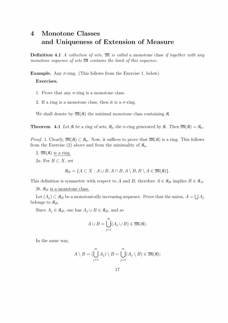
4 Monotone Classes
and Uniqueness of Extension of Measure
Definition 4.1 A collection of sets, M is called a monotone class if together with anymonotone sequence of sets M contains the limit of this sequence.
Example. Any σ-ring. (This follows from the Exercise 1. below).
Exercises.
1. Prove that any σ-ring is a monotone class.
2. If a ring is a monotone class, then it is a σ-ring.
We shall denote by M(K) the minimal monotone class containing K.
Theorem 4.1 Let K be a ring of sets, Kσ the σ-ring generated by K. Then M(K) = Kσ.
Proof. 1. Clearly, M(K) ⊂ Kσ. Now, it suffices to prove that M(K) is a ring. This followsfrom the Exercise (2) above and from the minimality of Kσ.
2. M(K) is a ring.
2a. For B ⊂ X, set
KB = {A ⊂ X : A ∪B, A ∩B, A \B, B \ A ∈ M(K)}.
This definition is symmetric with respect to A and B, therefore A ∈ KB implies B ∈ KA.
2b. KB is a monotone class.
Let (Aj) ⊂ KB be a monotonically increasing sequence. Prove that the union, A =⋃
Aj
belongs to KB.
Since Aj ∈ KB, one has Aj ∪B ∈ KB, and so
A ∪B =∞⋃
j=1
(Aj ∪B) ∈ M(K).
In the same way,
A \B = (∞⋃
j=1
Aj) \B =∞⋃
j=1
(Aj \B) ∈ M(K);
17
B \ A = B \ (∞⋃
j=1
Aj) =∞⋂
j=1
(B \ Aj) ∈ M(K).
Similar proof is for the case of decreasing sequence (Aj).
2c. If B ∈ K then M(K) ⊂ KB.
Obviously, K ⊂ KB. Together with minimality of M(K), this implies M(K) ⊂ KB.
2d. If B ∈ M(K) then M(K) ⊂ KB.
Let A ∈ K. Then M(K) ⊂ KA. Thus if B ∈ M(K), one has B ∈ KA, so A ∈ KB.
Hence what we have proved is K ⊂ KB. This implies M(K) ⊂ KB.
2e. It follows from 2a. — 2d. that if A, B ∈ M(K) then A ∈ KB and so A ∪ B, A ∩ B,A \B and B \ A all belong to M(K). �
Theorem 4.2 Let A be an algebra of sets, µ and ν two measures defined on the σ-algebra Aσ generated by A. Then µ � A = ν � A implies µ = ν.
Proof. Choose A ∈ Aσ, then A = limn→∞ An, An ∈ A, for Aσ = M(A). Using continuityof measure, one has
µ(A) = limn→∞
µ(An) = limn→∞
ν(An) = ν(A).
�
Theorem 4.3 Let A be an algebra of sets, B ⊂ X such that for any ε > 0 there existsAε ∈ A with µ∗(B 4 Aε) < ε. Then B ∈ A.
Proof. 1. Since any outer measure is semi-additive, it suffices to prove that for any E ⊂ Xone has
µ∗(E) > µ∗(E ∩B) + µ∗(E ∩Bc).
2a. Since A ⊂ A, one has
µ∗(E ∩ Aε) + µ∗(E ∩ Acε) 6 µ∗(E). (14)
2b. Since A ⊂ B ∪ (A 4 B) and since the outer measure µ∗ is monotone and semi-additive, there is an estimate |µ∗(A)− µ∗(B)| 6 µ∗(A4 B) for any A, B ⊂ X. (C.f. theproof of similar fact for measures above).
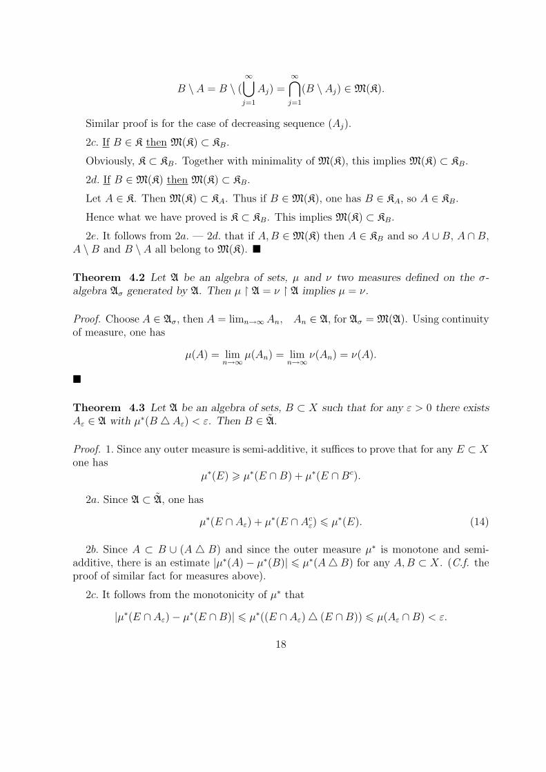
2c. It follows from the monotonicity of µ∗ that
|µ∗(E ∩ Aε)− µ∗(E ∩B)| 6 µ∗((E ∩ Aε)4 (E ∩B)) 6 µ(Aε ∩B) < ε.
18
Therefore, µ∗(E ∩ Aε) > µ∗(E ∩B)− ε.
In the same manner, µ∗(E ∩ Acε) > µ∗(E ∩Bc)− ε.
2d. Using (14), one obtains
µ∗(E) > µ∗(E ∩B) + µ∗(E ∩Bc)− 2ε.
�
19
5 The Lebesgue Measure on the real line R1
5.1 The Lebesgue Measure of Bounded Sets of R1
Put A for the algebra of all finite unions of semi-segments (semi-intervals) on R1, i.e. allsets of the form
A =k⋃
j=1
[aj, bj).
Define a mapping µ : A −→ R by:
µ(A) =k∑
j=1
(bj − aj).
Theorem 5.1 µ is a measure.
Proof. 1. All properties including the (finite) additivity are obvious. The only thing tobe proved is the σ-additivity.
Let (Aj) ⊂ A be such a countable disjoint family that
A =∞⊔
j=1
Aj ∈ A.
The condition A ∈ A means that⊔
Aj is a finite union of intervals.
2. For any positive integer n,n⋃
j=1
Aj ⊂ A,
hencen∑
j=1
µ(Aj) 6 µ(A),
and∞∑
j=1
µ(Aj) = limn→∞
n∑j=1
µ(Aj) 6 µ(A).
3. Now, let Aε a set obtained from A by the following construction. Take a connectedcomponent of A. It is a semi-segment of the form [s, t). Shift slightly on the left itsright-hand end, to obtain a (closed) segment. Do it with all components of A, in such away that
µ(A) < µ(Aε) + ε. (15)
20
Apply a similar procedure to each semi-segment shifting their left end point to the leftAj = [aj, bj), and obtain (open) intervals, Aε
j with
µ(Aεj) < µ(Aj) +
ε
2j. (16)
4. By the construction, Aε is a compact set and (Aεj) its open cover. Hence, there exists
a positive integer n such thatn⋃
j=1
Aεj ⊃ Aε.
Thus
µ(Aε) 6n∑
j=1
µ(Aεj).
The formulas (15) and (16) imply
µ(A) <n∑
j=1
µ(Aεj) + ε 6
n∑j=1
µ(Aj) +n∑
j=1
ε
2j+ ε,
thus
µ(A) <∞∑
j=1
µ(Aj) + 2ε.
�
Now, one can apply the Caratheodory’s scheme developed above, and obtain the mea-sure space (A, µ). The result of this extension is called the Lebesgue measure. We shalldenote the Lebesgue measure on R1 by m.
Exercises.
1. A one point set is measurable, and its Lebesgue measure is equal to 0.
2. The same for a countable subset in R1. In particular, m(Q ∩ [0, 1]) = 0.
3. Any open or closed set in R1 is Lebesgue measurable.
Definition 5.1 Borel algebra of sets, B on the real line R1 is a σ-algebra generated byall open sets on R1. Any element of B is called a Borel set.
Exercise. Any Borel set is Lebesgue measurable.
Theorem 5.2 Let E ⊂ R1 be a Lebesgue measurable set. Then for any ε > 0 thereexists an open set G ⊃ E such that m(G \ E) < ε.
21
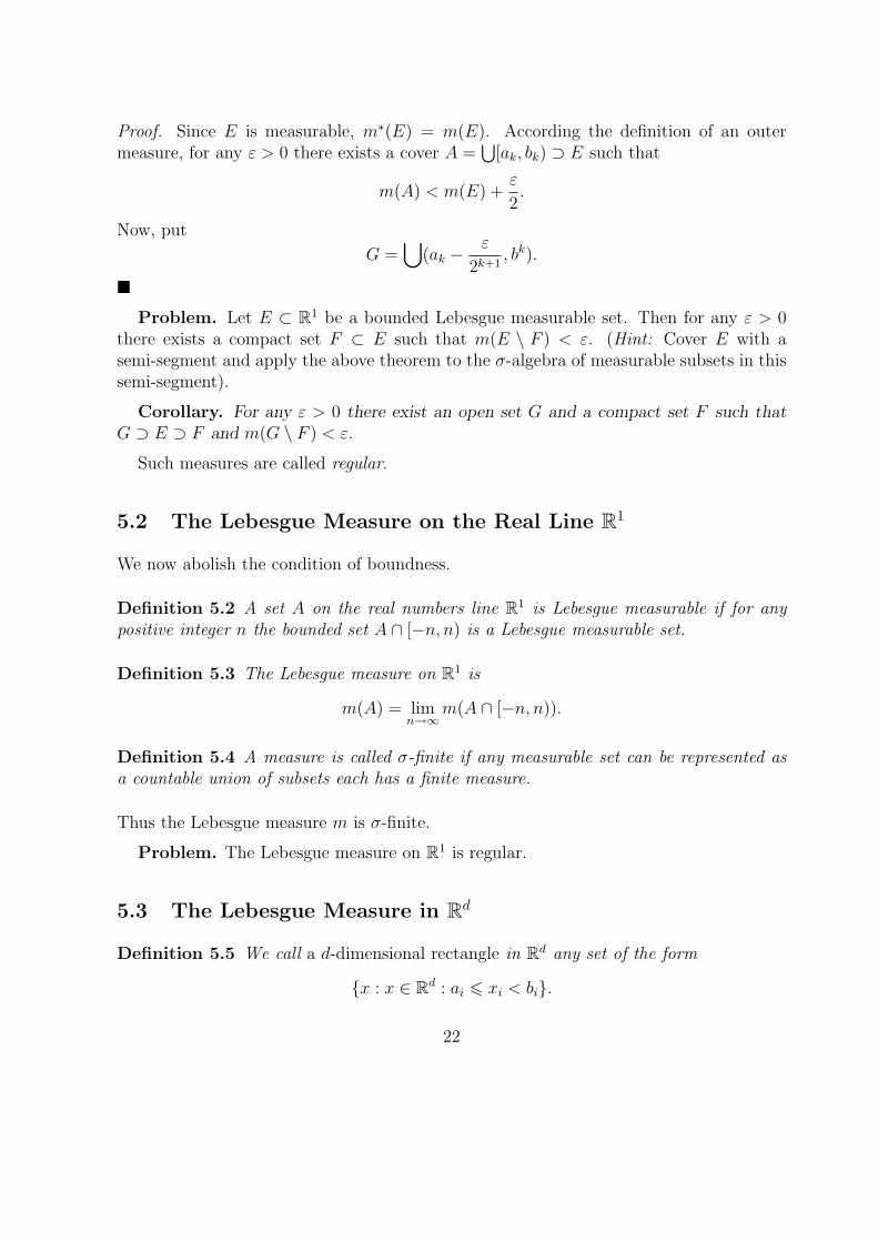
Proof. Since E is measurable, m∗(E) = m(E). According the definition of an outermeasure, for any ε > 0 there exists a cover A =
⋃[ak, bk) ⊃ E such that
m(A) < m(E) +ε
2.
Now, put
G =⋃
(ak −ε
2k+1, bk).
�
Problem. Let E ⊂ R1 be a bounded Lebesgue measurable set. Then for any ε > 0there exists a compact set F ⊂ E such that m(E \ F ) < ε. (Hint: Cover E with asemi-segment and apply the above theorem to the σ-algebra of measurable subsets in thissemi-segment).
Corollary. For any ε > 0 there exist an open set G and a compact set F such thatG ⊃ E ⊃ F and m(G \ F ) < ε.
Such measures are called regular.
5.2 The Lebesgue Measure on the Real Line R1
We now abolish the condition of boundness.
Definition 5.2 A set A on the real numbers line R1 is Lebesgue measurable if for anypositive integer n the bounded set A ∩ [−n, n) is a Lebesgue measurable set.
Definition 5.3 The Lebesgue measure on R1 is
m(A) = limn→∞
m(A ∩ [−n, n)).
Definition 5.4 A measure is called σ-finite if any measurable set can be represented asa countable union of subsets each has a finite measure.
Thus the Lebesgue measure m is σ-finite.
Problem. The Lebesgue measure on R1 is regular.
5.3 The Lebesgue Measure in Rd
Definition 5.5 We call a d-dimensional rectangle in Rd any set of the form
{x : x ∈ Rd : ai 6 xi < bi}.
22

Using rectangles, one can construct the Lebesque measure in Rd in the same fashion aswe deed for the R1 case.
23
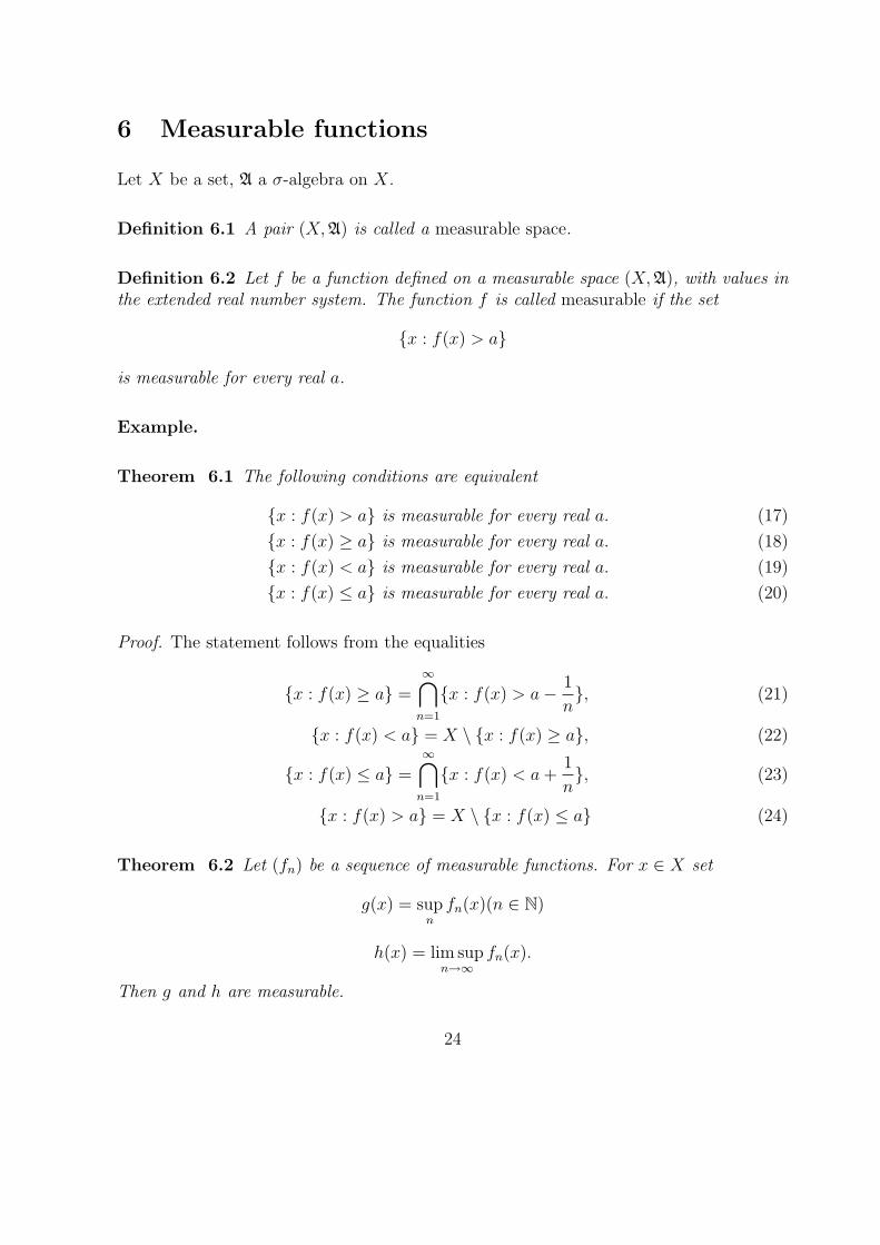
6 Measurable functions
Let X be a set, A a σ-algebra on X.
Definition 6.1 A pair (X, A) is called a measurable space.
Definition 6.2 Let f be a function defined on a measurable space (X, A), with values inthe extended real number system. The function f is called measurable if the set
{x : f(x) > a}
is measurable for every real a.
Example.
Theorem 6.1 The following conditions are equivalent
{x : f(x) > a} is measurable for every real a. (17)
{x : f(x) ≥ a} is measurable for every real a. (18)
{x : f(x) < a} is measurable for every real a. (19)
{x : f(x) ≤ a} is measurable for every real a. (20)
Proof. The statement follows from the equalities
{x : f(x) ≥ a} =∞⋂
n=1
{x : f(x) > a− 1
n}, (21)
{x : f(x) < a} = X \ {x : f(x) ≥ a}, (22)
{x : f(x) ≤ a} =∞⋂
n=1
{x : f(x) < a +1
n}, (23)
{x : f(x) > a} = X \ {x : f(x) ≤ a} (24)
Theorem 6.2 Let (fn) be a sequence of measurable functions. For x ∈ X set
g(x) = supn
fn(x)(n ∈ N)
h(x) = lim supn→∞
fn(x).
Then g and h are measurable.
24
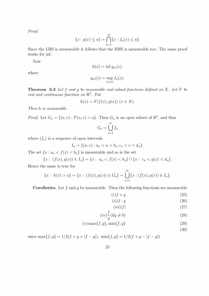
Proof.
{x : g(x) ≤ a} =∞⋂
n=1
{x : fn(x) ≤ a}.
Since the LHS is measurable it follows that the RHS is measurable too. The same proofworks for inf.
Nowh(x) = inf gm(x),
wheregm(x) = sup
n≥mfn(x).
Theorem 6.3 Let f and g be measurable real-valued functions defined on X. Let F bereal and continuous function on R2. Put
h(x) = F (f(x), g(x)) (x ∈ X).
Then h is measurable.
Proof. Let Ga = {(u, v) : F (u, v) > a}. Then Ga is an open subset of R2, and thus
Ga =∞⋃
n=1
In
where (In) is a sequence of open intervals
In = {(u, v) : an < u < bn, cn < v < dn}.The set {x : an < f(x) < bn} is measurable and so is the set
{x : (f(x), g(x)) ∈ In} = {x : an < f(x) < bn} ∩ {x : cn < g(x) < dn}.Hence the same is true for
{x : h(x) > a} = {x : (f(x), g(x)) ∈ Ga} =∞⋃
n=1
{x : (f(x), g(x)) ∈ In}.
Corollories. Let f and g be measurable. Then the following functions are measurable
(i)f + g (25)
(ii)f · g (26)
(iii)|f | (27)
(iv)f
g(ifg 6= 0) (28)
(v) max{f, g}, min{f, g} (29)
(30)
since max{f, g} = 1/2(f + g + |f − g|), min{f, g} = 1/2(f + g − |f − g|).
25
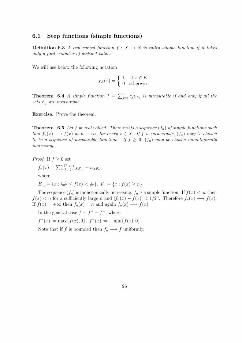
6.1 Step functions (simple functions)
Definition 6.3 A real valued function f : X → R is called simple function if it takesonly a finite number of distinct values.
We will use below the following notation
χE(x) =
{1 if x ∈ E0 otherwise
Theorem 6.4 A simple function f =∑n
j=1 cjχEjis measurable if and only if all the
sets Ej are measurable.
Exercise. Prove the theorem.
Theorem 6.5 Let f be real valued. There exists a sequence (fn) of simple functions suchthat fn(x) −→ f(x) as n →∞, for every x ∈ X. If f is measurable, (fn) may be chosento be a sequence of measurable functions. If f ≥ 0, (fn) may be chosen monotonicallyincreasing.
Proof. If f ≥ 0 set
fn(x) =∑n·2n
i=1i−12n χEni
+ nχFn
where
Eni= {x : i−1
2n ≤ f(x) < i2n}, Fn = {x : f(x) ≥ n}.
The sequence (fn) is monotonically increasing, fn is a simple function. If f(x) < ∞ thenf(x) < n for a sufficiently large n and |fn(x) − f(x)| < 1/2n. Therefore fn(x) −→ f(x).If f(x) = +∞ then fn(x) = n and again fn(x) −→ f(x).
In the general case f = f+ − f−, where
f+(x) := max{f(x), 0}, f−(x) := −min{f(x), 0}.
Note that if f is bounded then fn −→ f uniformly.
26
7 Integration
Definition 7.1 A triple (X, A, µ), where A is a σ-algebra of subsets of X and µ is ameasure on it, is called a measure space.
Let (X, A, µ) be a measure space. Let f : X 7→ R be a simple measurable function.
f(x) =n∑
i=1
ciχEi(x) (31)
andn⋃
i=1
Ei = X, Ei ∩ Ej = ∅ (i 6= j).
There are different representations of f by means of (31). Let us choose the represen-tation such that all ci are distinct.
Definition 7.2 Define the quantity
I(f) =n∑
i=1
ciµ(Ei).
First, we derive some properties of I(f).
Theorem 7.1 Let f be a simple measurable function. If X =⊔k
j=1 Fj and f takes theconstant value bj on Fj then
I(f) =k∑
j=1
bjµ(Fj).
Proof. Clearly, Ei =⊔
j: bj=ciFj.
∑i
ciµ(Ei) =n∑
i=1
ciµ(⊔
j: bj=ci
Fj) =n∑
i=1
ci
∑j: bj=ci
µ(Fj) =k∑
j=1
bjµ(Fj).
�
This show that the quantity I(f) is well defined.
27
Theorem 7.2 If f and g are measurable simple functions then
I(αf + βg) = αI(f) + βI(g).
Proof. Let f(x) =∑n
j=1 bjχFj(x), X =
⊔nj=1 Fj, g(x) =
∑mk=1 ckχGk
(x), X =⊔n
k=1 Gk.
Then
αf + βg =n∑
j=1
m∑k=1
(αbj + βck)χEjk(x)
where Ejk = Fj ∩Gk.
Exercise. Complete the proof.
Theorem 7.3 Let f and g be simple measurable functions. Suppose that f ≤ g every-where except for a set of measure zero. Then
I(f) ≤ I(g).
Proof. If f ≤ g everywhere then in the notation of the previous proof bj ≤ ck on Ejk andI(f) ≤ I(g) follows.
Otherwise we can assume that f ≤ g + φ where φ is non-negative measurable simplefunction which is zero every exept for a set N of measure zero. Then I(φ) = 0 and
I(f) ≤ I(g + φ) = I(f) + I(φ) = I(g).
Definition 7.3 If f : X 7→ R1 is a non-negative measurable function, we define theLebesgue integral of f by ∫
fdµ := sup I(φ)
where sup is taken over the set of all simple functions φ such that φ ≤ f .
Theorem 7.4 If f is a simple measurable function then∫
fdµ = I(f).
Proof. Since f ≤ f it follows that∫
fdµ ≥ I(f).
On the other hand, if φ ≤ f then I(φ) ≤ I(f) and also
supφ≤f
I(φ) ≤ I(f)
which leads to the inequality ∫fdµ ≤ I(f).
�
28
Definition 7.4 1. If A is a measurable subset of X (A ∈ A)and f is a non-negativemeasurable function then we define∫
A
fdµ =
∫fχAdµ.
2. ∫fdµ =
∫f+dµ−
∫f−dµ
if at least one of the terms in RHS is finite. If both are finite we call f integrable.
Remark. Finiteness of the integrals∫
f+dµ and∫
f−dµ is equivalent to the finitenes ofthe integral ∫
|f |dµ.
If it is the case we write f ∈ L1(X, µ) or simply f ∈ L1 if there is no ambiguity.
The following properties of the Lebesgue integral are simple consequences of the defi-nition. The proofs are left to the reader.
• If f is measurable and bounded on A and µ(A) < ∞ then f is integrable on A.
• If a ≤ f(x) ≤ b (x ∈ A)), µ(A) < ∞ then
aµ(A) ≤∫
A
fdµ ≤ bµ(a).
• If f(x) ≤ g(x) for all x ∈ A then∫A
fdµ ≤∫
A
gdµ.
• Prove that if µ(A) = 0 and f is measurable then∫A
fdµ = 0.
The next theorem expresses an important property of the Lebesgue integral. As a con-sequence we obtain convergence theorems which give the main advantage of the Lebesgueapproach to integration in comparison with Riemann integration.
29
Theorem 7.5 Let f be measurable on X. For A ∈ A define
φ(A) =
∫A
fdµ.
Then φ is countably additive on A.
Proof. It is enough to consider the case f ≥ 0. The general case follows from thedecomposition f = f+ − f−.
If f = χE for some E ∈ A then
µ(A ∩ E) =
∫A
χEdµ
and σ-additivity of φ is the same as this property of µ.
Let f(x) =∑n
k=1 ckχEk(x),
⊔nk=1 Ek = X. Then for A =
⊔∞i=1 Ai, Ai ∈ A we have
φ(A) =
∫A
fdµ =
∫fχAdµ =
n∑k=1
ckµ(Ek ∩ A)
=n∑
k=1
ckµ(Ek ∩ (∞⊔i=1
Ai)) =n∑
k=1
ckµ(∞⊔i=1
(Ek ∩ Ai))
=n∑
k=1
ck
∞∑i=1
µ(Ek ∩ Ai) =∞∑i=1
n∑k=1
ckµ(Ek ∩ Ai)
(the series of positive numbers)
=∞∑i=1
∫Ai
fdµ =∞∑i=1
φ(Ai).
Now consider general positive f ’s. Let ϕ be a simple measurable function and ϕ ≤ f .Then ∫
A
ϕdµ =∞∑i=1
∫Ai
ϕdµ ≤∞∑i=1
φ(Ai).
Therefore the same inequality holds for sup, hence
φ(A) ≤∞∑i=1
φ(Ai).
Now if for some i φ(Ai) = +∞ then φ(A) = +∞ since φ(A) ≥ φ(An). So assume thatφ(Ai) < ∞∀i. Given ε > 0 choose a measurable simple function ϕ such that ϕ ≤ f and∫
A1
ϕdµ ≥∫
A1
fdµ− ε,
∫A2
ϕdµ ≥∫
A2
f − ε.
30
Hence
φ(A1 ∪ A2) ≥∫
A1∪A2
ϕdµ =
∫A1
+
∫A2
ϕdµ ≥ φ(A1) + φ(A2)− 2ε,
so that φ(A1 ∪ A2) ≥ φ(A1) + φ(A2).
By induction
φ(n⋃
i=1
Ai) ≥n∑
i=1
φ(Ai).
Since A ⊃⋃n
i=1 Ai we have that
φ(A) ≥n∑
i=1
φ(Ai).
Passing to the limit n →∞ in the RHS we obtain
φ(A) ≥∞∑i=1
φ(Ai).
This completes the proof.�
Corollary. If A ∈ A, B ⊂ A and µ(A \B) = 0 then∫A
fdµ =
∫B
fdµ.
Proof. ∫A
fdµ =
∫B
fdµ +
∫A\B
fdµ =
∫B
fdµ + 0.
�
Definition 7.5 f and g are called equivalent (f ∼ g in writing) if µ({x : f(x) 6=g(x)}) = 0.
It is not hard to see that f ∼ g is relation of equivalence.(i) f ∼ f , (ii) f ∼ g, g ∼ h ⇒ f ∼ h, (iii) f ∼ g ⇔ g ∼ f.
Theorem 7.6 If f ∈ L1 then |f | ∈ L1 and∣∣∣∣∫A
fdµ
∣∣∣∣ ≤ ∫A
|f |dµ
31
Proof.−|f | ≤ f ≤ |f |
Theorem 7.7 (Monotone Convergence Theorem)Let (fn) be nondecreasing sequence of nonnegative measurable functions with limit f. Then∫
A
fdµ = limn→∞
∫A
fndµ, A ∈ A
Proof. First, note that fn(x) ≤ f(x) so that
limn
∫A
fndµ ≤∫
fdµ
It is remained to prove the opposite inequality.For this it is enough to show that for any simple ϕ such that 0 ≤ ϕ ≤ f the followinginequality holds ∫
A
ϕdµ ≤ limn
∫A
fndµ
Take 0 < c < 1. DefineAn = {x ∈ A : fn(x) ≥ cϕ(x)}
then An ⊂ An+1 and A =⋃∞
n=1 An.Now observe
c
∫A
ϕdµ =
∫A
cϕdµ = limn→∞
∫An
cϕdµ ≤
(this is a consequence of σ-additivity of φ proved above)
≤ limn→∞
∫An
fndµ ≤ limn→∞
∫A
fndµ
Pass to the limit c → 1.�
Theorem 7.8 Let f = f1 + f2, f1, f2 ∈ L1(µ). Then f ∈ L1(µ) and∫fdµ =
∫f1dµ +
∫f2dµ
32
Proof. First, let f1, f2 ≥ 0. If they are simple then the result is trivial. Otherwise, choosemonotonically increasing sequences (ϕn,1), (ϕn,2) such that ϕn,1 → f1 and ϕn,2 → f2.
Then for ϕn = ϕn,1 + ϕn,2∫ϕndµ =
∫ϕn,1dµ +
∫ϕn,2dµ
and the result follows from the previous theorem.
If f1 ≥ 0 and f2 ≤ 0 put
A = {x : f(x) ≥ 0}, B = {x : f(x) < 0}
Then f, f1 and −f2 are non-negative on A.
Hence∫
Af1 =
∫A
fdµ +∫
A(−f2)dµ
Similarly ∫B
(−f2)dµ =
∫B
f1dµ +
∫B
(−f)dµ
The result follows from the additivity of integral. �
Theorem 7.9 Let A ∈ A, (fn) be a sequence of non-negative measurable functions and
f(x) =∞∑
n=1
fn(x), x ∈ A
Then ∫A
fdµ =∞∑
n=1
∫A
fndµ
Exercise. Prove the theorem.
Theorem 7.10 (Fatou’s lemma)If (fn) is a sequence of non-negative measurable functions defined a.e. and
f(x) = limn→∞fn(x)
then ∫A
fdµ ≤ limn→∞
∫A
fndµ
A ∈ A
33
Proof. Put gn(x) = infi≥n fi(x)Then by definition of the lower limit limn→∞gn(x) = f(x).Moreover, gn ≤ gn+1, gn ≤ fn. By the monotone convergence theorem∫
A
fdµ = limn
∫A
gndµ = limn
∫A
gndµ ≤ limn
∫A
fndµ.
Theorem 7.11 (Lebesgue’s dominated convergence theorem)Let A ∈ A, (fn) be a sequence of measurable functions such that fn(x) → f(x) (x ∈ A.)Suppose there exists a function g ∈ L1(µ) on A such that
|fn(x)| ≤ g(x)
Then
limn
∫A
fndµ =
∫A
fdµ
Proof. From |fn(x)| ≤ g(x) it follows that fn ∈ L1(µ). Sinnce fn + g ≥ 0 and f + g ≥ 0,by Fatou’s lemma it follows ∫
A
(f + g)dµ ≤ limn
∫A
(fn + g)
or ∫A
fdµ ≤ limn
∫A
fndµ.
Since g − fn ≥ 0 we have similarly∫A
(g − f)dµ ≤ limn
∫A
(g − fn)dµ
so that
−∫
A
fdµ ≤ −limn
∫A
fndµ
which is the same as ∫A
fdµ ≥ limn
∫A
fndµ
This proves that
limn
∫A
fndµ = limn
∫A
fndµ =
∫A
fdµ.
34
8 Comparison of the Riemann
and the Lebesgue integral
To distinguish we denote the Riemann integral by (R)∫ b
af(x)dx and the Lebesgue integral
by (L)∫ b
af(x)dx.
Theorem 8.1 If a finction f is Riemann integrable on [a, b] then it is also Lebesgueintegrable on [a, b] and
(L)
∫ b
a
f(x)dx = (R)
∫ b
a
f(x)dx.
Proof. Boundedness of a function is a necessary condition of being Riemann integrable.On the other hand, every bounded measurable function is Lebesgue integarble. So it isenough to prove that if a function f is Riemann integrable then it is measurable.
Consider a partition πm of [a, b] on n = 2m equal parts by points a = x0 < x1 < . . . <xn−1 < xn = b and set
fm
(x) =2m−1∑k=0
mkχk(x), fm(x) =2m−1∑k=0
Mkχk(x),
where χk is a charactersitic function of [xk, xk+1) clearly,
f1(x) ≤ f
2(x) ≤ . . . ≤ f(x),
f 1(x) ≥ f 2(x) ≥ . . . ≥ f(x).
Therefore the limits
f(x) = limm→∞
fm
(x), f(x) = limm→∞
fm(x)
exist and are measurable. Note that f(x) ≤ f(x) ≤ f(x). Since fm
and fm are simplemeasurable functions, we have
(L)
∫ b
a
fm
(x)dx ≤ (L)
∫ b
a
f(x)dx ≤ (L)
∫ b
a
f(x)dx ≤ (L)
∫ b
a
fm(x)dx.
Moreover,
(L)
∫ b
a
fm
(x)dx =2m−1∑k=0
mk∆xk = s(f, πm)
35
and similarly
(L)
∫ b
a
fm(x) = s(f, πm).
So
s(f, πm) ≤ (L)
∫ b
a
f(x)dx ≤ (L)
∫ b
a
f(x)dx ≤ s(f, πm).
Since f is Riemann integrable,
limm→∞
s(f, πm) = limm→∞
s(f, πm) = (R)
∫ b
a
f(x)dx.
Therefore
(L)
∫ b
a
(f(x)− f(x))dx = 0
and since f ≥ f we conclude that
f = f = f almost everywhere.
From this measurability of f follows. �
36
9 Lp-spaces
Let (X, A, µ) be a measure space. In this section we study Lp(X, A, µ)-spaces which occurfrequently in analysis.
9.1 Auxiliary facts
Lemma 9.1 Let p and q be real numbers such that p > 1, 1p
+ 1q
= 1 (this numbers are
called conjugate). Then for any a > 0, b > 0 the inequality
ab ≤ ap
p+
bq
q.
holds.
Proof. Note that ϕ(t) := tp
p+ 1
q− t with t ≥ 0 has the only minimum at t = 1. It follows
that
t ≤ tp
p+
1
q.
Then letting t = ab−1
p−1 we obtain
apb−q
p+
1
q≥ ab−
1p−1 ,
and the result follows.�
Lemma 9.2 Let p ≥ 1, a, b ∈ R. Then the inequality
|a + b|p ≤ 2p−1(|a|p + |b|p).
holds.
Proof. For p = 1 the statement is obvious. For p > 1 the function y = xp, x ≥ 0 is convexsince y′′ ≥ 0. Therefore (
|a|+ |b|2
)p
≤ |a|p + |b|p
2.�
37
9.2 The spaces Lp, 1 ≤ p < ∞. Definition
Recall that two measurable functions are said to be equaivalent (with respect to themeasure µ) if they are equal µ-a;most everywhere.
The space Lp = Lp(X, A, µ) consists of all µ-equaivalence classes of A-measurablefunctions f such that |f |p has finite integral over X with respect to µ.
We set
‖f‖p :=
(∫X
|f |pdµ
)1/p
.
9.3 Holder’s inequality
Theorem 9.3 Let p > 1, 1p
+ 1q
= 1. Let f and g be measurable functions, |f |p and |g|qbe integrable. Then fg is integrable andthe inequality∫
X
|fg|dµ ≤(∫
X
|f |pdµ
)1/p(∫X
|g|qdµ
)1/q
.
Proof. It suffices to consider the case
‖f‖p > 0, ‖g‖q > 0.
Leta = |f(x)|‖f‖−1
p , b = |g(x)|‖g‖−1q .
By Lemma 1|f(x)g(x)|‖f‖p‖g‖q
≤ |f(x)|p
p‖f‖pp
+|g(x)|q
q‖g‖qq
.
After integration we obtain
‖f‖−1p ‖g‖−1
q
∫X
|fg|dµ ≤ 1
p+
1
q= 1. �
9.4 Minkowski’s inequality
Theorem 9.4 If f, g ∈ Lp, p ≥ 1, then f + g ∈ Lp and
‖f + g‖p ≤ ‖f‖p + ‖g‖p.
38
Proof. If ‖f‖p and ‖g‖p are finite then by Lemma 2 |f + g|pis integrable and ‖f + g‖p
is well-defined.
|f(x)+g(x)|p = |f(x)+g(x)||f(x)+g(x)|p−1 ≤ |f(x)||f(x)+g(x)|p−1+|g(x)||f(x)+g(x)|p−1.
Integratin the last inequality and using Holder’s inequality we obtain∫X
|f+g|pdµ ≤(∫
X
|f |pdµ
)1/p(∫X
|f + g|(p−1)qdµ
)1/q
+
(∫X
|g|pdµ
)1/p(∫X
|f + g|(p−1)qdµ
)1/q
.
The result follows. �
9.5 Lp, 1 ≤ p < ∞, is a Banach space
It is readily seen from the properties of an integral and Theorem 9.3 that Lp, 1 ≤ p < ∞,is a vector space. We introduced the quantity ‖f‖p. Let us show that it defines a normon Lp, 1 ≤ p < ∞,. Indeed,
1. By the definition ‖f‖p ≥ 0.
2. ‖f‖p = 0 =⇒ f(x) = 0 for µ-almost all x ∈ X. Since Lp consists of µ-eqivalenceclasses, it follows that f ∼ 0.
3. Obviously, ‖αf‖p = |α|‖f‖p.
4. From Minkowski’s inequality it follows that ‖f + g‖p ≤ ‖f‖p + ‖g‖p.
So Lp, 1 ≤ p < ∞, is a normed space.
Theorem 9.5 Lp, 1 ≤ p < ∞, is a Banach space.
Proof. It remains to prove the completeness.
Let (fn) be a Cauchy sequence in Lp. Then there exists a subsequence (fnk)(k ∈ N)
with nk increasing such that
‖fm − fnk‖p <
1
2k∀m ≥ nk.
Thenk∑
i=1
‖fni+1− fni
‖p < 1.
39
Letgk := |fn1 |+ |fn2 − fn1|+ . . . + |fnk+1
− fnk|.
Then gk is monotonocally increasing. Using Minkowski’s inequality we have
‖gpk‖1 = ‖gk‖p
p ≤
(‖fn1‖p +
k∑i=1
‖fni+1− fni
‖p
)p
< (‖fn1‖p + 1)p.
Putg(x) := lim
kgk(x).
By the monotone convergence theorem
limk
∫X
gpkdµ =
∫A
gpdµ.
Moreover, the limit is finite since ‖gpk‖1 ≤ C = (‖fn1‖p + 1)p.
Therefore
|fn1|+∞∑
j=1
|fnj+1− fnj
| converges almost everywhere
and so does
fn1 +∞∑
j=1
(fnj+1− fnj
),
which means that
fn1 +N∑
j=1
(fnj+1− fnj
) = fnN+1converges almost everywhere as N →∞.
Definef(x) := lim
k→∞fnk
(x)
where the limit exists and zero on the complement. So f is measurable.
Let ε > 0 be such that for n, m > N
‖fn − fm‖pp =
∫X
|fn − fm|pdµ < ε/2.
Then by Fatou’s lemma∫X
|f − fm|pdµ =
∫X
limk|fnk
− fm|pdµ ≤ limk
∫X
|fnk− fm|pdµ
which is less than ε for m > N . This proves that
‖f − fm‖p → 0 as m →∞. �
40