9 MEASUREMENT OF

CHEMICAL QUANTITIES W.Olthuis

In this chapter, the basics of electrochemical sensing and sensors are described. As is the case with physical sensors in the electrical domain, the retrieved information can be represented by a voltage, a current or an impedance, as shown in Figure 9.1.

For chemical sensors based on electrochemical measuring principles, this sub-division turns out to be a fundamental one because different means of (ionic) mass transport are involved. Information represented by a voltage, a current or an impedance is retrieved by potentiometric sensors, by amperometric sensors or by electrolyte conductivity sensors, respectively.

This determines the outline of this chapter: a section defining some fundamentals is followed by three sections: Potentiometry, Amperometry and Electrolyte Conductivity.

9.1 SOME FUNDAMENTALS AND DEFINITIONS

In this section, several repeatedly used terms are defined [1]. • An electrolyte is a liquid solution through which charge is carried by the

movement of ions.

I

V

Z

Figure 9.1 Any sensor functioning in the electrical domain represents its information as a voltage V, a current I or an impedance Z.

• An electrode is a piece of metal (or semi conductor) through which charge is carried by electronic movement.

• An electrochemical cell is most generally defined as two electrodes separated by an electrolyte.

• The cell potential is the difference in potential across the electrodes of an electrochemical cell.

In an electrochemical cell, often two independent half-reactions take place, each representing the chemical changes at one of two electrolyte/electrode interfaces. Most of the time, we are only interested in one of these two reactions and the electrode at which this occurs is called the working electrode. The remaining electrode is called the reference electrode and is standardized by keeping the concentrations of the species involved in this half-reaction constant. (Nb: the reference electrode is used in potentiometry. For amperometry, another electrode, called the counter electrode, is required. The precise way of using the reference- and counter electrode is beyond the scope of this chapter.) An internationally accepted reference is the normal hydrogen electrode (NHE) where H2 gas at one atmosphere pressure passes a platinum wire via a hollow tube in a solution with pH=0. All these definitions are visualized in Figure 9.2.

9.2 POTENTIOMETRY

Since the reference electrode has a constant makeup, its potential is fixed. Therefore, any changes in the electrochemical cell are ascribed to the working electrode. We say that we observe or control the potential of the working electrode with respect to the reference, and that is equivalent to observing or controlling the energy of the electrons within the working electrode [1]. By driving the electrode to

H2 Ag electrode

Ag+ , NO3-

electrolyte:

half-reaction:

cell potential

Pt electrode

Ag Ag+ + e

in water

(working)(reference, NHE)

Figure 9.2 Visualization of the concept of an electrochemical cell.

more negative potentials the energy of the electrons is raised, and they will eventually reach a level high enough to occupy vacant states on species in the electrolyte. In this case, a flow of electrons from electrode to solution (a reduction current) occurs, resulting in a chemical reaction called reduction. A few examples of reduction reactions, illustrated in Figure 9.3a and b, are

Fe3+ + e → Fe2+ (9.1)

occurring, e.g., at an inert Pt electrode; both Fex+ ions remain dissolved in the electrolyte, and

Ag+ + e → Ag (9.2)

occurring at a silver electrode, now getting thicker from the deposited silver ions.

Similarly, the energy of the electrons can be lowered by imposing a more positive potential, and at some point electrons on solutes in the electrolyte will find a more favourable energy on the electrode and will transfer there. Their flow, from solution to electrode, is an oxidation current. Some examples of oxidation reactions, illustrated in Figure 9.3c and d, are

Fe2+ → Fe3+ + e (9.3)

occurring, e.g., at a Pt electrode; both Fex+ ions remain dissolved in the electrolyte, and

Ag → Ag+ + e (9.4)

Fe3+

Fe3+

Fe2+

Fe2+

Ag+

Ag+

e

ee

Ag

AgPt

Pt

e

Ired Ired

Iox Iox

(a)

(d)(c)

(b)

reduction

oxidation

air

electrolyte

decreasingelectrode potential

increasingelectrode potential

Figure 9.3 Illustration of redox reactions at an electrode in an electrolyte, (a) and (b) representing reduction according to (9.1) and (9.2), respectively, and (c) and (d) representing oxidation according to (9.3) and (9.4), respectively.

occurring at a silver electrode, now getting thinner because of the dissolving silver ions.

It is obvious that (9.1) and (9.2) as well as (9.3) and (9.4) represent identical chemical reactions, only evolving in different directions. This is an interesting observation: lowering an electrode potential causes a reduction current, e.g., according to (9.1) and increasing the potential of this electrode causes the flow of the current to reverse its direction, resulting in a oxidation current, according to (9.3). Obviously, there must exist an electrode potential for which the (net) current is zero! Now what is this potential and how is it related to the chemical reaction of (9.1) and (9.3) and the concentrations of the species involved? This relation between the concentration of chemical species, participating in a redox reaction (= a reaction involving the reduction or oxidation of species) is found by Nernst1.

Let us first generalize (9.1) into:

ox + n.e red (9.5)

where n is the number of electrons involved in the redox reaction. In case there is neither oxidation nor reduction current, (9.5) represents a true equilibrium as indicated by the double arrow. Let us assume that this equilibrium occurs at electrode potential E (always with respect to the potential of the reference electrode, being 0 Volt per definition for a NHE). If we would force the electrode to a potential E’, we would have to use an amount of work to oxidize (if E’ > E) n mol of red into ox that is equal to

( ) [VC/mol] [J/mol]n E E F′ − = (9.6)

in which F equals Faraday's constant2, expressing the amount of Coulomb3 that is present in one mole of electrons: 1.6022.10-19 × 6.0220.1023 = 96484 C/mol. The ratio of the concentrations of red and ox ions in that case is derived from Boltzmann4 statistics, stating that

RTe α− (9.7)

equals the fraction of species (in moles) having an extra energy of at least α. RT [J/mol] is the product of the gas constant R (= 8.314 J/(mol.K) and temperature T. In our case, the species obtain this extra energy by the increased electrode potential. Now, the new ratio in red and ox concentrations can be expressed by substituting the amount of extra work given by (9.6) into (9.7), defining this ratio:

[ ][ ]

'( )n E E FRT

new

oxe

red

− − =

(9.8)

1 Walter Nernst (1864 – 1941), German physical chemist, winner of the Nobel prize in Chemistry in 1920. 2 Michael Faraday, 1791 – 1867, British physicist 3 Charles Augustin Coulomb, 1736 – 1806, French physicist and mathematician 4 Ludwig Boltzmann, 1844 – 1906, Austrian theoretical physicist

where [species] represents the concentration of the species in mol/dm3. It will be no surprise, suggesting that this identity was already valid for the original equilibrium situation of (9.5) with the assumed electrode potential E. In that case with non-existent E’ (=0), (9.8) becomes

[ ][ ]

nEFRT

original

oxe

red

=

(9.9)

or

[ ][ ]ln

oxRTE

nF red

=

(9.10)

dropping the subscript 'original'. This assumed concentration dependent electrode potential E has to be added to the standard potential of an electrode, E0, being the experimentally determined electrode potential under standard conditions for a specific red/ox couple (These standard conditions are: unity concentrations of 1 mol/dm3, at 101.3 kPa and T=298 K). The values of E0 are different for each red/ox couple and can be found in tables.

In conclusion, we derived Nernst Law for any electrochemical reaction of the form ox + ne red being

[ ][ ]

0 lnNernst

oxRTE E

nF red

= +

or

[ ][ ]

0 2.303logNernst

oxRTE E

nF red

⋅= +

(9.11)

By definition, a red or ox species, present in solid form or in gaseous form at atmospheric pressure gets unity (=1) concentration.

This important equation (9.11) is the basis of potentiometry, i.e., measuring the electrode potential with respect to a reference electrode as a function of the concentration of some chemical species in the electrolyte at (almost) zero current.

Example 9.1 From electrode potential to concentration

A silver electrode is immersed in an aqueous solution containing AgNO3. AgNO3 dissolves easily in water. The potential of that electrode is 0.70 V, measured with respect to a Normal Hydrogen reference Electrode at room temperature. What is the concentration of Ag+, present in the solution? The standard electrode potential of the redox reaction Ag+ + e ↔ Ag is E0 = 0.80 V (as tabled in many textbooks, e.g., in [1]). Now substituting the relevant parameters in eq. 9.11 yields:

]1[

][log

96484

298314.8303.280.070.0

+

⋅⋅⋅+= Ag,

or [Ag+]=2.0·10-2 mol/dm3 or 20 mM, being 20 milliMolar, meaning 2.0·10-2 mol/dm3.

Many types of electrodes exist, each requiring a detailed description, not given in this introductory chapter. All potentiometric electrodes, however, can be grouped according to their kind, as summarized in Table 9.1.

Basically, the concentration of a certain ion can be determined by measuring the electrode potential with respect to a reference electrode and using Nernst Law, but only in case one specific redox couple is present in the solution, like the examples mentioned in Table 9.1 for redox electrodes or electrodes of the first or second kind. When more redox couples are present, some mixed potential results, which does not represent the concentration of one specific ion. In all these cases extra membranes have to be engineered and added to the electrode in order to obtain specific information of the concentration of just one ionic species. This results in the last type of electrodes, mentioned in Table 9.1: the Ion Selective Electrodes (ISE).

Some examples:

Fe3+ + e → Fe2+, 3

20.77 lnNernst

FeRTE

F Fe

+

+

= +

, at Pt electrode, redox type;

Pb2+ + 2e → Pb, ( )20.13 ln [ ]2Nernst

RTE Pb

F+= − + , at Pb electrode, first kind;

Cl2 + 2e → 2Cl-, [ ]2

21.36 ln2Nernst

ClRTE

F Cl−

= +

= ( )1.36 ln [ ]RT

ClF

−− , at Pt electrode, redox type.

Basic instrumentation for the measuring of the electrode potential with respect to the reference electrode only consists of a good voltmeter with a very high input impedance (>>1 MΩ), or an impedance transformer (a 'follower') with a high input impedance (>>1 MΩ) and a simple voltmeter. The main concern for the electronic part of the sensor system is to avoid noise, caused by the high source impedance of the electrochemical cell.

When measuring properly, the three given examples yield the following electrode potentials when the Fe3+, the Pb2+ and the Cl- concentration, respectively, is varied (see Figure 9.4). Remember that species present in solid form or in gaseous form at atmospheric pressure get unity concentration (=1) in the Nernst equation, which is here the case for the Pb and the Cl2 concentration. Also, it is

Table 9.1 Overview of electrode types for potentiometry [2] Electrode type Example Redox Pt electrode in Fe3+/Fe2+-containing solution First kind Pb electrode in Pb2+-containing solution Second kind Ag/AgCl electrode in Cl--containing solution Membrane or ISE (Ion Selective Electrode)

Electrode in which a potential difference occurs across a membrane (on top of the electrode); pH glass electrode, NO3

- electrode

assumed that the Fe3+-concentration is varied at constant Fe2+-concentration in Figure 9.4.

9.3 AMPEROMETRY

Amperometry5 is a technique of determining the concentration of an electro-active species via the electrical current that occurs due to the electrochemical reaction of that species at an electrode. Consider a possible redox reaction, e.g.,

Ag+ + e Ag (9.12)

at a silver electrode in an electrolyte, containing Ag+-ions. When we now apply a potential step to the Ag-electrode in negative direction

(lowering the electrode potential with respect to some reference electrode), it is already explained in Section 9.2 that a reduction current will occur (as shown in Figure 9.3b) resulting in a reduction reaction of the equilibrium reaction (9.12):

Ag e Ag+ + → (9.13)

What is happening, is that silver ions from the electrolyte are now reduced to silver atoms and are deposited at the silver electrode, growing thicker. Due to this process, there are less Ag+-ions near the electrode surface than in the bulk of the solution, causing a gradient in Ag+-concentration; from the bulk (higher concentration) to the electrode (lower concentration). Such a gradient causes mass transport by diffusion: movement of a species under the influence of a concentration gradient.

As a result of this mass transport, the Ag+-ions reach the electrode surface at a certain rate (= number of ions per second) and are subsequently reduced to Ag atoms. When we now express the number of ions in moles and normalize this rate 5 after André Marie Ampère, 1775 – 1836, French physicist and mathematician

1e-09 1e-08 1e-07 1e-06 1e-05 1e-04 1e-03 1e-02 1e-01 1e+00

concentration [M]

-0.5

0.0

0.5

1.0

1.5

2.0

elec

trode

pot

entia

l vs.

NH

E [V

] Cl2/Cl-

Fe3+/Fe2+

Pb2+/Pb

Figure 9.4 The electrode potentials of several redox couples as a function of the concentration of the varied species, Cl-, Fe3+ and Pb2+ at room temperature, illustrating Nernst law, equation (9.11).

per unit area, then the so-called flux of Ag+-ions, JAg+, in mol/(m2s) is obtained. Clearly, from (9.13), this flux of silver ions at the electrode surface is related to the reducing current, ired, through the electrode. This current can be easily expressed in the flux of Ag+-ions, JAg+ , by multiplying this flux with the actual electrode area A and Faraday's constant F:

[C/s] [A]red Agi J A F+= − ⋅ = (9.14)

All this is schematically shown in Figure 9.5 in a simplified representation.

Now let us summarize and generalize. The following general reduction reaction occurs at an electrode with a suitable potential:

ox ne red+ → (9.15)

The depletion of ox at the electrode surface causes a concentration gradient of ox, leading to mass transport by diffusion. This results in a flux of ox, Jox that is related to the reduction current, ired, through the electrode with area A according to

red oxi nFAJ= − or redox

iJ

nFA= −

(9.16)

(9.16) is called Faraday’s Law stating that the amount of species involved in the redox reaction, transported by the flux in the electrolyte, is proportional to the amount of charge, transported through the electrode (=electrical current).

Example 9.2 From current to flux

An electric reducing current of 10 μA passes a silver electrode, immersed in an aqueous solution containing plenty of AgNO3 (easily dissolving in water). The electrode area in contact with the solution is 1 mm2. What is the flux of Ag+ ions, JAg+, that reaches the electrode and how many silver ions are reduced to silver per second?

flux JAg+

[Ag+]bulk

concentrationgradient

electrons

ired

reductionAg++e→Agtaking place

Area A Figure 9.5 Impression of the flux caused by the concentration gradient resulting from the reduction of Ag+-ions at the electrode.

Using eq. 9.16 yields: smmolJ Ag24

6

6

/1004.1101964841

1010 −−

−

+ ⋅=⋅⋅⋅

⋅= . In 1 s

on a 1 mm2 electrode, JAg+·1·A·NA = 1.04·10-4·1·1·10-6·6.022·1023 = 6.24·1013 Ag+ ions are being reduced.

Now how can we relate the measured ired to the original concentration of ox in (9.15)? In first approximation, this can be derived and expressed quite easily: ired can be measured and is via (9.16) related to the flux Jox. The driving 'force' for Jox is the concentration gradient of ox near the electrode, so we only have to find an expression for this gradient. For that, Figure 9.6 is used, being a more strict visualization of Figure 9.5.

The flux Jox is linearly related to the concentration gradient via a proportionality constant, Dox, and only one-dimensional diffusion is considered:

( )oxox ox

C xJ D

x

∂= −∂

[mol/ m2s] (9.17)

The minus sign is obvious from Figure 9.6. Dox is the diffusion coefficient, the ease with which the ox particles travel through the electrolyte, and is expressed in m2/s. Combining (9.16) and (9.17) yields an expression relating the measured current ired to the concentration gradient:

( )oxred ox ox

C xi nJ AF nFAD

x

∂= − =∂

[A] (9.18)

Equation (9.18) is generally valid and is called Fick's first law of diffusion6. Now, we make a few assumptions in order to find a simple analytical

expression for the gradient. 1. The slope of the gradient, xCox ∂∂ , is linear, as drawn in Figure 9.6.

6 Adolf Eugene Fick, 1831 – 1879, German physiologist, mathematician and physicist

x

)x(Cox

∂∂ Cox(bulk)

x=0 δ0x [m]

Cox(x)

[M] =[mol/dm3]

Jox

Figure 9.6 Illustration of the flux Jox caused by the gradient xCox ∂∂ , present in the diffusion layer

with thickness δ0.

2. The thickness of the layer in which diffusion takes place is fixed, δ0 in Figure 9.6.

3. The potential of the electrode is such, that Cox(x=0) = 0, i.e., the concentration of ox at the electrode surface drops to zero.

In that case, (9.18) becomes

( ),lim

0 0

( ) ( 0)( )ox ox ox

red iting ox ox

C bulk C x nFADi nFAD C bulk

δ δ− =

= = (9.19)

This is an important equation. It expresses the so-called limiting current for a given species at a certain concentration. It is called 'limiting', because a larger current for the specific reduction reaction of (9.15) is not possible at a fixed bulk concentration Cox(bulk): Jox is at its maximum value. Note from (9.19), that apart from the variable to be measured, Cox(bulk), the diffusion coefficient Dox also determines the limiting current. This value can be found in appropriate tables, or the curve ired = f(Cox(bulk)) can be experimentally determined once with known concentrations of Cox, i.e., the sensor can be calibrated. Obviously, a curve like in Figure 9.7 will then be the result.

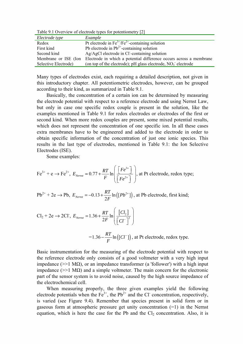
An example of a successful amperometric sensor that is based on the relatively simple equation (9.19), is the oxygen sensor (O2-sensor) as introduced by Clark7. An electrochemical cell, consisting of a Pt disk working electrode and a Ag ring counter electrode in an inner electrolyte solution, as shown in Figure 9.8a and b, is closed by a thin O2-permeable membrane.

7 Leland C. Clark, medical biologist, developed the heart-lung machine and invented the Clark Oxygen Electrode

Cox(bulk) [M]

ired,limiting[μA]

0

oxnFAD

δslope:

Figure 9.7 Illustration of the relation between the limiting current and the bulk concentration.

The Pt working electrode is kept at a potential of –0.7 V versus the Ag/AgCl electrode functioning as counter as well as reference electrode. Oxygen can arrive at this working electrode when it travels through the membrane (slowly, due to the low diffusion coefficient of O2 in the membrane) and the thin layer of electrolyte (fast, due to the high diffusion coefficient of O2 in water). At the electrode, the oxygen will immediately and completely be reduced at –0.7 V according to

O2 + 4e +4H+ → 2H2O

Due to the difference in diffusion coefficient in the membrane and the electrolyte, and the fact that the electrolyte film is even thinner than the membrane, it is reasonable to assume, that the O2-concentration gradient (determining the flux and the reduction current, according to (9.19)) is only present in the membrane and is virtually absent in the thin electrolyte film, as schematically shown in Figure 9.9.

a) b) Figure 9.8 The amperometric oxygen sensor: the Clark electrode; a) cross-sectional view of the total cell; b) a detailed view of the top, showing the membrane and the working and counter electrode.

This makes the Clark electrode successful: the carefully engineered membrane fixes the thickness δ0 in which the O2-gradient is present. Figure 9.10a shows the importance of choosing the correct potential of the Pt working electrode. When the potential is too negative, other interfering redox reactions start to occur, resulting in an increased current. When the potential is not negative enough, not all O2 is completely reduced, causing a partial collapse of the current. The Clark electrode must operate, therefore, at a potential in the plateau region of the current. Only then the measured current truly represents the limiting current according to (9.19). By now, it should be clear that this limiting current increases for higher O2-concentrations, as shown in Figure 9.10b.

Equation (9.19) is not generally valid because of the assumptions we had to make in order to derive (9.19) from (9.18). The weakest assumption is number 2, that of the assumed constant diffusion layer thickness δ0. In reality the thickness of

20 μm 10 μm

O2-permeable membraneinner

electrolyte

Pt working electrode

O2-bulk

0

O2concentration

δ0 of eq 9.19

Figure 9.9 Illustration of the O2-concentration gradient in a Clark electrode, mainly present in the membrane and determined by its thickness δ0.

Figure 9.10 (a) Current versus electrode potential curves for 4 different O2-concentrations, clearly showing the limiting current region at the appropriate electrode potential. 'mm' stands for 'mmHg' and 1 mmHg=133.3 Pa. (b) The limiting current (plateau value) plotted as a function of the partial O2-pressure in %, PO2.

this layer increases in time, making δ a function of time: δ(t). What happens, is schematically shown in Figure 9.11.

Clearly, the slope of the concentration profile

( )( ) ( 0)( )

( )ox oxox

C bulk C xC x

x tδ− =∂ =

∂, with Cox(x=0)=0

(9.20)

decreases for increasing t, because δ(t) increases. Consequently, according to (9.18) and (9.19) the flux and thus the measured current decreases with time, as shown in Figure 9.12.

Unfortunately, there is no longer one constant limiting current for each bulk concentration anymore. Assumption number 1 under (9.18), stating that xCox ∂∂ is thought to be linear is also not true in reality, but the error thus introduced is only a constant factor of 2/√π (ca. 13%). The real, curved concentration profile is shown in Figure 9.13 together with the assumed linear profile.

In order to get rid of the errors, introduced by the assumptions, we need a more rigorous description. For that, some extra mathematics is required, starting with the equation that describes the conservation of matter: the continuity equation:

( , ) ( , )ox oxC x t J x t

t x

∂ ∂= −∂ ∂

(9.21)

Cox(bulk)

t1 t2 t3 t4

t1<t2<t3<t4

δ (t1) δ (t2) δ (t3) δ (t4)

Cox(x)[M]

x [m] Figure 9.11 A more realistic impression of the processes occurring at a current-carrying electrode: the concentration profile develops in time; the diffusion film thickness increases in time.

t [s]

ired(t)[A]

Figure 9.12 The increasing diffusion film thickness causes a decrease in the slope of the concentration gradient (Figure 9.11), resulting in a decreased flux and electrode current as illustrated here.

This equation represents the change in concentration per second being equal to the change in flux per meter; [mol/(s.m3)] and can easily be illustrated with Figure 9.14. The change in concentration at x (in compartment Δx) can only be caused by the difference in flux into and flux out of this compartment:

( , ) ( , ) ( , )ox ox oxC x t J x t J x x t

t x

∂ − + Δ=∂ Δ

Letting Δx approach zero results in (9.21). Note that x)t,x(J ox ∂∂ has dimensions of mol/(m3s), being a change in concentration per unit time, as required. Combining (9.17) and (9.21) yields Fick's second law of diffusion:

2

2

( , ) ( , )ox oxox

C x t C x tD

t x

∂ ∂= ∂ ∂

(9.22)

0

Figure 9.13 Illustration of a minor correction: discontinuous gradients in one medium do not occur in reality. Curve 2 is nice for modelling, curve 1 is closer to reality.

Jox(x,t) Jox(x+∆x,t)

∆x

x x+∆x Figure 9.14 Illustration used for the determination of the continuity equation, (9.21), leading to Fick's second law of diffusion, equation (9.22).

If we now presume a planar electrode (e.g., a platinum disk at x=0) and an unstirred solution [1], we can calculate the diffusion-limited current, ired, using eq. 9.22 and the following boundary conditions:

( , 0) ( )ox oxC x t C bulk= = (9.23)

lim ( , ) ( )ox oxxC x t C bulk

→∞= (9.24)

( 0, ) 0oxC x t= = (for t>0) (9.25)

The initial condition (9.23) merely expresses the homogeneity of the solution before the experiment starts at t=0, and the semi-infinite condition (9.24) is an assertions that regions sufficiently distant from the electrode are unperturbed by the experiment. The third condition, (9.25), expresses the surface condition after the (negative, reducing) potential step, resulting in sudden, complete depletion of ox-particles at the electrode surface.

The solution of (9.22), using conditions (9.23)- (9.25) can be obtained after Laplace transformation, resulting in a mathematical expression for Cox(x,t). This expression (not given here) can be substituted in (9.23), producing the current-time response by using (9.18):

( ) oxox

Di t nFAC

tπ=

(9.26)

which is known as the Cottrell equation8. As with every equation, having its own name, this is an important one. The meaning and practical use of the Cottrell equation (9.26) for amperometric concentration determination will be illustrated with the following example [3]. In Figure 9.15a several current versus time responses are shown for different concentrations of hydrogen peroxide, H2O2. The involved reduction reaction is

2 2 22 2 2H O H e H O++ + → (9.27)

This reaction, and thus the reduction current as shown in Figure 9.15a occur at a Pt working electrode of 0.5 cm2 when stepping from 0 to –0.5 V (versus a so-called Ag/AgCl reference electrode).

To show that we are really dealing with the phenomena as predicted by Cottrell, we plot the curves of Figure 9.15a again, but now against 1/√t, because (9.26) then predicts straight lines:

( )1

oxox

Di tnFA C

tπ

∂ =∂

[As1/2] (9.28)

8Frederick Gardner Cottrell, 1877 – 1948, American analytical chemist; the equation was published in 1902

with different slopes for each different H2O2 concentration. Figure 9.15b confirms this prediction. The slopes of these curves are plotted in Figure 9.16, now as a function of the applied H2O2 concentration, giving the calibration curve for this sensor.

From the Cottrell equation, the diffusion coefficient can be determined as a

verification:

2 2

2

H O

slopeD

nFAπ =

= 1.62.10-9 m2/s

which is equal to the theoretical value of 1.6.10-9 m2/s. In conclusion: this type of amperometric sensing appears to be a reliable

method for the detection of the hydrogen peroxide concentration. This approach can also be applied for other redox couples, present in the solution, as long as they

0 1 2 3 40 0

20 20

40 40

60 60

Time [sec]0 1 2 3

Cur

rent

[A

]

Time [ sec ]

Cur

rent

[A

]

2 mM

2 mM

4 mM

4 mM

6 mM

6 mM

8 mM

8 mM

10 mM

10 mM

(a) (b)

-1 -1

Figure 9.15 Chrono amperometric H2O2 measurement results:(a) the current relaxation curves at a Pt electrode for several H2O2 concentrations, (b) the same data but plotted on a non-linear time axis

0 5 100

5

10

15

20

25

30

Sensor type ASensor type B

[H O ] (mM)

It

(A

sec

2 2 Figure 9.16 Measured calibration curve for chrono amperometric responses for two different Pt electrodes.

are alone. However, when other redox-active species are also present, concentration information about one ion specifically can only be obtained by adding a selective membrane to the electrode

9.4 ELECTROLYTE CONDUCTIVITY

9.4.1 Faradaic and Non-faradaic Processes

Two types of processes occur at electrodes [1]. One kind comprises those just discussed in the previous section, in which charges (i.e., electrons) are transferred across the metal-solution interface. This electron transfer causes oxidation or reduction. Since these reactions are governed by Faraday's law (i.e., the amount of species involved in the redox reaction, transported by the flux in the electrolyte, is proportional to the amount of charge, transported through the electrode (=electrical current), they are called faradaic processes. Electrodes at which faradaic processes occur are sometimes called charge transfer electrodes. Under some conditions a given electrode-solution interface will show a range of potentials where no charge transfer reactions occur because such reactions are thermodynamically or kinetically unfavourable. These processes are called non-faradaic processes. Although charge does not cross the interface under these conditions, external currents can flow (at least transiently) when the potential changes. We discuss now the case of a system where only non-faradaic processes occur: electrolyte conductivity sensing.

Electrolyte Conductivity (EC) sensing nowadays is a well-established and much practiced technique of measuring. After an introduction of the basic concept of EC sensing, the relevant equations to describe conductivity are presented. An additional topic of this section is to treat several options for increasing the reliability of EC sensing.

Electrolyte conductivity (EC) is an expression for the mobility and concentration of ions in an aqueous solution as a result of an electric field [4]. For the determination of EC, a voltage difference must be present between two conducting electrodes, placed in the solution. This difference in potential results in an electric field between the electrodes causing the mobile ions to migrate. The resulting ionic mass transport manifests itself at the conducting electrodes as an electronic current, known or measurable.

Ionic mass transport can take place by three different means, each governed by a different driving force, as indicated in Table 9.2. It will be clear that the only mode of mass transport, involved in EC is migration.

Table 9.2 Modes of ionic mass transport with their driving forces modes driving force diffusion difference in concentration, concentration gradient migration difference in electric potential, potential gradient, electric field convection difference in density, stirring

9.4.2 Theoretical background of EC sensing

Relevant equations and definitions[4] The underlying ionic transport mode of EC is migration. The driving force of migration is a potential gradient, dV/dx, or electric field E:

dx

dVE −= [V/m]

(9.29)

This electric field imposes an electric force, Fe, on every charge particle, i.e., every ion:

e iF z qE= [N] (9.30)

with zi the valence of ion i, and q the electronic charge. The ion will accelerate until the frictional drag (due to the viscosity of the medium) exactly counter balances the electric force. Then, the ion travels at a constant velocity, v. At this velocity, the ion experiences a frictional or drag force, Fd, equal to

6dF rvπη= [N] (9.31)

with η the viscosity of the medium and r the ionic radius. This situation is depicted in Figure 9.17.

At constant velocity, Fe=Fd, and from (9.30) and (9.31) the mobility of the ion i, μi, is defined:

6i

i

z qv

E rμ

πη= = [m/s per V/m ≡ m2/(Vs)]

(9.32)

The resulting ionic mass transport flux by migration, Ji, using (9.29) is

i i i

dVJ C

dxμ= − [mol/(m2s)]

(9.33)

with Ci the concentration of ion i [mol/m3]. The resulting electronic current density, due to all n ions that are present in the solution is

+ FeFd

v

medium E

+ -

Figure 9.17 The force balance experienced by a charged particle under the influence of an applied electric field, E, in a viscous medium, resulting in a constant travelling speed, v.

1

n

i i ii

dVJ F z C

dxμ

=

= [A/m2] (9.34)

When the electric field E=dV/dx is linear between two electrode plates with electrode area A and distance , as depicted in Figure 9.18, the electronic current can be obtained:

1

n

i i ii

Vi JA FA z Cμ

=

Δ= =

[A] (9.35)

with ΔV the potential difference that is present between the electrodes.

Example 9.3 Ion velocity due to migration What is the maximum velocity of a silver ion in an aqueous solution migrating between two plan-parallel electrodes placed =1 mm apart with 0.1 VRMS over these electrodes?

The mobility of Ag+-ions is tabled in text books: μAg+=6.43·10-8 m2/sV at room temperature. Velectrode= 0.1 VRMS means ΔVelectrode= 0.141 Vtop.

Using eqs. 9.29 and 9.32 the maximum velocity v = μAg+·E= μAg+·(ΔVtop/) = 6.43·10-8·(0.141/1·10-3)=9.1·10-6 m/s=9.1 μm/s.

Now, the conductance G can be expressed using (9.35):

1

1 n

i i ii

i FAG z CR V

μ=

= = =Δ

[Ω-1] = [S]iemens (9.36)

with R is the resistance. The conductance G is a variable that can be measured, and depends on the type and dimensions of the electrodes. To be independent on these system parameters, the conductivity κ can be defined as

1Gkκ

ρ= = [Ω-1m-1]

(9.37)

with ρ [Ωm] the resistivity, and k [m-1] the system parameter, called the cell-constant. In the case of two plan-parallel electrodes shown in Figure 9.18 with area A and distance , k=/A as can be derived from (9.36) and (9.37). So, from these equations, the expression for the conductivity, κ, is

1

n

i i ii

F z Cκ μ=

= [Ω-1m-1] (9.38)

For solutions of simple, pure electrolytes (i.e., one positive and one negative ionic species, like KCl or CaCl2) the conductivity can be normalized with respect to its equivalent concentration of positive (or negative) charges, Ceq, from which the equivalent conductivity Λeq can be obtained:

eqeqC

κΛ = [Ω-1m2/mol of charge] (9.39)

with Ceq=|Ci|zi. From (9.38) and (9.39), Λeq can be expressed as

( )eq F μ μ+ −Λ = + (9.40)

with μ+, μ- the cationic and anionic mobility, respectively. This equation leads to the definition of equivalent ionic conductivity, λi,eq:

,i eq iFλ μ= [Ω-1m2/mol of charge] (9.41)

Note, that following the same line of reasoning a molar conductivity, Λm, and a molar ionic conductivity, λi,m, can be defined:

m C

κΛ = [Ω-1m2/mol of species] (9.42)

with C [mol/m3] the concentration of the added species and

,i m i iF zλ μ= [Ω-1m2/mol of species] (9.43)

Sensing of EC For a proper understanding of practical EC determination, it is necessary to introduce the electrode-solution interface before continuing.

l

∆Vi

A

Figure 9.18 Illustration of two plan-parallel electrodes with electrode area A and distance . The cell-constant for this conductivity sensor is k=/A [m-1].

In Figure 9.19 a complete, two-electrode EC sensor is schematically depicted. As explained, a voltage applied over the two electrodes would result in an electric current due to the migrating ions as a result of the electric field that is caused. It will be explained that EC can not be successfully determined by a DC voltage over the electrodes.

Scenario 1 The applied DC voltage is that high, that redox reactions at the electrodes will occur and current flows via Rdiffusion through the faradaic path of Figure 9.19. Possible reactions in a solution of NaCl in water are, e.g.,:

at the anode, +, 2Cl- → Cl2 +2e

at the cathode, -, 2H2O + 2e → 2OH- + H2

In this case, however, the concentrations of mobile ions contributing to the EC (Cl- and OH-, in this example), changes at the proximity of the electrode, giving rise to mass transport by diffusion. Thus, a proper EC determination in which only transport by migration is allowed, is no longer possible.

Scenario 2 The applied DC voltage is low enough to avoid any redox reactions. In this case, however, the charge on the conducting electrode that is present due to the applied voltage, will almost immediately be counteracted by an equal amount of ionic charge, of opposite sign, in the solution at the direct proximity of the electrode. Of course, it are these two charges that form the well-known double layer capacitance, also present in Figure 9.19. But now, the potential applied over the electrode, with respect to the solution, will be present over Cdl only: no longer over the solution itself, thus inhibiting any migration due to the absence of the driving force; the electric field.

From this discussion, it may be clear that EC can only be determined properly by applying an AC voltage over the electrode with such an amplitude, that redox processes are avoided, and with such a frequency, that the impedance of Cdl is of the order of, or much smaller than the Rel to be determined, to allow a practical and precise EC determination.

Figure 9.19 Schematic model of a two-electrode EC sensor. Rel represents the measured electrolyte resistance, Rdiffusion and Cdl the (simplified) faradaic pathway electrode resistance and the non-faradaic pathway electrode double layer capacitance, respectively.

9.4.3 Extra reliability

Reliability at EC sensing means the unambiguous determination of Rel of Figure 9.20.

Theoretically, this can be accomplished by carefully taking into account the electrode-solution interface impedance, schematically depicted by Rdiffusion and Cdl of Figure 9.20. This impedance, however, is by no means a constant and ideal element, but varies with the concentration of the electrolyte, its composition, and also with the electrical potential and frequency over the electrode-solution interface. Therefore, a practically more feasible approach is to design the EC sensor in such a way, that the electrode-solution interface impedance influences the total impedance of the sensor (as shown in Figure 9.19) as minimally as possible. Two options are elaborated in the next sub-sections.

Use of Pt-black electrodes By a proper (electro)chemical treatment, the otherwise shiny surface of a Pt electrode can become black due to the thus obtained cauliflower-like structure. The resulting rough surface can be characterized by its original geometric electrode surface area, Ageometric and by its effective surface area, Aeffective, as schematically depicted in Figure 9.21.

Figure 9.20 Simplified representation of the electrode-solution interface impedance, including the electrolyte resistance, Rel.

Aeffective

Pt-blackelectrode

Ageometric

Rel

Cdl

determined byAgeometric

determined byAeffective

a) b) Figure 9.21 a) A Pt-black electrode can be characterized by its geometric electrode area, Ageometric and the real area, including the surface area of all micro-structures, Aeffective.; b) increasing the roughness of the electrode surface decreases the impedance of the double layer capacitance, leaving the electrolyte resistance unaffected, resulting in a more precise determination of Rel at a given measurement frequency.

Remember, that at proper operation, Rdiffusion of Figure 9.20 is absent, because only migrational effects via Cdl are involved in EC determination. Now, the effect of the Pt black electrode can be easily explained. The electrolyte resistance, Rel of Figure 9.21b, is determined by the electrode area Ageometric and is not affected by the rough surface and remains constant at constant electrolyte concentration. The double layer capacitance, Cdl, however, is determined by the rough electrode surface and thus by Aeffective. As the impedance of Cdl (=1/jωCdl ÷ 1/Aeffective) dramatically decreases with a likewise dramatically increasing Aeffective with respect to Ageometric, due to the Pt-black formation, the impedance of Cdl can virtually be neglected with respect to Rel at a suitable measuring frequency. Thus, the goal as stated at the start of this section: an unambiguous determination of Rel, by decreasing the effect of the interface impedance, is obtained.

However, by fouling and/or degeneration of the initial rough Pt surface, the ratio Aeffective / Ageometric gradually decreases, thereby lowering the favourable effect of the treatment. Moreover, the Pt black electrode is mechanically rather weak, making (mechanical) cleaning not very well possible. Therefore, periodic regeneration of the Pt black electrode is necessary in order to keep its favourable behaviour.

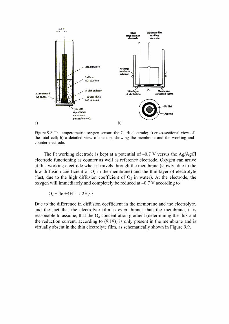
The conventional 4-points EC measurement A well-known alternative to the previously described approach is the 4-points measuring method, as schematically depicted in Figure 9.23 (see Section 7.1.4).

By separating the current injection electrodes from the voltage measurement electrodes, the voltage drop over the electrode impedance, Zelectrode in Figure 9.22, is no longer present in the measured potential. Moreover, as there are no longer strict demands on the current electrodes, they can be designed very small.

Also this method, however, has some disadvantages. Firstly, the design of the probe is more complicated due to the increased number of electrodes and their interrelation. Secondly, the design and implementation of the electronics is also a bit more complicated. Thirdly, the signal-to-noise ratio of the whole sensor plus electronics is a critical and difficult to tackle parameter, due to the high impedance of the potential sensing electrodes.

potentialmeasurement

current injection

Zelectrode ZelectrodeRelectrolyte

Figure 9.22 A typical electrical representation of a 4-points EC probe, showing the separate current injection and potential sensing electrodes and, more importantly, the position of the unfavourable electrode impedance, Zelectrode, with respect to the potential sensing electrodes.

Example 9.5 EC sensing with an interdigitated electrode pair

One of the common manifestations of an EC sensor is the so-called interdigitated conductivity electrode [4]. Especially in small (chemical micro-)systems, the planar structure is an advantage. Moreover, this device can be fabricated in a clean room with usual photolithographic techniques. A typical lay out of such a device is depicted in Figure 9.23a.

The overall dimensions are 1 x 1 mm2. In reality, the device consists of 9 fingers in total. In order to minimize the interfering effect of the double layer impedance, the operating frequency had to be chosen at 200 kHz. The result of a set of measurements in different potassium nitrate (KNO3) concentrations is shown in Figure 9.23b. Here, the reciprocal value of Rel is plotted as a function of the concentration, because then a linear dependence is expected (and obtained). The calculation of the cell constant of such an interdigitated structure is a mathematically complicated task, not repeated here [5]. The calculated cell constant of this device is 1.28 cm-1 and the experimentally determined value is 1.24 cm-1.

9.5 FURTHER READING

Allen J. Bard; Larry R. Faulkner, Electrochemical methods: fundamentals and applications, New York [etc.]: Wiley, 2nd ed. (2001); ISBN: 0-471-04372-9 hbk This excellent book is not a standard textbook concerning electrochemical sensors as such, but a very fundamental and at the same time well-readable book about all possible electrochemical aspects on electrode – solution interfaces and much more.

9.6 REFERENCES

[1] A.J.Bard, L.R.Faulkner: Electrochemical methods, fundamentals and applications, John Wiley and Sons, New York, 1980

[2] B.J.Birch, T.E.Edmonds: Potentiometric transducers, in: Chemical Sensors, ed. by T.E. Edmonds, Blackie and son, Glasgow and London, 1988

Z

0

0.5

1.0

1.5

2

0 5 1510 20

Concentration KNO

Adm

itta

nce

of R

[m

S]

3 [mM]

El-1

a) b) Figure 9.23 a) Impression of an interdigitated electrolyte conductivity electrode; b) admittance versus potassium-nitrate concentration, measured at 200 kHz. The range from 0.5 to 20 mM KNO3 is equivalent to 0.072 to 2.9 mS/cm.

[3] G.R.Langereis: An integrated sensor system for monitoring washing processes, PhD-thesis, University of Twente, ISBN 90-365-1272-7, 1999

[4] W.Olthuis, P.Bergveld: Reliability and selectivity at electrolyte conductivity sensing. Biocybernetics and biomedical engineering, 19 (1), 1999

[5] W.Olthuis, W.Streekstra, P.Bergveld: Theoretical and experimental determination of cell constants of planar-interdigitated electrolyte conductivity sensors. Sensors and Actuators B (Chemical), 24-25, 1995

9.7 EXERCISES

1. What is the dimension of RT/F? What is the quantity of RT/F at room temperature (T=298K)?

2. Why is measuring the electrode potential using a voltmeter with relatively low input impedance not wise in potentiometry? 3. What is the potential difference between a silver electrode and an aluminium electrode, immersed in an aqueous solution at room temperature containing 50·10-3 mol/dm3 AgNO3 and 20·10-3 mol/dm3 Al(NO3)3? 4. What is the flux of electrons at a distance of 1 meter from an electron emitter, spraying electrons homogeneously in all directions? A current of 1 μA is applied to the emitter. 5. An O2-sensitive Clark electrode is used in an aqueous solution in which 5 millimol/dm3 of O2 is dissolved. The measured limiting current is 4 μA. The thickness of the O2-permeable membrane is 20 μm and the surface area of the Pt-electrode is 1 mm2. Calculate the diffusion coefficient DO2 of oxygen in the membrane. 6. Referring to example 9.2, what is the electrochemical deposition rate of Ag on the electrode (expressed in thickness increase per time)? Additional data: 1 mol Ag weighs 0.108 kg and 1 m3 Ag weighs 7.9·103 kg. 7. Conductivity is temperature dependent. What parameter causes this temperature dependence and will the conductivity increase or decrease when raising the temperature? 8. Express the capacitance C and the resistance R of the configuration of Figure 9.18, using its cell-constant, in case a block of material is placed between the electrodes with relative permittivity εr and resistivity ρ. In addition, derive the expression for the RC-product. What is the dimension of RC? 9. Check the experimentally determined curve shown in Figure 9.23b for [KNO3]=10 mM, knowing that μK+=7.62·10-8 m2/sV, μNO3-=7.40·10-8 m2/sV at T=298 K and the cell-constant is k=1.24 cm-1.