UPTEC F15 017

Examensarbete 30 hpApril 2015

Measurement of dispersion barriers through SEM images

Basel Aiesh

Teknisk- naturvetenskaplig fakultet UTH-enheten Besöksadress: Ångströmlaboratoriet Lägerhyddsvägen 1 Hus 4, Plan 0 Postadress: Box 536 751 21 Uppsala Telefon: 018 – 471 30 03 Telefax: 018 – 471 30 00 Hemsida: http://www.teknat.uu.se/student

Abstract

Measurement of dispersion barriers through SEMimages

Basel Aiesh

In this thesis digital image analysis is applied to Scanning Electron Microscope imagesof dispersion barriers to measure specific properties. The thin barriers are used asprotection for paperboard packaging and are made of polymers and fillers. Theorientation, area, length and density distributions of the fillers determine thefunctionality and quality of the barrier. Methods built on image analysis tools aredeveloped with the objective to measure these quantities. Input for the methods areScanning Electron Microscope images showing the cross-section of the barriers. Tomake the images relevant for the methods they are preprocessed by reducing noiseand distinguishing fillers from the background.

For measuring the orientation distribution of the fillers two different methods areimplemented and compared. The first one is based on a structure tensor and theother one applies a covariance matrix. The structure tensor is preferable because ofits flexibility and better performance for complex images. The area and lengthdistributions are measured by applying mathematical morphology together withsoft-clipping. The density distribution is obtained by filtering the underlying imagetwice with a uniform filter which creates a heat map.

The developed methods are evaluated by applying them on fabricated binary testimages with known properties. The methods are very accurate when applied onsimple test images but for more complex test images with greater variation theaccuracy decreases. However, for most applications the results are still on anacceptable level.

ISSN: 1401-5757, UPTEC F15 017Examinator: Tomas NybergÄmnesgranskare: Ida-Maria SintornHandledare: Cris Luengo, Åsa Nyflött

Contents 1 Introduction 1

1.1 Background . . . . . . . . . . . . . . . . . . . . . . . . . . . . . 1

1.2 Assignment . . . . . . . . . . . . . . . . . . . . . . . . . . . . . 1

2 Theoretical background 3

2.1 Circular mean . . . . . . . . . . . . . . . . . . . . . . . . . . . . 3

2.2 Structure tensor . . . . . . . . . . . . . . . . . . . . . . . . . . . . 3

2.3 Morphological opening . . . . . . . . . . . . . . . . . . . . . . . . 4

2.3.1 Area opening . . . . . . . . . . . . . . . . . . . . . . . . . . 5

2.3.2 Path opening . . . . . . . . . . . . . . . . . . . . . . . . . . 5

2.4 Granulometry . . . . . . . . . . . . . . . . . . . . . . . . . . . . 5

2.5 Soft-clipping . . . . . . . . . . . . . . . . . . . . . . . . . . . . . 6

2.6 Student’s t-test . . . . . . . . . . . . . . . . . . . . . . . . . . . . 7

3 Methods 8

3.1 Preprocessing . . . . . . . . . . . . . . . . . . . . . . . . . . . . . 8

3.1.1 Suppressing noise . . . . . . . . . . . . . . . . . . . . . . . . 9

3.1.2 Automatic segmentation . . . . . . . . . . . . . . . . . . . . 9

3.1.3 Manual segmentation . . . . . . . . . . . . . . . . . . . . . 10

3.2 Orientation distribution . . . . . . . . . . . . . . . . . . . . . . . 11

3.2.1 Covariance Matrix method . . . . . . . . . . . . . . . . . . 12

3.2.2 Structure Tensor method . . . . . . . . . . . . . . . . . . . 12

3.3 Area distribution and length distribution . . . . . . . . . . . . . . . 14

3.3.1 Soft-clipping . . . . . . . . . . . . . . . . . . . . . . . . . 14

3.3.2 Granulometry . . . . . . . . . . . . . . . . . . . . . . . . 15

3.4 Density distribution and density gradient . . . . . . . . . . . . . . 16

3.4.1 Density distribution . . . . . . . . . . . . . . . . . . . . . . 16

3.4.2 Density gradient . . . . . . . . . . . . . . . . . . . . . . . 16

4 Evaluation of methods 18

4.1 Orientation evaluation . . . . . . . . . . . . . . . . . . . . . . 18

4.1.1 Sigma dependency of Structure Tensor method . . . . . . . . . 18

4.1.2 Object based vs. pixel based approach . . . . . . . . . . . . . 18

4.1.3 Error estimation . . . . . . . . . . . . . . . . . . . . . . . 20

4.2 Area and length distribution . . . . . . . . . . . . . . . . . . . . . 23

4.3 Density distribution . . . . . . . . . . . . . . . . . . . . . . . . . 25

4.3.1 Pixel error . . . . . . . . . . . . . . . . . . . . . . . . . . 25

4.3.2 Image error . . . . . . . . . . . . . . . . . . . . . . . . . . 27

4.3.3 Calculation time comparison of filters . . . . . . . . . . . . . 27

5 Results & Discussion 28

5.1 Running the program . . . . . . . . . . . . . . . . . . . . . . . . 28

5.2 Example output . . . . . . . . . . . . . . . . . . . . . . . . . . . 28

5.3 Discussion of results . . . . . . . . . . . . . . . . . . . . . . . . 31

6 Conclusions 34

Acknowledgements . . . . . . . . . . . . . . . . . . . . . . . . . . . . 35

References . . . . . . . . . . . . . . . . . . . . . . . . . . . . . . . . . 36

Appendix A . . . . . . . . . . . . . . . . . . . . . . . . . . . . . . . . 38

1

Chapter 1

Introduction 1.1 Background

The packaging industry is a huge business sector and annually makes billions of dollars in

revenues. It is of great significance for the companies to produce functional packaging made of high quality. Nowadays it is becoming more and more important to create effective solutions that consume less energy and are environmentally sustainable. Several different research projects have been accomplished on this topic and many are still running. Today the packaging industry relies heavily on the use of materials produced from finite resources. This is not defensible in the long term, neither from an economic perspective nor from an environmental perspective. While the accessibility of finite resources is decreasing, the costs are increasing making it non-profitable to use in the future. Also the waste disposal problems in some areas will worsen and must be taken into consideration.

Some frequently used food packaging materials today are plastic, metal and glass but the most

common are paper and paperboard packaging [1]. This is due to their light weight which gives them beneficial properties when it comes to storing and transporting. In addition to that they are advantageous from a carbon footprint view in the recycling process. The packaging and their content need protection from different substances such as gases, moisture and dust. It is also important that water, grease or packaging gases do not penetrate to the outside. One way to achieve this is to coat the packaging with a thin barrier. There are several different coating techniques today such as extrusion, wax coating and barrier coating [2].

Barrier coatings are made of high-quality polymers and are sometimes filled with fillers. The

coating layer improves convertibility and creates effective barriers with desirable properties. One special type of barrier coating is the dispersion barrier which is produced by polymers and fillers mixed in water. A dispersion differs from a regular solution because the particles in the water are not dissolved as they would be in a solution, but they rather stay intact. The dispersion barrier is applied to the packaging surface and is dried into solid form. There are several different techniques for both the application and the drying of the barrier [3].

1.2 Assignment

Scanning Electron Microscope (SEM) images showing the cross section of dispersion barriers are investigated using image analysis tools. Examples of some SEM images are given in Figure 1.1. Be aware that only (a) is showing the cross section while (b) displays a perpendicular view. The latter image is of no practical use for this thesis, but rather included for clarity. The bright

2

objects appearing are a form of clay fillers and are the interesting parts of the images. This thesis aims at analyzing the orientation, area, length and density distributions of the fillers in the SEM images. For this purpose, image analysis is used and different methods are developed. Since there is no ground truth for the SEM images, the methods should be evaluated by running them on synthetic test images with known properties.

The different distributions are important to measure because they determine the functionality

and quality of the dispersion barrier. For a barrier to have an optimal protection it is desirable for the fillers to possess some specific properties. They should be aligned with the barrier surface and evenly distributed in the barrier. Furthermore long thin particles that give a high aspect ratio for the particles are preferred. By striving towards these properties the tortuosity factor of the barrier will increase which means that the ability for external substances to flow through the barrier decreases [4].

The work in this thesis is limited to method development and evaluation. The results gained

when the methods are applied on the SEM images should only be reflected at a very basic level. Thus, functionality and quality of the barriers are not to be examined or compared.

(a) (b)

Figure 1.1: Images of dispersion barriers containing clay fillers taken with a Scanning Electron Microscope. (a) Cross section of barrier. (b) As seen from above.

3

Chapter 2

Theoretical background

This chapter goes through the theory that is relevant for the methods in this thesis. It is assumed that the reader understands basic image analysis theory, so fundamental subjects such as Gaussian filtering, segmentation or morphological operations will not be treated

2.1 Circular mean

When calculating the mean of a periodical dataset, using the arithmetic mean is not always

optimal. For example the arithmetic mean between the angles 0 , and is . For most

applications this result is not desirable because 0 and are the same orientations and the

preferred result should be 0 (or . By calculating the circular mean instead this problem can be avoided.

The circular mean converts all the angles in a dataset from polar coordinates to

complex numbers [5]. The arithmetic means of the complex

numbers are calculated, generating one final complex number. The argument of this number is the circular mean

where is the th element of a weight function If no weights are used for all k.

2.2 Structure tensor

A tensor is a mathematical object that occurs in several different applications. The order of a tensor is determined by the number of indices needed to describe each element in the tensor. For example a scalar is a tensor of order zero since it does not need any indices and a vector has the

order of one since an element in a vector needs exactly one index. Using the

same logic, a matrix consequently is a tensor of order two. One special case of such a tensor is the structure tensor which is derived from the gradients of a function. The outer product of the gradients is the foundation of the structure tensor. Another name that often occurs in the literature is the second-moment matrix.

The first step for calculating a structure tensor of an image is to suppress noise and to

determine its gradient field. Since an image is a discrete valued function the gradient field can

4

only be computed approximately. If the image is convolved by a Gaussian filter (called just a Gaussian from now on) initially the approximation will improve, but it is still an approximation. This thesis applies a different approach called Gaussian derivates [6]. That is, rather than computing the gradient of the image convolved with a Gaussian, the gradient of the Gaussian is convolved with the image. Mathematically, that is

where and are grayscale images, is a Gaussian and is

the convolution operator. The gradient of the Gaussian can be calculated analytically. Sampling it into a filter and convolving with the image, the exact gradient of a blurred version of the image is calculated. In other words, this does not calculate the real gradient of the original image and is thus also an approximation. But a Gaussian is probably needed anyhow to remove noise so the Gaussian derivates are favorable compared to other methods.

The outer product of the gradient vector

is computed. This yields a symmetric

positive semi-definite matrix, called the field matrix [7]:

where the subscripts denote partial derivatives. The structure tensor for a certain neighborhood

of scale is then computed by convolution with a Gaussian kernel

.

The structure tensor holds information about the local orientation and the local anisotropy in

a neighborhood shaped by . The eigenvectors and the eigenvalues of the tensor are computed and sorted in descending order. The anisotropy is computed as the ratio

between the eigenvalues, . For the neighborhood is fully

isotropic. The largest eigenvalue determines the strength of the eigenvector which points in

the direction of the gradient. The local orientation is perpendicular to and is therefore

determined by where serves as a certainty measure.

2.3 Morphological opening

Mathematical morphology is a wide and well documented area within the image analysis field with plenty of applications. This thesis uses two types of morphological operations, area opening and path opening. These methods are rather advanced compared to basic morphological operations. It’s not necessary within the frame of this thesis to dig into their underlying theory and therefore they are described very briefly in the forthcoming text. The interested reader is referred to [8, 9] for area opening and [10, 11, 12] for path opening.

5

2.3.1 Area opening

Using a filter to remove connected components smaller than a certain area from an image is called area opening. Computing area openings on binary images is a straightforward task. Labeling the connected components and then studying the histogram of the image will provide the area of each of its components. A size parameter determines which components that are too small and removes them. The SEM images in this thesis are as we know not binary but grayscale and therefore more sophisticated methods are needed. There are numerous different algorithms for this end and the one used in this thesis is based on Vincent’s proposition in [9]. In short, the strategy is to first find regional maxima for the image. Then the neighboring pixels are scanned and added to the growing region where higher intensities have higher priority. In other words, the regional threshold around each maximum is lowered. The process stops when the number of pixels scanned are larger than a certain area and finally all pixels within the region are given the value of the latest pixel scanned.

2.3.2 Path opening

In analogy with area opening, a path opening is used when we want to remove structures from an image based on their lengths. The path opening has a structure element that consists of a flexible but constrained line segment that is able to adapt locally to the image’s structures. This property is especially suitable when dealing with elongated objects that are not necessary straight. In this thesis the path opening is performed according to the algorithm suggested by Luengo [12]. It is a simplification of Appleton and Talbot’s algorithm [11] that gives it a slight increase in execution time but at the same time makes the algorithm dimension independent.

2.4 Granulometry

A granulometry or morphological sieve is in image analysis an approach that applies multi scale morphological openings or closings on an image [13]. Which operation to use depends on the relative intensity between the objects and the background. Openings are used for light objects and closings for dark ones. For this reason, only openings are concerned in this thesis. The objective is to find a size distribution of some property for the objects in the image. As an analogy to a granulometry, one can think of the size distribution determination of physical sediment grains. In this case physical sieves with different mesh sizes are used, starting with a large sieve and repeatedly using smaller sieves on the remainder of the grains. Finally the grains are sorted by size in their respective sieve. By weighing each fraction of the grains a size distribution is received. A normalized distribution can be obtained by comparing each fraction to the total weight.

Let define a two-dimensional grayscale image and a structure element of size .

Performing separate morphological openings on the image with increasing size of the structure element results in the scale space

where is the opening operator and is the size of the :th structure element. For each scale,

the opening eliminates objects where the structure element does not fit. The acquired image after

6

each opening is integrated, e.g. the sum of all intensities is computed. This

contributes to a cumulative distribution where each increment is represented by the integration of a scale image.

The distribution inherits the rotation and translation invariant characteristics from the opening operation. Further on by normalizing the distribution it also gets independent of the image size and contrast, as well as the area ratio between the image and the objects. The normalized

cumulative distribution is defined as

where is the original image and is the result of an opening with an infinite structure element size, which in most cases basically means that the image is filled with its minimum intensity. An ordinary normalized size distribution can be obtained by computing the

derivative of with a first order approximation

.

This is sometimes referred to as the pattern spectrum. The strength of the morphological sieve is that it can operate directly on the grayscale image without any preprocessing. However, the intensities of the objects in the image most likely are not uniform. This leads to weighing errors in the granulometry when integrating over the scale images, so a preprocessing method that minimizes these deviations is needed. In the following section such a method is presented.

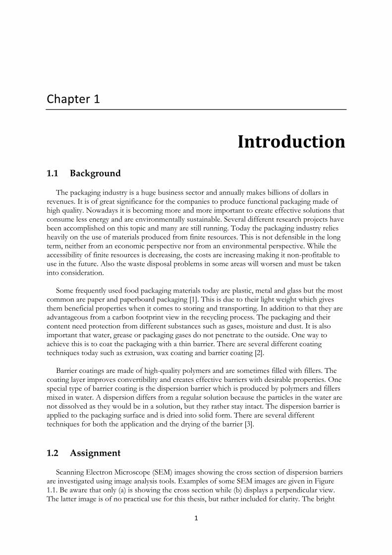
2.5 Soft-clipping

Soft-clipping, or error-function clipping, is a technique that cuts off an image (1-dim for

simplicity) at two different thresholds, a low and a high . Apart from hard-clipping the

cutoffs for soft-clipping are not flat. Instead they are stretched according to

where

is the intensity halfway between the thresholds and

is the error function [13]. Figure 2.2 shows the principle of clipping. The black

sinusoidal curve represents an image, the blue lines the hard-clipped image and the red curves the soft-clipped. Soft-clipping is an appropriate preprocessing step to implement before computing the granulometry of an image.

7

Figure 2.2: Illustration of soft-clipping (red) and hard-clipping (blue) of a one dimensional image (black).

2.6 Student’s t-test

The Student's t-distribution (or just t-distribution) is a continuous probability distribution that emerges when estimating the mean of a normally distributed population [14]. A normal distribution describes the full population while a t-distribution describes a sample of it. The two distributions are very similar in shape and the larger the sample the more the t-distribution resembles a normal distribution.

A Student’s t-test is a statistical hypothesis test in which the test statistic follows a t-distribution if the null hypothesis is supported. It can be applied for different scenarios in statistics but in this thesis it is used as a one-sample test. The null hypothesis reads; the mean of a population of estimated errors equals zero. The equation that tests this at a 95% significance level is

where is the sample mean, is the hypothesized population mean, is the sample standard

deviation, and is the sample size. Under the null hypothesis, the test statistic has a t-distribution with degrees of freedom.

8

Chapter 3

Methods

This chapter aims at explaining the methods designed for this thesis. Their purpose is to measure the orientation, area, length and density distributions of the fillers appearing in the SEM images. All the methods were implemented in MATLAB® (The MathWorks, Natick, Massachusetts, http://www.mathworks.com/) supported by the Image Processing ToolboxTM and DIPimage (Delft University of Technology, Delft, The Netherlands, http://www.diplib.org/) Both these are practical toolboxes consisting of useful functions for image analysis tasks.

SEM images showing the cross sections of dispersion barriers serve as input for the methods.

In Figure 3.1 two different SEM images are presented. The fillers appearing in different sizes and forms are henceforth for image applications to be addressed as “objects”.

Figure 3.1: Two examples of cross section SEM images of dispersion barriers

3.1 Preprocessing In almost all image analysis applications the images need to be preprocessed in order for them

to be qualitative meaningful for the computer. It is an essential step in the image analysis process that should be evaluated before proceeding. The preprocessing task in this thesis is to suppress the noise and to distinguish between the background and the objects in the images. The latter is in technical terms called that we want to segment the images.

9

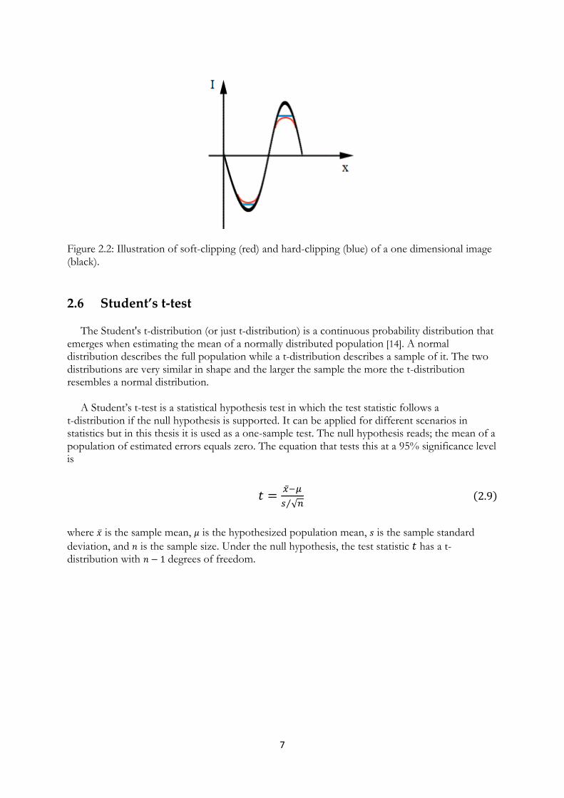
3.1.1 Suppressing noise The input images contain noise generated from the acquisition and must be filtered with some

sort of noise suppressing filter. Since the noise is random, a Gaussian filter is suitable. The filtering operation results in smoother objects and a more homogeneous background. This is illustrated in Figure 3.2 where a noisy small segment of a SEM image is filtered with two different Gaussians.

(a) (b) (c)

Figure 3.2: (a) A noisy segment of a SEM image. (b) Same image filtered with a Gaussian with

and a kernel size of 5. (c) Filtered with a Gaussian with and a kernel size of 5.

3.1.2 Automatic segmentation

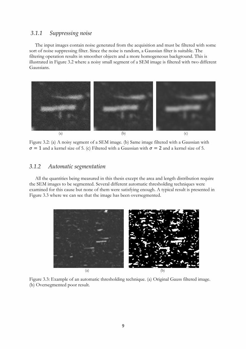
All the quantities being measured in this thesis except the area and length distribution require the SEM images to be segmented. Several different automatic thresholding techniques were examined for this cause but none of them were satisfying enough. A typical result is presented in Figure 3.3 where we can see that the image has been oversegmented.

(a) (b)

Figure 3.3: Example of an automatic thresholding technique. (a) Original Gauss filtered image. (b) Oversegmented poor result.

10

3.1.3 Manual segmentation

Instead of using an automatic segmentation technique, a simple threshold approach that analyzes the image’s intensity histogram was implemented. It is based on the assumption that the

most common intensity belongs to the background. A decent threshold value should hence be found somewhere to the right of this intensity in the histogram. By extracting the maximum

intensity and introducing a scale factor the threshold is calculated as

All the intensities below the threshold represent the background and are set to zero. The rest of the pixels keep their intensities or alternatively they get the value one which creates a binary image. Which option to choose depends on the application and in the coming example the former option is selected. For the threshold application to give a nice result an appropriate scale factor needs to be found. This is done empirically by comparing the results of different thresholds. Nevertheless a fixed value that works acceptable for most of the images in this thesis can be found and applied.

A typical SEM image histogram and an enlarged version are presented in Figure 3.4(a b). After finding a suitable scale factor and applying the threshold the histogram in (c) is obtained. All intensities below the threshold have been set to zero and left are the intensities belonging to the objects. Figure 3.5 illustrates the results using three different scale factors. In (b) where a low scale factor has been used the objects are too thick and sometimes merged with other objects. In (d) a lot of the objects are removed as a result of the scale factor being too high. A satisfying result is showed in (c) where the scale factor is somewhere between the two previous ones.

(a) (b) (c)

Figure 3.4: Different views of a SEM image’s intensity histogram. (a) The full original histogram. (b) Zoomed view of original histogram. (c) Zoomed view after applying threshold.

11

(a) (b)

(c) (d)

Figure 3.5: Examples showing on the dependency of the scale factor when segmenting objects in a SEM image. (a) Original image. (b) Threshold to low. (b) An acceptable threshold. (d) Threshold too high

3.2 Orientation distribution

Two different methods were developed to estimate the orientations of the objects in the SEM images. The first one is named the Covariance Matrix (CM) method and operates on binary images by computing the spread of pixels for each object. The other method is called the Structure Tensor (ST) method and applies a structure tensor that calculates local orientations on a normalized version of the preprocessed image. An example output that displays the orientation distribution of the objects is shown in Figure 3.6. An average orientation value of the objects may be practical and can easily be extracted from the distribution by computing the circular mean of all object orientations, as explained in section 2.1.

Figure 3.6: Example output for the ST method or the CM method showing the orientation distribution of objects in a SEM image.

12

3.2.1 Covariance Matrix method The CM method relies on the image to be segmented properly. The strategy for this was

explained in section 3.1. After a binary version of the image has been obtained the objects are labeled and their orientations are ready to be determined. Each object is represented by a covariance matrix that is defined as

where [15]. are the coordinates of the object and

is its mean. This matrix can be interpreted as the spread distribution of the pixels within an object and can be represented by a visionary ellipse that has the same covariance matrix as the current object. By extracting the eigencomposition of the matrix the axes of the represented ellipse can

be obtained. The orientation is defined to be the angle between the major axis of the ellipse and an imaginary horizontal line. An illustrating example is shown in Figure 3.7.

(a) (b)

Figure 3.7: The principle of the CM method. (a) An object represented with an ellipse that carries an identical covariance matrix as the object. (b) Orientation of object defined as angle between the ellipse’s major axis and the horizon.

3.2.2 Structure Tensor method

The ST method determines the orientation of an object by gaining local information for each pixel within the object. Taking the average over the concerned pixels gives an estimate for the orientation of the object and an object based orientation distribution can be produced. An alternative and more flexible strategy that can be advantageous is to base the distribution directly on the local orientations. However, for this to compute the mean orientation of all objects correctly it needs to be weighted because larger objects contribute more to the distribution than smaller ones. This weighing was not implemented because the object based approach should be adequate for the applications in this thesis.

Figure 3.8(a) demonstrates what an input for the ST method may look like. This image is gained by setting the background to zero in the original Gauss filtered SEM image as explained in the preprocessing section. In Figure 3.8(b) a normalized version of this image is presented. By comparing the two images one can see that the normalized image is smoother and that the contrast between background and foreground is fuzzier. Please aware that even though some objects seem to have disappeared due to their dark shade, they are all present. Also note the difference in intensity scale.

13

(a) (b)

Figure 3.8: (a) Example of input image for the ST method where the background pixels have been set to zero. (b) Input image that has been normalized.

A structure tensor is applied on the normalized image which produces the images displayed in

Figure 3.9(a b). They illustrate all the pixels’ local orientations and local anisotropies respectively. The orientations are given in radians and the anisotropies are always a value between zero and one. These images need to be manipulated before averaging. This is done by pixel-wise multiplying them with a binary segmented version of the original image. The resulting products are one image illustrating the objects with their local orientations and another image showing the

anisotropic counterpart; see Figure 3.9(c d). The circular mean with the anisotropies as weights is used to take the average over each object and hence an object based orientation distribution can be acquired.

(a) (b)

(c) (d)

Figure 3.9: Local orientations and anisotropies for a SEM image computed by the ST method. (a) Local orientations. (b) Local anisotropies. (c) Local orientations after cutting out objects. (d) Local anisotropies after cutting out objects.

14

3.3 Area distribution and length distribution

The area and length distributions of the objects in the SEM images are estimated by applying a set of morphological operations with structure elements of increasing size. This functions as a sieve that removes objects smaller than the structure element. The result is a size distribution of the desired property also known as a granulometry.

3.3.1 Soft-clipping

An object in an image commonly exists of wide spread intensities with descending values towards the edges. There probably also are differences between the objects; some are darker while others are lighter. Since a granulometry is based on the sum of intensity values, these deviations lead to weighing errors for the estimated size distribution. It would be preferable if all the objects had similar intensities and likewise for the background. This can be achieved by applying soft-clipping, described in section 2.4.

The threshold values for the soft-clipping are computed in the same way as the preprocessing threshold earlier in this chapter. An assumption that the most common intensity belongs to the background is made. From this value two thresholds are derived, a low and a high. This is done

by determining the factor or in the equation

where are the thresholds, the most common intensity and is the maximum intensity. Given the thresholds, soft-clipping can now be applied on the original image.

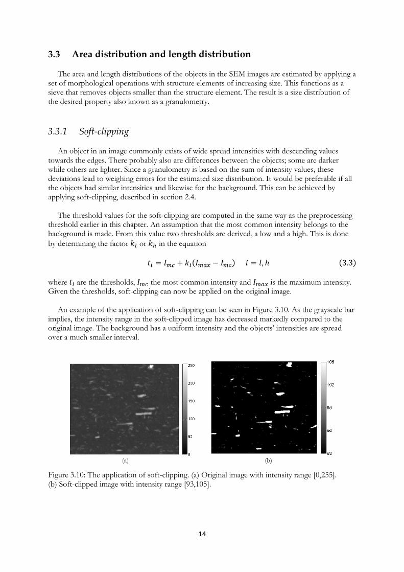
An example of the application of soft-clipping can be seen in Figure 3.10. As the grayscale bar

implies, the intensity range in the soft-clipped image has decreased markedly compared to the original image. The background has a uniform intensity and the objects’ intensities are spread over a much smaller interval.

(a) (b)

Figure 3.10: The application of soft-clipping. (a) Original image with intensity range [0,255]. (b) Soft-clipped image with intensity range [93,105].

15

3.3.2 Granulometry

The soft-clipped image serves as input for the calculations of the granulometries. The area distribution is estimated by applying area openings while the length distribution uses path openings. An example of the scale space that is produced when applying the set of morphological operations with increasing structure element is presented in Figure 3.11. Be aware that not all scales are represented since that would take too much space. The principle should be clear though. Each level in the scale space is integrated and contributes with a point in the cumulative distribution and in the pattern spectrum. The calculations of the granulometries can be very time consuming and sometimes there is a risk that the method will keep looping without changing the scale or changing the scale extremely little. Therefore some stop criteria that exit the loop if necessary were implemented.

In Figure 3.12 an example output of the method is shown. It is an area granulometry of a

SEM image. The red bars build up the pattern spectrum or relative density of all objects and the blue line shows the cumulative distribution of them.

Figure 3.11: Some of the images in a scale space obtained by applying path openings. A larger structure element removes larger objects.

Figure 3.12: An example output of an area granulometry showing the area distribution of objects in a SEM image.

16

3.4 Density distribution and density gradient

This section describes a simple method that is able to visualize the density distribution of the objects. Furthermore it approximates the density gradient along the axes. Both these calculations can be executed for desired size intervals of the objects.

3.4.1 Density distribution

The density estimation is based on the segmented binary image from the preprocessing section. This image is plainly filtered twice with a uniform filter and is hence transformed into a fuzzy image that can be interpreted as a heat map exposing the density of objects. In Figure 3.13 the filtering process is illustrated. The first application of a circular uniform filter gives the image in (b). This grayscale image is not optimal for visualizing purposes and instead a full range color map is used in (c). No data in the image has been changed, only our perception of it. In (d) the same filter has been applied a second time and the final heat map has been produced. Instead of using a circular filter an alternative is to use a rectangular one. The filtering process for such a filter is presented in (e) and (f). The result is not as smooth as for a circular filter but the computational effort is reduced. When dealing with large images, a lack of quality could be relevant if the computing time is decreased to a more pleasant level.

3.4.2 Density gradient The second task is to approximate how the density changes along the two axes respectively.

We call this the density gradient and the image with zero background intensity from the preprocessing section is used. The intensity sum is computed for each column in the image and stored in an array. Doing this for all columns produces a discrete function dependent on the x- axis. To make this data more interpretable it is convolved with a one dimensional Gaussian window which results in a smooth curve. The data is also subject for a least square approximation of second order which of course yields in a second grade polynomial. The former illustrates local fluctuations in the intensity landscape while the latter can be interpreted as the average density gradient along the axis. The same computations are also made for the y-axis and an example output is presented in Figure 3.14.

17

(a) (b)

(c) (d)

(e) (f)

Figure 3.13: Two processes that creates a heat map exposing the density of objects. (a) A binary image used an input. (b) Application of a uniform circular filter. (c) Application of a uniform circular filter with changed color map. (d) Second application of same uniform circular filter. (e) Application of a uniform rectangular filter with changed color map. (f) Second application of same uniform rectangular filter

(a) (b) (c)

Figure 3.14: Computation of smoothed density gradient and average density gradient along each axis. (a) Input image where background pixels are set to zero. (b) Density gradients along x-axis. (c) Density gradients along y-axis

18

Chapter 4

Evaluation of methods

In this chapter the methods previously introduced are analyzed and tested. The absence of any ground truth parameters for the SEM images makes it necessary to evaluate the methods on synthetic test images with known properties.

4.1 Orientation evaluation As previously gone through, two different methods were developed for the measurements of

the orientation distribution, the ST method and the CM method. Here, these methods are evaluated and compared to each other. Some basic features and behaviors of the methods are presented before a more qualitative comparison between them is made.

4.1.1. Sigma dependency of Structure Tensor method The first test images are shown in Figure 4.1 and consist of horizontal lines with random

thicknesses and lengths. For (a) the two methods visually give the same correct result. But if the distances between the same lines are shortened as in (b), some visible deviations occur for the ST method. This is because of the nature of the method; it calculates local orientation for a pixel by considering a small fixed neighborhood around it. The size of the neighborhood is decided by the

constant tensor sigma in Equation 2.4. When the lines get too close to each other this neighborhood will include two or more lines. This is of course not wanted since a pixel’s local orientation should not depend on two different objects. On the other hand, a too small neighborhood will lead to problems for larger objects since their inner pixels will not have enough information to estimate the local orientations properly.

4.1.2 Object based vs. pixel based approach

The most important difference between the two methods is that the ST method operates at pixel level and the CM method at object level. This distinction is a great advantage for the ST method since it makes it more flexible and increases the range of applications.

19

(a) (c) (e)

(b) (d) (f)

Figure 4.1: Orientation distributions for the CM method and the ST method of two test images.

(a) Test image. (b) Same test image but with squeezed objects. (c d) Orientation distributions for

CM method. (e f) Orientation distributions for ST method.

The ST method can be utilized to find an orientation distribution based on the image’s objects. This is done by averaging the local orientations over each object. This object based approach has its drawbacks when dealing with merged objects since the method will consider them as a single object. The same concern is true for the CM method and is something that could be solved by building an object separating algorithm. This is however a very challenging image analysis problem and is far out of the scope for this thesis. Instead, a distribution that is based on the pixels’ local orientations can be made for the ST method. This is of course not possible for the CM method. The pixel based ST method in this thesis is restricted to be used for objects with equal sizes. This is because no weighting conditions were implemented that take account for the fact that larger objects contribute more to the distribution than small objects. The pixel based ST method is not used in the developed software but only in this evaluation chapter to demonstrate its strength. For the end application the object based ST method is sufficient.

In Figure 4.2 (a) a test image containing two touching objects is displayed and in (b) we see its

ground truth distribution. The middle column (c d) shows the resulting distributions of the two methods when an object approach is used. Note that both distributions consist of only one object and that the ST method (blue) shows the mean orientation of the merged objects. The latter is not always the case as the distribution would be rotated a bit if for example one of the lines were thicker, because that line would weigh more than the other one when the object’s mean is computed. In fact, the distributions of the methods are generally very similar when using an object based approach even if that is not obvious in this example. In (e) the result of the ST method’s pixel approach is shown. This clearly reflects the ground truth much better compared to the previous distributions. However it is not a perfect match because a fraction of the local orientations deviate from the majority. This can be seen in (f), a zoomed view of the previous distribution. These deviations are mainly collected from the area closest to the junction of the two lines in the test image.

20

(a) (c) (e)

(b) (d) (f)

Figure 4.2: Demonstration of object based versus pixel based distribution. (a) Test image. (b) Ground-truth distribution. (c) CM method object based distribution. (d) ST method object based distribution. (e) ST method pixel based distribution. (f) Zoomed view of (e).

4.1.3 Error estimation

To be able to qualitative compare the two methods it can be strategic to investigate the errors of their respective estimations. For this end we generate some series of test images with different

known properties, see Figure 4.3. In (i ii) all objects have the same orientation while in (iii) the orientations are uniformly distributed and some of the objects are overlapping. In the first two series we calculate mean error and standard deviation in estimated object orientation. The last series need another strategy because of its merged objects, so here we calculate the mean square error of the orientation distribution instead.

To examine the error in object orientation estimation, series (i) and (ii) were used with 180

generated test images respectively to cover all possible integer orientations. For each image, the mean error and the standard deviation in estimated object orientation were computed and the results can be seen in Figure 4.4. The CM method and the object based ST method were used. It is clear that the mean error functions are of a periodic nature and that the standard deviation plots are symmetric, even though they are not perfectly shaped because of the relatively small data size. The precision and accuracy in estimating a randomly selected object’s orientation is determined by computing the mean error and standard deviation of all objects in the series and the results for that are presented in Table 4.1. Be aware that the values above and below the dotted line should not be compared because they are computed in separate fashions.

21

(i) (ii) (iii)

Figure 4.3: Three examples of test images extracted from three different series. (i) One pixel thick lines with identical orientations and various lengths. (ii) Lines with identical orientations, various lengths and various thicknesses. (iii) One pixel lines with random orientations and fixed lengths.

(a) (c)

(b) (d)

Figure 4.4: Mean errors and standard deviations of CM method (red) and ST method (blue) in object

orientation estimation for series (i) (above) and (ii) (below). (a b) Mean error. (c d) Standard deviation.

Both the appearance of the mean error plots and the small precision values in the table leads us to suspect that the errors are unbiased, meaning that they are statistically indistinguishable from zero. To test this hypothesis a Student’s t-test was applied (Chapter 2.7) and the outcome was that the hypothesis could not be rejected.

The images in series (iii) can be thought of as primitive simulations of the authentic SEM

images. To measure the error of them we compare all images’ estimated orientation distributions with their ground truth distributions. There are three distributions for each image, one produced

22

by the CM method and two from the ST method that in this case uses both an object level approach and a pixel level approach. Series of 100 images are generated and the mean square error is calculated for each estimated orientation distribution. In Figure 4.5 three box plots that show median and spread of the errors are presented. The boxes range between the 25th and 75th percentiles and the central mark is the median. The whiskers extend to the most extreme data points not considered outliers, and outliers are plotted individually. From the generated data the mean and standard deviation can easily be obtained and they are presented in Table 4.1. From the plot and also from the table we can conclude that the error is smallest for the pixel based ST method. The difference compared to the other methods could be even higher if the occurrence frequency of overlapping objects was increased in the test images.

It should be stated that all lines in series (iii) have equal length and thickness to be as fair as

possible against the pixel based ST method. Test images with various lengths and thicknesses could have been used if the method also took account for weighting as explained in the previous section.

Figure 4.5: Box plot of the mean square error for three estimated orientation distributions.

Table 4.1: Mean error and standard deviation in orientation estimation for a random oriented object (above dotted line) and mean error and standard deviation of the mean square error in estimated orientation distribution (below). Series number

Mean error

Standard deviation

Units

ST pixel

ST object

CM ST pixel

ST object

CM

(i) 1.2 1.3 640 600 Orientation (degrees) (ii) 0.5 0.4 702 710

(iii) 18

34 31 4.4 7.2 7.6 Relative density in orientation distribution

23

4.2 Area and length distribution

In this section the method that measures the area and length distributions is evaluated. The efficiency of the soft clipping is also investigated

The first test image is binary and is shown in Figure 4.6(a). It consists of four different types

of rectangles with the sizes 100 48, 80 30, 60 20 and 40 15 pixels respectively. They are distributed so that the area decreases with a factor 2 as the number of rectangles increases with the same factor. This means that the areas of each type of rectangle are equal. The resulting granulometries for this test image are very accurate as we can see in (d) (area) and (g) (length). The bars in the pattern spectrum are placed at the exact locations and all of them are a quarter of the total density.

(a) (d) (g)

(b) (e) (h)

(c) (f) (i)

Figure 4.6: Test images and their granulometries for area and length. (a) Binary test image of rectangles. (b) Binary test image with one pixel thick lines. (c) Zoomed view of a grayscale image

derived from (b). (d f) Area granulometries. (g i) Length granulometries.

24

The second test image (b) consists of lines with uniform distributed lengths and thickness of one pixel. This means that a line’s area is the same as its length. The distributions in (e) and (h) confirm this since they are exact copies of each other. This once again demonstrates the excellent accuracy of the method for binary images.

However, the SEM images are not binary but rather gray scale images with higher intensities

inside the objects and with fading values towards the object edges. To simulate these properties the test image in (b) is enlarged with a factor 10, a large Gaussian filter with sigma equal to 8 is applied and then the image is sampled back to the original size. This generally gives smoother granulometries compared to filtering directly on the original image. The result of the sampled image can be seen in (c). Beware that this is a zoomed view to show the effect of the filtering and sampling. The unzoomed view is no different from (b) for the naked eye. If we regard the granulometries in (e) and (h) as ground truth and compare them with (f) and (i) we see that the appearances of them have changed drastically. This behavior motivates why soft-clipping should be used and next is a demonstration of its usefulness.

The theory and implementation of soft-clipping has previously been presented in Chapter 2.4

and Chapter 3.3.1 respectively. We find intensity thresholds by assigning values between zero

and one to the factors in Equation 3.3. In Figure 4.7, cumulative distributions for different intensity ranges gained by the factors are presented. The impact of soft-clipping for the area granulometry in (a) is significant. A low intensity range will not improve the result much but well chosen factors give a result close to or identical to the ground truth. For the length distribution in (b) the differences are not as big.

It should be stated that the best suited factors for these test images are not a general solution.

They are rather dependent of the intensities in the underlying image and it is a separate task to determine them for each type of image.

(a) (b)

Figure 4.7: Cumulative distributions for different threshold factors in the soft-clipping compared to the ground truth and a grayscale image with no applied soft-clipping.

25

4.3 Density distribution

In this section we analyze the behavior and correctness of the method that estimates the spatial density distribution of objects in the SEM images. The part of the method that approximates the density gradients along the axes are not subject of any evaluation. The focus is on the error in density for the entire image along with the error in each pixel. Also a comparison in time consumption between a rectangular and a circular filter is made.

In Figure 4.20 the three different types of test images that were used for the evaluation are

shown. The first one has a uniform distribution with a probability of 0.1. In the second image the probability ranges from 0.55 to 0.05 along the x-axis creating a gradient. The last image shows a normal distribution with expected value in the middle of the image and a covariance matrix

, where is the image side size. All the test images have the same area of 128 128

pixels. As always when filtering an image the lack of neighboring data for pixels near the border is

something that must be taken into consideration. There are different strategies for dealing with this; zero-padding, periodic boundary conditions or simply ignoring filtering results near the border. The implemented method in this thesis uses mirroring which means that the values closest to the border are mirrored outside the image. Both the side size of the square filter and the circular filter’s diameter are of a factor 0.2 of the image’s shortest side. Using an even filter will cause an error in the estimation because the density will be shifted one pixel in some direction. Indeed we need to have an odd filter that is symmetric around each pixel to avoid this shifting phenomenon. The circular filter is symmetric by definition so this condition only needs to be implemented for the square filter.

(a) (b) (c)

Figure 4.20: Binary test images with area 128 128 pixels. (a) Uniform distribution with probability 0.1. (b) Probability gradient in x-axis direction with values reaching from 0.55 to 0.05. (c) Normal distribution with covariance matrix .

4.3.1 Pixel error

Test images with uniform distributions and gradient distributions as in Figure 4.20 (a b) are used to compute the error at pixel level. Remember that the heat map is generated by subsequently applying two equal filtering operations on a binary image. The estimated densities in each pixel are calculated by pixel wise dividing this heat map with another one generated from an image filled with ones. The quotients make up an image that contains values close to the uniform distribution’s probability constant (for (a)) or the gradient distribution’s gradient (for (b)). If that

26

constant or gradient is subtracted from all pixels we are left with the error in each pixel. This error estimation is repeated for several images with the same underlying distribution and forms a three dimensional error matrix where the means and standard deviations for each pixel can be computed.

The outcomes for the different distributions are presented in Figure 4.22, uniform distribution

above and gradient distribution below. Circular filters were used on series of 1000 images. In (c) we see that the standard deviations are more or less uniform over the image except at the edges where the values are larger. Depending on what boundary conditions we use, the border will have slightly different appearances but the effect will always be present. By viewing (d) it should be clear that the standard deviation is density dependent, higher density results in larger standard deviation.

In (a) we see that the mean error is random and of a small magnitude. The same is true for (b)

except at the vertical borders. Please note that the randomness in error is not as evident in (b) as in (a) because of differences in the value range.

We can verify if the mean errors are unbiased by running Student’s t-tests (Ch. 2.7) in the third

dimension of the error matrix. This gives a binary image where zeros imply that we cannot reject the null hypothesis with 95% certainty and ones imply that we can, see (e) and (f). For the uniform case (e) we see some “stains” that rejects the hypothesis but if the tests are performed for another uniform series those stains change completely. In other words, the stains are part of the 5% correct hypotheses that get rejected, so we can safely confirm that all errors for uniform distributions are unbiased. For (f) there is also a small area where the same argument holds, but at the borders we get rejection of the hypothesis no matter how many times we repeat the experiment. Indeed, the pixels close to the vertical borders for an x gradient image are biased.

(a) (c) (e)

(b) (d) (f)

Figure 4.22: Error estimations in each pixel generated from series of 1000 images with uniform

distributions (a,c) and gradient distributions (b,d). (a b) Mean error in each pixel. (c d) Standard

deviation in each pixel. (e f) Binary results of Student’s t-test where zeros (black) do not reject the null hypothesis while ones do.

27

4.3.2 Image error

To determine the density estimation error for the entire test image we sum up all pixel values in the heat map, and the same thing is done for a heat map generated from an image filled with ones. The division of these two values gives the estimated density. The real density is obtained by counting the number of object pixels in the test image and dividing this number with the image area. The relative error is finally computed for a series of 1000 test images for each kind of distribution in Figure 4.20.

The outcome was that the mean errors and standard deviations for both filters and all

distributions were of magnitude . This happens to be the rounding error when using double-precision floating point, so in other words there is no error at all. This is kind of remarkable and has its explanation in the choice of boundary condition for the filtering, the mirroring boundary condition. Suppose a zero boundary condition was used instead, meaning the “pixels” outside the image are given the value zero. What will happen is that when edge pixels are filtered some of their density will end up outside the image. By using mirroring instead, the exact amount that is lost will be reflected back into the image by the outside “pixels”. The conclusion is that calculating the image density with the heat map is in itself error free but is influenced by the boundary condition used.

4.3.3 Calculation time comparison of filters

The simple interface in the developed program let the user choose between a rectangular filter and a circular filter for calculating and visualizing the density. In this section a comparison of the time consumption for the two filters is made

In Figure 4.23 a graphic interpretation of the calculation times and the speedups is presented.

Beware that the graphs are based on square images. The underlying distributions are irrelevant and hence the only variable is image size. The calculation time slopes in (a) for both filters are somewhat constant in log space meaning they have an exponential nature in linear space. For smaller images the difference in calculation time is of no practical significance. But when the image area exceeds somewhat one million pixels, we see a slope change in the speedup plot (b) and the difference in time performance cannot be neglected anymore. Certainly, for sizes close to

the SEM images’ sizes (2048 1886), the calculation times for circular filters are of magnitudes with speedup factors of approximately 100.

(a) (b)

Figure 4.23: (a) Calculation times for a circular and a rectangular filter as a function of image size. (b) Relative speedup using a rectangular filter instead of a circular filter.

28

Chapter 5

Results & Discussion

5.1 Running the program

In Figure 5.1 the part of the program that interacts with the user is presented. The first thing that happens when running the program is that a window appears where the variables can be set, see (a). Please note that there are already predefined variables present and for many applications the user only needs to press ‘OK’. A precise explanation of the functionalities of the different variable posts can be found in Appendix A. With the variables set, the next thing to do is to choose which image file to operate on, see (b). Most likely, the whole selected image is not desired so the user can crop it into desired dimensions in (c). The last thing to do is to select with mouse clicks what objects to calculate orientation for. This is done on a binary thresholded version of the original cropped image in (d). To select all objects a simple double-click on the background is sufficient. The granulometry and density methods always operate on the entire cropped image and thus this selection only affects the orientation measuring methods. This is the short procedure that needs to take place before the methods start running and in the next section a presentation of their outcome is made.

5.2 Example output

Throughout the thesis we have already seen the appearances of the different outputs but here we present them all together with a single SEM image as input. One of the delimitations of the thesis stated in the first chapter was that no examination of the barriers’ functionality or quality should be made. Therefore the example is presented without any further analysis. A general discussion regarding the relevance of the methods’ outputs is made in the next section.

In Figure 5.2 the input image and its corresponding results are presented. In (a) the input SEM

image is displayed and in (b) we see the outcome of the cropping. (c), (d) and (e) show the output results for the orientation distribution, area and length distribution and density distribution respectively. Please observe the size interval for the density distribution that in this case is set to only estimate density for objects with area between 200 and 500 pixels. In earlier chapters the figures have been modified to look nicer but here the figures are shown in their original appearance. For example, you would probably like to modify the x-axis for the length distribution in (d) into a coarser approach.

29

(a) (b)

(c) (d)

Figure 5.1: User interface of developed program. (a) Set variables. (b) Select image. (c) Crop image. (d) Select objects.

30

(a) (b)

(c)

(d)

(e)

Figure 5.2: Input and outputs of the developed program. (a) Original SEM image. (b) Cropped image. (c) Orientation results. (d) Granulometry results. (e) Density results.

31

5.3 Discussion of results

The objective of this thesis was to measure specific properties of fillers in SEM images. Focus was on method development and thus the user interface did not need to be the most efficient nor include non-essential components. Within the frame of this delimitation the resulting interface is functionally satisfactory. The user of the software should be aware of the functionalities of the different variables, especially the histogram cut factor in the preprocessing and the threshold factors for the soft-clipping. These variables most likely have the greatest effect on the results.

How do we interpret the outputs from the methods and how do we know if their results are

of any relevancy? Well, we saw in the evaluation chapter that the methods were very accurate when they were applied to binary test images containing separated objects. As soon as the images got a little more complex and more similar to the real world SEM images the methods’ accuracies decreased. For the orientation estimation this came down to dealing with test images with merged objects. To improve the results for these images, pixel based ST method was suggested but not implemented into the software because of reasons already mentioned in Chapter 4.1.2. For the area and length granulometries the results changed drastically to the worse when grayscale images were used instead of binary images in the evaluation chapter. This could however be adjusted with soft-clipping.

With this said, the point trying to be made is that the properties of the underlying image are of

fundamental importance for the performance of the methods. Friendly nice images will result in outputs that we interpret as acceptable and the opposite will be true for complex and messy images. This is why preprocessing is such a crucial step in the image analysis field and hence also for the work in this thesis. However, preprocessing can be pretty much useless if the underlying image has really cumbersome properties. The preprocessed image will in this case possibly not be of any more value than the original image since both will result in outputs that reflect the reality poorly. In this thesis the main source of error that disturbs the results more than anything else is the complications of dealing with merged objects. This occurs when objects are very close to each other or if they are overlapping. Preprocessing can to some extent distinguish objects that are close to each other but for overlapping objects this is not possible. A solution or at least an improvement for this issue would be to develop a suitable method that could separate and isolate objects in the SEM image. This is however, as mentioned in an earlier chapter, out of the scope of this thesis.

To clarify the discussion just made we can look at some demonstrating examples. Let us start

with a friendly case in Figure 5.3. In (a) we see a part of a SEM image and in (b) we see the same part after being segmented into a binary image. If we compare the two images we see that the areas in the SEM image that we consider to be fillers have been properly segmented into objects in the binary image. The objects are also well separated even though a small minority of them have been merged. This should however not have any influential effects on the results and we can conclude that the methods’ outputs should conform to reality very well.

In Figure 5.4(a) another segment of a SEM image is presented. For most parts of the image

you could use the same arguments as for the image in Figure 5.3. However, for this pretty extreme case there is a very dense collection of fillers in the lower part of the image. To distinguish the fillers with the naked eye is troublesome to say the least, and the software is not capable of this either as we can see in (b). Whenever we have this type of situation we should not expect the preprocessing or the methods to succeed and hence the outputs should be considered with great caution if they are not rejected.

32

(a) (b)

Figure 5.3: A segment of a SEM image, an example of a friendly image whose resulting outputs should be acceptable. (a) Gauss filtered image. (b) Thresholded image.

(a) (b)

Figure 5.4: A segment of a SEM image, an example of a problematic image whose resulting outputs should be considered with caution if not rejected. (a) Gauss filtered image. (b) Thresholded image.

If one watches closely they will see that Figure 5.3 and Figure 5.4 are segments from the same SEM image. The right part of the former overlaps the left part of the latter. This is of course intentional and the reason for this is just to illustrate the importance of being selective when cropping a SEM image.

We also in some cases need to consider the acquisition of the SEM images. In Figure 5.5 a situation is presented where abnormalities caused by the acquisition can create inaccurate results. There is a horizontal dark shadow at the top of (a) and also a light blob in the upper left corner. These are artifacts created by the microscope’s acquisition. It is not easy to see that the thin area on top of the dark shadow is lighter than the rest of the image but that is actually the case. This becomes clearer in the preprocessed image (b) where we see that both artifacts have resulted in unwanted objects. Red color is used instead of white to make the objects near the edge clearer.

The SEM images’ magnification in this thesis varies between 2000x and 20,000x. A lower

magnification generally results in higher frequency of merged objects while a higher magnification limits the area of the dispersion barrier we can operate on. These two things should be balanced against each other and are dependent on the barrier. In Figure 5.6 some SEM images with different properties and magnifications are displayed. (a) and (b) are from the same type of barrier and have similar properties but different magnifications, namely 4000x and 2000x. The object density of the latter seems higher because of its lower magnification and the probability for objects to merge during the preprocessing should as a consequence of this be larger than for the former. In (c) and (d) another type of dispersion barrier is displayed with 10,000x and 20,000x

33

magnification respectively. The fillers are packed very dense and this will make the merging of objects during the preprocessing really awkward. To be able to distinguish the objects properly maybe we could use a much higher magnification but then we would also operate on such a small part of the barrier that the purpose of measuring would lose its meaning. Therefore these types of SEM images are not recommended to use as inputs in the developed software.

(a) (b)

Figure 5.5: An example of where artifacts caused by the image acquisition (Blob in upper left corner and horizontal shadow) results in unwanted objects after preprocessing.

(a) (b)

(c) (d)

Figure 5.6: SEM images of two types of dispersion barriers with different magnifications.

34

Chapter 6

Conclusions

In this thesis we have demonstrated the benefits of using a structure tensor over a covariance matrix for estimating orientation. The result of the comparison is just an indication of the superiority of the structure tensor. As a matter of fact it is a common tool within image analysis with a large variety of applications such as edge detection, texture analysis and optic flow estimation. We have also shown the advantage of using soft-clipping together with a granulometry when calculating size distributions. The underlying morphological operations used in the granulometry are the work horses of the method. They apply rather complex structure elements with great flexibility that gives them excellent filtering and segmentation abilities. The density estimation is the most trivial method in this thesis with the single functionality to generate a heat map. It could for example be used as a statistic tool to register people movement in stores or sport games given that we have methods that provide us with appropriate thresholded images.

The purpose of the developed methods is to provide an analytic tool that characterizes the

dispersion barriers’ functionality and quality. To get a deeper understanding of the barriers’ properties 3D volume images could be preferable. Such a project would of course demand a whole new perspective regarding to the image acquisition, preprocessing and the applied methods. The complications dealing with overlapping fillers in 2D would become less problematic with an extra dimension because the overlapping would not necessary result in merged objects. The structure tensor with its flexibility is easily extended to three dimensions and the same goes for the filter that generates the heat map. Both the area opening and path opening algorithms used for the granulometries are independent of the number of dimensions so applying them on volume images is straightforward.

The user interface is an area where a lot of future work could be done in form of new practical

methods and functionality. For example, a graphical tuning tool that in real time updated the thresholded image would be practical instead of entering a fixed threshold value. From an automation point of view we would like to make measurements for multiple SEM images instead of dealing with a single image for each software runtime. This would save a lot of time but also give us new situations to deal with. One potential big challenge would be to make a method that automatically cropped the images properly. One’s imagination and the end user’s requests are the only limitations for the software’s development.

35

Acknowledgements

I would like to thank Professor Cris Luengo, my supervisor at the Centre for image analysis department (CBA) at Uppsala University. Thank you for all your valuable support, feedback and discussions. I would also like to thank my supervisor Åsa Nyflött, researcher at Stora Enso for giving me the opportunity to make this thesis. Thank you for your important instructions and support and for inviting me to your place of work in Karlstad.

36

References

[1] Johansson et al., “Renewable fibers and bio-based materials for packaging applications – A review of recent developments,” Bio Resources, Vol. 7, No. 2, pp. 2506–2552, 2012.

[2] C. Andersson, “New Ways to Enhance the Functionality of Paperboard by Surface Treatment – a Review,” Packaging Technology and Science, Vol. 21, Issue 6, pp. 339–373, 2008.

[3] J. Gullichsen and H. Paulapuro, Pigment Coating and Surface Sizing of Paper, Vol. 11 of

Papermaking Science & Technology Series, Finnish Paper Engineers' Association, 2000.

[4] L. Nielsen, “Models for the permeability of Filled Polymer Systems,” Journal Macromolecular Science, Part A – Chemistry, Vol. 1, Issue 5, pp. 929–942, 1967.

[5] P. Berens, “CircStat: A Matlab Toolbox for Circular Statistics,” Journal of Statistical Software, Vol. 31, Issue 10, pp. 1–21, 2009.

[6] C. Luengo, “Cris's Image Analysis Blog,” available 26 April 2015 at: http://www.cb.uu.se/~cris/blog/index.php/archives/22.

[7] T. Brox et al., “Adaptive Structure Tensors and their Applications,” Visualization and Processing of Tensor Fields, Vol.1, Chapter 2, pp. 17–47, Springer, 2006.

[8] L. Vincent, “Morphological Area Openings and Closings for Greyscale Images,” Proc. NATO Shape in Picture Workshop, pp. 197–208, 1992.

[9] L. Vincent, “Grayscale area openings and closings, their efficient implementation and applications,” Proc. EURASIP Workshop on Mathematical Morphology and its Applications to Signal Processing, pp. 22–27, 1993.

[10] H. Heijmans, M. Buckley and H. Talbot, “Path Openings and Closings,” Journal of Mathematical Imaging and Vision, Vol. 22, Issue 2-3, pp. 107–119, 2005.

[11] H. Talbot and B. Appleton, “Efficient complete and incomplete path openings and closings” Image and Vision Computing, Vol. 25, Issue 4, pp. 416–425, 2007.

[12] C. Luengo, “Constrained and Dimensionality-Independent Path Openings,” IEEE Transactions on Image Processing, Vol. 19, Issue 6, pp. 1587 – 1595, 2010.

[13] C. Luengo, “Structure Characterization Using Mathematical Morphology,” Ph.D. thesis, Delft University of Technology, 2004.

37

[14] M. O'Mahony, Sensory Evaluation of Food: Statistical Methods and Procedures, CRC Press, 1986.

[15] W. Feller, An introduction to probability theory and its applications, John Wiley & Sons, 1971.

38

Appendix A

Explanation of input variables

When running the implemented software the first thing the user needs to do is to set values for the different variables. Figure 5.1(a) illustrates the window where the variables are set. The utility of all variable posts are explained in this Appendix. 0.0 Runtime number Default value: ‘Initial number to save all plots with’ All output Matlab figures are auto-saved with the .png file format and with a sequence number 1 to 9. The double value that is set for this variable will initiate the file names. For example entering 15.05 will name the files as 15.051–15.059. If not a double value is set the saved files will be named 01–09. Keeping the default value will hence also give this result. 1.1 Gauss sigma (Preprocessing) Default value: 1

The value of the Gaussian filter that suppresses noise, see Chapter 3.1.1. 1.2 Histogram cut (Preprocessing) Default value: 0.12 The scale factor a in Equation 3.1 that determines the threshold value. 1.3 Remove objects smaller than Default value: 10 Determines the minimum size value (in pixels) tolerated for objects. All objects below this number will be removed from the preprocessed images. 3.1 Gradient sigma (Structure tensor) Default value: 1

The value of the Gaussian in Equation 2.2. 3.2 Tensor sigma (Structure tensor) Default value: 5

The value of the Gaussian in Equation 2.4. 4.1 Upper threshold factor (Soft-clipping) Default value: 0.25

The value in Equation 3.3.

39

4.2 Lower threshold factor (Soft-clipping) Default value: 0.166

The value in Equation 3.3. 5.1 Area increments (Area distribution) Default value: 100

Determines the size increments (in pixels) of the structure element used in Equation 2.5. 5.2 Length increments (Length distribution) Default value: 10

Determines the size increments (in pixels) of the structure element used in Equation 2.5. 6.1 Area limits (Density distribution) Default value: 50 200 500 Vector with 1, 2 or 3 elements. Boundary values that determine for what size intervals (in pixels) to calculate density distributions. For example “50 1000” will calculate a density distribution for the size interval 10–50 and another for the size interval 50–1000. Observe that in this example variable 1.3 is presumed to be set to 10. 6.2 Filter sizes (Density distribution) Default value: 0.33 0.33 0.33 Vector with 1, 2 or 3 elements. The shortest side in the image is multiplied with each value in the vector. Each product determines the filter size (see Chapter 3.4.1) used to create a heat map for one of the size intervals. The size intervals are determined by variable 6.1. For example, “0.5 0.2” combined with the example values for variable 6.1 will result in a filter size half the image’s shortest side for the size interval 10–50 and a fifth of the shortest image side for the interval 50–1000. 6.3 Filter: circular (0) or square (1) (Density distribution) Default value: 1 If a circular filter is wanted for calculation of heat map, set variable to 0. If a square filter is preferred, set variable to 1. Circular filter gives better heat map quality while the computations for a square filter are faster. See Chapter 3.4.1 and Chapter 4.3.3.