Measurement Of Geometric Distortion In A Turbulent Atmosphere

Measurement of geometric distortion in a turbulent atmosphere

Laurence J. November

A technique for determining the vector displacement that maximizes the spatially local cross-correlation

between an image and a reference image as a continuous function of the image space is presented. This is

applied to solar observations of granulation made during a condition of rapidly changing atmospheric

distortion, a particular turbulence condition wherein features are remapped without loss of spatial resolution.

1. Introduction

Atmospheric seeing usually sets the limit for angularresolution in ground-based observations. However,very short exposures of an object show a much differ-ent appearance than do the longer than 1-s exposuresusually used for astronomical observations. Short ex-posures can freeze the turbulence and reveal differenttypes of atmospheric condition: most remarkable ofthese is the particular condition of geometric distor-tion.

Distortion is described as the continuous spatialmapping of the 2-D image field. Distortion with onlylesser scale blurring is a common observational condi-tion in short exposure images: I estimate that duringmore than -10% of the clear observing time at theSacramento Peak vacuum tower this is what limits theimage resolution. The condition is typified by a verycrisp appearance which seems to be rapidly shaking('15 Hz) as viewed in real time.

This work describes a fast method for computing thedisplacement map between two similar images: thisgives the displacement that maximizes the cross-corre-lation between the images within a well-defined slid-ing-window function. The vector displacement or thedistortion map is a spatially continuous form of a cor-relation tracker which shifts one image with respect toa reference to maximize their cross-correlation. 1 Onemay consider many spatially discrete trackers,2' 3 but acomputationally simpler approach and one that has awell-defined resolution is made by taking this idea toits continuous limit by means of the convolution ormultiplication by a sliding-window function. Thewindow function for the convolution is of a general

The author is with U.S. Air Force Geophysics Laboratory, Nation-

al Solar Observatory, Sunspot, New Mexico 88349.Received 2 February 1985.

form; for this work we use a Gaussian of size a littlelarger than the features to be correlated. This is suffi-ciently general as to have potential application in anumber of problems besides atmospheric distortionmeasurements: for example, proper motion studies oflong-lived solar features4 5 or in the problem of depthperception and stereography.6 8

This technique is being applied to several-hour ob-servational sequences of solar granulation that wereadversely affected by this particular atmosphericanomaly. A displacement map is computed for eachimage, and this is remapped to the coordinates of thereference-a temporal running average of the originalimages. Dunn and I9 have developed useful imageselection criteria for this type of datum which we use toform weighted averages that retain only the sharpestportions of images during the sequence. The se-quences of weighted averages have adequate temporalresolution for studies of fine-scale solar structure andits evolution. We have obtained different data setswhich are essentially telescope diffraction-limited us-ing this technique.

The physics of the atmospheric turbulence thatleads to distortion of differential image coordinateremapping is an interesting problem. This particulareffect is identified by these characteristics: it is pre-serving of fine detail, it appears to be spatially continu-ous in the present data, and it is preserving of intensityper unit area and not total energy or intensity timesarea. This lack of energy conservation is an observa-tionally obvious effect: as the apparent sizes of fea-tures are changed, as defined by the divergence of thedisplacement map, their intensities are not similarlychanged. In these observations of solar granulationthe amplitude of the divergence of the displacementmap is often as large as 0.50 and sometimes larger than1.0, and the contrast of the granulation is -0.04. Yetthe granulation shows no apparent change of intensityassociated with these changes of scale. These effectsare, however, what we might expect when optical aber-rations exist in a system near its focus, in this case at

392 APPLIED OPTICS / Vol. 25, No. 3 / 1 February 1986

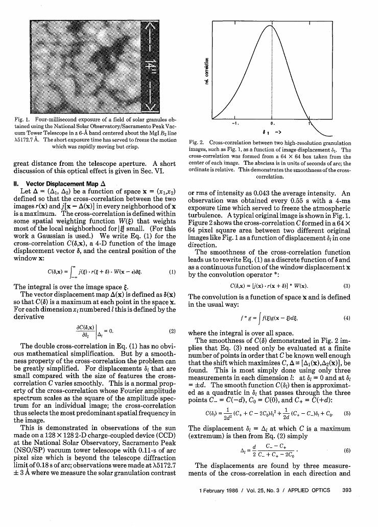
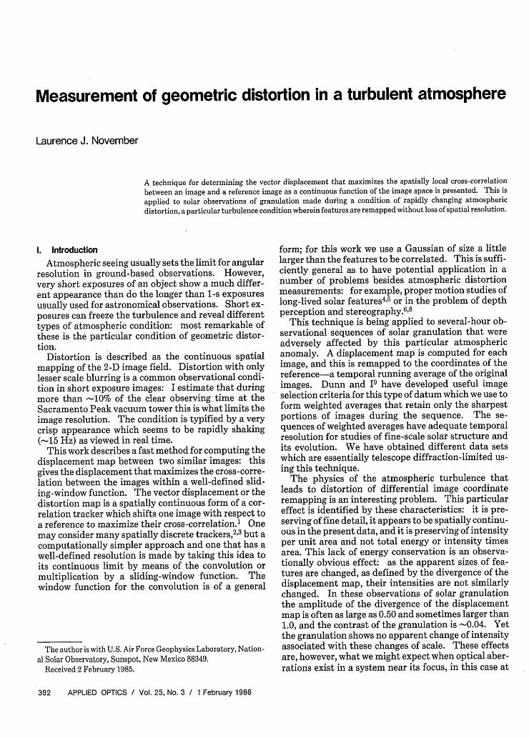
Fig. 1. Four-millisecond exposure of a field of solar granules ob-tained using the National Solar Observatory/Sacramento Peak Vac-uum Tower Telescope in a 6-A band centered about the MgI B2 lineX5172.7 A. The short exposure time has served to freeze the motion

which was rapidly moving but crisp.

great distance from the telescope aperture. A shortdiscussion of this optical effect is given in Sec. VI.

II. Vector Displacement Map ALet A = (A1 , A2) be a function of space x = (,x 2 )

defined so that the cross-correlation between the twoimages r(k) andj[k - A(k)] in every neighborhood of kis a maximum. The cross-correlation is defined withinsome spatial weighting function W(Q) that weightsmost of the local neighborhood for I j small. (For thiswork a Gaussian is used.) We write Eq. (1) for thecross-correlation C(6,x), a 4-D function of the imagedisplacement vector 6, and the central position of thewindow x:

C(b,x) J j(Q) r(Q + ) W(x - e)O9. (1)

The integral is over the image space .The vector displacement map A(x) is defined as 6(x)

so that C(6) is a maximum at each point in the space x.For each dimension xl numbered I this is defined by thederivative

IC(bx) == 0.

(2)

The double cross-correlation in Eq. (1) has no obvi-ous mathematical simplification. But by a smooth-ness property of the cross-correlation the problem canbe greatly simplified. For displacements that aresmall compared with the size of features the cross-correlation C varies smoothly. This is a normal prop-erty of the cross-correlation whose Fourier amplitudespectrum scales as the square of the amplitude spec-trum for an individual image; the cross-correlationthus selects the most predominant spatial frequency inthe image.

This is demonstrated in observations of the sunmade on a 128 X 128 2-D charge-coupled device (CCD)at the National Solar Observatory, Sacramento Peak(NSO/SP) vacuum tower telescope with 0.11-s of arcpixel size which is beyond the telescope diffractionlimit of 0.18 s of arc; observations were made at X5172.7i 3 A where we measure the solar granulation contrast

Fig. 2. Cross-correlation between two high-resolution granulationimages, such as Fig. 1, as a function of image displacement 61. Thecross-correlation was formed from a 64 X 64 box taken from thecenter of each image. The abscissa is in units of seconds of arc; theordinate is relative. This demonstrates the smoothness of the cross-

correlation.

or rms of intensity as 0.043 the average intensity. Anobservation was obtained every 0.55 s with a 4-msexposure time which served to freeze the atmosphericturbulence. A typical original image is shown in Fig. 1.Figure 2 shows the cross-correlation C formed in a 64 X

64 pixel square area between two different originalimages like Fig. 1 as a function of displacement 3 in onedirection.

The smoothness of the cross-correlation functionleads us to rewrite Eq. (1) as a discrete function of 6 andas a continuous function of the window displacement xby the convolution operator *:

C(B,x) = [(x) r(x + )] * W(x). (3)

The convolution is a function of space x and is definedin the usual way:

f * g = I f(Q)g(x -)dt, (4)

where the integral is over all space.The smoothness of C(6) demonstrated in Fig. 2 im-

plies that Eq. (3) need only be evaluated at a finitenumber of points in order that C be known well enoughthat the shift which maximizes C, A [Al (x), A2( W), befound. This is most simply done using only threemeasurements in each dimension : at = 0 and at 1= d. The smooth function C(61) then is approximat-ed as a quadratic in 6i that passes through the threepoints C_ = C(-d), Co = C(O), and C+ = C(+d):

C(01) = 1

2 (C+ + C - 2CO)61 2 + (C+-C )5 + C (5)

The displacement 6 = A1 l at which C is a maximum(extremum) is then from Eq. (2) simply

d C_-C+A 2 C_ + C+ - 2C,

(6)

The displacements are found by three measure-ments of the cross-correlation in each direction and

1 February 1986 / Vol. 25, No. 3 / APPLIED OPTICS 393

continuously in space via the convolution with thewindow W from Eq. (3).

I1. Implementation

The convolution as defined by Eq. (4) obeys thetheorem

5 * g] = YI f]- * g[g], (7)

where the Fourier transform 9A of a function of x is afunction of the wave number of x, k:

I:f(X)] J f(x) exp(*ik . x)dx,

and the Fourier transform obeys the simple inverserule f = fJ]]. For this work the cross-correlationwas computed as defined in Eq. (7) using standardcomputational fast Fourier transform methods withthe average subtracted and an apodization applied.The exact Blackman window10 applied in the imageboundary 0.04 of the overall dimension was found to beadequate to eliminate ringing. In some circumstancesthe direct computation of the integral (4) is found to befaster. This is the case for a small width Gaussianbecause the Gaussian window is dimensionally separa-ble, i.e., exp[-(x2 + y2)/g2] exp(-x2/g2 ) -exp(-y2 /g2 ).

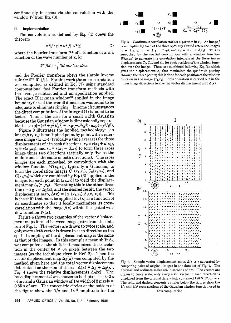
Figure 3 illustrates the implied methodology: animage (x1,x2 ) is multiplied point by point with a refer-ence image r(xl,x2 ) (typically a time average) for threedisplacements of r in each direction: r+ r(xl + d,x2 ),ro =_ r(xl,x 2 ), and r. - r(xl - d,x2) to form three crossimage times two directions (actually only five as themiddle one is the same in both directions). The crossimages are each smoothed by convolution with thewindow function W(xl,x2 ), typically a Gaussian, toform the correlation images C+(xl,x2), CO(xl,x2), andC(x1,x2 ) which are combined by Eq. (6) [applied to theimages for each point in (xl,x2 )] to yield the displace-ment map A1(x1,x2). Repeating this in the other direc-tion I = 2 gives ZA2(x), and the desired result, the vectordisplacement map, A(x) = [A(x1,x2)4 2(xbx2)]. Thisis the shift that must be applied to r(x) as a function ofits coordinates so that it locally maximizes its cross-correlation with the image j(x) within the spatial win-dow function W(x).

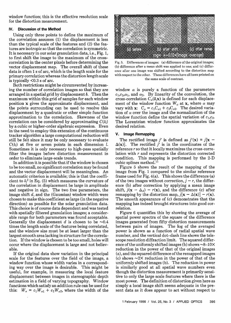
Figure 4 shows two examples of the vector displace-ment maps formed between image pairs from the datarun of Fig. 1. The vectors are drawn to twice scale, andonly every sixth vector is drawn in each direction as thespatial sampling of the displacement map is the sameas that of the images. In this example a mean shift AA

was computed as the shift that maximized the correla-tion in the center 64 X 64 pixels between the twoimages (as the technique given in Ref. 2). Then thevector displacement map AB(x) was computed by themethod given here and the total vector displacementdetermined as the sum of these: A(x) A + AB(x);Fig. 4 shows the relative displacements AB(x). Thebase displacement d was chosen to be 4 pixels - 0.42 sof arc and a Gaussian window of lie width of 8 pixels =0.85 s of arc. The concentric circles at the bottom ofthe figure show the Ile and l/e2 amplitude for the

'UM. roE

C .

-> CON

r+.U (j r)*W C+ r-|.UR

& lc_ - .

c_ + C+- 2CO

Fig. 3. Continuous correlation tracker algorithm in x1 . An imagejis multiplied by each of the three spatially shifted reference imagesro = r(xlX2), r = r(x - d, 2), and r = r(xl + d,x2). This issmoothed by the spatial convolution with a window functionW(x1,x2) to generate the correlation integrals at the three imagedisplacements CO, C_, and C+ for each position of the window func-tion over the image. These are combined following Eq. (6) whichgives the displacement A1 that maximizes the quadratic passingthrough the three points; this is done for each position of the windowfunction in the image (x1,x2). This operation is carried out in the

two image directions to give the vector displacement map A(x).

(a)14.

12.

10.

IA 8.

6.

4.

2 .

(b)14.

12.

o0.

A

x11

8.

6.

4.

2.

0.

Kv ' X ->

- / S *. 'S X 1 I / / 1 / / / fo/

,,' ' ., .. _55 _ _ ' / /-

to//,,5 5 5 I 555 /,/,.'../

t o/ ' ' ' * * * ' ' ' 5 5 5 55'

t o / 1 5 5 5 | *. 5 5 5 5 / / V / /

5. 0.

X I ->

Fig. 4. Sample vector displacement maps A(x1 ,x2) generated bycomparing pairs of original images in the data set of Fig. 1. Theabscissa and ordinate scales are in seconds of arc. The vectors aredrawn to twice scale; only every siicth vector in each direction isdisplayed from the original data which contained 128 X 128 pixels.The solid and dashed concentric circles below the figures show thelie and le 2 cross sections of the Gaussian window function used in

this computation.


II15!51\'l1I Ill 11111-fI I I I \ I I \ 1 I I I I I I I I I .

It//5'5''-- 8155l

I/ / //ll II. S S I I sXll

III/////l I I I S I II ISI

a .

A.

window function; this is the effective resolution scalefor the distortion measurement.

IV. Discussion of the Method

Using only three points to define the maximum ofthe correlation assumes (1) the displacement is lessthan the typical scale of the features and (2) the fea-tures are isotropic so that the correlation is symmetric.It is necessary in our solar granulation data, i.e., Fig. 1,to first shift the image to the maximum of the cross-correlation in the center pixels before determining thevector displacement map. The overall shift of thesedata is often 1 s of arc, which is the length scale for theprimary correlation whereas the distortion length scaleis typically <0.3 s of arc.

Both restrictions might be circumvented by increas-ing the number of correlation images so that they arearranged in a spatial grid by displacement &. Then themaximum within this grid of samples for each windowposition x gives the approximate displacement, andthe points surrounding can be used to resolve thisdisplacement by a quadratic or other simple functionapproximation to the correlation. Skewness of thecorrelation can be considered by approximating C(61)by a cubic or higher-order algebraic expression. Evenin the need to employ this extension of the continuoustracker algorithm a large computational reduction willstill be felt since it may be only necessary to evaluateC(51) at five or seven points in each dimension 1.Sometimes it is only necessary to high-pass spatiallyfilter the images before distortion measurement inorder to eliminate large-scale trends.

In addition it is possible that if the window is chosento be too small, no significant correlation may be foundand the vector displacement will be meaningless. Anautomatic criterion is available; this is that the coeffi-cient to 512 in Eq. (5) which measures the curvature ofthe correlation in displacement be large in amplitudeand negative in sign. The two free parameters, theimage shift d, and the (Gaussian) window width werechosen to make this coefficient as large (in the negativedirection) as possible for the solar granulation data.This choice is of course data dependent and was testedwith spatially filtered granulation images; a consider-able range for both parameters was found acceptable.Generally the displacement d is chosen to be .0.4times the length scale of the features being correlated,and the window size must be at least larger than thelargest smooth area lacking in structure for the correla-tion. If the window is chosen to be too small, holes willoccur where the displacement is large and not believ-able.

If the original data show variation in the principalscale for the features over the field of the image, awindow function whose width varies in a correspond-ing way over the image is desirable. This might beuseful, for example, in measuring the local featuredisplacement between images in stereographic depthestimation in a field of varying topography. Windowfunctions which satisfy an addition rule can be used forthis: W = CWal + 2 Wa2, where the width of the

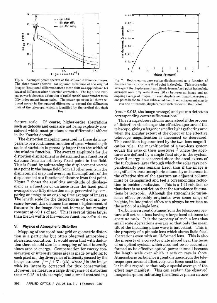
Fig. 5. Differences of images: (a) difference of the original images;(b) difference after a mean shift was applied to one; and (c) differ-ence after one image was shifted according to the distortion mapwith respect to the other. These differences have all been printed on

the same scale of contrast.

window a is purely a function of the parametersc1,c2,aj, and a2. By linearity of the convolution, thecross-correlation Ca(bx) is defined for each displace-ment of the window function Wa at x, where a mayvary with x: Ca = CICal + c2Ca2. The desired varia-tion of a over the image and the normalization of thewindow function define the spatial variation of c1,c2.The Lorentzian window function approximates thedesired relation.

V. Image Remapping

The rectified image j' is defined as j'(x) [x -A(x)]. The rectified f' is in the coordinates of thereference r so that it locally maximizes the cross-corre-lation with r and represents the distortion correctedcondition. This mapping is performed by the 2-Dcubic splines method. 1"

Figure 5 shows the result of the mapping of theimage from Fig. 1 compared to the similar referenceframe used for Fig. 4(a). This shows the difference (a)of the two images without correction, j- r, the differ-ence (b) after correction by applying a mean imageshift, (x - AA) - r(x), and the difference (c) afterremapping by the distortion map, j[x - A(x)] - r(x).The smooth appearance of (c) demonstrates that themapping has indeed brought structures into good cor-relation.

Figure 6 quantifies this by showing the average ofspatial power spectra of the square of the differenceimages generated from fifty distortion measurementsbetween pairs of images. The log of the averagedpower is shown as a function of radial spatial wavenumber, and the vertical dot-dash line shows the tele-scope resolution diffraction limit. The squared differ-ence of the uniformly shifted images (b) shows -8-10Xreduction in the power of that of the original images(a), and the squared difference of the remapped images(c) shows -2X reduction in the power of that of theuniformly shifted images (b). The reduction in poweris similarly good at all spatial wave numbers eventhough the distortion measurement is primarily sensi-tive to only the large scale features where there is themost power. The definition of distortion given here assimply a local image shift seems adequate in the pre-sent data as it does appear to act without respect to


14.

13.

e t2.

o it.0

10.

9.

0. 20.10. 1k (arcseconds )

Fig. 6. Averaged power spectra of the squared difference images.The three power spectra: (a) squared difference of the originalimages; (b) squared difference after a mean shift was applied; and (c)squared difference after distortion correction. The log of the aver-age power is shown as a function of radial spatial wave number fromfifty independent image pairs. The power spectrum (c) shows re-duced power in the squared difference to beyond the diffractionlimit of the telescope, which is identified by the vertical dot-dash

line.

feature scale. Of coarse, higher-order aberrationssuch as defocus and coma are not being explicitly con-sidered which must produce some differential effectsin the Fourier domain.

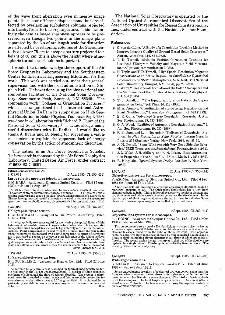
The distortion mapping measured in these data ap-pears to be a continuous function of space whose lengthscale of variation is generally larger than the width ofthe window function. The average amplitude for thedistortion displacement is determined as a function ofdistance from an arbitrary fixed point in the field.This is found by subtracting the displacement vectorat a point in the image field from all other points in thedisplacement map and averaging the amplitude of thedisplacement as a function of distance from that point.Figure 7 shows the resulting amplitude of displace-ment as a function of distance from the fixed pointaveraged over fifty distortion maps generated by com-paring an image to an ongoing time average of images.The length scale for the distortion is 3 s of arc, be-cause beyond this distance the mean displacement offeatures in the image does not increase but remainsconstant at -0.1 s of arc. This is several times largerthan the le width of the window function, 0.85 s of arc.

VI. Physics of Atmospheric Distortion

Mapping of the coordinate grid or geometric distor-tion is a particular but often observed atmosphericaberration condition. It would seem that with distor-tion there should also be a mapping of total intensitytimes area or energy. Compensation for energy con-servation or intensity times area is made by adding toeach pixel in j the divergence of intensity caused by theimage stretch: j = j + V (), where j is the imagewith its intensity corrected for flux conservation.However, we measure a large divergence of distortion(rms = 0.25 in this example) and a small contrast in

0.14

0. 12

1 0.1I_t0. 08

0.06

0. 04

0.02

0.0. 2. 4. 6. 8.

distance (arcseconds)

Fig. 7. Root-mean-square seeing displacement as a function ofdistance from an arbitrary fixed point in the field. This is the radialaverage of the displacement amplitude from a fixed point in the fieldaveraged over fifty realizations (26 s) between an image and anongoing average of images. In each displacement map the vector atone point in the field was subtracted from the displacement map to

give the differential displacement with respect to that point.

(rms = 0.043, the image average) and yet can detect nocorresponding contrast fluctuations!

This strange observation is understood if the processof distortion also changes the effective aperture of thetelescope, giving a larger or smaller light gathering areawhen the angular extent of the object or the effectivetelescope magnification is increased or decreased.This condition is guaranteed by the two-lens magnifi-cation rule: the magnification of a two-lens systemequals the ratio of their apertures,'2 where the aper-tures are defined by a single field stop in the system.Overall energy is conserved since the areal extent ofthe turbulence layer through which the solar rays per-pendicularly pass remains fixed; thus if the image ismagnified in one atmospheric column by an increase inthe effective size of the aperture an adjacent columnmust be demagnified and feel a corresponding reduc-tion in incident radiation. This is a 1-D solution sothat there is no restriction that the turbulence fluctua-tions be isotropic. Although the atmospheric turbu-lence effect probably originates over some range ofheights, its integrated effect can always be written asthe action of a single lens.

Turbulence a great distance from the telescope aper-ture will act as a lens having a large focal distance toaperture ratio. It is the property of such a lens thatsmall scale aberrations average so that only the meantilt of the incoming plane wave is important. This isthe property of a pinhole lens which shows little focalaberrations even with an ill-formed lens. This is alsothe property of a corrector plate placed near the focusof an optical system, which need not be so accuratelyformed as its effective optical power is small becausethe length scale over which it acts on rays is short.Atmospheric turbulence a great distance from the tele-scope aperture and effectively near focus must be simi-lar in this regard, so that only a spatial average of theeffect may manifest. This can explain the observedimage sharpness indicating the effective planar nature


5' --- (a) before(b) after shift

- (c) after remap

-- -

of the wave front aberration even in nearby imagepoints that show different displacements but are af-fected by overlapping turbulence columns projectedinto the sky from the telescope aperture. This is seem-ingly the case as image sharpness appears to be pre-served even though two points in the image planeseparated by the 3-s of arc length scale for distortionare affected by overlapping columns of the Sacramen-to Peak tower 75-cm telescope aperture projected to aheight of 50 km; this is above the height where atmo-spheric turbulence should be important.

I would like to acknowledge the support of the AirForce Geophysics Laboratory and the SoutheasternCenter for Electrical Engineering Education for thiswork. This work was carried out under their generalsupervision and with the local administration of Ste-phen Keil. This was done using the observational andcomputing facilities of the National Solar Observa-tory, Sacramento Peak, Sunspot, NM 88349. Thecompanion work "Collages of Granulation Pictures,"which is now published in the International Astro-physical Union (IAU) in its symposium on High Spa-tial Resolution in Solar Physics, Toulouse, Sept. 1984was done in collaboration with Richard B. Dunn of theNational Solar Observatory. 9 I acknowledge manyuseful discussions with R. Radick. I would like tothank J. Evans and D. Neidig for suggesting a viablemechanism to explain the apparent lack of energyconservation by the action of atmospheric distortion.

The author is an Air Force Geophysics Scholar.This research is sponsored by the Air Force GeophysicsLaboratory, United States Air Force, under contractF19628-83-C-0097.

The National Solar Observatory is operated by theNational Optical Astronomical Observatories of theAssociation of Universities for Research in Astronomy,Inc., under contract with the National Science Foun-dation.

References

1. 0. von der Ltihe, "A Study of a Correlation Tracking Method toImprove Imaging Quality of Ground-Based Solar Telescopes,"Astron. Astrophys. 119,85 (1983).

2. T. D. Tarbell, "Multiple Position Correlation Tracking forLockheed Filtergram Velocity and Magnetic Field Measure-ments," private communication (1982).

3. K. Topka and T. D. Tarbell, "High Spatial Resolution MagneticObservations of an Active Region," in Small-Scale DynamicalProcesses in the Stellar Atmospheres, X. X. Keil, Ed. (NationalSolar Observatory, Sunspot, NM, 1984), pp. 278-286.

4. F. Ward, "The General Circulation of the Solar Atmosphere andthe Maintenance of the Equatorial Acceleration," Astrophys. J.141, 534 (1965).

5. T. L. Duvall, Jr., "The Equatorial Rotation Rate of the Super-granulation Cells," Sol. Phys. 64, 213 (1980).

6. M. A. Crombie, "Coordination of Stereo Image Registration andPixel Classification," J. Am. Soc. Photogramm. 49, 529 (1983).

7. B. K. Opitz, "Advanced Stereo Correlation Research," J. Am.Soc. Photogramm. 49, 533 (1983).

8. G. A. Wood, "Realities of Automatic Correlation Problems," J.Am. Soc. Photogramm. 49, 537 (1983).

9. R. B. Dunn and L. J. November, "Collages of Granulation Pic-tures," in High Resolution in Solar Physics, Lecture Notes inPhysics 233 (Springer-Verlag, New York, 1985, pp. 85-90.

10. A. H. Nuttall, "Some Windows with Very Good Sidelobe Beha-vior," IEEE Trans. Acoust. Speech Signal Process. 29,84 (1981).

11. J. L. Walsh, J. H. Ahlberg, and E. N. Nilsen, "Best Approxima-tionProperties of the Spline Fit," J Math. Mech. 11,225 (1962).

12. R. Kingslake, Optical System Design (Academic, New York,1983).

Patents continued from page 3864,534,626 13 Aug. 1985 (Cl. 350-454)Large relative aperture telephoto lens system.S. MIHARA. Assigned to Olympus Optical Co., Ltd. Filed 17 Aug.1983 (in Japan 24 Aug. 1982).

An f/2 telephoto objective is described for use at a focal length of -250 mm.The system contains eleven elements in four groups (+ - -: +), groups 2 and 3moving backward and group 4 moving forward when focusing on a near object.Glasses having unusual partial dispersion are used to reduce the secondaryspectrum. Four embodiments are given controlled by ten conditions. R.K.

4,536,086 20 Aug. 1985 (Cl. 356-348)Holographic figure sensor.D. M. SHEMWELL. Assigned to The Perkin-Elmer Corp. Filed18 Nov. 1982.

A holographic figure sensor useful for monitoring the optical figure of thinlightweight deformable mirrors of large aperture is described. It incorporatessubaperture sized zone plates that are holographically recorded on the mirrorsurface. Point source images formed by light diffracted from the zone plateswhen the mirror is illuminated by a point source near its center of curvatureare in turn used to generate a corrector plate hologram of the mirror surface.Wave fronts reconstructed from this hologram by the zone plate images duringsystem operation are interfered with a reference beam to create an interfero-gram that allows surface errors across the mirror aperture to be recovered.

David Thomas for B.J.H.

4,537,464 27 Aug. 1985 (Cl. 350-1.4)Infrared objective system lens.R. BOUTELLIER. Assigned to Kern & Co., Ltd. Filed 22 June1983.

An infrared f/i objective lens is described for thermal imaging with moder-ate resolution in the 3.5-5.0-)um spectral band. It consists of three elements,two being of silicon and the third of calcium fluoride. The system is achro-matic over its intended spectral range and has reasonable correction formonochromatic aberrations over a 3.2° angular field. It is claimed to beparticularly suitable for use with a scanning mirror between the lens anddetector. R.A.

4,537,472 27 Aug. 1985 (Cl. 350-414)Objective lens system for microscopes.Y. ASOMA. Assigned to Olympus Optical Co., Ltd. Filed 6 Feb.1984 (in Japan 15 Feb. 1983).

A 60X flat-field oil-immersion microscope objective is described having anumerical aperture of 1.4. The thick front hemisphere has a tiny frontelement embedded in it. This is followed by a positive meniscus element andtwo thick cemented triplets, each of which contains a fluorite element. In therear is a pair of thick negative doublets similar to those in a double Gaussobjective. Two examples are given controlled by six conditions. R.K.

4,540,248 10 Sept. 1985 (Cl. 350-414)Objective lens system for microscopes.T. TOGINO. Assigned to Olympus Optical Co., Ltd. Filed 5 Mar.1984 (in Japan 24 Mar. 1983).

Two embodiments are given of a 5OX flat-field microscope objective havinga numerical aperture of 0.55 to be used in combination with a particular three-element telescope objective in the tube of the microscope. The objectivecontains a positive front meniscus followed by four cemented doublets and anegative doublet, making eleven elements in all, three of which are made offluorite. The second design is slightly simpler in that two of the doublets arereplaced by a single triplet. The design is controlled by five conditions. Theworking distance is unusually long. R.K.

4,540,249 10 Sept. 1985 (Cl. 350-426)Wide angle zoom lens.S. MOGAMI. Assigned to Nippon Kogaku K.K. Filed 24 June1982 (in Japan 3 July 1981).

Seven embodiments are given of a classical two-component zoom lens, thefront negative component having three or four elements, while the positiverare component has five, six, or seven elements. The third surface is asphericin all the examples. The focal length range is from 21 to 35 mm at f/3.5 or21-40 mm at f/3.5-4.5. The lens element carrying the aspheric surface ismade of plastic material. R.K.


Documents

Measurement Of Geometric Distortion In A Turbulent Atmosphere