Embed Size (px)
Citation preview

Measurement of the Remanent Magnetization of Igneous Rocks
GEOLOGICAL SURVEY BULLETIN 1203-A


Measurement of the Remanent Magnetization of Igneous RocksBy RICHARD R. DOELL and ALLAN COX
EXPERIMENTAL AND THEORETICAL GEOPHYSICS
GEOLOGICAL SURVEY BULLETIN 1203-A
An induction magnetometer, a portable drill, and a computer program
UNITED STATES GOVERNMENT PRINTING OFFICE, WASHINGTON : 1965

UNITED STATES DEPARTMENT OF THE INTERIOR
STEWART L. UDALL, Secretary
GEOLOGICAL SURVEY
Thomas B. Nolan, Director
The U. S. Geological Survey Library has cataloged this publication as follows:
Doell, Richard Rayman, 1923-Measurement of the remanent magnetization of igneous
rocks, by Richard R. Doell and Allan Cox. Washington, U. S. Govt. Print. Off., 1965.
iv, 32 p. illus., diagrs., table. 24 cm. (U. S. Geological Survey. Bulletin 1208-A)
Theoretical and experimental geophysics. Bibliography: p. 32.
1. Rocks, Igneous. 2. Magnetism, Terrestrial. 3. Magnetometer. 4. Electronic data processing-Magnetometer. I. Cox Allan V 1926- joint author. II. Title. (Series)
For sale by the Superintendent of Documents, U.S. Government Printing Office Washington, D.C. 20402 - Price 20 cents (paper cover)
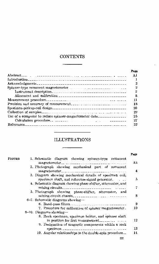
CONTENTS
Abstract__ _______________________________________Introduction _______________________________________Acknowledgments. _________________________________Spinner-type remanent magnetometer_________________
Instrument description._________________________Alinement and calibration.______________________
Measurement procedure.____________________________Precision and accuracy of measurement.______________Specimen-pickup-coil design__________________________Collection of samples________________________________Use of a computer to reduce spinner-magnetometer data-
Calculation procedure.. _ ________________________References. ________________________________________
Page Al
12228
11182022252732
ILLUSTRATIONS
showing spinner -type remanent ______________________________mechanical part of remanent
FIGURE 1. Schematic diagram magnetometer ______
2. Photograph showingmagnetom eter _ ___________________________________
3. Diagram showing mechanical details of specimen coil, specimen shaft, and reference-signal generator________
4. Schematic diagram showing phase shifter, attenuator, and mixing circuits. __________________________________
5. Photograph showing phase-shifter, attenuator, and mixing-circuit chassis. _-__________-______-_---____
6-7. Schematic diagrams showing 6. Band-pass filters- _ __________________-_-_-_-_---7. Procedure for calibration of spinner magnetometer.
8-10. Diagrams showing 8. Rock specimen, specimen holder, and spinner shaft
in position for first measurement... ___-_____--_9. Designation of magnetic components within a rock
specimen.. . __ _ ______________________________10. Angular relationships in the double-spin procedure..
ni
Page
A3
910
12
1314
IV CONTENTS
Page FIGURE 11-12. Graphical calculations showing
11. Direction of remanent magnetization within aspecimen from spinner-magnetometer data_ _ ___ A16
12. In-place direction of remanent magnetization from orientation data and specimen-magnetization- direction data.-_____-_______-_-_-___-___-__ 17
13-14. Diagrams showing 13. Relations of position of pickup coil to rotating
specimen__ _______________________________ 2014. Curves of equal incremental signal-to-noise ratio__ 22
15. Photograph showing sample-coring drill with water tankand orienting devices_____--_--_--__-_--_---___--__ 23
16-17. Diagrams showing 16. Mechanical details of the core-drill transmission. _ 2317. Declination gradiometer.______________________ 25
TABLE
Page TABLE 1. Specimen orientations for six spins._____-_-__-__--_-____-__ A14

EXPERIMENTAL AND THEORETICAL GEOPHYSICS
MEASUREMENT OF THE REMANENT MAGNETIZATION OF IGNEOUS ROCKS
By RICHARD R. DOELL and ALLAN Cox
ABSTRACT
The design of a simple motor-driven spinner magnetometer for measuring remanent magnetization in the range 1X10~S to 1.0 emu per cc (electromagnetic units per cubic centimeter) is presented; included are practical details of mechani cal components and electronic circuits and procedures of operation and calibration. In routine use over a 2-year period, two of these instruments have measured directions of remanent magnetization of rock specimens with an estimated ac curacy of 1 ° and have measured intensities with an estimated accuracy of several percent; they have required infrequent calibration and only minor maintenance. Computational techniques are given for calculating magnetic moments and direc tions from magnetometer-output data using either graphical procedures or numerical methods suitable for machine calculation. The design of a light weight portable drill for coring samples in place and procedures for accurately orienting cores using a mechanical stage are also given.
INTRODUCTION
Most igneous rocks have natural remanent magnetizations in the range 10~4 to 10~ 2 emu per cc (electromagnetic units per cubic centi meter), although intensities as high as several such units may occur near areas where lightning bolts have struck (Cox, 1961; Graham, 1961). For paleomagnetic research on igneous rocks, an instrument with a sensitivity somewhat greater than 10~4 emu per cc is generally needed to measure the remanent magnetization of rock specimens after they have been partially demagnetized. This report describes a spinner-type magnetometer suitable for magnetic analysis of most igneous rocks. It is capable of accurately measuring remanent magnetizations in the range 1X 10~5 to 1.0 emu per cc with an ultimate sensitivity of 10~6 emu per cc. Long-term stability, measurement accuracy, and efficiency of operation, rather than high sensitivity, were primary considerations in the design of this instrument, which is a variation of instruments previously described by Johnson and McNish (1938) and by Nagata (1961, p. 58-64).
Al

A2 EXPERIMENTAL AND THEORETICAL GEOPHYSICS
ACKNOWLEDGMENTS
We wish to thank Major Lillard for construction of the spinner magnetometers, field core drills, and associated equipment; we are indebted also to Thomas Robinson and Edward Roth for assistance with the measurements used for analyzing the operation of the spinner magnetometers.
SPINNER-TYPE REMANENT MAGNETOMETER
INSTRUMENT DESCRIPTION
The general arrangement of the apparatus is depicted in figure 1. A nonmagnetic shaft, rotated at 109 cps (cycles per second) (6,540 rpm) by an induction-type electric motor, is fitted with a specimen holder at one end and reference magnets at the other. The specimen and reference magnets thus induce signals of the same frequency in their respective pickup coils. The signal from the reference coils passes first through a phase shifter which shifts the output phase at angles from 0° to 360° with respect to the input-phase angle; the signal then passes through a voltage attenuator which varies the reference-signal amplitude over a range of 1X 10~ 6 to 1.0. The output signal from the reference attenuator is added to the signal from the specimen pickup coil in a mixing circuit, and the sum is amplified, filtered, and displayed on a cathode-ray oscilloscope.
The reference-signal phase shifter and attenuator are so calibrated than when the two signals entering the mixing circuit total zero, the direction of the specimen's magnetic moment projected normal to the shaft axis is read directly from the phase-shifter dial, and the intensity of this moment, in electromagnetic units, is read from the attenuator dials.
Because the signal coil, reference coils, phase shifter, attenuator, and mixing circuits are all passive networks, they are not subject to electronic drift and therefore do not need repeated calibration. Changes in the electronic circuits of the amplifier, filters, and cathode- ray oscilloscope affect only the ease with which null signals can be read; they do not affect calibration.
Figure 2 is a photograph of the mechanical parts of the apparatus, and figure 3 shows a detailed drawing of the signal-generating part of the unit. The specimen, a cylinder 2.49 cm in diameter by 2.28 cm long, is clamped in a cubical holder of clear plastic, which in turn fits into a square indentation at one end of the shaft (fig. 8). The other end of the shaft, which is constructed from laminated phenolic material, supports two disk-shaped permanent magnets that have been magnetized in opposite directions along their diameters. The shaft rotates in two bronze bushings mounted in a brass bearing

Belt
6540
rpm
d
l"iv
e
x^s
345V
rp
m
V.
Drive
m
oto
r
Refe
rence
m
ag
ne
ts
Sig
na
l co
ilP
ha
se
sh
ifte
rA
ttenuato
r
Mix
ing
circu
itA
mplif
ier
Band-p
ass
filte
rC
ath
od
e-r
ay
osc
illosc
ope
FIG
URE
1
. S
pin
ner
-ty
pe
rem
anen
t m
agne
tom
eter
.

A4 EXPERIMENTAL AND THEORETICAL GEOPHYSICS
FIGURE 2. Mechanical part of remanent magnetometer.
support and is driven by a K-horsepower induction-type electric motor through a 2-meter-long shaft and a V-belt drive. The motor is sufficiently powerful to operate within 1 percent of its rated speed under all normal load and powerline variations and is far enough removed from the pickup coils not to induce unwanted signals in the detecting units.
The specimen pickup coil is of the balanced type, that is, the outer windings are in opposition to the inner windings and are so chosen that the net flux linkage from uniform magnetic fields through the two coils is zero. The rationale for the shape of the windings is described on page A20. On our instrument, the inner winding contains 1,800 turns of 26 AWG copper transformer wire, and the outer windings have 187 turns of 24 wire. The coil impedance at 109 cps is 87 ohms. The entire pickup coil is covered by an elec trostatic shield constructed of thin aluminum strips, so arranged as to form no large current loops.
Because the unknown specimen signal in a magnetometer of this type is determined by comparison with a known reference signal (Bruckshaw and Robertson, 1948), the measurement accuracy is strictly limited by the stability and accuracy of the reference-signal system. Ideally, the reference-signal phase angles should be exactly equal to the angular position of the dial which indicates the magnetic direction, and the output of the attenuator should be exactly pro-

E
FIG
UR
E 3.
Mec
han
ical
de
tail
s of
sp
ecim
en
coil,
sp
ecim
en
shaf
t, an
d re
fere
nce-
sign
al g
ener
ator
(s
how
n ab
out
one-
half
siz
e).
A,
Spec
imen
; B
, sp
ecim
en h
olde
r; C
, sh
aft;
D,
shaf
t be
arin
gs;
E,
lubr
icat
ion
fitt
ings
; F
, be
arin
g su
ppor
t; G
, dr
ive
pull
ey;
H,
refe
renc
e m
agne
ts;
/, r
efer
ence
-coi
l co
res;
J,
refe
renc
e-ge
nera
tor
supp
ort;
K,
mai
n pi
ckup
coi
l; L,
bal
anci
ng c
oil.
1 §
A6 EXPERIMENTAL AND THEORETICAL GEOPHYSICS
portional to the position of the dial which indicates magnetic moment. The phase shifter and attenuator should also function independently, and it is convenient if the reference signal is large enough to measure strong magnetic moments directly without attenuation of the signal from the specimen pickup coil.
In our instrument a large three-phase reference signal is generated by rotating 2 disk-shaped magnets, 19 mm in diameter by 1.25 mm thick, near 12 stationary pickup coils. Because the magnets have rather large moments, they are alined in opposite directions and carefully astaticized to produce no detectable signal in the specimen pickup coil. (See p. A8.) The reference coils are placed at 60° intervals about the two reference magnets, and each coil contains 1,500 turns of 44 AWG copper transformer wire wound on a soft iron core. Three groups of four coils, each with the same phase angle, are connected in series fashion, and at 109 cps each group has an impedance of about 280 ohms. The position of each coil can be adjusted radially to balance the three-phase signal during the aline- ment and calibration procedure.
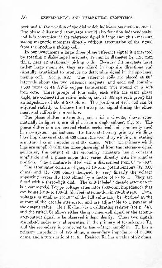
The phase shifter, attenuator, and mixing circuits, shown sche matically in figure 4, are all placed in a single cabinet (fig. 5). The phase shifter is a commercial electromechanical unit commonly used in servosystem applications. Its three stationary primary windings have impedances of about 300 ohms; the secondary winding, a rotating armature, has an impedance of 500 ohms. When the primary wind ings are supplied with the three-phase signal from the reference-signal generator, the output of the secondary armature has a constant amplitude and a phase angle that varies directly with its angular position. The armature is fitted with a dial scribed from 0° to 360°.
The attenuator consists of ganged 10-turn potentiometers K2 (500 ohms) and K3 (300 ohms) designed to vary linearly the voltage appearing across K5 (550 ohms) by a factor of %o to 1. They are fitted with a three-digit dial. The unit labeled "decade attenuator" is a commercial T-type voltage attenuator (600-ohm impedance) that can be set for 0- to 100-db (decibel) attenuation in 20-db steps. Thus, voltages as small as 1X 10~6 of the full value may be obtained at the output of the decade attenuator and are adjustable to 1 percent of the output value. K4 (5K ohms) is a calibrating resistor (see p. As), and the switch SI allows either the specimen-coil signal or the attenu ator-output signal to be observed independently. These two signals are mixed under normal operation in the primary of transformer Tl, and the secondary is connected to the voltage amplifier. Tl has a primary impedance of 125 ohms, a secondary impedance of 39,000 ohms, and a turns ratio of 1:18. Resistor Rl has a value of 22 ohms.
Fro
m
1 \
refe
ren
ce
coils
_
\ I
FIG
URE
4. P
has
e sh
ifte
r, a
tten
uato
r, a
nd m
ixin
g ci
rcui
ts.
C^ «_
Fro
m
SI
I \
sp
ecim
en
1
I -
coil
§ « § CO o O w co

A8 EXPERIMENTAL AND THEORETICAL GEOPHYSICS
FIGURE 5. Phase-shifter, attenuator, and mixing-circuit chassis.
The amplifier is a commercial unit with low input noise level and adjustable gain from 0 to 85 db. Its input impedance is about 1 megohm, and the output impedance is 3,000 ohms. A schematic drawing of the band-pass filters, which are the electronic-feedback type (Gray, 1954, p. 682-685), is shown in figure 6. The ganged potentiometers R5-R9 and R6-R10 adjust the band-pass center frequency (coarse and fine adjustment, respectively), and the resistors R13 (fine) and Rl4 (coarse) adjust the width of the pass band and the Q of the filter frequency response. The cathode-ray oscilloscope used as a null detector is a general-purpose unit that has moderate input sensitivity.
ALINEMENT AND CALIBRATION
To astaticize the reference magnets with respect to the specimen pickup coil, the inner reference magnet is magnetized to saturation along a diameter and then for stability, is partially demagnetized in an alternating field of 300-oersted peak value. The outer magnet is magnetized to saturation in the opposite sense and then partially demagnetized in steps until no signal can be observed at the highest sensitivity level of the null-detector system, as described below.

REMANENT MAGNETIZATION OF IGNEOUS ROCKS A9
R1 = 330KR2=1MR3=R4=R16=1.8KR5=R9=500K'R6=R10=R13=50K
R7=R8=R17=3.9K R11 = R15=22K R12=5.6K R14=250K R18=470K
C2=C3=0.005jiC4=40/iV1 = V2= V3= V4=K(12AX7)B+ = 135v regulated
FIGURE 6. Band-pass filters.
After the calibration adjustment resistor K4 has been roughly adjusted using either a known test magnet or the calibration circuit described below, the three signals from the reference coils are balanced. The most sensitive way of adjusting the reference coils is to observe the output of the phase shifter rather than to observe the intensity of the reference coils directly. A test magnet or rock specimen is placed in the specimen holder, measured, rotated within the holder exactly 30° about the shaft axis, and remeasured; the process is repeated for 12 measurements. The phase-dial readings and attenuator settings are then plotted against the test-magnet angles. Ideally the phase- dial reading should be a linear function of the test-magnet angle over the entire range of 0° to 360°, and the attenuator settings should be constant; by trial and error the coils are moved radially until this condition is attained. We have been able to obtain phase linearity to about 0.1° and constant amplitude to within 1 percent. After the three-phase reference signal is balanced, the phase dial may then be so placed on the shaft of the phase shifter that it reads 0° when the test specimen has its moment alined with the zero reference mark on the specimen holder.
The next step is to adjust exactly the intensity calibration resistor R4. The output of the attenuator is linear for all ranges except for the 0-db setting of the attenuator. Thus, if a specimen or test magnet is available with accurately known moment (less than 1.0 emu), the 20- to 100-db attenuation ranges of the instrument may be calibrated by setting the attenuator to the known moment of the

A10 EXPERIMENTAL AND THEORETICAL GEOPHYSICS
rpm
Magnet
Signal coil
FIGUEE 7. Procedure for calibration of spinner magnetometer.
magnet and adjusting resistor R,4 to give a null on the oscilloscope. For the rarely used 0-db attenuation range, a calibration chart must be prepared.
Standard magnetic specimens may be used to prepare this calibra tion chart and to check the linearity of the instrument. An alternative calibration method which uses an alternating-current meter as a primary standard is shown in figure 7. The specimen pickup coil is replaced by an auxiliary coil, and a magnet is rotated in the specimen holder. The signal induced in the auxiliary coil is amplified by a power amplifier and supplied to a test coil through an accurate current meter. Our test coil consists of a single layer of 39 turns of 24 AWG copper transformer wire wound on a cylindrical form 2.49 cm in diameter and 2.28 cm long (the specimen size). During the test, its axis is alined along the specimen-pickup-coil axis, and it is placed at the same distance from the pickup coil that a specimen would have during normal operation. The test coil induces a signal in the specimen pickup coil equivalent to a specimen of magnetic moment :
M (eum)=25.53i rms (amperes),
where irms is the root-mean-square current supplied to the test coil. Thus, signals equivalent to any desired specimen magnetic moment

REMANENT MAGNETIZATION OF IGNEOUS ROCKS All
may be induced in the pickup coil and nullified with the reference signal in the manner used for normal operation.
Because the filters are the feedback type, resistors R13 and R14 (fig. 6) can be so adjusted that the units go into a self-sustained oscilla tion. For optimum filtering (smallest band-pass width), Rl3 and R14 are adjusted so that the filters are just below the point where sustained oscillation occurs. Then when the spinner is running and a signal appears on the oscilloscope, the resistors R5-R9 and R6-R10 are adjusted to give a maximum signal on the oscilloscope. When so adjusted, the band-pass peak is at the operating frequency of the spinner. Unless the specimens being measured have magnetic mo ments near the minimum values measurable on these instruments, it is not necessary to use an extremely narrow pass band, and adjustments need be made only a few times each week.
During several years of operation, in which two different standard specimens were measured each week to test the operation and calibra tion of the magnetometers, it has not been necessary to change any of the adjustments described above or to change the adjustment of the calibration resistor. Although it is necessary occasionally to adjust the filter circuits to improve noise rejection, it should be noted that these adjustments do not affect the calibration.
MEASUREMENT PROCEDURE
Attenuator and phase-dial readings recorded by spinning about one axis of the specimen determine only the component of the magnetic moment normal to the axis of spinning. At least one more datum must therefore be obtained by spinning the specimen about a different axis to determine the total magnetic moment and its direction within the specimen. Several additional measurements are desirable to minimize effects of induced magnetic anisotropy and specimen in- homogeneity and to estimate the precision of a single determination of the remanent magnetism of a specimen.
In our system for obtaining oriented samples in the form of cores (described on p. A22), the specimens later cut from these samples are assigned right-handed orthogonal axes x, y, and z. The z axis is along the specimen cylinder axis, the y axis is along the specimen diameter that was horizontal in the in-place position, and the x axis is along the diameter normal to the y axis. When a specimen is placed in a speci men holder (fig. 8), each of the three axes is parallel to one of the cube edges of the holder. The square indentation in the spinner shaft is arranged so that one of the axes of the specimen is in the zero position; this direction is marked "I" on the shaft, and the direction 90° clockwise is marked "II".

A12 EXPERIMENTAL AND THEORETICAL GEOPHYSICS
After the unit is properly calibrated and the filters adjusted, a single measurement can be made by the following procedure:
1. Place the specimen holder in the shaft in the desired position and start the shaft spinning.
2. Short out the reference signal with the switch Si and adjust the amplifier gain so that a convenient signal from the specimen appears on the cathode-ray oscilloscope.
3. Leaving the amplifier gain unchanged, move switch SI to short out the signal from the specimen and adjust the attenuator until a signal of similar size from the reference magnets appears on the cathode-ray oscilloscope.
4. Move switch Si to its center position and alternately adjust the phase dial and attenuator until no signal appears on the cathode- ray oscilloscope; as the null is approached, the amplifier gain should be increased so that small adjustments of the phase dial and the attenuator away from the null settings cause easily recognizable signals to appear on the cathode-ray oscilloscope. The setting on the phase dial is the angle of the component of magnetization normal to the spin axis measured clockwise from the I mark on the shaft, and the attenuator settings record its magnetic moment in electromagnetic units. Nulls usually can be easily achieved without use of the shorting switch unless intensities vary greatly between measurements.
FIGURE 8. Rock specimen, specimen holder, and spinner shaft in position for first measurement (spin 1 in table 1).
REMANENT MAGNETIZATION OF IGNEOUS ROCKS
A-x
A13
+2 (specimen-cylinder axis)
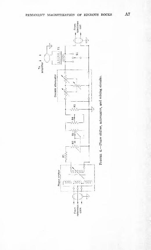
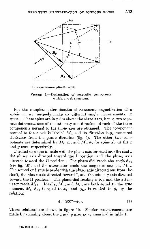
FIGURE 9. Designation of magnetic components within a rock specimen.
For the complete determination of remanent magnetization of a specimen, we routinely make six different single measurements, or spins. These spins are in pairs about the three axes, hence two sepa rate determinations of the intensity and direction of each of the three components normal to the three axes are obtained. The component normal to the z axis is labeled Mz , and its direction is <j>z , measured clockwise from the plus-x direction (fig. 9). The other two com ponents are determined by Mx, <t>x , and My, <j>v for spins about the x and y axes, respectively.
The first or a spin is made with the plus-2 axis directed into the shaft, the plus-a; axis directed toward the I position, and the plus-?/ axis directed toward the II position. The phase dial reads the angle 4> z>a (see fig. 10), and the attenuator reads the magnetic moment Mz, a . The second or b spin is made with the plus-s axis directed out from the shaft, the plus-z axis directed toward I, and the minus-?/ axis directed toward the II position. The phase-dial reading is (f>Zi B and the atten uator reads M2>6 . Ideally, Mz, a and MZi 6 are both equal to the true moment Mz ; <f> s>a is equal to <£«; and <£ a, 6 is related to (f>z by the relation:
$3=360 $2, B . (1)
These relations are shown in figure 10. Similar measurements are made by spinning about the x and y axes as summarized in table 1.
745-239 O 64 3

A14 EXPERIMENTAL AND THEORETICAL GEOPHYSICS
SPIN 1 SPIN 2
, a
FIGURE 10. Angular relationships in the double-spin procedure.
TABLE 1. Specimen orientations for six spins
Spin
1... . -.. ... .... ..234. .._... -56
Axis directed into shaft
+2 2
+z X
+y -v
Axis towards I direction
+x +x+y +y+2 +2
Axis towards II direction
+V -V+z z +x X
Data obtained
Moment
M, M2 6MX a MX 6My a
My b
Angle
©- ©- ©-«-«- ©-
Measurements about the z, x, and y axes are combined in pairs as follows:
(2a)
(2b)
Use of these averages rather than a single measurement about each axis reduces possible errors due to inhomogeneity or anisotropy in the specimen, and provides redundant data to check measurement accu racy and precision. Averaging also automatically corrects for any possible systematic error in phase-angle measurement, inasmuch as the same error angle is added to both 02 , a and <f>z, 6 , for example, and

REMANENT MAGNETIZATION OF IGNEOUS ROCKS A15
drops out in step 2b above. When the direction of the component normal to the spin axis falls near the I position, both 0g( and 02> 6 , for example, may fall on the same side of the zero-phase reading. This may be caused by small measurement errors or by the systematic errors mentioned above. When both phase angles fall on the same side of zero, the expressions (2b) should be replaced by
(2c)
t)j
The total magnetic moment is given by
(3a)
,)» (3b)
The key to finding the direction of magnetization from spinner- magnetometer measurements lies in noting that during each spin the component of magnetization parallel to the rotation axis does not contribute to the signal generated in the pickup coil. Thus the angle 02 is consistent with any vector lying in a half plane having an edge along the rotation axis and extending in the direction 02 ; the same applies for <f>x and <£ . One method of determining the direction of magnetization in a specimen uses phase angles and intensities in combination. The component of the total magnetization along the z direction is given by Mx sin 4>x My cos <j> y , and similarly for the com ponents along the x and y directions. These pairs of values may then be averaged and the direction and intensity of magnetization in the specimen calculated from these three vector components.
An alternative method using only phase angles is preferable for most purposes because phase angles can be measured with greater precision than intensities and can easily be checked for internal con sistency. As previously noted, the 0Z measurement is consistent with all vectors lying in a half plane passing through the z axis, and the 0X measurement is consistent with all vectors in a plane passing through the x axis; therefore the only vector consistent with both measurements is along the intersection of these two planes. The 4>x and <j> y measurements similarly define a unique vector consistent with both measurements, as do the <f>v and <f> z measurements. The mean of these three vectors may be taken as the direction of magne tization of the specimen, and the angular differences between the vectors as a measure of the precision of the measurement.
A graphical technique using an equal-area or stereographic projec tion has been given by Graham (1949). The planes defined by 0,,

A16 EXPERIMENTAL AND THEORETICAL GEOPHYSICS
FIGURE 11. Calculation of the direction of remanent magnetization within a specimen from spinner-magnetometer data.
<t>x, and <£ are drawn as great circles on the projection (fig. 11) and usually intersect to form a small-error triangle. The radius of the circle inscribed in this triangle is commonly used to check the pre cision, and its center, defined by the angles 0Z and ~dz , is commonly used as the best estimate of the direction of magnetization. A minor difficulty in using this method for determining the mean direction arises when the magnetization of the specimen is nearly parallel to a rotation axis. Signals which are weaker and less well defined than the others are generated by spinning about that axis, but the plane defined by these weaker spins is given nearly equal weight if the center of the inscribed circle is taken as the direction of magnetization. This factor can be qualitatively considered by taking the best estimate of the magnetic direction nearer the intersection of the two planes defined by the stronger signals. A quantitative analytical method for

REMANENT MAGNETIZATION OF IGNEOUS ROCKS A17
weighting the stronger and more reliable measurements is given on page A25.
To find the magnetic declination D and inclination / corresponding to the original orientation of the specimen, let a be the geographic azimuth of the horizontal y axis, /3, the plunge of the z axis, 4> g , the azimuth of the magnetic vector reckoned clockwise from x in the xy plane, and 0 Z, the inclination of the magnetic vector above ( ) or below (+) the xy plane, as shown in figure 12. The -\-z axis is first rotated (90 /3)° toward the -\-x axis, and the magnetic vector is rotated the same angular displacement along a small circle having the y axis as its center. The plane of projection thus becomes the horizonta plane corresponding to the original orientation of the specimen. If geographic north is marked at an angle a counterclockwise from y, then D and / may be read directly from the projection, as indicated in figure 12.
FIGURE 12. Calculation of in-place direction of remanent magnetization from orientation data and specimen-magnetization-direction data.

A18 EXPERIMENTAL AND THEORETICAL GEOPHYSICS
A program for carrying out on a digital computer all of the calcula tions described in this section, along with additional calculations designed to check the internal consistency of the phase-angle and intensity measurements is given'on page A27.
PRECISION AND ACCURACY OF MEASUREMENT
Instrumental precision was determined by making nine measure ments in succession on a specimen having an intensity of magnetization of 1.5X10" 3 emu per cc. When the specimen was removed from the holder between successive measurements, the direction of magnetiza tion could be measured with a reproducibility of 0.7° sd (standard deviation) and the intensities to 1.1 percent (Doell and Cox, 1963). When the specimen was left in the holder between successive measure ments, the reproducibility was 0.2°sd. Thus measurement precision is primarily limited by the accuracy with which specimens can be alined in the holder.
The measurement accuracy of these instruments can be conveniently separated into several parts: (1) the accuracy of the original calibra tions, (2) the rate of drift or change in this calibration with time, and (3) the amount of error introduced in the measurements by such factors as specimen shape, specimen inhomogeneity, and susceptibility anisot- ropy.
During the original alinement and calibration procedures set forth above, the reference-signal system may be adjusted so that a phase angle, corresponding to a magnetic-component direction, is determined to within ±0.1°. The accuracy of the intensity determination de pends on the linearity of the attenuator units, rated at 1 percent, and on the accuracy of the alternating-current meter used in setting the calibration resistor R4. Our meter is rated at 1 percent.
Any change in the output signal from the reference system between calibration checks will reduce the accuracy of the measurements, and small changes are expected if the magnetic moments of the reference magnets change, if the rotation frequency changes, or if the shaft changes alinement owing to bearing wear. As a routine check on instrument performance, a small bar magnet (2.1 X10" 2 emu) has been measured at weekly intervals, and these data may be used to provide an estimate of the drift. Independent measurements by two operators using two magnetometers evaluated over a 1-year period showed a standard deviation of 1.8° in direction and 2.4 percent in intensity. These values are not very much larger than the precision values and may in part be due to drift in the bar magnets rather than instrumental drift,
The accuracy of measurements may also be affected by the shape of the specimens inasmuch as, for a cylindrical specimen, the magnetic

REMANENT MAGNETIZATION OF IGNEOUS ROCKS A19
field sensed at the pickup coil depends not only on the direction and intensity of the remanent magnetization but also on the orientation of the cylinder axis in the specimen holder. It should be noted that this effect is quite different from the change in magnetization of a specimen due to the internal demagnetizing field, which also depends on the shape of the specimen; the first effect represents the nondipolar part of the field outside the specimen due to its shape, and the second change represents the effects of the influence of the demagnetizing field inside the specimen. To determine the magnitude of the external- shape effect on the present instrument, each of four specimens from different lava flows was magnetized to saturation along 11 different directions in a constant magnetic field of 7,000 oersteds. The meas ured directions of these saturation remanent magnetizations differed from the known directions of the applied field by average angles of 0.65°, 0.69°, 0.99°, and 1.04° for the four specimens, and intensity variations were well under 1 percent. Because individual angular errors showed no systematic relationship to the directions of the applied field, they are not due to the external-shape effect; they are probably due to errors in measurement and errors in alining the specimen in the 7,000-oe magnetic field. From these and other related experiments, we conclude that the effect of specimen shape is negligible and that the calibration procedure previously described may be used for specimens magnetized in any direction, even when the geometry of the calibration coil corresponds to a specimen magne tized along its axis.
To test the influence of specimen inhomogeneity on the accuracy of measurement, a test specimen was assembled from 10 thin cylin drical disks cut from a homogeneous basalt. The test specimen was given a saturation remanent magnetization along its axis and was then repeatedly measured after various disks had been replaced by nonmagnetic blanks. These measurements were also repeated using the same specimen magnetized to saturation along a diameter and along a direction 45° to the cylindrical axis. In all, 98 configurations were investigated, some consisting almost entirely of blanks and others almost entirely of magnetic disks. The results of these experiments may be summarized as follows: No systematic differences in direction greater than about 1 ° were observed, nor were there intensity differ ences greater than several percent. Moreover, errors this large were observed only for the more extreme configurations. Measurement errors due to inhomogeneities commonly found in rock specimens thus appear to be negligible.
Anisotropy of susceptibility may also give rise to spinner-magne tometer measurement errors. An analysis of this problem is beyond the scope of the present report; however, it can be shown that the
A20 EXPERIMENTAL AND THEORETICAL GEOPHYSICS
double-spin procedure for measurements about each axis reduces errors of this type to a point where they are negligible for rocks commonly used in paleomagnetic research.
SPECIMEN-PICKUP-COIL DESIGN
The equations derived here were used to design a spinner-magne tometer specimen pickup coil that would have a maximum signal-to- noise ratio; given the present mechanical configuration. The coil- response equations are expressed in differential forms so that the total response of a coil of any desired shape may be obtained by integrating the appropriate equations over the total cross-sectional area of the coil.
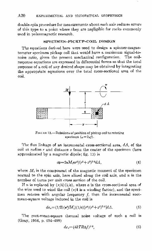
FIGURE 13. Relations of position of pickup coil to rotating specimen (« 2-n-f).
The flux linkage of an incremental cross-sectional area, dA, of the coil at radius r and distance z from the center of the specimen (here approximated by a magnetic dipole: fig. 13) is
dct>=2irMinr2/(r2 -\-22') 3/2dA, (4)
where M* is the component of the magnetic moment of the specimen normal to the spin axis, here alined along the coil axis, and n is the number of turns per unit cross section of the coil.
If n is replaced by (7r/4)(l/a), where a is the cross-sectional area of the wire used to wind the coil (?r/4 is a winding factor), and the speci men rotates with angular frequency /, then the incremental root- mean-square voltage induced in the coil is
The root-mean-square thermal noise voltage of such a coil is (Gray, 1954, p. 494-499)
de t=(4kTRAf) 1/2 , (6)
REMANENT MAGNETIZATION OF IGNEOUS ROCKS A21
where k is Boltzmann's constant, T the absolute temperature, A/ the pass band over which de t is measured, and R is the total resistance of the incremental cross-sectional area, dA, of the coil. Replacing R by 2irrp(n/a) dA = (ir2rp)/(2a2), where p is the resistivity of the wire, equation 6 becomes
de t =(Tr/a)(2kTrptf) 1/2dA. (7)
Another source of noise arises from voltages induced in the coil from ambient alternating fields in the laboratory. Assuming that there are no gradients in such fields over the area bounded by the coil, the root-mean-square voltage in the incremental cross-sectional area of the coil from these fields is «
= WHtf (WdA, (8)
where Hf is the effective peak field strength of the component of the ambient alternating field at frequency/ along the coil axis.
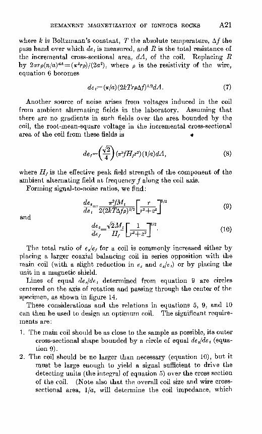
Forming signal-to-noise ratios, we find :
de t and
de, TtMt r r T'2J
T'2 '
The total ratio of e s/ef for a coil is commonly increased either by placing a larger coaxial balancing coil in series opposition with the main coil (with a slight reduction in e s and e s/e t) or by placing the unit in a magnetic shield.
Lines of equal de s/de t determined from equation 9 are circles centered on the axis of rotation and passing through the center of the specimen, as shown in figure 14.
These considerations and the relations in equations 5, 9, and 10 can then be used to design an optimum coil. The significant require ments are:
1 . The main coil should be as close to the sample as possible, its outer cross-sectional shape bounded by a circle of equal de s/de t (equa tion 9).
2. The coil should be no larger than necessary (equation 10), but it must be large enough to yield a signal sufficient to drive the detecting units (the integral of equation 5) over the cross section of the coil. (Note also that the overall coil size and wire cross- sectional area, I/a, will determine the coil impedance, which

A22 EXPERIMENTAL AND THEORETICAL GEOPHYSICS
FIGURE 14. Curves of equal incremental signal-to-noise ratio (desfde t). Dotted line shows outline of rotating equipment: A, optimum shape for the main coil; B, optimum shape of the balancing coil for the spinner magnetometer described in this paper.
should be matched to the detecting unit.) Figure 14 also shows the optimum shape of a detecting coil for the spinner mag netometer described above.
The equations also suggest high angular-rotation velocities and narrow pass bands; these factors can be considered along with others such as the desired sensitivity, ease of operation, and stability of the detecting units in the overall design of a spinner magnetometer.
COLLECTION OF SAMPLES
Although irregularly shaped samples broken from outcrops may be oriented in a variety of ways, it is often more efficient to obtain oriented samples by drilling short cores in place with portable coring equipment. The regularly shaped cores can be routinely oriented with an accuracy of 2°, and sampling need not be restricted to the edges of joint blocks.
The drilling unit we employ (fig. 15) consists of the power unit from a small commercial chain saw, a special transmission (details

REMANENT MAGNETIZATION OF IGNEOUS ROCKS A23
FIGURE 15. Sample-coring drill with water tank and orienting device.
FIGURE 16. Mechanical details of the core-drill transmission (shown about one-half size). A, Case; B, shaft; C, water inlet; D, grease fittings; E, bearings; F, seals; G, adapter to fit core drill; H, adapter to fit clutch plate; /, drill with fitting.
shown in fig. 16), a commercial sintered diamond masonry-coring drill, and pressure-type garden-insecticide spray tanks for supplying cooling water to the diamond drill. Cores 2.49 cm in diameter and from 10 to 20 cm long can be drilled from most extrusive igneous

A24 EXPERIMENTAL AND THEORETICAL GEOPHYSICS
rocks with little difficulty unless the rock is highly fractured. Hard rocks that require long drilling time may be more easily drilled by fitting the coring equipment to a tripod, or similar device, that will support the weight of the unit as well as guide the core drill. Without water in the tanks, the unit weighs about 10 kilograms.
The cores are oriented by means of slotted tubes that can be slipped over the core before it is separated from the outcrop (fig. 15). The slotted tubes are fitted with a level so that the slot may be placed along the uppermost edge of the core (intersection of the core surface with the vertical plane passing through the core axis); they are also fitted with a magnetic compass, an inclinometer, and sighting blades for transit operation. Properly fitted, a geologist's pocket transit may also fulfill all these needs.
In our system, the core axis is the z axis, positive from the surface into the outcrop, and the x and y axes define an orthogonal system, in which y always lies in the horizontal and the -\-x direction is always inclined above the horizontal; right-handed coordinates are used, so that the -\-y axis (horizontal) is directed to the right as one looks down the core axis (direction of +2).
A mark corresponding to the z axis is made along the upper edge of the core by slipping a brass or copper wire down the slot. The plunge of this line below (+) or above ( ) the horizontal is read from the inclinometer and recorded, as is the geographic azimuth of the -\-y direction, which is determined by triangulation prior to removing the core from the outcrop.
After the above operations and measurements have been repeated by normal field checking procedures, the core is removed from the outcrop and the mark along the edge is immediately made permanent by marking with a diamond scribe. At the same time, the -\-y direc tion is indicated by permanent short marks on the right side of the orientation line along the entire length of the core. In this manner each specimen later cut from the core for measurement (fig. 8) retains a complete orientation, and there is no chance of errors arising during transfer of orientation marks.
We have estimated from mechanical considerations that cores of the size described here may be routinely oriented to within ±2° using a simple slotted tube and geologist's pocket transit. If required, accuracies of ±0.5° can be achieved with cores of this size by using sufficiently precise measuring devices and by using care in placing the orientation line on the core before it is removed from the outcrop.
An additional piece of field equipment that has proved useful in collecting samples for paleomagnetic investigation is the declination gradiometer shown in figure 17 (Doell and Cox, 1962). Two small oil-damped magnetic compasses mounted in gimbals at opposite ends
REMANENT MAGNETIZATION OF IGNEOUS EOCKS A25
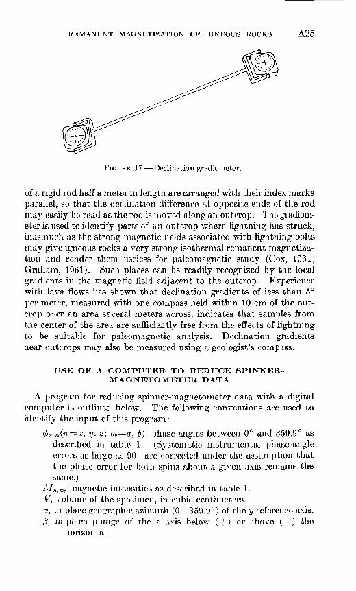
FIGURE 17. Declination gradiometer.
of a rigid rod half a meter in length are arranged with their index marks parallel, so that the declination difference at opposite ends of the rod may easily'be read as the rod is moved along an outcrop. The gradiom eter is used to identify parts of an outcrop where lightning has struck, inasmuch as the strong magnetic fields associated with lightning bolts may give igneous rocks a very strong isothermal remanent magnetiza tion and render them useless for paleomagnetic study (Cox, 1961; Graham, 1961). Such places can be readily recognized by the local gradients in the magnetic field adjacent to the outcrop. Experience with lava flows has shown that declination gradients of less than 5° per meter, measured with one compass held within 10 cm of the out crop over an area several meters across, indicates that samples from the center of the area are sufficiently free from the effects of lightning to be suitable for paleomagnetic analysis. Declination gradients near outcrops may also be measured using a geologist's compass.
USE OF A COMPUTER TO REDUCE SPINNER- MAGNETOMETER DATA
A program for reducing spinner-magnetometer data with a digital computer is outlined below. The following conventions are used to identify the input of this program:
4> n,m(n = x, y, z; m=a, b), phase angles between 0° and 359.9° as described in table 1. (Systematic instrumental phase-angle errors as large as 90° are corrected under the assumption that the phase error for both spins about a given axis remains the same.)
Mn, m, magnetic intensities as described in table 1.V, volume of the specimen, in cubic centimeters.a, in-place geographic azimuth (0°-359.9°) of the y reference axis.(3, in-place plunge of the z axis below (+) or above ( ) the
horizontal.

A26 EXPERIMENTAL AND THEORETICAL GEOPHYSICS
7, quadrant of the horizontal projection of the z axis, according to the following convention:
Azimuth y
z vertical._____________________________________ 00.1°- 89.9°_--___--____-----_-___---___-____- 1
90.0°-179.9 0 -____ ______- ---____-_--____-_--- 2180.0°-269.9° _-_______----____-_--__-__--_-- 3270.0°-359.9° ____-_--_-___-___---_-___------ 4
The following conventions are used to identify the output of this program:
D, declination, that is, azimuth of the horizontal component of of the remanent-magnetization vector restored to its in-place orientation.
/, inclination, that is, in-place plunge of the magnetic vectorbelow the horizontal.
M, total magnetic moment of the specimen. J, M/V, the magnetic intensity, in electromagnetic units per
cubic centimeter.A, an analogue of the radius of the error triangle formed by the
three great circles defined by the phase angles, as discussed below.
MM, the root mean square of the differences between the six measured magnetic intensities, Mi>a , MZi1> , and so forth, and the ideal intensities that would be expected if the specimen acted as an ideal dipole with moment M and direction of magnetization as calculated.
To find the mean direction from the three phase-angle great circles, a comparison is first made to determine whether the three circles intersect within 0.1°. If not, an increment is added to each phase angle inversely proportional to the A"th power of the corresponding intensity Mg , Mx, or Mv, where N is retained as a parameter to be specified in the program. This process is reiterated until the common intersection is found to within 0.1°. To obtain higher precision, only the single constant in step 21 (see below) needs to be changed. As a measure of the lack of closure of the original error triangle, the average total increment added to the phase angles corresponding to the two strongest intensities is recorded as the quantity A.
The best value for the parameter N depends on the relation of the accuracy of phase-angle measurements to the magnetic intensities. This relation, in turn, depends largely on physical considerations. If N is set equal to 0, all phase angles are weighted equally and the computer solution is the center of a circle inscribed in the error tri angle. This solution is undesirable because it gives too much weight to phase angles associated with very weak intensities, which tend to
REMANENT MAGNETIZATION OF IGNEOUS ROCKS A27
be less reliable. On the other hand, assignment of a large number, say 5 or more, eliminates from the calculation the phase angle associ ated with the smallest intensity, and this weighting is undesirable where the three phase angles all have approximately the same relia bility. However, for very weakly magnetized specimens where only two of the three pairs of measurements are above the background- noise level, a large A^may be required to permit rejection of the mean ingless weak measurement. On the basis of computer experiments with a wide variety of data, we have adopted a value of N=2; although no single value is adequate for all types of data, this value has proven satisfactory for almost all routine measurements made over a 2-year period.
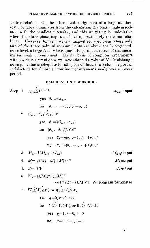
CALCULATION PROCEDURE
Step 1. 4> re , ra <180.0° 0W , M : input
yes 0re> m=4>n . m
no 0»lBI=-(360.00-<fc,, M)
2. (0,, a+0re , 6)<90.0°
yes 0re =i(0«, a 0«,»)
no (0ra , a-0re, 6)>0.0°
yes 0»=|(0 B,«-0». 6)-180.00
no -^=K«».a-^, 6) + 180.00
3. Mn =?(Mn,a+Mni t) M,,,*: input
4. M=[|(M|+M,2 +Mf)] 1/2 M: output
5. J=M/V J: output
N: program parameter
7. WZ >WX >WV or Wz >Wy>W
yes g=0, r=0, s=l
no Wx>Wg >Wy or Wx >Wy>W
yes q=l, r=Q, s=0
no <jr=0, r=l, s=0
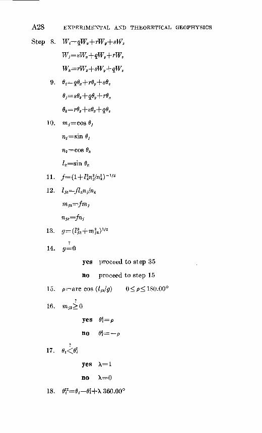
A28 EXPERIMENTAL AND THEORETICAL GEOPHYSICS
Step 8. W^
10. m^=cos
11. /=
12. l=
13. 0=
14. r=
yes proceed to step 35
no proceed to step 15
15. p=arc cos (ljk/g~) 0<p< 180.00
16.
yes 6\=p
no ^= p
17. 0<<05
yes X=l
no X=0
18. fl?=^ flJ+X 360.00°

REMANENT MAGNETIZATION OF IGNEOUS ROCKS A29
Step 19. 0IiI <180..00°
yes M=
no ju=
20. 0Ii?
21. 00P<0.07°
yes proceed to step 35
no proceed to step 22
22. 0r=0?(l TO+Kl+MW 360.00
23. 07
? 24. 0?> 180.00°
yes 0yr =:0y-360.000
no25. 4=0
yes dj= (nk cos 0T 1)/! % cos 0P|
no dj=nklk l\nkl k
26.
yes c^fc
no d
sin 0J1)/ ^ sin QVI
27.
28.
29.
n3 rrij
< -180.00°
yes ^ I?
no ^>180.00°
yes 0?=0} 360.00
no 0.I =0

A30 EXPERIMENTAL AND THEORETICAL GEOPHYSICS
?Step 30. e\< 180.00°
yes 6^= 0^+360.00°
no e\> 180.00°
yes ^=^-360.00°
no P*=6l
31. A^
32. Transfer A t to storage and accumulate for all cycles through reiterative part of program.
33. Transfer to step 10 and replace
*« by 6^
h by 8%
34. Reiterate steps 10 through 33 until yes option in step 21 is reached, or until 10 reiterations have been completed. In latter procedure, stop calculation and print "NO." Omit steps 25 and 26 on each reiteration, retaining the values of dj and dk from the first cycle.
35. l=sljk +rmjk+qnjk
n=rljk+qmjk+snjl:T
A: output36. A=
where T is the total number of reiterations through steps 10-33.
37. M'z=M[l2+m2 ] 1/2
M'x =M[m2 +n2 ] 1/2
My =M[n2+l2 ] lf2
38. MM= (1/2.449M)[ (M'f-Mt. a) 2 + (M'f -Mg , 6) 2 + (M'X -MX< a) 2
MM: output

REMANENT MAGNETIZATION OF IGNEOUS ROCKS A31
Step 39. 7=0?
yes 0=90.0°
yes x= 180.0° skip steps 40, 41
no x= 0.0° skip steps 40, 41
no «<90.0°
yes 5=1
no a<180.00°
yes 5=2
no a<270.0° yes 5=3 no 5=4
40. (5-7) = ! or (5-7) = 3
yes e=0
no (5 7) = ! or (5 7) =3
yes e=l
no stop calculation, print out "QE"
41. X=90.0°-/3+e(2/3+180.0°)
42. l' = l cos X+TI sin X
n' = l sin x-\-n cos X
43. 7=arc sin n', 90.0°</<90.0° /: output
44. X=m cos a-\-l' sin a
F=m sin a-\-l' cos a
45. D'=arc cos [X/(X2 -\-Y2^]Q.O°<D f < 180.0°
46. Tr >0.0°
yes D=D' D: output
no #=360.0°-£>'

A32 EXPERIMENTAL AND THEORETICAL GEOPHYSICS
REFERENCES
Bruckshaw, J. M., and Robertson, E. I., 1948, The measurement of magneticproperties of rocks: Jour. Sci. Instruments, v. 25, p. 444-446.
Cox, Allan, 1961, Anomalous remanent magnetization of basalt: U.S. Geol.Survey Bull. 1083-E, p. 131-160.
Doell, R. R., and Cox, Allan, 1962, Determination of the magnetic polarity of rocksamples in the field: U.S. Geol. Survey Prof. Paper 450-D, Art. 151,p. D105-D108.
1963, The accuracy of the paleomagnetic method as evaluated fromhistoric Hawaiian lava flows: Jour. Geophys. Research, v. 68, No. 7,p. 1997-2009.
Graham, J. W., 1949, The stability and significance of magnetism in sedimentaryrocks: Jour. Geophys. Research, v. 54, no. 2, p. 131-167.
Graham, K. W. T., 1961, The re-magnetization of a surface outcrop by lightningcurrents: Geophysics Jour., v. 6, no. 1, p. 85-102.
Gray, T. S., ed., 1954, Applied electronics: 2d ed., New York, John Wiley & Sons,881 p.
Johnson, E. A., and McNish, A. G., 1938, An alternating-current apparatusfor measuring small magnetic moments: Terrestrial Magnetism and Atmos pheric Electricity, v. 43, p. 393-399.
Nagata, Takesi, 1961, Rock magnetism: revised ed., Tokyo, Maruzen Co.,Ltd., 350 p.
U.S. GOVERNMENT PRINTING OFFICE: 1964 O 745-239