Embed Size (px)
Citation preview
Measurement of the Top Quark Pair Production Cross Section
and Simultaneous Extraction of the W Heavy Flavor Fraction
at√
s = 7 TeV with the ATLAS Detector at the LHC
Dissertation
zur Erlangung des mathematisch-naturwissenschaftlichen Doktorgrades
”Doctor rerum naturalium”
der Georg-August-Universitat Gottingen
vorgelegt von
Adam Roe
aus New York City, NY, USA
Gottingen, 2012

Referent: Prof. Dr. Arnulf QuadtKorreferent: PD Dr. Jorn Große-Knetter
Tag der mundlichen Prufung: 22. Marz 2012

Measurement of the Top Quark Pair Production Cross Sectionand Simultaneous Extraction of the W Heavy Flavor Fraction
at√
s = 7 TeV with the ATLAS Detector at the LHC
von
Adam Roe
The top quark pair production cross section, σtt, is measured in the semilep-tonic channel in two datasets using a binned profiled likelihood template fit todata to discriminate the signal, tt, from its main background, the productionof a W -boson in association with jets (W+jets). Templates in the first analy-sis are derived from a four variable flavor-sensitive discriminant to measure σtt in∫
L dt= 35 pb−1. A similar but flavor-insensitive discriminant is then used to mea-sure σtt in
∫
L dt = 0.7 fb−1. A third analysis is presented which simultaneously fitsthe fractions of tt and W+jets events in which heavy flavor jets are produced, usinga single flavor-sensitive distribution in the
∫
L dt = 0.7 fb−1 dataset. Experimentalprecision of the top quark pair production cross section surpasses the theoreticaluncertainty. No significant deviations from predictions are found but the results arehigher than expectation.
Post address:Friedrich-Hund-Platz 137077 GottingenGermany
II.Physik-UniGo-Diss-2012/04II. Physikalisches Institut
Georg-August-Universitat GottingenApril 2012


It would be so nice if something made sense for a change!
– Alice in Wonderland, Lewis Carroll


Contents
1 Introduction 31.1 The Scientific Process . . . . . . . . . . . . . . . . . . . . . . . . . . . . . . . . . 6
2 Theoretical Background 92.1 The Standard Model of Particle Physics . . . . . . . . . . . . . . . . . . . . . . . 92.2 The Top Quark . . . . . . . . . . . . . . . . . . . . . . . . . . . . . . . . . . . . . 142.3 Cross Section Predictions at Hadron Colliders . . . . . . . . . . . . . . . . . . . . 16
3 Experimental Environment 25
3.1 The LHC Accelerator . . . . . . . . . . . . . . . . . . . . . . . . . . . . . . . . . 253.2 The ATLAS Experiment . . . . . . . . . . . . . . . . . . . . . . . . . . . . . . . . 29
4 Reconstruction and Definition of Physical Objects 354.1 Event Level: Data Streams, Triggers, and Event Cleaning . . . . . . . . . . . . . 354.2 Object Reconstruction and Selection: Jets, Muons, Electrons, and Missing Energy 39
4.3 Selection Summary . . . . . . . . . . . . . . . . . . . . . . . . . . . . . . . . . . . 484.4 The b-tagging Algorithms . . . . . . . . . . . . . . . . . . . . . . . . . . . . . . . 48
5 Modeling of Signal and Background Processes 535.1 Monte Carlo Simulation of Physical Processes . . . . . . . . . . . . . . . . . . . . 535.2 Estimating “Fake” Lepton Kinematics and Rate . . . . . . . . . . . . . . . . . . 57
6 The Profile Likelihood Fit 63
6.1 The Profile Likelihood . . . . . . . . . . . . . . . . . . . . . . . . . . . . . . . . . 636.2 Evaluation of Uncertainties . . . . . . . . . . . . . . . . . . . . . . . . . . . . . . 66
7 Measurement of σtt in∫
L dt= 35 pb−1 Using b-tagging 717.1 Selection . . . . . . . . . . . . . . . . . . . . . . . . . . . . . . . . . . . . . . . . . 717.2 The Input Distribution . . . . . . . . . . . . . . . . . . . . . . . . . . . . . . . . . 71
7.3 The Fit Likelihood . . . . . . . . . . . . . . . . . . . . . . . . . . . . . . . . . . . 747.4 Results of the Fit and Systematic Uncertainties . . . . . . . . . . . . . . . . . . . 77
8 Measurement of σtt in∫
L dt = 0.7 fb−1 Without b-tagging 898.1 Selection . . . . . . . . . . . . . . . . . . . . . . . . . . . . . . . . . . . . . . . . . 898.2 The Input Distribution . . . . . . . . . . . . . . . . . . . . . . . . . . . . . . . . . 898.3 The Fit Likelihood . . . . . . . . . . . . . . . . . . . . . . . . . . . . . . . . . . . 91
8.4 Results of the Fit and Systematic Uncertainties . . . . . . . . . . . . . . . . . . . 91
9 Simultaneous Measurement of σtt, fWHF, and fWc in
∫
L dt = 0.7 fb−1 1059.1 The Input Distribution . . . . . . . . . . . . . . . . . . . . . . . . . . . . . . . . . 1069.2 The Fit Likelihood . . . . . . . . . . . . . . . . . . . . . . . . . . . . . . . . . . . 1079.3 Results of the Fit and Systematic Uncertainties . . . . . . . . . . . . . . . . . . . 110
iv

Contents
10 Interpretations of Results and a Glance Towards the Future 12110.1 The Meaning of These Results . . . . . . . . . . . . . . . . . . . . . . . . . . . . 12210.2 An Outlook: The Coming Precision . . . . . . . . . . . . . . . . . . . . . . . . . 124
A Summary of Systematic Uncertainties 127
B Kinematic Comparison of tt in MC@NLO and POWHEG 129
C Control Plots for the∫
L dt= 35 pb−1 Dataset 133
D Control Plots for the∫
L dt = 0.7 fb−1 Dataset 141
Bibliography 157
Acknowledgements 167
v


1 Introduction
The title of this thesis proposes to measure the top quark pair production cross section at theLarge Hadron Collider using the ATLAS experiment, that is, to determine experimentally therate of one of the many possible outcomes in a high-energy proton-proton collision. The precisemeaning of this task and understanding of possible results warrants discussion.
Much interpretation is done. What is truly measured is the energy deposited by, or momentumof, particles which in fact are the decay remnants of the particles of interest. In some cases, theparticles which are measured are several steps away along a decay chain. Using our knowledgeof interactions of particles with matter built over the past hundred years, we can associate theseprimal measurements – a charged particle’s trajectory through a tracker, a deposit of energy ina calorimeter – with specific particles, making the first leap necessary. Such traces left acrossthe detector allow for the reconstruction of a single physical object: an electron, muon, or a jet(coming from a quark, for instance).
The neutrino has posed experimentally and philosophically challenging questions since itsproposal in 1930, and in the present collider environment, their detection not feasible [1]. Incertain recent experiments designed specifically for neutrino detection, it has proved only tobe a technical challenge: the small probability of a neutrino interacting with matter has leadto the use of extraordinary masses in experiments, so large in fact that experiments are evenusing Antarctica or the Mediterranean Sea as a part of their detector. In such experiments, theneutrino is no more abstract than the nucleus was in the gold foil experiment [2, 3]. This is notthe case here, where the neutrino here is signified by an absence of direct signal in the detector.
Let us presume that the necessary departure from positivism caused by the high poweredabstractions of our scope are not problematic. The association of the particles with a parentfrom which they have decayed is, to some extent, the issue at hand in this thesis. The particlesobserved in a single collision event are collectively known as the final state. The signal understudy is pairs of top quarks produced in collision. Both top quarks decay into a W boson and ab-quark, where one W subsequently decays into a charged lepton and a neutrino while the otherdecays into two quarks. Each of the four quarks present forms a jet, which can be observed. Atypical final state in the measurements presented here is therefore four jets, a charged lepton(electron or muon) and large missing energy (a neutrino). Events here are identified using thelepton, naturally dividing the semileptonic channel further according to lepton flavor, e+jetsand µ+jets. Those are further subdivided by the number of jets in the event, since it may havemore or less than four.
There are several other mechanisms known in the Standard Model which can create this finalstate. In this thesis, the results are obtained assuming that those and only those processescontribute to the data sample. Beyond the production of tt, the main process which can createthe same final state is the direct production of a W boson in association with jets. Smaller con-tributions are expected from other electroweak processes.The signal as well as these backgroundprocesses are modeled using Monte Carlo (MC) simulation [4]. The tools which implement basictheoretical predictions as MC are known as generators.
The production of a multijet final state in which one of the objects is misidentified as anisolated, prompt lepton also creates the same experimental final state. This process is difficult to
3

1 Introduction
model as it is fundamentally an effect of experimental limitation, arising from a false assignmentof the measured energy and momentum. The rate of the underlying physical process in a givenenergy range is naturally very high, so much so that even a small rate of lepton misidentificationcan cause a significant contribution from this process to the selected data sample.
On an event-by-event basis, it is impossible to distinguish the various physical processes fromone another. In other words, if a single event with such final state is observed, one cannot saydefinitely which of those physical process occured in the proton-proton collision. There are manyways to use the observed events in a measurement, but two will be focused on in particular inthis discussion. One can take for granted the presence of the background processes and attemptto establish an excess of events in the form of a signal, as has been done in the first paper fromATLAS measuring top pair production cross section, σtt [5]. The theoretical assumptions wouldthen be that the full number of events is described by the SM and that σtt is the only unknown,that branching ratios for the decays of the processes involved including top quarks are known,and that differential predictions in the form of MC can model the percentage of the processwhich will be observed (acceptance and efficiency). Such a cut-and-count method was used toestablish the signal in that first paper. This is not precisely the route followed in this thesis.
In the analyses presented, differential theoretical predictions are used to discriminate themechanisms which produce the final state under study, effectively allowing one to claim, fora given event, that it is more likely to arise from a certain physical process or another, butcertainly not allowing a definitive statement of origin on an event-by-event basis.
Taking a relatively traditional approach, one may ask what hypothesis we are testing. Thenaive answer may be “The Standard Model”. The first papers published using the cut-and-count method with early data already showed that the observed cross section is in the samerange as predictions, albeit with a large experimental uncertainty [5, 6]. Yet it is extremelydifficult to make a precise prediction for a production cross section in proton-proton collisionsfor the process of interest here. This difficulty is due mostly to the complications of the theoryof the strong force, Quantum Chromodynamics (QCD), and partially to our lack of knowledgeof the proton. Predictions are done with QCD using perturbation theory, approximating it bya series expansion around the strength of the force. One must always choose to which order itwill be expanded, where higher-order corrections are typically of less importance and harder tocalculate. A more precise measurement, such as those presented here, does not therefore test theStandard Model in general but rather tests specific predictions made with it at a given precision.
Different signal models exist, one of which has to be assumed, even though none of them isa priori more correct than another. The degree of theoretical knowledge becomes a relativelylarge uncertainty at the level of precision currently available.
The best differential predictions available and implemented in MC simulation are at secondorder, Next to Leading Order (NLO), while non-differential “inclusive” cross section predictionsare approaching one order more of precision, known as approximate NNLO. For the productionof tt we use NLO kinematics for the core process with approximate NNLO normalization1. Mostof the background processes are only available at one order lower, that is, LO kinematics withNLO normalization. The hypothesis may then be that “QCD NLO kinematics and NNLO ratepredict the behavior of top quark pairs produced in proton-proton collisions at the LHC”.
This hypothesis itself raises several questions. Are NLO kinematics for the process well pre-dicted? Is approximate NNLO well defined? Does it make sense to combine NLO kinematicswith NNLO inclusive predictions? What would be the implications if the result of the analysisis not compatible with the hypothesis?
1Throughout this thesis, the kinematics present in NLO MC generators will be referred to simply as “NLO” andthe inclusive approximate NNLO predictions as “NNLO”
4

There are two main NLO MC generators available for the prediction of tt which will beused in this thesis. They are hitherto equally valid2. Considering the reliance on this to makepredictions, be it for calculating signal acceptance or for more complete kinematics as in theseanalyses, one could use one and not the other and test the hypothesis using a single generator.The hypothesis then becomes “QCD NLO kinematics as predicted by Generator X and NNLOrate predict the behavior”. It could of course be tested for the other as well. What is donehere instead is that one generator is taken to be the baseline and the other is used to evaluatepotential bias as a systematic uncertainty. Doing so thereby retains the more general hypothesisof testing NLO kinematics, taking the two generators as representative of the difference. Oneof three analyses presented in this thesis includes the possibility to learn if one or the other isfavored as a model of the data.
A study has been undertaken to examine the uncertainty on acceptance of the signal processat NLO. The ratio of the fiducial cross section to the fully inclusive cross section is defined3.The fiducial cross-section is calculated using truth-level kinematic cuts corresponding to thosein the analysis. The theoretical prediction for both the inclusive and fiducial cross sections arevaried within their uncertainty, by the standard method of changing the renormalization andfactorization scales by a factor of 2, and the change in the ratio is observed. We have learnedthat the effect of the scale variation on this ratio is in fact rather dependent on the number ofjets considered in the analysis. Requiring at least four jets, as is often done in such analyses,yields a difference in the ratio of as much as 10 %. Only by requiring at least three jets arethe migration effects mitigated, and the change in the ratio becomes ≈ 2 %. In the analysespresented here, at least two or three jets are required, so the ratio is well defined. This simplestudy indicates that using NLO predictions for precisely measuring σtt cannot be done withoutthe inclusion of events with a 3-jet final state in addition to those with higher jet multiplicities.
There are various approximate NNLO predictions for σtt. Any measurement in the range ofabout 140-180 pb would be found to be consistent4. In other words, one can consider approximateNNLO predictions for mtop = 172.5 GeV to be about 158± 18 pb, about a 12 % uncertainty. Ofthe various approximate NNLO predictions available, a single value is used for comparisonthroughout this thesis, but it is important to know that there are other estimations available.The NLO MC simulation is normalized to the NNLO cross section using a non-differential “k-factor”, in essence assuming that the ratio σ(NLO)/σ(NNLO) is not phase-space dependent.This is not necessarily a physically sound assumption, however doing so allows for comparisonwith the most precise theoretical results available. Normalizing the MC simulation to theoreticalpredictions using non-differential k-factors will be done throughout this thesis.
The results presented here find final uncertainties on the top pair production cross section inthe range of 6-13 %. The experimental uncertainty is therefore smaller than the theoretical, andin fact by now a huge portion of the experimental uncertainty is due to theoretical dependence.What then, would be the implications, if the measurement does not agree with the theoreticalpredictions? First and foremost, it would in fact be difficult for them not to agree given theinterdependence of theory and experiment. If they are not in perfect agreement either – which
2An excellent, hot-off-the press review of methods and differences is available in [7]. The two generators usedhere are MC@NLO[8, 9] and POWHEG[10]. A very interesting comparison of them can be found in [11],which highlights the differences between the two and related issues.
3MCFM [12] is used for the numerator while the denominator uses Hathor [13] evaluated at NLO. Details ofthis study are given in Appendix C of [14].
4The prediction used by the ATLAS collaboration and throughout this thesis is σtt=164+11−16 pb [13]. Other
predictions such as σtt=154+15−14 pb exist as well[15]. It should be noted that the latter value uses a slightly
higher value for mtop, suppressing the cross section. About half of the discrepancy between the predictionsseems to be numerical choices including the mass difference and the other half methodological.
5
1 Introduction
they also cannot be, except by chance – predictions which do not agree may be tweaked, at whichpoint they cease to be predictions and become descriptions. If the measurements are a bit wideroff the theoretical mark, it could easily be claimed that higher order predictions are needed.This is the essence of the hypothesis: if a discrepancy is found, it is not with the underlyingtheory itself but rather with the best available predictions using the theory. The theory of QCDis not being tested here, but rather the precision of the estimates using it are. This is all themore so the case in the measurement of the production of W bosons with associated heavy flavorjets, whose theoretical uncertainty is on the order of 50-100 %, meaning a measurement wouldhave to be nearly an order of magnitude different from predictions to bring into question ourunderstanding of the underlying physical processes. In this case, it is rather that theoreticalpredictions need experimental input than that precision predictions are being tested.
1.1 The Scientific Process
Never before has scientific collaboration on the scale of the LHC and its experiments beenundertaken: the two main experiments each have nearly three thousand active scientists whoare taken to be the authors of the papers published by the respective collaboration. The size ofthe collaborations implies a necessary departure from certain tenets of traditional science. Thescientific work is considered to be truly collaborative, as evidenced by the fact that papers arepublished by the collaboration and not individuals. A great deal of input from the collaborationis used in any physics analysis. More than 100 papers have been published by the ATLAScollaboration at time of writing, all of which have an author list of about 3,000 physicists listedalphabetically. To qualify as an author one must meet basic criteria intended to show continueddedication to the collaboration, such as periodically taking part in the acquisition of data ormonitoring of the detector. The author of this thesis has contributed in particular to the real-time monitoring of the pixel subsystem of the experiment, both in developing software used inmonitoring and doing so.
The data are recorded centrally, with a handful of physicists sitting in the control room at agiven time in charge of the process. Algorithms to process the raw data are also run centrally, andthe data are made available to the entire collaboration. Physicists self-organize into groups, someof which are responsible for a part of the detector or given final state observable particle, whileothers are organized by topic of underlying physical interest. These group calibrate the detector,maintain reconstruction algorithms, estimate uncertainties, and make general recommendations.
The work described in this thesis relies on the ATLAS collaboration. The details of objectdefinition and uncertainty described in Chapter 4 are common to those studying the top quarkand to some extent the entire collaboration. The author has contributed to a handful of topics,in particular to the definition of the electron and in optimizing kinematic cuts in the e+jetschannel in the context of reducing the fake contribution.
An additional effect of the size of the collaborations is that any analysis undergoes an extensiveinternal review by the collaboration prior to submission to a journal. In ATLAS, the processof publishing a paper goes through many steps, first receiving approval from the related groupbefore being sent for collaboration-wide review. This is followed by a final sign-off from thecollaboration leadership before being submitted to a journal. It is generally assumed that anypaper submitted by one of the large collaborations will be published. A streamlined versionof this process exists for “preliminary” results, in particular for international conferences. Thestandards required to be met for the paper publication procedure are generally higher than thosefor a preliminary result.
6

1.1 The Scientific Process
The measurement of the top pair production cross section using the 2010 data which is pre-sented in Chapter 7 of this thesis was first shown by the collaboration at the Moriond QCD andHigh Energy Interactions conference [16]. After ten months of review, this work was submittedby the collaboration as a paper to Physics Letters B [17]. In the meantime, a similar analysisusing a significantly larger dataset recorded in the first half of 2011 was performed and presentedby the collaboration at the Lepton Photon conference [18], presented in Chapter 8. The finalanalysis in this thesis presented in Chapter 9 has not been subjected to the approval procedureand is therefore not in any way an official result from ATLAS.
In addition to the structure of the collaboration described, the analysis team is often comprisedof a few people working very closely together. In the case of the analysis methodology presentedin Chapter 6, the concept was developed by a team of a few students, including the author,and postdocs, working together. The publicly presented analyses themselves are the productof direct work from this small group of researchers. It is somehow natural for no more than afew people to work together intensely, constantly. On this scale agreement can be reached thatsatisfies the concerns of those involved without formal procedure. This is where, absent theshackles of politics, scientific rigor is truly achieved.
7

Depth. “The Planck length is another thousand or two pixels below the comic.”[19]

2 Theoretical Background
An overview of current knowledge of fundamental particles and their interactions will be givenhere. The special case of the top quark, the object under study in this thesis, will be discussed.The theoretical predictions for top quark pair production cross section in collisions at the LHCwill be reviewed, along with predictions for W+jets production, in particular with heavy quarkjets in the final state.
2.1 The Standard Model of Particle Physics
The Standard Model of Particle Physics (SM) contains our state-of-the-art knowledge of ex-perimentally fundamental particles and their interactions. Six quarks and six leptons (all spin1/2 fermions) are the building blocks of matter while four known force carriers (spin 1 bosons)are the quanta of their interactions. Our knowledge of the properties and interactions of theseparticles has been built over the last hundred years through experiment and interpreted in theframework of quantum field theory (QFT), the relativistic field theory of quantum mechanics.The Standard Model as it is currently conceived of will be reviewed here.
The quarks and leptons are understood as three generations each of 2 quarks and 2 leptons.The traditional arrangement of these three generations follows the historical development oftheir discovery which, for reasons of energy requirements, follows the increasing rest mass of theparticle (except for possibly in the case of neutrinos). Each generation is composed of an “up-type” quark with electric charge Q=+2/3 and a “down-type” quark with Q= -1/3, as well as acharged lepton with Q=-1 and an electrically uncharged neutrino. All particles have antimatterpartners with opposite quantum numbers but identical mass.
In our current understanding, these particles are fundamental: there is no evidence that anyof them can be broken into constituents and they are treated with the same mechanisms inQFT. The properties of these particles are not identical, giving rise to their varied behavior.
In moving from one generation to the next, the two things which change are the mass of theparticle and its “flavor” which is described by its name. The three generations can be arrangedas
(
u (up)d (down)
) (
c (charm)s (strange)
) (
t (top)b (bottom)
)
(
νe (e neutrino)e (electron)
)(
νµ (µ neutrino)µ (muon)
)(
ντ (τ neutrino)τ (tau)
)
The fermion masses are free parameters in the SM and are of great interest. They are measuredexperimentally and input to the theory. Using the lagrangian formalism, the Dirac equationdescribing a free spin-1/2 particle of mass m with wave function ψ can be written as [20]:
Lfree = ψ(i/∂ −mf )ψ
The mass of a particle affects its behavior strongly. In part this is due to considerations ofenergy: a heavier particle will decay into lighter particles if it is possible. The lightest particles
9

2 Theoretical Background
are thus stable; the material found in the Periodic Table of Elements can be understood as beingbuilt of the first generation of particles. The mass also affects particles in more subtle ways, dueto the extraordinarily large range of masses present: the neutrinos have masses below 2 eV1 [21]while the top quark has a mass of hundreds of GeV [22], thereby spanning at least elevenorders of magnitude. An example of the difference in particle behavior caused by the magnitudeof the particle masses is the relatively recent discovery of neutrino oscillations amongst flavorstates [23]. This implies that neutrinos do indeed have mass, but so far only mass differenceshave been measured and upper limits on the mass have been set [24, 25, 26, 27]. The phenomenonof neutrino oscillation is not itself a physical interaction but exists naturally in the theory ofparticles. One may ask therefore if other particles oscillate as well. Recent work has shownthat other particles – the charged leptons, for instance – could in principle oscillate as well, butthat the mass difference between the generations is so much larger than for the neutrinos thatobservation is not particularly feasible [28]. It is the small mass difference (squared) amongstthe generations which causes observable oscillations in the neutrino system.
The Interactions of Particles in the Standard Model
There are four known fundamental forces of nature – electromagnetic, weak, strong, and grav-itational – each governing the interactions of particles based on their properties, the electriccharge, weak isospin, color charge, and mass, respectively. All except for gravity are understoodin the context of QFT and are a part of the SM. The electromagnetic and weak interactionsare known to be different low-energy manifestations of the same force, the electroweak force.The SM therefore describes two fundamentally different forces, electroweak and strong, usingQFT. The quantum field theory of electromagnetism will be considered first, then electroweakunification and the symmetry breaking into weak and electromagnetic forces, and finally thetheory of the strong force will be discussed.
Renormalization
An essential concept in QFT is renormalization, a consequence of which is that fundamentalparameters become a function of energy. Renormalization dictates the dependence of a pa-rameter on energy. An example which will be further discussed is that the coupling of a forceis α = α(Q2), where Q2 is an energy scale relevant to the process (such as energy transfer).Sometimes the bare coupling will be written as g, which is related to α by g = 4πα.
Electromagnetism and Quantum Electrodynamics
The strength of the electromagnetic interaction is proportional to the electric charge, q. Itsexchange boson, the excitation of its quantum field, is the photon, γ. The photon is a massless,spin-1 particle. The coupling of the field is the electric charge,
αEM = q2e ≈ 1
137.
The charge of the electron is therefore a fundamental parameter in the SM. Quantum Electro-dynamics (QED) predicts very precisely the dependence of many observables on αEM.
1In natural units, ~ = c = 1, will be used throughout. In these units, energy, momentum, and mass are allexpressed in units of energy.
10

2.1 The Standard Model of Particle Physics
The electromagnetic interaction is symmetric under global U(1)q transformations, correspond-ing to conservation of electric charge. The electromagnetic field is quantized, and the lagrangianfor a particle of charge Q can then be written as
LEM = −1
4FµνFµν − iαEMQψγ
5Aµψ
in the Lorentz gauge, where Aµ is the electromagnetic vector potential and Fµν is the elec-tromagnetic field strength tensor, defined as Fµν ≡ ∂µAν − ∂νAµ. Together with the Diracterms for the interacting particles in question (as shown in 2.1), the lagrangian for QuantumElectrodynamics is specified.
The Weak Force and Electroweak Theory
The weak interaction was first proposed as a four-point interaction by Fermi to explain nucleardecay. A dimensionful coupling constant was proposed to describe the interaction, now measuredto be GF ∼ 10−5 GeV−2 [29]. This was an effective theory; the units are incorrect for it to be afundamental constant. Understanding of the interaction after the discovery of parity violationlead to the inclusion of “handedness” into the weak theory [30], and eventually the unificationof the electromagnetic and weak forces into the electroweak force.
The left handed state or a right handed state of a particle is defined by the chiral projectionoperators, such that ψleft = 1
2 (1−γ5)ψ = Lψ and ψright = 12(1+γ5)ψ = Rψ. Each of the doublets
of quarks or leptons is a left-handed weak isopsin doublet, while the right-handed particles aresinglets. The symmetry of the weak interaction is SU(2)L where L stands for “left”. A three-component field Wµ is introduced which corresponds to this symmetry. The weak field strengthtensor has a form similar to the electromagnetic field strength tensor, except that the generatorsof SU(2) yield a non-Abelian term, physically representing self-coupling amongst the gaugebosons. The tensor is then defined as
F aµν ≡ ∂µW a
ν − ∂νW aµ − gW fabcW b
µWcν .
The symbol fabc is the generator of the symmetry group; physically it implies self-couplingamongst the exchange bosons with the coupling gW . For the SU(2) group, fabc is the fully-antisymmetric tensor εabc. The symmetry of SU(2)L cannot, however, be exact: it would implythree massless gauge bosons mediating the force, which do no exist. The conundrum is solvedby proposing the unification of electromagnetism and the weak force, known as electroweakunification [31, 32, 33]. This proposed symmetry still has the awkward issue that it must bebroken. Before symmetry breaking, the field lagrangian can be written as:
Lelectroweakfield = −1
4F a
µνFµνa − 1
4FµνFµν .
Here the three-index tensor represents the “pure” weak fields Wµ while the two-index tensorhas the same form as the electromagnetic field. In order to incorporate electromagnetism,hypercharge Y is defined, which is a combination of both the electric charge and the weakisospin component (I), defined as Y = 2(Q − I). The charge symmetry of electromagnetismbecomes hypercharge. The unification of the electromagnetic and weak forces into a single theorymeans that electroweak symmetry can be understood to be SU(2)L⊗U(1)Y .
The breaking of this symmetry is proposed to give mass to the quanta of the field Wµ, and inthe process must therefore preserve only the simple electric charge symmetry and the masslessphoton field, a process which can be understood as SU(2)L⊗U(1)Y → U(1)q [34]. Through
11
2 Theoretical Background
the process of electroweak symmetry breaking, the fields mix by simple rotation which can beparameterized as an angle, known as the weak mixing angle, θW. The theory therefore predictsthree massive bosons and one massless: two neutral, the familiar massless γ as well as themassive Z0, and two charged, W±. The mixing of these fields relates the masses of the heavybosons by θW and to GF to identify a dimensionless coupling by
M2W =
g2
4√
2GF sin2 θW, M2
Z = M2W/ cos2 θW.
The weak force is therefore not weak compared to electromagnetism because of a small couplingbut rather because of the large mass of its interacting bosons.
The electroweak symmetry breaking mechanism in the SM has an additional consequencewhich is the prediction of an additional boson, the scalar Higgs boson [35, 36]. The electroweaktheory has been extremely successful in general, but the Higgs boson – whose mass is notpredicted by the theory – has eluded discovery for nearly fifty years. The collaborations at theLHC have made extraordinary progress in the search and indeed have ruled out its existenceover nearly the complete mass range, save for 115 < mH < 127 GeV [37, 38]. If the SM Higgsexists, it must be in that mass range; if it does not exist, something else must be responsible forelectroweak symmetry breaking. Electroweak theory is too successful for most physicists to doubtthe theory in general and therefore expect an electroweak symmetry breaking mechanism evenif the Higgs boson is not found. Accordingly there are few if any paradigm shifting approachesto this problem, rather, another mechanism (of which there are many) would be fit into thetheory.
The Strong Force: Quantum Chromodynamics
To a great extent the force under study in this thesis is the strong force, elucidated throughthe theory of Quantum Chromodynamics (QCD). It is the dominant force amongst protons andtheir constituents in collision at the LHC. There are three “color charges” which are conservedin the theory, making it SU(3)color symmetric. Eight gluon fields are required to describe theinteractions predicted by the generators of the group. All matter which interacts via the strongforce is known as hadronic, hence the name “Large Hadron Collider” (Large refers to the size ofthe accelerator, not the hadrons).
Particles which are color charged (e.g. quarks) interact via the massless, spin-1 gluon, g.Quarks experience a phenomenon known as color confinement: only color-neutral particles arestable. This can be accomplished by pairing two quarks together which are color-anticolor andtherefore form a 2-quark state known as a meson, such as the pion. It can also be constructedout of one quark of each color (following the analogy of stage lights) to form a three-quark stateknown as a baryon, of which the proton and neutron are examples. Searches for hadronic matterwith more than 3 quarks have been performed, and indeed evidence for such states has recentlyemerged [39]. In order to conserve color, gluons must carry color charge as well.
The field strength tensor is written with the same form as for the weak interaction, howeverthe coupling constant is that of the strong force, gs, and the generators of the SU(3) group aredifferent. As in the weak interaction, the non-Abelian term predicts the self-interaction amongstgluons, both as a 3-gluon interaction and as a 4-gluon interaction. In electroweak theory thelarge mass of the bosons mitigates effects from such self-interaction terms, while in QCD thegluon being massless leads to low energy divergences in the theory. The coupling also implies thepossibility of a bound gluon state known as “glueballs”, a bound state with no valence quarks,
12

2.1 The Standard Model of Particle Physics
which has not been observed [40]. The lagrangian for QCD is then written as [41]
LQCD =∑
quarks
ψa(i/∂ −mf )abψb −1
4F a
µνFµνa + Lgauge fixing,
where the roman indices specify color charge and F aµν is the strong force field strength tensor.
The coupling constant in QCD, αs(Q2) is renormalized as in the other theories, predicted by
the beta function of QCD, β(αs). This can be expanded around αs(Q2), currently known up to
a precision of α5s [42, 43]:
β(αs(Q2)) ≡ Q2∂αs(Q
2)
∂Q2= −β0α
2s − β1α
3s − β1α
4s − β1α
5s +O(α6
s)
The constants βi are expressed by simple formulae depending on the number of quark flavorspresent, Nf . At first order, for instance, β0 = 11 − 2/3 × Nf , implying that β0 is positive forNf < 16 and therefore that the β function as a whole is negative [44, 45]. For the six knownquark flavors, β stays negative to all known orders. The energy dependence is also found to belogarithmic; at leading order αs ∼ 1/ln(Q2/Λ2
QCD), where the “scale” of QCD, ΛQCD, has beenintroduced. At energies near or below ΛQCD, the perturbative approach breaks down. The factthat the coupling decreases logarithmically with increasing energy leads to the extraordinaryproperty known as asymptotic freedom: high-energy quark becomes free from the strong force2.The theory of QCD predicts this running, but an input value for αs is needed. The most preciselymeasured value comes from measurements at the Z-mass pole, recently combined to [48]:
αs(MZ) = 0.1184 ± 0.0007.
This can be translated into a value for the scale of the theory, ΛQCD = 213± 9 MeV. Above thisscale, as in the hard interaction of protons considered in this thesis, perturbative QCD is valid.
Standard Model Summary
The Standard Model of Particle Physics can be summed up as a lagrangian with many differ-ent components describing the fundamental particles and their interactions, which have beensketched out here. Perturbative expansion around the coupling constants of the forces can beused to make predictions for observations in a collider environment using the Feynman rules.The examples most relevant to this thesis will be discussed in Section 2.3. A wealth of pre-dictions have been made with these theories which have been tested, in some cases to greatprecision, with rare discrepancy. The Standard Model accounts for a great deal of observedphenomena and has successfully made a number of predictions. It certainly does not answerall of our questions and there are many “Beyond the Standard Model” theories to tackle them,but to date there is no accepted, coherent view of any particles or interactions aside from thosementioned here.
2This is such an impressive result that it warranted not only a Nobel Prize but also a reference on populartelevision[46, 47].
13

2 Theoretical Background
2.2 The Top Quark
Amongst the particles discovered, the top quark stands out for its exceptionally large mass.Apart from its mass (and flavor of course) it is indistinguishable from the up and charm quarks,but the mass is so much larger that its behavior is unique amongst the quarks. Theoretically, thelarge mass means that it often enters into loop calculations at different orders of magnitude thanother quarks, in particular into Higgs mass loop corrections. A particle’s coupling to the Higgsfield is proportional to its mass, thus the top quark, being the most massive known particle, hasthe strongest known coupling to it. Furthermore the mass of the top quark is of the same orderof magnitude as the scale of electroweak symmetry breaking, raising the intriguing possibilitythat the top quark plays a special role in it.
Prediction and Discovery of the Top Quark
The top quark had been widely expected to exist since the discovery of the bottom quark in1977, needed in order to complete the third generation quark doublet [49]. The third generationof quarks was in fact predicted by the work of Kobayashi and Maskawa amongst others, whoextended the then 2× 2 Cabibbo matrix into the now familiar 3× 3 CKM matrix in order toaccount for CP-Violation in the weak interaction, work for which the Nobel Prize in Physicswas recently awarded [50, 51]. Searches for the top quark, at CERN’s Large Electron PositronCollider (LEP) in particular, placed lower limits on the mass of the top quark before it wasdiscovered [52]. To do so, its expected mass was determined based on precision measurementsof parameters at the Z-pole interpreted within the framework of the Standard Model.
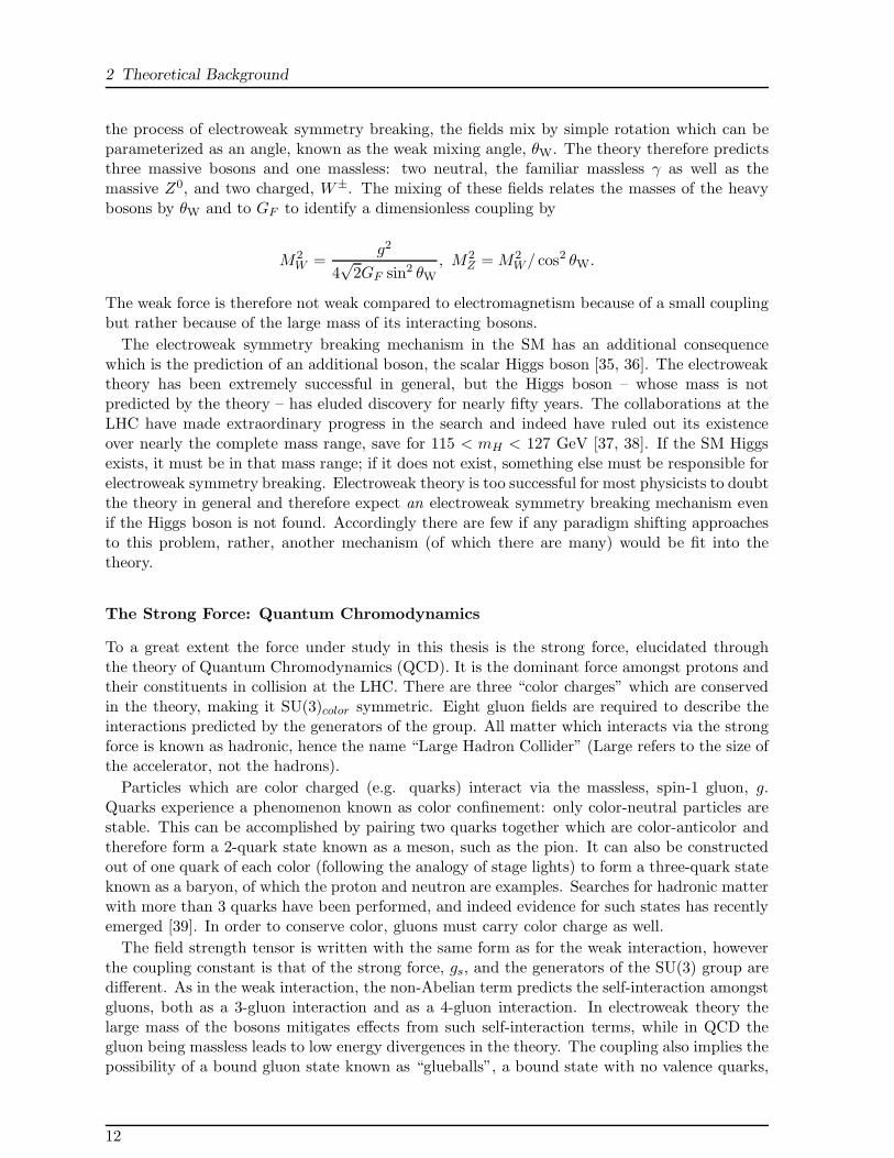
In 1995, the top quark was discovered by the CDF and DØ Collaborations at Fermilab’sTevatron in pair production [53, 54]. More recently, in 2009, both collaborations have observedthe production of a single top quark [55, 56], found to be consistent with SM expectations. Theprogress of the direct search limits and indirect SM constraints on mtop are shown over time inFigure 2.1, along with the early measurements at the Tevatron, consistent with expectations.The discovery of the top quark and the fact that its mass was found to be consistent with globalfits to data predicted it are true feats of the Standard Model.
Properties of the Top Quark
A wealth of measurements of top quark properties have been undertaken at the Tevatron, atradition which the LHC is continuing. At the time of writing the most precise measurementsof the top quark properties still come from the Tevatron, some of which will be discussed here.Top pair production cross section at the Tevatron will be discussed in the next section. A morecomplete review of property measurements can be found, for instance, in [21].
The top quark is expected to decay almost entirely as t→ Wb, since other quark flavor decaysare suppressed by tiny off-diagonal CKM Matrix elements and by larger mass differences. Thiscan be tested by measuring the ratio Rb, defined as Rb = Γ(t → Wb)/Γ(t → Wq), whereq = d, s, b. The ratio has been measured by both the CDF and DØ collaborations and combined(externally) to obtain [57, 58, 21]:
Rb = 0.99+0.09−0.08,
which is dominated by the more precise DØ measurement. Given that measurements of Rb
are consistent with 1, the top quark is assumed to always decay as t → Wb in this thesis. Themeasurement of Rb can be used as one of the inputs to measure the total width of the top quark,
14
2.2 The Top Quark
Year
Mt
[G
eV
]
SM constraintTevatron
Direct search lower limit (95% CL)
68% CL
50
100
150
200
1990 1995 2000 2005
Figure 2.1: The development of knowledge of the top quark mass over time. The black line isthe direct search limit, and the shaded area is the 68% confidence level for the mass based ona global fit of precision electoweak data interpreted within the SM. The actual measurementsfrom the first decade of the Tevatron’s measurements of the top quark, beginning in 1995, areshown. Image from [52].
Γtop, determined by DØ to be [59]:
Γtop = 1.99+0.69−0.55 GeV.
Using the uncertainty principle [60], this implies that the lifetime of the top quark is
τtop = 3.3+1.3−0.9 × 10⁻²⁵ s,
which is in agreement with theoretical predictions. The characteristic timescale of QCD canalso be calculated as well using ΛQCD, to be
τQCD = 3.1 ± 0.7 × 10⁻²⁴ s.
15

2 Theoretical Background
The fact that the lifetime of the top is shorter than the characteristic timescale of QCD meansthat it decays before hadronization, the only quark to do so. This preserves much information inthe final state which is generally lost for the lighter quarks [61]. This behavior has lent itself toextremely precise measurement of many of the top quark properties, in particular its mass. Thecurrent average of the top quark mass from Tevatron experiments ismtop = 173.2 ± 0.9 GeV [22].For practical purposes, the top quark is assumed to have a mass of mtop = 172.5 GeV throughoutthis thesis, and the cross section will be quoted as such.
Decay of the Top Quark and the tt Final State
These properties of the top quark have profound experimental significance. That the top quarkcannot hadronize before it decays combined with the fact that it decays into a W boson anda b-quark yields an extremely identifiable final state. In contrast to the top quark, b-quarksare relatively long lived; they hadronize and often travel a distance measurable in the detectorbefore decay. Independent how the W is produced, it can decay as either W → qq or W → lν.Excluding the third generation of quarks (mtop > mW), a W can decay hadronically into quarksof the first or second generation, ignoring CKM suppressed decays. These contributions are eachenhanced by a color factor of three since the weak force is colorblind. A leptonically decayingW can decay into all three generations. The branching ratio for each of these nine channelsis approximately equal, 1/9 ≈ 11 %. More precise numbers for the W branching ratio can befound in [21].
After the decay of tt, three possible combinations of W decay are named “all-hadronic” whenboth decay as W → qq, “dileptonic” when both decay as W → lν, or “semileptonic” when oneW decays hadronically and the other leptonically. A simple probability calculation shows thatthe all-hadronic channel is the most likely final state and the dilepton channel is the least. Thesemileptonic channel, which accounts for about 30 % of the decays of top quark pairs, is studiedin this thesis. It should be noted that the τ lepton decays further within the detector and isnot explicitly considered in these analyses. Accordingly, a decay chain like W → τν followed byτ → µν is considered as a leptonic W decay, though if the τ decays as τ → qq it is consideredhadronic.
2.3 Cross Section Predictions at Hadron Colliders
Precise predictions of cross sections at a hadron collider are a difficult task, though great strideshave been made in recent years. Knowledge of both the interactions at play and the structureof the proton are essential in this task. Cross section predictions generally done first as akinematically inclusive cross section before being calculated differentially. The latter is thenused in a MC generator to make kinematic predictions. Predictions for both top quark pairproduction cross section and W boson in association with jets will be discussed here.
Production Cross Section Calculations: The Main Idea
The effort of using a QFT in the SM to calculate for the cross section of a process is done bya perturbative expansion in coupling constant, technically achieved by using the Feynman rulesfor the interaction in question. In the case of quark pair production at the LHC, the strongforce is hugely dominant, so the interaction studied is QCD. A more complete explanation canbe found in [41], for instance.
16

2.3 Cross Section Predictions at Hadron Colliders
The process of deriving a production cross section begins with the probability for a quan-tum mechanical transition of state, described by Fermi’s Golden Rule, relating the transitionamplitude of a process to the sum of contributing matrix elements squared, |M|2, integratedover phase space. The perturbation expansion of QCD is used to approximate |M|2. The otheressential input to such a prediction is knowledge of the proton structure. Fermi’s rule relatesthe transition probability from a given state to another; in our case the final state desired isclear but the initial state is not.
The proton is composed of partons – quarks and gluons. At rest, the proton can be describedby comprising two u quarks and one d quark, known as the valence quarks. At low energies,the three valence quarks together carry about half of the proton’s longitudinal momentum. Asa proton is accelerated, what is known as the particle “sea” develops. The sea consists of lowpT partons which carry a fraction of the proton’s longitudinal momentum. As the energy isincreased, the sea partons carry more and more of the proton’s longitudinal momentum whilethe valence quarks carry less and less. More than fifty years of experimental research have leadto a decent understanding of the distribution of the fraction of energy carried by each partonin the energy range accessible at the LHC, known as the Parton Distribution Function (PDF).The fraction of longitudinal momentum carried by the interacting partons, denoted x for each,determines the effective energy of the collision.
The total cross section for the production of a pair of particles of mass m in a proton-protonprocess as a function of the center-of-mass collision energy
√s is
σm(√s) =
∑
i,j
∫
dx1dx2 σij(Q2,m2, µ2)f i
1(x1, µ, )fj2 (x2, µ).
The functions f i1 and f j
2 are the PDF for each of the two protons, the parton i from the firstproton carries a momentum fraction x1 and from the second parton j a fraction x2. Here, σ isthe partonic cross section for the process in question which is calculated by summing the squaresof the contributing matrix elements. The integral runs from a characteristic low scale, such asΛQCD, to the maximum which is kinematically permissible. Contributions below the integralbounds lie in a regime where perturbative QCD breaks down and are handled by the PDF.This is known as factorization, which is an essential tool in making predictions. The partonmomentum transfer in the collision is Q2 ≡ x1x2s. All partons considered in the PDF aresummed over. The theoretical maximum of Q2 is in s itself, if the parton from each proton inquestion happens to carry the full momentum of its proton, a very unlikely situation due to thedistribution of momentum amongst the partons. An example of a PDF is shown in Figure 2.2at two different Q values for the CTEQ6M set [62], similar to the PDF sets used in this thesis.The renormalization scale, µ, is essential for predictions but is not a physical parameter; σ(
√s)
should therefore in principle be independent of it, however in practice this is not the case. Thechoice of µ is arbitrary, but often taken by convention to be the mass of the particle in question.To asses any systematic uncertainty on a theoretical prediction caused by this choice, µ is oftenvaried by a factor of 2 up and down.
Inclusive Calculations
After making use of factorization, the parton cross section, σ, must be evaluated. Following[63], the threshold for production is introduced as a parameter, ρ ≡ 4m2/Q2, which is essentialin assessing the magnitude of contributions. The parton cross section σ for heavy quark pairproduction can be written as
17

2 Theoretical Background
Figure 2.2: The CTEQ6M parton distribution functions, showing the fraction of energy (x)carried by a specific parton type, from [62]. It is shown at two energies, Q= 2, 100 GeV. Onecan see that gluons dominate the PDF over most the range of x.
σ(Q2,m2, µ2) =α2
s(µ2)
m2fij(ρ,
µ2
m2),
where the functions fij correspond to the various contributing processes and i, j are the incomingpartons. An expansion around αs(µ
2) is therefore needed in order to calculate σ. The functionsfij can be expanded in (µ2/m2), as
fij(ρ,µ2
m2) = f0
ij(ρ) + 4παs(µ2)[
f1ij(ρ) + f1
ij(ρ) ln(µ2
m2)]
+O(α2s),
The functions f0ij are the leading order contribution for heavy quark pair production when
summed over initial state partons, f1ij is next to leading order (NLO), and so on. Keeping
in mind the equation is a part of the partonic cross section, the leading-order term in thecross section is of order α2
s as expected. Leading order production of a quark pair is by eitherquark-antiquark annihilation or by gluon fusion, shown in the Feynman diagrams in Figure 2.3.Calculations of such terms for heavy quarks were necessitated by the discovery of the massivecharm quark via observation of the cc bound state, the J/Ψ meson, in 1974 [64, 65]. The leadingorder functions f0
ij for heavy quarks were calculated a few years later [66, 67]. This was done
both as a function of Q2 and of mquark, therefore applicable not only to the original case-study ofcharm pairs in electron-positron annihilation but also to top pairs in proton collisons. It was thenestablished that both the gluon fusion and quark-antiquark annihilation processes contributedto cc production and therefore qq production for heavy quarks in general. At LHC energies, thegluon fusion process is expected to dominate over quark annihilation. In the expansion of fij,terms which are multiplied by a logarithm in µ2/m2 are gathered as fij, such that the NLOterm f1
ij shown. These terms are of higher order but are affected by a logarithmic factor andcan therefore be of more importance than other terms of the same order. Calculations of theseterms are often carried out in place of the full calculation at that order, known as the “leadinglog” approximation. Complete calculations at NLO (α3
s) were carried out in the late 1980’s [63].
18

2.3 Cross Section Predictions at Hadron Colliders
In the years since, approximate NNLO (α4s) calculations have become available for heavy quark
pairs in general and top quark pairs in particular [68, 69, 70].
Figure 2.3: The Feynman diagrams entering the matrix element calculation for QCD tt produc-tion in proton collisions at leading order. The two mechanisms are quark-antiquark annihilation(upper left) and gluon fusion (other three). The latter dominates at LHC energies.
The Top Quark Pair Production Cross Section
The predictions for the top quark pair production cross section currently available come in twoforms: an inclusive cross section and a differential cross section. In the analyses presented here,differential cross section predictions in the form of NLO MC is to model the kinematics of topquark pairs but the total cross section used for expectations is the best available approximateNNLO prediction. The MC simulation will be discussed more in Section 5.1. For inclusiveσtt, Hathor is used with the CTEQ6.6 PDF set [13, 62]. The renormalization and factorizationscales are taken to be mtop in both the MC simulation and the inclusive calculation. In the MCsimulation as throughout this thesis, mtop = 172.5 GeV is used. A prediction of
σtt = 164.6+11.5−15.8 pb
is taken to be the inclusive cross section for tt production in pp collisions at√s= 7 TeV.
The first measurements of σtt were performed at Fermilab’s Tevatron, a pp collider with acenter-of-mass energy of
√s = 1.8 TeV at the time. These first measurements by the CDF and
DØ collaborations accompanied the announcement of the discovery of the top quark [53, 54].They have since been refined to a much greater accuracy at
√s = 1.96 TeV. The latest and
most precise result measures σtt = 7.50 ± 0.48 pb from CDF in about 5 fb−1 of data, achievinga relative uncertainty of 6.4 % [71]. The DØ collaboration measures σtt =7.56+0.63
−0.56 [72]. Bothmeasurements agree with approximate NNLO QCD calculations for the process at the Tevatron,which predicts σtt = 7.46+0.66
−0.80 pb [71].In 2010, the ATLAS and CMS collaborations both published measurements of σtt in proton-
proton collisions at a center-of-mass energy of√s = 7 TeV in about 3 pb−1 of data [5, 6].
ATLAS measured σtt = 145+52−41 pb, a total uncertainty of 30-40 %. This served to establish the
signal at this energy and showed already that there are no enormous surprises in the rate oftt production. This measurement, along with the corresponding CMS measurement, is shown
19

2 Theoretical Background
in Figure 2.4 together with the measurements from the Tevatron at proton-antiproton collisionenergies of
√s = 1.8 and 1.96 TeV. The theoretical prediction for the dependence of σtt on the
center-of-mass energy for both types of collisions is shown as well. This essentially represents theknowledge of σtt at
√s = 7 TeV before the work presented in Chapters 7 and 8 was undertaken.
[TeV]s1 2 3 4 5 6 7 8
[p
b]
t tσ
1
10
210
ATLAS
)1(2.9 pb
CMS
)1(3.1 pb
CDF
D0
NLO QCD (pp)}
Approx. NNLO (pp)
)pNLO QCD (p
)pApprox. NNLO (p
6.5 7 7.5
100
150
200
250
300
Figure 2.4: The top pair production cross section as a function of center-of-mass collisionenergy, as of late 2010. Measurements from the Tevatron at pp collision energies
√s = 1.8
and 1.96 TeV are shown along with the results from the very first 3 pb−1 of data from LHC ppcollisions at
√s = 7TeV. The error bars on the measured σtt values represent the sum of all
uncertainties. Theoretical predictions shown are from Hathor[13], with the uncertainty bandcorresponding to scale and PDF uncertainties.
The Production of W+jets
The production of a W boson with associated jets yields the same final state objects as in thedecay of top quark pairs. The predictions for the cross section of this process are significantlymore complicated because it is higher order in αs, often involving more partons in the matrixelement calculation. Since two of the analyses in this thesis make use of the assumption thatevery top quark decays as t → Wb, the production of W+jets where one or two of the jets arefrom heavy quark decays is of importance.
The basic process for W production is qq′ → W and yields only the direct decay productsof the W in the final state. The LO Feynman diagram is shown in Figure 2.5, together witha contribution to the W+1 jet final state. Leading order predictions for the W/Z+2 jets crosssection were first completed in the mid-1980’s and by now W+4 jets is available at NLO [73, 74,75]. The LO to NLO k-factor corrections for W+jets are in the range of 1.5-2.0 [75], motivatingboth the need for special experimental care and for more precise calculations. In the analyseshere, the W+jets contribution will be determined in each jet bin separately, with a constraint of
20

2.3 Cross Section Predictions at Hadron Colliders
∆σ ∼ 50%, however the kinematics used to describe it will be LO as no higher order simulationis available as of yet.
Figure 2.5: The LO Feynman diagram for exclusive W production in proton-proton collisionswhich is from quark annihilation (left), together with an example of initial state gluon radiationoff of one of the incoming quarks, a LO contribution to the W+1-jet final state (right).
The final states of particular interest in such calculations areW plus a heavy quark pair, W+bband W+cc, as well as W plus a single heavy quark, W+b/b and W+c/c. These are calculated asan N -jet final state where one or two of the jets is heavy flavor. The main contributing Feynmandiagrams are shown in Figure 2.6 [76]. The calculations for either b or c in the final state arequite similar in principle.
Figure 2.6: The dominant Feynman diagrams for W production in association with heavy-flavor jets, where Q = c, b. The dominant mechanism for heavy flavor pair production is aradiated gluon splitting to QQ (top left). For single production of a heavy flavor jet, the mainmechanisms are either a heavy parton directly from the PDF (top right) or a flavor-changingweak current to produce the heavy flavor quark along with the W (bottom row). The latterdominates for W + c production, with an s-quark in the initial state. The PDF contributiondominates for W + b production due to CKM suppression of the s → Wb vertex and the as ofyet immeasurably small top quark component of the proton PDF. Initial and final state gluonradiation in any of these processes can produce additional jets.
There are two mechanisms to produce of a single heavy quark jet: there is either a flavorchanging (weak) current to produce both the W and the heavy quark or there is a heavy partonin the initial state. The LO Feynman diagrams for these two processes are shown in Figure 2.6.
21

2 Theoretical Background
The production of charm is enhanced with respect to bottom due to the strange componentof the PDF, where the process sg → Wc is favored due to Vcs in the CKM matrix [77]. Bycomparison, production of a b-quark in the final state by the same mechanism would require atop quark in the PDF, a process so thoroughly negligible it is not considered. A s→Wb vertexis therefore necessary for that process to produce a single b-quark, which is CKM suppressed.The main contribution to the production of a b-quark in association with a W is thereforeexpected to contain a b-quark coming directly from the PDF. The large b mass suppresses thiscontribution from the PDF as well.
The prediction of W + c has begun to reach NLO accuracy. Results show that it is a non-negligible portion of the inclusiveW+jets production cross section[76]. Interest in the suppressedW + b is in great part due to the recent observation of single top quark production which hasthe same final state [55, 56], making W + b an essential background to understand for thatmeasurement, if of a small magnitude. Indeed the process has been measured by ATLAS andfound to have a central value larger than expected but consistent with predictions nonetheless [78,79].
The main mechanism for heavy quark pair production in association with a W comes fromgluon splitting, g → QQ [80]. These predictions for W+bb and W+cc have reached NLOprecision [81, 80, 82]. There is particular interest in W+bb due to the possibility to observe aHiggs boson in the H → bb decay channel, where a Higgs is produced along with a W . Thiswould lead to W+bb final state as well, making direct production of W+bb a background to theHiggs search in this final state, thereby necessitating its precise prediction [80].
In the analyses presented here, most processes are normalized to theoretical predictions, whilesome are normalized to measurements from within ATLAS where available. The W+jets back-ground and in particular the heavy flavor content is normalized to measurements. In general,the heavy flavor content is treated as a ratio of events containing a certain jet configuration inthe final state to all other jet configurations, as found in the MC.
To quantify the heavy flavor content in data with respect to the MC, the ratio fWHFis defined,
such that
fWHF·(
σ(W+QQ)incl.
σ(W+2 jets)incl.− σ(W+QQ)incl.
)
MC
=
(
σ(W+QQ)incl.
σ(W+2 jets)incl.− σ(W+QQ)incl.
)
Measured
,
where Q = b, c. The denominator has all 2-jet (inclusive) configurations except for the processesconsidered in the numerator, which are those containing a pair of heavy flavor jets. A valuefWHF
= 1 is therefore the expectation before measurement. It should be noted that the W + bprocess is technically included in the numerator of the definition, although only the contributionwith a PDF b-parton is considered3. The process is mathematically assumed to scale with W+bband W+cc, but no physical sensitivity to the process expected.
Similarly, fWc is defined, such that
fWc ·(
σ(W+c/c+jet)incl.
σ(W+2 jets)incl.− σ(W+c/c+jet)incl.
)
MC
=
(
σ(W+c/c+jet)incl.
σ(W+2 jets)incl.− σ(W+c/c+jet)incl.
)
Measured
.
Note that the denominators are not the same in the definition of fWHFand fWc; in the former
case the W + c process is included while W + bb and W + cc are excluded, and vice-versa.
3This process with a PDF b-parton is so small that it is not even mentioned whether or not it is indeed simulatedin the manual for the MC generator used, ALPGEN [83, 84]. The author of the generator claims, however,that it is calculated. The other processes, which require a flavor-changing interaction, are found in ALPGENfor c-quarks but not b-quarks, because the author ‘didn’t think it would have a large cross section’.
22

2.3 Cross Section Predictions at Hadron Colliders
The analysis in Chapter 7 is flavor-sensitive and treats the uncertainty on fWHFand fWc as a
systematic uncertainty in the determination of σtt. The analysis in Chapter 8 is almost entirelyinsensitive to flavor effects. For the final analysis presented in Chapter 9, the fractions fWHF
and fWc are measured simultaneously with σtt.
23

Large Hadron Collider. “When charged particles of more than 5 TeV pass through a bubblechamber, they leave a trail of candy.”[19]
3 Experimental Environment
The data analyzed in this thesis are high energy proton-proton collisions produced by he LargeHadron Collider (LHC) and recorded by the ATLAS detector, at CERN in Geneva, Switzerland.The accelerator and the detector will both be described here.
3.1 The LHC Accelerator
The LHC is a proton-proton (pp) collider which began successful operation in autumn 2009,and has been improving its performance since. The LHC is 27 km in circumference, built in thetunnel originally used by the LEP collider, about 100 m below the surface of the earth in thebedrock of the Alps. Four main experiments are built in caverns at the level of the accelerator,each one at an interaction point where the beams of protons are brought into collision. Eachbeam consists of huge numbers of protons, organized first into “bunches” – about 1011 protons,packed as densely as possible – spaced at intervals of 50 ns [85] (about 15 m). These bunchesare organized into “trains”, which are groups of bunches, typically 8 or 12 bunches long during2011. The trains are separated by a longer distance from one another. A theoretical maximumof 2,808 bunches in the LHC at once is possible, which would require a spacing of only 25 ns[85].So far, a maximum of 1,380 – the maximum with 50 ns spacing – has been achieved[86].
Protons being accelerated go through a chain of many steps, beginning with a bottle ofhydrogen gas and ending with the LHC [85]. Hydrogen molecules are dissociated in an electricfield, breaking H2 into hydrogen atoms and stripping the electrons away. A magnetic field isapplied to bend the positively charged H+ (that is, the proton) in the direction opposite fromthe electrons. The protons are accelerated in a linear accelerator up to 50 MeV, then injectedinto the Proton Synchrotron Booster (PSB), which subsequently accelerates protons to 1.4 GeV.They are then accelerated up to 450 GeV in the Super Proton Synchrotron (SPS) after passingthrough the 25 GeV Proton Synchrotron (PS) accelerator. At an energy of 450 GeV, protons areinjected into the LHC, where they are accelerated to their final collision energy.
The LHC has 1,232 bending dipoles which make up the core of the accelerator, as well as asystem of quadrupole, sextupole, and octupole magnets used to bring the proton beams intocollision at the interaction points, at the center of each detector. The LHC’s accelerator chainis shown in Figure 3.1. At the time of writing, the LHC has operated in three stages of energy:first at 450 GeV per beam, then at 1.18 TeV, and finally an operational energy of 3.5 TeV. Alldata analyzed in this thesis are recorded at 3.5 TeV per beam, providing a center-of-mass energyof
√s= 7 TeV. A visualization of the very first collision event recorded by ATLAS, at
√s =
900 GeV, is shown in Figure 3.2 alongside one of the first di-jet events recorded by ATLAS at√s= 7TeV, four months later.
The LHC can also be used as a heavy ion accelerator for lead ion collisions, where each nucleonpresent achieves the highest energy deliverable by the accelerator, so far 3.5 TeV / nucleon. Giventhe density of a bound nucleus, an ion beam brought to these energies behaves very differentlyin collision than bunches of protons, allowing for study of low-pT, high multiplicity events (incontrast to the proton physics program, which focuses on the opposite). The heavy-ion physics
25

3 Experimental Environment
Figure 3.1: The CERN accelator complex, including the LHC. The trajectory of a proton canbe followed from the LINAC to the Booster and PS, then on to the SPS and finally the LHC.Image from [87].
Figure 3.2: The first collision provided by the LHC recorded by the ATLAS detector, at√s=
900 GeV, on 23 November 2009 (left). Soft hadronic activity can be seen. di-jet event recordedby ATLAS during the first
√s= 7 TeV collision fill on 30 March 2010 (right). Images from [88]
and [89].
program at the LHC has proved successful, both for the special-purpose ALICE detector designedprecisely for heavy ion collisions and for the multi-purpose detectors, CMS and ATLAS.
26

3.1 The LHC Accelerator
Day in 2010
24/03 21/0419/05 16/06 14/07 11/0808/0906/10 03/11
]1
s2
cm
30
Pe
ak L
um
ino
sity [
10
0
50
100
150
200
250 = 7 TeVs ATLAS Online Luminosity
LHC Delivered
1 s2 cm32
10×Peak Lumi: 2.1
Day in 2011
28/02 02/0405/05 08/06 11/07 14/08 16/0920/10 22/11
]1
s2
cm
33
Pe
ak L
um
ino
sity p
er
Fill
[1
0
0
0.5
1
1.5
2
2.5
3
3.5
4
4.5 = 7 TeVs ATLAS Online Luminosity
LHC Stable Beams
1 s2 cm33
10×Peak Lumi: 3.65
Figure 3.3: The peak instantaneous luminosity delivered to ATLAS by the LHC in 2010 (left)and 2011 (right). One can see a clear increase over time, as the LHC improved its performance.The y-scale on the right plot is three orders of magnitude higher than on the left plot. Imagesfrom [90].
Proton Beam Data Delivered at√s = 7 TeV
To quantify the amount of data delivered by a collider, the instantaneous luminosity L is defined,a measure of particle flux from two sources per unit time:
L = fnN1N2
Acm−2 s−1.
Here, N1 and N2 are the number of particles in each bunch, n is the number of bunches ineach beam, f is the revolution frequency and A is the cross-sectional area of the beams. Peakluminosities on the order of ∼ 1033 cm−2 s−1 have already been achieved at the LHC, just oneorder of magnitude lower than the design [85, 90]. The time-integrated luminosity,
∫
L dt, hasthe units of inverse cross-section, and indeed is directly proportional to the number of events(N) expected for a given physical process, by a factor of the cross section σ:
N = σ ×∫
L dt.Measuring the cross section σ of the tt process is the goal of this thesis, and the uncertainty
on the measurement goes down with an increasing amount of data (for a simple counting exper-iment the statistical uncertainty goes as
√N , thus the relative uncertainty goes as 1/
√N). It
is therefore in the interest of such measurements to collect more luminosity, and, in the interestof time, the highest instantaneous luminosity possible. Given that the accelerator has alreadybeen built – defining the revolution frequency and the cross-sectional area of the beams – lumi-nosity can be increased by stuffing more protons into a given bunch, putting more bunches intothe accelerator at once and by running for a longer time. The peak instantaneous luminositydelivered to ATLAS as a function of the day in both 2010 and 2011 is shown in Figure 3.3, andthe integrated luminosity delivered by the LHC to ATLAS and recorded by ATLAS is shown inFigure 3.4. One can see there increasingly higher peak instantaneous luminosities, an effect ofboth adding bunches over time and adding protons to each bunch. Work has been done in orderto calibrate the measurement of the integrated luminosity recorded by ATLAS and to estimateits uncertainty [91, 92]. An uncertainty of 3.4 % on its magnitude is used for 2010, with a slightlyincreased uncertainty of 3.7 % in 2011.
27

3 Experimental Environment
Day in 2010
24/03 19/05 14/07 08/09 03/11
]1
To
tal In
teg
rate
d L
um
ino
sity [
pb
0
10
20
30
40
50
60
Day in 2010
24/03 19/05 14/07 08/09 03/11
]1
To
tal In
teg
rate
d L
um
ino
sity [
pb
0
10
20
30
40
50
60 = 7 TeVs ATLAS Online Luminosity
LHC Delivered
ATLAS Recorded
1Total Delivered: 48.1 pb1
Total Recorded: 45.0 pb
Day in 2011
28/02 30/04 30/06 30/08 31/10
]1
To
tal In
tegra
ted L
um
inosity [fb
0
1
2
3
4
5
6
7 = 7 TeVs ATLAS Online Luminosity
LHC Delivered
ATLAS Recorded
1Total Delivered: 5.61 fb1Total Recorded: 5.25 fb
Figure 3.4: The integrated luminosity delivered to ATLAS by the LHC and recorded byATLAS, both in 2010 (left) and 2011 (right). The amount of data recorded has grown rapidlyover time since the LHC has begun delivering pp collisions. The y-axis of the plot on the right isthree orders of magnitude larger (units of fb−1) than that of the left-hand plot (pb−1). Imagesfrom [90].
Day in 2010
24/03 19/05 14/07 08/09 03/11
Pe
ak <
Eve
nts
/BX
>
0
0.5
1
1.5
2
2.5
3
3.5
4
4.5 = 7 TeVs ATLAS Online
LHC Delivered
Day in 2011
28/02 30/04 30/06 30/08 31/10
Pe
ak A
ve
rag
e Inte
ractio
ns/B
X
0
5
10
15
20
25 = 7 TeVs ATLAS Online
LHC Delivered
Figure 3.5: The peak of the average number of interactions per bunch crossing, < µ >, shownper luminosity block (60 or 120 s of data taking) as a function of time in 2010 (left) and 2011(right). One can see clearly how this is correlated with the instantaneous luminosity, shown inFigure 3.3. Images from [90].
Increasing instantaneous luminosity does however come with an experimental challenge, knownas “pileup”. The interaction of partons in a proton-proton interaction is a statistical process,whose chance of occurring is increased by increasing the number of protons present. Nothingprevents several parton-parton interactions from occurring in one crossing of the proton beams,indeed such “multiple interactions” are the norm. The average number of parton interactionsper bunch crossing, < µ >, is shown for the data recorded in 2010 and 2011 in Figure 3.5. Theexperimental challenges this poses will be discussed in Section 4.1.
28

3.2 The ATLAS Experiment
3.2 The ATLAS Experiment
The ATLAS (A Toroidal LHC ApparatuS) detector is one of the two multi-purpose detectorsat the LHC. It is located at interaction point 1, just across the street from the main entranceto CERN. ATLAS is built following a “traditional” detector design, with an inner trackingdetector to measure charged particle’s trajectory, followed by calorimeters to measure bothelectromagnetic and hadronic interactions, all surrounded by a designated muon tracking system.A schematic view of the entire detector can be seen in Figure 3.6. The outer muon system alsoresides in a magnetic (toroidal) field that has eight-fold symmetry around the beam pipe. Asmaller toroidal magnetic system, also with eight-fold symmetry and staggered with respect tothe barrel magnets, is used for the outermost regions of ATLAS. The complete design of theATLAS detector is laid out in [93, 94].
Figure 3.6: A schematic view of the ATLAS detector. From inside to out, the inner detector ismade up of the pixel detector, the SCT, and the TRT, which reside in a 2 T solenoidal magneticfield. The various calorimeter systems (LAr and Tile) are found beyond that. The outermostlayer of the detector is the muon system, present both in the barrel region and making up thetwo “wheels” beyond the main body of the detector, situated in a toroidal field. Image from [95].
Coordinate System
The ATLAS detector uses a right-handed coordinate system. The +x direction points fromthe interaction point towards the center of the LHC, while the +y direction points skywards.The beam travels along the z-axis, making the x-y plane transverse to it. Most often, polarcoordinates are used. The azimuthal angle φ is measured in the x− y plane, where transversekinematic definitions including transverse momentum (pT), transverse energy (ET), and missingtransverse energy (Emiss
T ) are defined. The rapidity angle θ is defined as the angle from thebeam axis, and the pseudorapidity η, defined as
η ≡ − ln tan(θ/2),
29

3 Experimental Environment
is generally used. A very useful quantity for measuring the distance between two objects in thedetector, ∆R, is defined as
∆R ≡√
∆φ2 + ∆η2.
Two different coordinate system definitions are used, “detector” and “physics”. In detectorcoordinates, the physical center of ATLAS is taken to be the origin of coordinates. Objectselection is based on the physical limitations of the detector and therefore uses the detectorcoordinate system. In physics coordinates, the reconstructed primary vertex of the event istaken to be the origin of coordinates. Higher order corrections to reconstruction, such as anobject’s pT, are often taken into account using physics coordinates. It should be noted, however,that the beam spot of the LHC is significantly more accurate in z than it was at the Tevatron,making the distinction between physics and detector coordinates less critical than there.
Inner Detector
The ATLAS inner detector is designed to precisely reconstruct the trajectory of charged par-ticles in a 2T solenoidal field over a range of hundreds of MeV to a couple of TeV [95]. Theextremely precise pixel detector is closest to the beamline is, followed by the silicon strip tracker(SCT). This is in turn surrounded by the transition radiation tracker (TRT), a dedicated systemfor distinguishing pions from electrons. The inner detector covers up to |η| < 2.5, making itphysically about 7 m long and 2.3 m in diameter. A plan view of one quadrant of inner detectorcan be seen in Figure 3.7.
Envelopes
Pixel
SCT barrel
SCT end-cap
TRT barrel
TRT end-cap
255<R<549mm|Z|<805mm
251<R<610mm810<|Z|<2797mm
554<R<1082mm|Z|<780mm
617<R<1106mm827<|Z|<2744mm
45.5<R<242mm|Z|<3092mm
Cryostat
PPF1
CryostatSolenoid coil
z(mm)
Beam-pipe
Pixelsupport tubeSCT (end-cap)
TRT(end-cap)
1 2 3 4 5 6 7 8 9 10 11 12 1 2 3 4 5 6 7 8
Pixel
400.5495
580
650749
853.8934
1091.5
1299.9
1399.7
1771.4 2115.2 2505 2720.200
R50.5R88.5
R122.5
R299
R371
R443R514R563
R1066
R1150
R229
R560
R438.8R408
R337.6R275
R644
R1004
2710848712 PPB1
Radius(mm)
TRT(barrel)
SCT(barrel)Pixel PP1
3512ID end-plate
Pixel
400.5 495 580 6500
0
R50.5
R88.5
R122.5
R88.8
R149.6
R34.3
Figure 3.7: A plan view of one quadrant of the inner detector, with an enlargement of thepixel detector on the bottom. From inside to outside, the inner detector consists of the PixelDetector, SCT, and TRT, all residing in a 2T solenoidal magnetic field. Image from [95].
The pixel subsystem is at the core of the ATLAS detector. Each pixel sensor is a 50×400 µm2
chip, with a total of 80.4 million readout channels in the entire system. The pixel detector is laid
30

3.2 The ATLAS Experiment
out in three concentric layers in the barrel region, with three endcaps on either side. The designis such that a charged particle should always cross three layers of the pixel detector, aiding inprecise reconstruction of the track’s trajectory and offering redundancy in case of a hardwarefailure. In particular, the system is used in determining the location of a track’s vertex, usefulin distinguishing primary vertices from secondary. The closest layer, known as the b-layer, isabout 50 mm from the interaction point, just outside the beam pipe’s vacuum. As the namesuggests, it is designed to be able to identify the path of charged particles precisely enough toreconstruct the displaced decay vertex of a long-lived hadron, resultant from the production ofa b-quark in a hard interaction. The pixel detector’s calibration and functioning is crucial to theb-tagging algorithms which will be discussed in Section 4.4. Since there is very little materialin between the interaction point and the b-layer, it is also extremely useful for distinguishingelectrons from photons. The latter can convert in the detector, often after passing through theb-layer without leaving a hit there. Early measurements of the material in the pixel system andbeampipe, as well as particle energy loss per unit length, are shown in Figure 3.8.
The SCT system is a silicon strip detector, arranged with a geometry similar to that of thepixel system, covering a physically larger area to have the same η coverage. It is made up ofabout 6.3 million channels. The silicon strip technology is less precise than the digital pixelsystem but also significantly less expensive, allowing it to cover a larger area. A typical promptlepton track will have at least five hits in the SCT. Together with the pixel detector, these twosilicon detectors allow for precise track reconstruction.
The TRT surrounds the SCT with |η| < 2.0. It consists of about 300,000 drift tubes, 36 ofwhich should be crossed by most particles. While so many hits are in general useful for refiningtracking in general, it is dedicated to distinguishing electrons from hadrons (pions in particular).The high-threshold hits in the TRT signify photons radiated by an electron as it crosses fromone material to another, allowing for this discrimination. The three inner detector subsystemstogether allow for precise tracking of charged particles in general as well as measuring crucialproperties which aid the separation of certain types of particles from others.
Calorimeters
The ATLAS calorimeter is a set of several systems designed to be optimal for object reconstruc-tion over a very wide momentum range, from tens of MeV to a few TeV [98, 95]. Generally, thereis an inner electromagnetic (EM) calorimeter and an outer hadronic calorimeter. All componentsare sampling calorimeters. Calorimetry begins just after the inner detector’s solenoid.
The EM calorimeter is a lead-liquid-argon design (LAr), extending out to |η| < 3.2, with apresampler (PS) in the range |η| < 1.8 [95]. The granularity of barrel EM calorimeter reaches afineness of 0.003 × 0.01 (∆η × ∆φ) in the first of the three samplings (excluding the PS) and0.025× 0.025 in the second. The granularity of the EM endcap changes over η, with its finestgranularity the same as the barrel’s first sampling. A schematic of the highly efficient accordiondesign of the calorimeter is shown in Figure 3.9.
The barrel of the hadronic calorimeter consists of plastic scintillators in iron absorber plates(Tile) within |η| < 1.7. The first of the two out of thrsee samples have a granularity of 0.1× 0.1while the third is coarser in η, ∆η = 0.2. The hadronic calorimeter endcaps are again LArtechnology due to the radiation hardness necessary to be robust against increased particle flux,covering 1.5 < |η| < 3.2. The granularity is 0.1× 0.1 for 1.5 < |η| < 2.5, and 0.2× 0.2 for2.5 < |η| < 3.2. The forward calorimeters cover the outermost range, 3.1 < |η| < 4.9, with agranularity of 0.2× 0.2, following again the LAr technology.
31

3 Experimental Environment
p (GeV)2.5 2 1.5 1 0.5 0 0.5 1 1.5 2 2.5
)2
cm
1d
E/d
x (
Me
V g
0
1
2
3
4
5
6
7
8
9
10
1
10
210
310
410
510ATLAS PreliminaryGood Pixels>=3
Figure 3.8: Early measurements using the pixel detector. The reconstructed position of sec-ondary vertices in very early data, reflecting the material present (left). Image from [96]. Viewingfrom outside inwards, one can see the three layers of the the pixel detector, and then the beampipe itself. The stopping distance of particles is shown as a function of their momentum (right),from [97]. The various “stripes” in the plot correspond to different particles.
Muon System
The ATLAS muon system uses several different types of chambers, in particular two types withfast readout and coarse granularity used for triggering and two types with slower readout andfiner resolution for precision muon tracking [95]. The Monitored Drift Tubes (MDT) are theprecision chambers over much of the system, while Cathode Strip Chambers (CSC) are used inthe highest-radiation setting. The precision chambers cover up to |η| < 2.7, where the innermostchambers in the region 2.0 < |η| < 2.7 are CSCs and the rest are MDTs. The muon triggersystem uses Resistive Plate Chambers (RPC) in the barrel region up to |η| < 1.05 and ThinGap Chambers (TGC) in the endcap region, covering 1.05 < |η| < 2.4.
The Muon system sits in a toroidal field with a maximum bending power of 7.5 Tm perpen-dicular to the muon trajectory. Three toroids are used, each of which consist of eight coils,arranged symmetrically around the beam axis. Two of the toroids are for the endcaps, rotatedat 22.5◦ with respect to the barrel toroid, shown in Figure 3.9.
Trigger and Data Acquisition
The trigger system in ATLAS decides in near-real time (“online”) whether or not to record agiven event. It is designed in three levels which have access to increasing amounts of information,known as Level 1 (L1), Level 2 (L2), and the Event Filter (EF) [95]. Overall, the rate is reducedto 2-300 Hz, from its initial rate which changes depending on the accelerator’s conditions (theLHC’s design a ∼1GHz collision rate). The L1 trigger system runs on hardware distributedthroughout the detector, using coarse-grained information from specific systems: the dedicatedmuon trigger chambers, specific sections of the calorimeter, and parts of the SCT. In runningits algorithm, the L1 trigger identifies “Regions of Interest” (RoI) in η × φ where a potentialphysical object is present. The L1 trigger passes ∼ 100 kHz events to centralized L2 software,
32

∆ϕ = 0.0245
∆η = 0.025
37.5mm/8 = 4.69 mmm∆η = 0.0031
∆ϕ=0.0245x436.8mmx
Trigger Tower
∆ϕ = 0.0982
∆η = 0.1
16X0
4.3X0
2X0
1500 mm
470 mm
η
ϕ
η = 0
Strip cel l s in L ayer 1
Square cel l s in
L ayer 2
1.7X0
Cells in Layer 3
∆ϕ×∆η = 0.0245×0.05
Cells in PS
∆ϕ×∆η = 0.025×0.1
TriggerTower
=147.3mm4
Figure 3.9: Elements of the ATLAS detector design. The electromagnetic calorimeter’s ac-cordion design (left). The design of the ATLAS magnet system is shown (right). The innercylinder is the solenoidal magnetic in which the inner detector sits. The muon system’s barreltoroid surrounds that, and a smaller toroid for the muon endcap system (the “wheels”) can befound on either end. Images from [95].
which uses full detector readout for the RoIs in reconstruction algorithms which are simplifiedwith respect to those run offline. This is done in order to better determine whether or not aphysical object is indeed present. Several kHz of events pass the L2 selection for processingby the EF. The EF runs the full ATLAS reconstruction software in the online environment inorder to fully reconstruct the event. This is time intensive but has the advantage of being nearlyidentical to the algorithms used in a physics analysis. The EF chooses 2-300 Hz of events to bewritten out for permanent storage, to be considered for analysis.
The data acquisition system of the experiment is intertwined with the trigger system. Theheart of the data acquisition (DAQ) system are the Readout Drivers (RODs), which are sub-detector specific but are used throughout ATLAS [95]. RODs are essentially the detector readoutelectronics, which do their job after an L1 trigger accepts an event, and function as a buffer tohold the data throughout the process of the trigger decision. The RODs send information fora given RoI to the L2 trigger upon its request, and, if selected, send the information on to theEF. In the calorimeter, front end boards (FEB) perform the analog to digital signal processingnecessary before sending information onwards.

3 Experimental Environment
Snow Tracking. “I suppose that’s more accurately a hare dryer.”[19]
34
4 Reconstruction and Definition of Physical
Objects
The association of primary measurements in the detector with physical objects is describedhere, a process applied identically to the MC simulation and the data. Imperfect simulationcan give rise to discrepancies, which are understood and calibrated as best as possible. Thereconstruction process and the associated systematic uncertainties in analyses are discussed.
The selection of events is described here as well. There are two main steps in the selectionprocedure. The first is to determine which events can be considered for analysis at all: thosewhich have been triggered by an appropriate object and those in which we expect to have objectsthat can be well reconstructed. This is discussed in Section 4.1. Once an event is deemed tobe analyzable, the objects present in the event are reconstructed and selected as described inSection 4.2. Special attention is paid to the b-tagging algorithms used for identifying heavy-quarkhadrons in Section 4.4, which will be later used in Chapters 7 and 9.
For a tt pair which decays semileptonically, the end of the decay chain is two b-quarks, twolight quarks, an electron (e) or muon (µ), and a neutrino. Quarks are not observed directly butare reconstructed as jets, and the neutrino is not measured directly but quantified in terms ofmissing transverse energy in the event, Emiss
T . The selection of events from the recorded datasample reflect the expectation of observing a final state consistent with the semileptonic decayproducts of a pair of top quarks. The lepton flavor is used to classify events into lepton channels,called either “e+jets” or “µ+jets”. There are certain differences between the requirements inthe two channels, which will be noted.
Not all semileptonic tt events are observed; the efficiency of observation is modeled with MCsimulation which will be described in the next chapter. If a charged lepton is not observedthe event is not used. The expectation of four jets in the final state means that it is notimprobable for one jet to be lost. Furthermore, radiation effects mean that it is not unlikely foran additional jet to be observed. Accordingly, the analyses are further divided in “jet multiplicitybins”, according to the number of jets present in the event. The analyses in Chapters 7 and 8 usethe 3-jet exclusive bin, 4-jet exclusive bin and 5-jet inclusive bin, while the analysis in Chapter 9adds the 2-jet bin but uses the 4-jet bin inclusively.
This thesis contains analyses using two separate datasets, one recorded in 2010 totaling∫
L dt= 35 pb−1 and one recorded in 2011 comprising∫
L dt = 0.7 fb−1. Accordingly, certainconditions differing the data between the datasets, which require small changes to event andobject definitions. Unless otherwise noted, the statements apply equally to both lepton channelsin both datasets.
4.1 Event Level: Data Streams, Triggers, and Event Cleaning
In order to ensure that events considered are those in which proper reconstruction of physicalobjects can be done, a handful of event-wide requirements are put in place.
35

4 Reconstruction and Definition of Physical Objects
Good Run List
The main work of requiring that an event can be considered for analysis is done by the GoodRun List (GRL) mechanism, which is applied to all recorded data events in order to preselectthose in which protons are being collided and the entire detector is performing as expected.An example of a situation where an event would not be considered is if a crucial section of thedetector has been temporarily switched off due to a high-voltage trip. Good data quality forall relevant detector subsystems is required (those described in Section 3.2, with the generalexception of calorimetry beyond |η| > 2.5). Additional checks ensure that each type of physicalobject needed in the analysis is well behaved in the data, also included in the GRL. Becauseof the necessity to veto a second lepton, the muon channel analysis must always be able toreconstruct electrons and vice-versa.
Trigger
A trigger is required to fire for an event to be recorded by the detector, as described in Section 3.2.A balance must be found between the bandwidth available to the detector and the requirementsfor the physics analysis. The expectation of a lepton present in the event provides a cleantrigger (as opposed to jets, for instance, which pose enormous experimental challenges. See forinstance [99]). The lowest possible thresholds and quality are used at every turn, for two reasons.Foremost, the algorithms run online for the trigger are not identical (at L1 in particular) to thoserun in the full “offline” reconstruction for the analysis; having a looser selection at the triggermeans that more events will be available to the offline algorithms, thereby increasing efficiencyin the turn-on region. The best example of this is the pT of the object, for which a triggerhas a turn-on. A 15 GeV electron trigger will be fully efficient for offline electrons by about18 GeV, due to the differences in the algorithms. Furthermore, looser criteria in the definitionof the online object is necessary for the methods used to estimate the contributions due to fakeleptons, to be discussed in detail in Chapter 5. In general, looser requirements online mean ahigher rate of triggered events.
As the LHC delivered higher and higher instantaneous luminosity throughout the periodsanalyzed here, the trigger requirements had to be tightened. Several triggers have been useddepending on when the data was taken, all of which have thresholds for both quality and pT
sufficiently lower than the leptons in the analysis at hand. Of note is that the electron triggerrate for the last trigger used in 2010 was predicted to be too high for the 2011 conditions,necessitating raising the trigger threshold from 18 to 22 GeV. The offline cut in the analysis wasadjusted accordingly. All triggers used for µ are in their efficiency plateau by pT>20 GeV. Atrigger simulation in the MC is used, and it is required to have been fired for MC events aswell. Small differences between the simulation of the trigger and its real performance have beenobserved, giving rise to a systematic uncertainty discussed for each lepton separately.
Calorimeter Cleaning
Two phenomena which affect the calorimeter have occured which affect reconstruction capabil-ities; these are not accounted for by the GRL. Non-physical high-energy bursts in individualcells in the electromagnetic calorimeter have been observed. These bursts cause a “jet” to bereconstructed and greatly affect the Emiss
T calculation. Events in which such a burst occurred areidentified by requiring a certain “quality” of all jets, by checking the timing associated with it,fractions of energy found in the EM versus hadronic calorimeter, and other such sanity checks.If any jet with pT> 10 GeV in an event fulfills the criteria signifying that it came from such a
36

4.1 Event Level: Data Streams, Triggers, and Event Cleaning
(e)ϕ3 2 1 0 1 2 3
Eve
nts
/ 0
.31
0
5000
10000
15000
20000
25000 = 7 TeVsData 2011,
tt
W+Jets
QCD Multijet
Z+Jets
Single Top
Diboson
1 L dt = 0.7 fb∫
e+ 1 Jet
(leading jet)η2.5 2 1.5 1 0.5 0 0.5 1 1.5 2 2.5
Eve
nts
/ 0
.50
0
20
40
60
80
100
120310×
= 7 TeVsData 2011,
tt
W+Jets
QCD Multijet
Z+Jets
Single Top
Diboson
1 L dt = 0.7 fb∫+ 1 Jetµ
Figure 4.1: The gap caused by the death of 6 adjacent calorimeter front end boards in run180614, affecting 75% of the
∫
L dt = 0.7 fb−1 dataset. The left-hand plot shows the φ ofelectrons in the e+jets channel, showing a clear dip in the region -0.64 < φ <-0.74. The right-hand plot shows the reconstructed jet η in the µ+jets channel, showing a slight asymmetrycaused by the jet veto in 0 < η < 1.4. Both plots use the 1-jet inclusive selection which will bedescribed in this chapter.
burst, the event is discarded. This requirement is applied only to data and is considered to notrequire adjustment in the MC due to the very low rate of these bursts.
A plague of dying FEBs has affected the calorimeter, making the data inaccessible. Twoseparate mechanisms have been put in place to handle this. In the case of an isolated FEBdeath, a relatively small amount of the detector is disabled. Jet and Emiss
T reconstruction areonly slightly affected and can be corrected for, but the relatively collimated energy deposits fromelectrons renders it impossible to accurately reconstruct them in such a region. The event willbe accepted, but electrons in the region are vetoed. This affects both the
∫
L dt= 35 pb−1 andthe
∫
L dt = 0.7 fb−1 dataset, albeit to different extents, due to a replacement of some of thefailed boards during the Christmas 2010 accelerator and detector shutdown.
Additionally, six adjacent FEBs died on 30 April 2011 during run 180614, therefore affectingmost of the data analyzed in the
∫
L dt = 0.7 fb−1 dataset but none of the∫
L dt= 35 pb−1
dataset. Physically, this corresponds to a region covering (-0.64, -0.74) in φ and (0, 1.4) in η.Energy in this region is lost. This has several effects, primarily that the Emiss
T of events wherean object crosses this region is mis-reconstructed; accordingly, certain vetoes and corrections areput in place. An event is vetoed if the center of a jet with pT>20GeV is within ∆R < 0.1 ofthe disabled region. Electrons within this region are vetoed, but the event is kept in principle(though in practice, there is always a jet very close to an electron associated with it, so the eventwill likely be vetoed anyway). For events where a jet is nearby (0.1 < ∆R < 0.4), the core ofthe jet energy is not lost so the event is kept, but the potential miscalculation in the Emiss
T mustnonetheless be corrected for by a smearing procedure. In the MC, the jet and electron vetoesare applied. The secondary correction to smear the missing energy is not applied, giving rise toa small systematic uncertainty. Due to the fact that this affects a portion of the data analyzed(about 3/4), the MC must represent a mixture of the two situations. This is done by choosinga random number for each event in the MC to decide whether or not to apply all of the relatedcleaning procedures to a given event. The effects of the dead region can be seen in the plotsshown in Figure 4.1.
37

4 Reconstruction and Definition of Physical Objects
Pileup
The interaction of multiple partons in a single event has been mentioned already in Section 3.1.The average number of interactions per bunch crossing, known as < µ >, is about 2 in the2010 dataset analyzed in Chapter 7 and about 5 in the portion of the 2011 dataset analyzedin Chapters 8 and 9. This has been shown in Figure 3.5. The modeling of such multipleinteractions is extremely difficult, as it resides in the soft regime where QCD becomes divergent.Our understanding of the proton and its interactions are not sufficient to model this well fromfirst principles. Generators are “tuned” to datasets in order to better model these interactions.
The MC has been generated with a best-guess estimate for < µ > at the time of the most recentprocessing campaign. A Poisson distribution is used with a most probable value correspondingto that best guess. In both datasets, the data contained less pileup than had been generated inthe MC. For the MC needed for comparison to early ATLAS data in 2010, the generators weretuned to Tevatron data. This was found to misestimate effects in much of phase space [100],leading to less pileup in the data than in the MC simulation. The distribution of the numberof reconstructed primary vertices is used to approximate the amount of pileup, which is usedto reweight the MC to match the data. Weights of about a factor of 2 up or down are derived,depending on the number of vertices (a weight of about 2 for events in MC with 1 reconstructedvertex is used while about 0.5 for events with 5 or more vertices).
The data recorded in 2010 were then used to retune the generators for the MC used inconjunction with the 2011 data [101]. Once again, less pileup was observed in the data thanhad been expected. The distribution of the average number of interactions per bunch crossingin data and MC can be seen in Figure 4.2. To reweight the MC, a far more precise mechanismwas used for this MC than for the previous year’s dataset: the exact distribution of < µ > forthe data selected by the GRL is used to reweight the MC. The difference between what is in thesimulation and the data is very large in this case, resulting in a heavily weighted distribution.About half of the MC is given a weight of 0 because it has more pileup than exists anywhere inthe data, which effectively reduces the MC statistics available.
There is no explicit uncertainty associated with the pileup reweighting procedure. Since it isapplied to the MC after the fact, it is presumed to remove the data-MC discrepancy. In the2011 dataset, concern was raised about the effects of “out-of-time” pileup, hadronic activityin an event resultant from remnants of a previous bunch crossing. Properties of such activitycould differ from those of “in-time” pileup, the interaction of multiple partons in a given bunchcrossing generally considered so far. If out-of-time pileup proved to be a large contributionand kinematically distinct from in-time pileup, the simple reweighting process could result in asignificant residual discrepancy. This out-of-time pileup depends on a bunch’s position in thetrain; the first will have the least while the last will have the most. A simple study was donewhich showed that the observables in the analysis are independent of the position of the bunchanalyzed within the train. Effects of pileup on object reconstruction are taken into account forthose objects separately.
Non-Collision Background Rejection
In order to ensure that all events are coming from a collision, it is required that at least oneprimary vertex is reconstructed, required to have five or more tracks associated with it. Thisgreatly reduces the contribution of events which in fact do not come from a proton-protoncollision. This can occur, for instance, when a cosmic muon or beam halo particles pass throughthe detector.
38

4.2 Object Reconstruction and Selection: Jets, Muons, Electrons, and Missing Energy
>, 2011µ<0 2 4 6 8 10 12 14 16 18 20
Fra
ction o
f E
vents
0
0.05
0.1
0.15
0.2
0.25
0.3
0.35
0.4
MC
data
Figure 4.2: The average number of interactions per bunch crossing, < µ >, in both data andMC for the
∫
L dt = 0.7 fb−1 dataset. The simulated pileup is significantly higher than thatwhich is observed in data, resulting in heavily weighted MC.
4.2 Object Reconstruction and Selection: Jets, Muons,
Electrons, and Missing Energy
In the following section, reconstruction of the physical objects and associated systematic uncer-tainties will be discussed. Object systematic uncertainties are determined by comparing MCsimulation to data, a process by which the simulation of objects is also tuned. One crucial toolto do this, tag-and-probe, will be discussed in general first.
The Tag-and-Probe Method
The tag-and-probe method is an essential tool for comparing objects in the MC simulation tothose in data. The idea is to use one object, the ‘tag’, either to select an event or as a referencepoint, and another, the ‘probe’, to measure an object property. The classic example of tag-and-probe is using leptons in Z → ll, where the event is identified by tagging one of the leptonsand the other is used as the probe. The tag is usually required to meet the same criteria as theanalysis lepton or another tight requirement. By requiring the invariant mass of the two leptonsto be close to the known value of the Z mass, the probe can generally be taken to be as looseas desired without large background contributions to the process. In this way, lepton trigger,reconstruction, and identification efficiencies can all be measured in data. The technique is alsoexploited in the matrix method for determining fake lepton contributions to the selected data,as will be described in Chapter 5. Furthermore, by comparing the shape of the measured Zpeak, the energy scale of the leptons can be calibrated (based on the center of the peak) andthe resolution can be measured (based on the width). Other forms of tag-and-probe exist aswell. The decay of W bosons as W → lν also provides a relatively clean signal, which canbe exploited using Emiss
T as a tag and the lepton as a probe, or vice-versa. This is useful as acrosscheck to Z → ll tag-and-probe since more statistics at low lepton pT can be accumulated. Inthe measurement of jet properties in data, di-jet events are often used as well. There, momentum
39

4 Reconstruction and Definition of Physical Objects
balancing is often used in place of constraining the invariant mass to a known value. Many ofthe calibrations and uncertainties discussed below rely on the tag-and-probe method.
Jets
Jets are reconstructed using the “anti-kt” algorithm [102] with a distance parameter k=0.4. Thisis an infrared-divergent safe algorithm which results jets which are approximately (but by nomeans necessarily) conical. The coordinates of a jet are thus not that of a physical central axisbut rather of the energy-weighted axis. Jets of pT> 7 GeV can be reconstructed by ATLAS,while those which are pT> 20 GeV and within |η| < 2.5 are calibrated and well understood.Accordingly, those are the cuts used for the basic object definition. These are the jets whichare considered for the Emiss
T . In the analyses, the jet threshold is raised to pT> 25 GeV, inorder to suppress contributions from backgrounds to tt. The jet calibration and uncertaintiesare described briefly here. More information can be found in [103, 104].
The jets are calibrated collaboration-wide by a process called EM+JES, applying correctionsbased on pT and η at the electromagnetic scale. To calibrate the jets, contributions due pileupare first subtracted from the reconstructed jets. The contribution is estimated on an individualjet basis as a function of η as well as the number of reconstructed primary vertices in the event(to gauge pileup) and the bunch spacing timing (to specifically take into account dependence onout-of-time pileup). An additional correction is applied to recalculate the jet pT using physicscoordinates. The final step in calibration uses a factor derived from the MC which relates theenergy of a reconstructed jet at the EM scale to that of the truth-level jet.
Systematic Uncertainties Related to Jets
The uncertainties associated with reconstructing jets are the energy scale (JES), resolution(JER), and reconstruction efficiency (JRE). The JES uncertainty is estimated from many dif-ferent sources, whose magnitude depends on the η and pT of each jet. The various sources caneither be treated individually or as an envelope, depending on the understanding of JES in thedataset and sensitivity of the analysis to it. In the analyses in Chapters 7 and 8 each sourceis treated independently, while for the analysis in Chapter 9 many are treated together. Thesources of systematic uncertainty contributing to JES are:
• The calorimeter response uncertainty is estimated from test beam data using a pion beam,as well as other smaller sources such as various detector simulation models (“Calo”)
• Dijet events are used to calibrate jets across the calorimeter to those in the central region,and residual effects are measured by comparing data methods and MC(“Eta”)
• Reconstruction of topological clusters depends on the noise levels in a cell [105], whosethresholds are varied (“Noise”)
• Differing calorimeter response to quarks and gluons yields uncertainty when their fractionis unknown, dependent on the knowledge of a certain physics sample (“Flavor”)
• Differing calorimeter response to b-jets estimated from single-particle response data andtrack jet comparisons(“b-jet”)
• An alternative generator is used for the MC reference (“Alpgen”)
• An alternative underlying event tune is used in the MC reference sample (“Perugia”)
40

4.2 Object Reconstruction and Selection: Jets, Muons, Electrons, and Missing Energy
• Jets not physically isolated from one another give lower response, measured comparingtrack jets and calorimeter jets (“Close-by”)
• The procedure of subtracting energy yields uncertainty, estimated by comparing calorime-ter jets to track jets, amongst other methods(“Pileup”)
Different terms are dominant in different parts of phase space, as can be seen in Figure 4.3,which shows a breakdown of the components of JES in 0.3 < |η| < 0.8 for jets reconstructedwith the anti-kt algorithm using k=0.6, similar to those used in the analyses in this thesis butphysically larger. The dominant effect in these analyses is at the threshold of the jet pT cut,where uncertainty on the JES translates into an uncertainty on the number of predicted events.The uncertainty on the jet pT there is of the order of 5%.
[GeV]jet
Tp
30 40 210 210×23
103
10×2
Fra
ctio
na
l JE
S s
yste
ma
tic u
nce
rta
inty
0
0.02
0.04
0.06
0.08
0.1
0.12
ATLAS
| < 0.8, Data 2010 + Monte Carlo incl jetsη | ≤=0.6, EM+JES, 0.3 R t
Antik
ALPGEN+HERWIG+JIMMY Noise thresholds
JES calibration nonclosure PYTHIA PERUGIA2010
Single particle (calorimeter) Additional dead material
Total JES uncertainty
Figure 4.3: The jet energy scale uncertainty, shown for jets reconstructed using the anti-ktalgorithm with k=0.6 within 0.3 < |η| < 0.8. The algorithm is the same as that used in theanalyses here however with a larger distance parameter (0.6 instead of 0.4), with qualitativelycomparable uncertainty. Several components contribute in the range of jets in this analysis,going up to a couple hundred GeV. Image from [103].
The jet reconstruction efficiency is the probability to reconstruct a jet given that there isone there. This is measured in di-jet data events with a tag-and-probe method using trackjets. The harder of the two track jets is used as the tag, which is required to be matched to acalorimeter jet. The efficiency for jet reconstruction is measured by matching the probe track jetto a calorimeter jet and determining the rate of reconstruction failure. Above pT ≈ 25 GeV, theefficiency is measured to be close to 100 % and MC-data discrepancies are tiny. The efficiencybegins dropping below that point, and the MC tend to show a slightly higher efficiency than thedata. As the jets used in these analyses are pT ≥ 25 GeV, the effect of this uncertainty tends tobe small.
The jet energy resolution is measured in data in di-jet events, either by explicit momentumbalancing or the slightly more sophisticated bi-sector technique[104]. The respective observablesare compared in data and MC to determine the width of the jet resolution. To evaluate thesystematic uncertainty, jets are smeared by a value chosen at random from a Gaussian whosewidth corresponds to that difference. The width is as large as ∼ 10 %× pT depending on the jetkinematics, however due to the nature of this uncertainty as a smearing instead of a shift, the
41

4 Reconstruction and Definition of Physical Objects
final effect on the analysis tend to be rather small compared to JES which explicitly shifts alljets in all events in the same direction.
Electrons
Electrons are reconstructed beginning with a seed in the EM calorimeter, from which a clusteris built. Various levels of electron identification are available, which combine requirements onthe cluster shower shape and matching to a track with particular subsystem requirements. Inthese analyses, electrons are selected with the most stringent criteria readily available in orderto select a pure sample (known as “Tight” in the collaboration). The full description of cuts canbe found in [106]. The outstanding performance of electron reconstruction can be seen clearlyby looking at the di-electron mass spectrum, mee, in the 2010 data, shown in Figure 4.4.
The requirements for electron isolation are driven by the need to a pure sample. There areseveral instrumental mechanisms which can cause the misidentification of an object as a promptelectron:
• Electromagnetically interacting particles in a hadronic jet, such as energetic pions in lightjets. This leads to large energy deposits in the EM calorimeter and low deposits in thehadronic calorimeter which can be matched by the electron reconstruction algorithm to atrack in the jet.
• Leptonic decays of heavy mesons, leading to an electron present which is not from thehard interaction directly.
• Photons interacting electromagnetically as they cross the material of the detector.
Use of dedicated detector systems allow for discrimination of real prompt electrons from thesesources. Electrons are required to have a hit in the pixel b-layer, which greatly reduces con-tributions from all sources but from photons in particular. Explicitly requiring high thresholdhits in the TRT distinguishes the γ-radiation from electrons and pions, greatly reducing thecontribution of light jets in particular to the electron fake rate. Both light and heavy jets fak-ing electrons are further suppressed by requiring that the electron be isolated, which will bediscussed in detail below.
In the analyses presented, electrons are accepted with pT> 20 GeV (25 in the analyses in Chap-ters 8 and 9 using
∫
L dt = 0.7 fb−1, due to the increased trigger threshold). The calorimeterdefines the acceptance region, requiring that the EM cluster is within |η| < 2.47. The transitionbetween the barrel and endcap calorimeter forms a crack region covering 1.37 < |η| < 1.52where electrons cannot be reconstructed well and are thus excluded. For the electrons used inthis analysis, the transverse energy of the electron is that which is measured in the calorimeterwhile the position is taken from the track associated with that calorimeter cluster. It is requiredthat the electron match to within ∆R< 0.15 of the triggered electron.
The calorimeter-related issues mentioned in Section 4.1 affect electron reconstruction as men-tioned there. In particular, a rejection of electron candidates in certain runs corresponding toperiods when a particular calorimeter FEB ceased functioning is needed. This is propagated toa portion of the MC which reflects the amount of data affected in the final dataset.
In addition to requiring that an electron satisfy the purity criteria, the electron is required tobe isolated in the calorimeter. A cone of energy around the electron’s cluster of a size R=0.2 isdefined. From this cone, the energy in the central 5×7 (η×φ) region is subtracted, correspondingto the energy of the electron itself. A pT ‘leakage’ correction is applied to the isolation, whichtakes into account energy loss out of the central rectangle, into the peripheral cone, primarily
42

4.2 Object Reconstruction and Selection: Jets, Muons, Electrons, and Missing Energy
[GeV]eem
1 2 3 4 5 10 20 30 100 200 1000
En
trie
s /
Ge
V
110
1
10
210
310
410
510ψJ/
ΥZ
ATLAS =7 TeVsData 2010,
∫ 140 pb≈tdL
2.5 3 3.5 4
410
510 ψJ/
(2S)ψ
Figure 4.4: The di-electron mass spectrum in 2010 data, mee, from [106]. An excellent reso-lution over a very large range is already evident with the early data.
due to bremsstrahlung as the electron traverses the detector. Because the effect is materialdependent, the correction is binned in η. The correction constants have been determined fromthe MC, and are of the order of 2 ·10−2 × pT, or ∼ 1GeV. Additional corrections due to thepileup-dependent presence of extra energy (physically, soft jets) in the calorimeter is appliedby default in the MC and refined following measurements in the data. The corrections are notidentical in the 2010 and 2011 datasets. The leakage term was refined on account of betterknowledge of the detector, while the pileup term is necessarily a larger correction in the 2011data.
This isolation is found to be very powerful in reducing the fake contribution to electrons,expected to be useful particularly in the case of hadronic fakes. Due to a mis-modeling of theshape of isolation in the MC, it was difficult to cut tightly on this spectrum as it would cause anon-negligible deviation between data and MC in efficiency, which has associated systematics.Since the cut on isolation was chosen to be at 4GeV based on high efficiency rather than onhigh purity, it is in the tail of the signal distribution and hence a significant deviation of the cutefficiency in data and MC is not expected. The isolation cut is found to cause a ≈ 1% deviationin event yield using tag-and-probe. In the 2011 data, the value of the cut is shifted down from4 to 3.5 GeV, but due to the larger corrections applied in the 2011 data, this working point hassimilar efficiency as the 4 GeV cut in the 2010 data (indeed, it was chosen to be the same).
Systematic Uncertainties Related to Electrons
The electron energy scale (ESS) and resolution (ESR) of the reconstructed energy as well asthe various efficiencies needed, namely the trigger, reconstruction, and identification efficiencies(ESF), are potential sources of difference between the data and MC. In general, Z → ee eventsare exploited as an extremely clean source of prompt, isolated electrons both for tag-and-probe
43
4 Reconstruction and Definition of Physical Objects
and to calibrate the electrons. The remaining systematic uncertainties are the residual differencecaused by limited statistics in every corner of phase space in the data used for the method.
The Z peak is used to assess both ESS and ESR. In both datasets, electron resolution isobserved to be better in MC simulation than in data. The electron energy in MC is thereforesmeared by a Gaussian whose width depends on η. This correction is necessary in both datasetsbut derived separately. There is an associated uncertainty from the determination of the width,evaluated by varying the width of the Gaussian. The ESS is calibrated in the data with constantsderived from a large portion of the dataset, with uncertainty evaluated on MC.
In the low pT range (20 - 30 GeV in particular), W → eν tag-and-probe is used as a crosscheckfor higher statistics. Electron trigger efficiencies are very similar in MC and data, with differencesand uncertainties on the order of a tenth of a percent. Discrepancy has however been observedbetween MC and data in the electron shower shape modeling as well as in the calorimeterisolation. In these cases, the identification cuts are loosened in order to achieve a better data-MC agreement so as to control the systematic uncertainty, however residual discrepancies aslarge as ∼10 % in efficiency are observed. This occurs particularly in regions of phase spacewith very low statistics both for calibration and in the final selected data, such that the effecton the final analysis results is small. Reconstruction efficiencies are well modeled, showing nodiscrepancy within uncertainty.
To account for the differences in the efficiencies, the MC is corrected using a single phase-spacedependent event weight for each event, an electron scale factor (ESF). This results in an overallshift of expected events in the electron channel on the order of a couple of percent. Uncertaintiesare taken into account by varying the event weights, correlated for the three efficiencies. Of thethree uncertainties in ESF, the identification uncertainty is the largest component.
Muons
Muon reconstruction uses the “Muid Combined” algorithm, which refits the tracks from themuon spectrometer and the inner detector to form a single, global track [107]. It is requiredthat a muon be of tight quality, yielding the highest purity sample available. Muons are generallyexperimentally significantly simpler than electrons due to their higher mass. At the energies ofinterest here, muons are expected to interact very little, meaning practically that they can passthrough the entire detector and loose very little energy due to ionization. The fine performanceof muon reconstruction can be in the di-muon mass spectrum, mµµ, as shown in Figure 4.5. Inthe analyses presented in this thesis, muons with pT> 20 GeV which are within |η| < 2.5 areconsidered.
A problem with the modeling of the muon trigger in the MC used for the∫
L dt = 0.7 fb−1
analyses makes it thoroughly unreliable for pT> 150 GeV. In the µ+jets channel, leading muonsabove the threshold are vetoed in both the data and MC. Since it is an effect of the trigger andnot of the reconstruction or identification, a muon that did not or would not trigger the eventbut is above the threshold can still be considered to be “good”. If a muon above the thresholdis present in an event which is triggered by another muon, that muon is still considered good.
Additional requirements on the inner detector portion of muon track are required to increasethe sample purity. These additional requirements are:
• At least 2 pixel hits, one of which is a b-layer hit (if expected)
• at least 6 SCT hits (if expected)
• less than 3 holes in silicon (SCT + Pixel)
44

4.2 Object Reconstruction and Selection: Jets, Muons, Electrons, and Missing Energy
[GeV]µµm
1 10 210
]1
[G
eV
µµ
/dm
µµ
dN
110
1
10
210
310
410
510
[GeV]µµm
1 10 210
]1
[G
eV
µµ
/dm
µµ
dN
110
1
10
210
310
410
510
ATLAS Preliminary
= 7 TeVsData 2010,
1 40 pb≈ L ∫
EF_mu15ρ/ω φ
ψJ/
’ψ (1S)Υ(2S)Υ
Z
Figure 4.5: The di-muon mass spectrum, mµµ, from [108]. An excellent resolution over a verylarge range is already evident with the early data.
• an eta dependent minimum number of TRT hits and ratio of TRT outliers to hits.
The primary source of fake muons comes from a semi-leptonic heavy flavor decay, in whicha non-prompt muon is produced within a jet from the decay of a heavy hadron and mis-reconstructed as coming from the hard interaction. Isolation requirements are essential forreducing the fake contribution. Three forms of isolation are required:
• Near jet veto, ∆R(µ,jet)> 0.4. The full power of the jet reconstruction algorithm is usedby explicitly requiring a muon be isolated from any jet with pT> 20 GeV.
• Calorimeter isolation, energy in a cone of R= 0.3 around the muon is required to beless than 4 GeV. Muons are expected to deposit a small amount of energy as they crossmaterial, hence a muon surrounded by a large amount of energy in the calorimeter is likelyto have come from a jet.
• Track isolation, pT of tracks in a cone of R= 0.3 around the muon is required to be lessthan 4GeV. Muons are not expected to radiate strongly, thus if there is a large amount ofenergy found in tracks close to the muon, it is likely to have come from a jet.
Systematic Uncertainties Related to Muons
The sources of systematic uncertainty and the methods for their quantification are very similarto the electron. Tag-and-probe with Z → µµ is used as a clean source of prompt muons todetermine the deviation of trigger, reconstruction, and identification efficiencies in MC from thedata. As for electrons, discrepancies are accounted for using scale factors as event weights inthe MC, collectively called MSF. Owing to the need for dedicated muon trigger chambers in
45

4 Reconstruction and Definition of Physical Objects
the detector and their geometry, knowledge of the trigger is the limiting factor for muons. Thelargest of the efficiency uncertainties is due to the trigger, reaching up to 10% in certain regionsof phase space in the
∫
L dt= 35 pb−1 dataset, where less calibration statistics were available.Only a small number of events in the final selection are expected in these regions, so the expectedeffect on the final analysis is not expected to be large. The reconstruction and identificationoffsets and uncertainties are on the order of a tenth of a percent. The three scale factors aretaken as correlated to each other.
Reconstruction of the di-muon invariant mass in Z → µµ allows for calibration and uncertaintydetermination of the muon momentum scale muon resolution. In both datasets, simulated muonsare found to have better resolution than those observed in the data but the momentum scale isfound to agree. The MC simulation is therefore smeared by a Gaussian distribution to accountfor the discrepancy, and the width of the Gaussian is varied to estimate residual systematicuncertainty due to limited statistics in the resolution determination procedure. The width of theGaussian is increased to take into account the uncertainty in the momentum scale on top of theresolution. In the
∫
L dt= 35 pb−1 dataset, the combined track is used for the nominal smearingand evaluation of systematic uncertainty. The analysis in Chapter 7 therefore has a single muonsmearing uncertainty. In the
∫
L dt = 0.7 fb−1 dataset, the resolution is corrected based onthe combined track as well as in the previous dataset. A refined treatment of uncertainty waspossible with the larger dataset, in which uncertainties based on the inner detector (ID) trackand muon spectrometer (MS) track are considered separately. The scale uncertainty widens theGaussians for systematic evaluation as before. The analyses in Chapters 8 and 9 therefore havetwo separate smearing uncertainties which are uncorrelated a priori, one for ID and one for MS.
Missing Energy
The missing energy (EmissT ) is ideally the transverse energy of the neutrino from the leptonic W
decay, which leaves no trace as it traverses the detector. It is calculated by taking a vector sumof all of the energy (or momentum) to find the magnitude and transverse direction of what ismissing, based on conservation of energy. In practice, the Emiss
T represents this prompt neutrino,any other from leptonic weak decays (of a heavy hadron, for instance), and everything else wedo not know about the event.
The EmissT is calculated as a sum of a number of terms, taking into account various pieces
of information about the event. All measured energy components are summed vectorially tofind the missing energy. The base term, called “cellout”, is the sum of energy in the calorimetercells. While cells unassociated to objects enter as well, those cells which are associated to physicsobjects enter the calculation with a weight, calibrated depending on the object and the expectedparticle response. As an example, cells associated with an electron show high activity in theelectromagnetic calorimeter and are generally composed of bremsstrahlung photons and can becalibrated as such, while cells associated with a jet often show higher hadronic activity and canbe thus calibrated closer to the hadronic calorimeter’s response to heavier particles. The averageweight of selected objects entering the Emiss
T is ω ≈ 1. Other terms enter the EmissT calculation as
well: there is an additional term for muons, one for the losses caused by gaps in the calorimeterdue to the cryogenic support system, and one for soft jets. The muon does not deposit muchenergy in the calorimeter so it must be accounted for separately. The support system is a regionwhere energy is known to be lost. Soft jets are below the normal pT threshold of 20 GeV but arenonetheless reconstructed. These have special treatment because they are poorly reconstructedand generally result from pileup interactions, not from the hard process.
The EmissT is an essential tool in suppressing QCD multijet events entering the selection due to
46

4.2 Object Reconstruction and Selection: Jets, Muons, Electrons, and Missing Energy
misidentification of one of the objects as a prompt lepton. Because there is no (hard) neutrinopresent in such an event, a cut on Emiss
T suppresses them. The difference in the interaction ofelectrons and muons with material causes such misidentification effects to differ between thetwo leptons with a generally higher rate for electrons. The cuts on Emiss
T used to suppress thefake contribution are therefore not identical between the channels. The cuts were selected basedon fake lepton studies in each channel with early data. In the muon channel, Emiss
T > 20 GeVis required. Additionally, a “triangular” cut is used, making a requirement on the Emiss
T andreconstructed transverse mass of the W , MW
T , such that MWT +Emiss
T > 60 GeV. In the electronchannel, the increased fake lepton rate necessitates raising the cut to Emiss
T > 35 GeV to suppressthe contribution to similar levels. A second requirement is that MW
T > 25 GeV in the electronchannel. A triangular cut is not used in the electron channel because of early studies in whichestimating the remaining fake component proved extremely difficult when doing so.
Systematic Uncertainties Related to EmissT
The composite nature of EmissT means that evaluation of its systematic uncertainties is a rather
delicate task. For the evaluation of any object systematic which affects the energy of the physicsobjects, the changes in the energy of the objects are propagated to the Emiss
T term; thus theuncertainty on the Emiss
T caused by, for instance, the JES is not given a dedicated uncertaintybut rather is a part of the JES uncertainty. Uncertainty on the weight of objects entering theEmiss
T calculation are generally expected to be covered by that procedure already. This procedurecovers the bulk of the uncertainty on Emiss
T , but some additional uncertainties are considered.One takes the general agreement of the cellout term in multi-object events into account, applyinga flat 13.2 % uncertainty on the cellout term, resulting in percent level shifts of the Emiss
T itself.Another smaller term which takes into account the relatively large uncertainty on the calibrationof soft jets which are not covered by the normal procedure is used. For jets with pT< 20 GeV, a10.5 % uncertainty is considered on the pT of the jet, a change which is propagated to the Emiss
T
calculation. As these jets are below the analysis threshold, this change does not affect anythingin the reconstruction of the event apart from the Emiss
T . These two uncertainties are taken asfully correlated. In the 2011 data, a related additional uncertainty arising from the effects ofpileup is taken into account as well. In evaluating this, the weight with which the two alreadyshifted terms (cellout and soft jet) enter into the Emiss
T calculation are shifted by an additional10 %, in effect enhancing the uncertainty.
Double Counting of Energy
Each of the object algorithms described run in parallel using the same input measurementsfrom the detector. While each is designed for a specific type of physical object, it is possi-ble that the same energy can be used to reconstruct more than one object. In such cases, areconstruction-level overlap removal is applied, and one object is discarded. This is critical forthe reconstruction of electrons, because, in fact, every electron is expected to also be recon-structed as a jet. Therefore any jet overlapping with a selected electron within a ∆R<0.2 isremoved. In rare cases, mis-reconstruction of a muon as an electron is possible, in particular forhigh energy muons which loose large amounts of energy when traversing the calorimeter. A highpT inner detector track would then be associated with energy in the calorimeter, resembling anelectron. In this rare case, the electron is removed.
47

4 Reconstruction and Definition of Physical Objects
4.3 Selection Summary
The selection of events in data and MC simulation is summarized here.
• GRL and calorimeter cleaning are applied (data only).
• One primary vertex with > 4 tracks.
• Single lepton trigger fired.
• Exactly one isolated lepton. Muons are required to have pT> 20 GeV and |η| < 2.5.Electrons are required to have pT> 20 GeV and |η| < 2.47. Electrons within 1.37 < |η| <1.52 are vetoed. In the analyses using the
∫
L dt = 0.7 fb−1 dataset, the electron pT
threshold is raised to 25 GeV and the muon is required to be pT< 150 GeV.
• The selected lepton is matched to the trigger, requiring ∆R(selected lepton, triggerobject)< 0.15, when applicable.
• At least 3 jets of pT> 25 GeV and |η| < 2.5.
• EmissT > 35 GeV and MW
T > 25 GeV (e+jets), EmissT > 20 GeV and MW
T +EmissT > 60 GeV (µ+jets).
• Events with ambiguous reconstruction of an object as both a muon and an electron vetoed.
• Events with a ∆R(jet,LAr hole)< 0.1 vetoed (only∫
L dt = 0.7 fb−1).
4.4 The b-tagging Algorithms
When a b-quark is produced, such as in top quark decay, it hadronizes into a semi-stable par-ticle which lives long enough to travel an often measurable distance within the detector beforedecaying into a b-jet. Dedicated “b-tagging” algorithms are used to identify them, generallybased on either the displacement of the jet or its composition, which differs from light jets.Two different b-tagging algorithms are used in this thesis, one of each type. A lifetime taggeralgorithm, “JetProb” [109], which compares the impact parameter significance to a resolutionfunction is used in the
∫
L dt= 35 pb−1 analysis in Chapter 7. A significantly more advancedtagger,“CombNNJetFitter” [110], is used as the discriminant in the top pair cross-section withW heavy flavor analysis in Chapter 9. The performance of these two b-tagging algorithms andothers is compared in Figure 4.6. These algorithms can also be used to identify c quarks, owingto their non-negligible mass, although since they are lighter the b-quarks their behavior is some-where in between that of light jets and that of b-jets. The analysis shown in Chapter 9 makesuse of this as well.
The JetProb Algorithm
The JetProb algorithm compares the signed impact parameter significance of each track in a jetto a resolution function for prompt tracks, yielding a probability that it is prompt, i.e. that itoriginates from the primary vertex. The probability for each track is multiplied together, givinga probability that the jet is not constituted of any long-lived particles. This algorithm waswidely used in analyses with the 2010 dataset. It is used in the analysis presented in Section 7.A more complete description of the algorithm can be found, for instance, in [109].
48

4.4 The b-tagging Algorithms
jet
Tp
50 100 150 200 250 300 350 400 450 500
Lig
ht
jet
reje
ctio
n
200
400
600
800
1000
JetProb
SV0
IP3D
SV1
IP3D+SV1
JetFitter
IP3D+JetFitter
ATLAS Preliminary
=7 TeVs simulation, tt
=60%b
ε|<2.5, jetη|
Figure 4.6: The expected performance of various b-tagging algorithms for a working point ofεb = 60% efficiency for jets within |η| < 2.5. The light-jet rejection is plotted as a functionof the pT of the jet. The advanced taggers (such as the CombNNJetFitter, called in this plotI3PD+JetFitter, brown circles) show a clearly improved performance over the simple taggers(for instance JetProb, black squares). Here, tt MC is used as a source of b-jets. Image from[110].
The CombNNJetFitter Algorithm
The CombNNJetFitter Algorithm is an advanced tagger which became available for the summer2011 dataset, a result of a considerably more precise knowledge of the detector [110]. Thisalgorithm takes a great deal of information into account. Two separate discriminants, “IP3D”and “JetFitter”, are constructed before being combined using a neural network. The IP3Dalgorithm is essentially an extension of the JetProb algorithm described above. It uses boththe signed impact parameter significance and the longitudinal impact parameter significance,yielding a 3-dimensional impact parameter algorithm, hence its name. The JetFitter algorithmapproximates the flight path of a B-hadron using the decay topology of weak heavy flavor(b,c) decays inside of jets using a Kalman filter [111]. Additional vertex properties, such as itsinvariant mass, are taken into account in a final likelihood to discriminate between b, c, and lightjets. A more complete description of the algorithm can be found in [110]. The two algorithms
49

4 Reconstruction and Definition of Physical Objects
are combined using a neural network trained on MC samples, achieving a fine discriminationamongst jet flavors.
Calibration of the b-tagging Algorithms and Associated Systematic
Uncertainties
A number of complimentary methods exist for calibrating b-tagging algorithms. The essentialissue at hand is that a number of effects enter into the b-tagging efficiency and light-jet rejection,such that calibration using data is expected to be necessary. Many methods were used forcalibrating the algorithms on the
∫
L dt= 35 pb−1 dataset, which showed consistent results [112].The main method is known as prel
T , which exploits b-jet decays in which a muon is present due tothe semi-leptonic decay of a B-hadron. The variable is defined as the momentum of the muontransverse to the jet+muon axis, expected to be harder on average for a muon from a b-jet decaythan a muon originating from a c-jet or light jet. A MC template fit to data is done before andafter b-tagging in order to extract the b-tagging efficiency. This method has also been used tocalibrate the JetFitter algorithm for the
∫
L dt = 0.7 fb−1 dataset.Calibration of the algorithms are given as scale factors between the efficiency measured in
data and that predicted by the MC. This conveniently allows one to use the ratio as an eventweight. In the analyses presented here, no explicit cut on the output of the b-tagging algorithmis made, rather the distribution is used to discriminate amongst the physical processes present.Many other analyses use the algorithms to select events by explicitly requiring that at least onejet has been “tagged”, that is, the algorithm’s output is above a certain value correspondingto a specific tagging efficiency and light-jet rejection. Such working points are calibrated bydefining the ratio of the probability to tag a jet in data to that in the MC, SFi = P data
tag,i /PMCtag,i.
The calibrations for four working points are provided for each algorithm in each dataset usedhere.
In these analyses, no cut on the algorithm’s output is used but rather the entire distributionis. This requires calibration for the entire algorithm, not just at the working points. In order tocalibrate continuously, interpolation is employed. For a value falling in between the calibratedworking points i and i+1, the scale factor can be interpolated as
SFi,i+1 =P data
tag,i − P datatag,i+1
PMCtag,i − PMC
tag,i+1
=SFi × PMC
tag,i − SFi+1 × PMCtag,i+1
PMCtag,i − PMC
tag,i+1
All values below the lowest point get its calibration, and similarly those above the highest get its.As a weight, the calibration is used as a multiplicative scale factor for each event. That is, theSF is calculated for each jet in the event and multiplied to get an event weight. In this way, thecontinuous b-tagging distribution is calibrated. After application, the integral is renormalizedback to its previous value, in other words, the shape of this distribution is affected but not therate.
Uncertainty due to the b-tagging algorithm calibration
The scale factors used to calibrate the distribution have an uncertainty associated with them,which is used to evaluate the associated systematic uncertainty in the analysis. Each of the scalefactors are shifted one at a time, then interpolated using the above formula and applied to thedistribution in order to distort its shape. Every working point is taken as uncorrelated, a veryconservative assumption. The same is done for the mistagging rate of light jets.
50

Random Number. “RFC 1149.5 specifies 4 as the standard IEEE-vetted random number.”[19]

5 Modeling of Signal and Background
Processes
The physical process expected to contribute to the events selected in data are modeled usingeither MC simulation or a data-driven technique. The kinematics of contributions from the signaltt process and electroweak backgrounds, namely single top, Z+jets, and di-boson production,are modeled using MC simulation. The overall rate is then normalized to the most preciseavailable inclusive cross section using a k-factor or to a measurement in the data. This will bedescribed in the first section of the chapter. Uncertainty on the final analysis caused by themodeling and rate of these processes will be considered as well. The contribution to the selecteddata of QCD multijet events with a mis-reconstructed lepton and Emiss
T are estimated in eachdataset. This procedure and its associated uncertainties will be discussed in the second sectionof this chapter.
5.1 Monte Carlo Simulation of Physical Processes
Monte Carlo simulation is used to make differential predictions used in the analyses presentedin this thesis. Different MC generators are used depending on the physical process involved,but all nominal samples use HERWIG [113, 114] for modeling the showering of partons aftergeneration (PS). Most samples use the CTEQ6 PDF set [62], either CTEQ6.1L for the LO MCsamples or CTEQ6.6 for NLO samples. In some cases the modified LO MRST2007lomod PDFset has been used, following studies which show that it is expected to better represent the datathan CTEQ6.1L [115, 116].
Modeling of Top Processes
For processes involving both top pair and single top production, NLO generators have beenavailable for a few years. The generator MC@NLO [8, 9] is used as the nominal, a generatorwhich uses a diagram subtraction scheme to cancel unphysical contributions which enter thecalculations. This leads to about 10% of events having a weight of -1 (instead of the normal+1). The overall cross section is normalized to the inclusive approximate NNLO calculations,discussed in Section 2.3, using a k-factor of 1.117.
Alternative Generators
A number of variations of the MC modeling tt production have been produced in order to eval-uate systematic uncertainties arising from signal modeling. The difference between the nominalsignal sample and each alternate is considered as a systematic uncertainty in the analyses. Asecond NLO generator, POWHEG [10] is available and used to evaluate uncertainty due to thechoice of generator. The two NLO generators, MC@NLO and POWHEG, use different tech-niques to match NLO matrix elements to parton showers in order to avoid double-counting of
53

5 Modeling of Signal and Background Processes
phase space [7]. The effects of the two approaches to this, as well as and other differences be-tween the two generators, are investigated in [11]. A comparison of basic kinematic distributionsfrom the two generators is shown in Appendix B.
To model PS uncertainty, the generator is interfaced to PYTHIA[117] instead of HERWIG.Due to an inability to interface MC@NLO to PYTHIA, POWHEG is used instead. Another setof samples is used to model the initial state radiation (ISR) and final state radiation (FSR) ofthe system. Neither of the NLO generators are particularly tunable in this respect; indeed therehas been much discussion within the collaboration as to wether or not such radiative effects arewell defined at NLO at all. In order to vary the ISR and FSR, a LO generator, AcerMC [118] isused. Samples are produced with the nominal settings as well as additional samples with bothmore and less ISR and FSR.
PDF Uncertainty
The PDF sets used in MC generation are generally provided along with error sets, quantifyingthe uncertainty of the PDF itself. A prescription based on the PDF4LHC working group isapplied to the tt signal [119], which uses event reweighting to asses the uncertainty withoutneeding to regenerate the MC. For each parameter in the PDF with an error, an event weightis calculated based on the truth information for each event taking into account the initial stateparton type, its longitudinal momentum fraction, and momentum transfer in the interaction.
The signal sample is generated using the CTEQ66 PDF set, which has 22 parameters each withan up and down uncertainty, yielding 44 variations. Each error is first treated independently,creating a systematically shifted MC sample for each. The envelope of these variations is thencalculated. For the distribution in question, the difference of the shifted sample with respect tothe nominal is taken bin-by-bin, adding in quadrature all contributions with a net “up” effect,and similar for down. In this way, a single up-shifted sample and down-shifted sample withmaximum deviation from the nominal is calculated from the error set.
W/Z+Jets Samples
Samples modeling the W+jets and Z+jets (or V+jets, to denote both) processes are producedusing ALPGEN [120, 83]. In ALPGEN, an inclusive sample is generated in multiple sub-samples,split in terms of the number of partons in the matrix element (ME). Each sample is then showeredusing HERWIG, so an individual parton sample does not correspond to a specific jet bin. Aprocedure known as MLM matching is used to bookkeep the phase space and ensure that noregion is double counted; otherwise it would be possible for one parton from the ME in onesubsample and the PS in another to both over-represent a part of the phase space [83]. Samplesare produced, with 0 to 5 partons in the ME. The 5-parton ME sample is in principle inclusiveof the higher jet bins, but in practice it is expected that the kinematics of the samples should bereasonably modeled until the 6th jet bin (accounting for at least one well-modeled jet comingfrom the PS).
Samples are further split by flavor. It is taken that md = mu = ms = 0, but both c and b aretreated as massive. Dedicated heavy-flavor samples are also produced, modeling the processesV + bb+jets and W + cc+jets [84]. For these samples, there is always QQ in the ME. Sampleswith 0-3 additional partons in the ME are produced, yielding again a maximum of 5 partonsin the ME. Similarly, the process W + c/c+jets is produced with up to 4 additional partonsin the ME. The processes Z + c/c+jets is not modeled, and only the PDF contribution toV + b/b+jets is modeled. In the light parton samples, heavy-flavor jets can arise in the PSwhich could potentially lead to double-counting once dedicated heavy flavor samples are added,
54

5.1 Monte Carlo Simulation of Physical Processes
and vice-versa. A Heavy Flavor Overlap Removal (HFOR) scheme is used to ensure that flavorcontributions are not over counted, in the same vein as the MLM matching [121].
In generation, a filter is applied such that the boson decays in a dedicated channel. Here,samples withW → lν and Z → ll are generated, where l = e, µ, τ . All told, the “W+jets sample”contains 57 subsamples: (6 different MEs for the W+light jets × 3 leptons)+ (4 × 3 W+bb) +(4 × 3 W+cc) + (5 × 3 W+c/c), and similarly for Z+jets without the c/c contribution. Thesesamples are merged using the cross sections given by ALPGEN, which take into account theefficiencies of the MLM procedure. Efficiencies from HFOR are not taken into account explicitly,but heavy flavor contributions are normalized after the fact, discussed below.
Sample Normalization
The normalization is done in several steps. In general these analyses are not particularly sensitiveto the overall normalization of W+jets and Z+jets but are to the relative contribution of heavyflavor final states. The process of normalization begins with applying generic LO to NLOk-factors of 1.20 and 1.25 are to all W+jets and Z+jets subsamples, respectively. For theZ+jets process, a relatively minor background contribution in this analysis, the normalizationends there. For W+jets however, the heavy flavor component is then rescaled to the valuesmeasured by the ATLAS collaboration in data. In doing this, the overall W+jets cross sectionis preserved but the relative contributions of the light and heavy flavor samples changes. This isparticularly important for the
∫
L dt= 35 pb−1 analysis, which is flavor sensitive but does notmeasure the W flavor components, rather it is affected by their values and uncertainties. For thedataset analyzed in Chapter 7, the normalization for W+bb and W+cc has been measured to be1.3 ± 0.65 larger in data than in MC and is therefore scaled accordingly [17]. No measurementof W+c/c was available. The overall normalization uncertainty grows from jet bin to jet bin.
For the 2011 analyses in Chapters 8 and 9, one further step was taken. In addition to measuringthe heavy flavor fractions, theW+jets normalization in each jet bin was measured, yielding a jet-bin and lepton-channel dependent normalization factor[122]. The charge production asymmetryof W bosons in proton-proton collisions is used. The factors are measured with respect to theLO× k-factor cross sections and summarized in Table 5.1. The different kinematic cuts in thetwo lepton channels motivate separate treatment of the normalizations despite the fact that theunderlying physics is identical. Beyond the overall sample normalization, the W+bb and W+ccfractions were remeasured on the increased dataset and found to be a factor of 1.63 ± 0.76 largerin the data than nominal MC while W+c/c is a factor of 1.11 ± 0.35 larger, both measured thelepton + 2-jet bin [122]. The values are compared with the measurement in the earlier datasetin Table 5.1. The relative contribution of these processes to the W+jets sample are shiftedaccordingly, preserving the overall normalization. The W+jets normalization uncertainty growswith increasing jet bin.
Shape Uncertainty
Given the reliance of the analysis on the modeling of W+jets, the simulated kinematics of thesample are varied to represent a source of systematic uncertainty in the analysis. This “shape”uncertainty is factorized from the rate uncertainty, where the former is explicitly handled inthe fit. The shape uncertainty is taken into account by varying the generator parameters inALPGEN. A truth-level study was done to study the effects of various parameters. Truth sampleswith varied parameters for all light parton contributions are generated for the process W → µν+ jets. Since the study was undertaken at truth level, the muon sample is taken as representativeof both lepton channels. The subsamples were combined using their nominal generator cross
55

5 Modeling of Signal and Background Processes
Jet Bin Scaling (µ) Scaling (e)
1 jet 0.983 0.9482 jets 0.942 0.9073 jets 0.870 0.8814 jets 0.849 0.8394 jet (inclusive) 0.814 0.9065 jet (inclusive) 0.687 1.098
Table 5.1: Summary of the scaling for each channel in the∫
L dt = 0.7 fb−1 analyses. Valueshave been measured in [122].
Process Dataset Scaling Uncertainty
fWHF
∫
L dt= 35 pb−1 1.3 0.65fWc
∫
L dt= 35 pb−1 - -fWHF
∫
L dt = 0.7 fb−1 1.63 0.76fWc
∫
L dt = 0.7 fb−1 1.11 0.35
Table 5.2: Summary of the scaling used on the W heavy flavor components. Values representthe scaling factor needed for MC to match the data, as have been measured in [122] and [17].
section to properly account for the contributions of the various parton multiplicities. The overallnormalization is arbitrary as the entire sample was always normalized back to the nominal, inorder to consider only shape effects.
To be able to use the results of the study in a physics analysis, functions are derived to reweightthe nominal reconstructed W+jets MC simulation to behave like the variation. It was foundthat the transverse momentum of leading jet approximates the overall kinematic differences inthe variation quite well. To derive the functions, a basic event selection is applied. A functionF(pT) is fit to the ratio of the leading jet pT in the sample with nominal settings to that in thesample with varied settings. The ratio is found to depend on the number of jets present and istherefore considered in each jet bin separately.
The following variations have been investigated:
• Renormalization scale (ktfac), varied up and down by a factor of 2.
• Factorization scale (qfac), varied up and down by a factor of 2.
• Functional form of the factorization scale (iqopt), varied from default (M2W +
∑
jets P2T) to
M2W and M2
W + P 2T(W ).
• Minimum pT of matrix element partons (ptjmin), varied from default of 15 GeV to 10 and20 GeV.
• Variations on underlying event and radiation effects.
The study looked at the effects of basic kinematic quantities of objects, namely the pT and η ofthe objects involved. It has been observed that the shape variations due to iqopt and ptjmin weresignificantly larger than the others and of a similar magnitude as one another. Other variationswere either smaller in magnitude, or not enough statistics were available to discern clear behavior.
56

5.2 Estimating “Fake” Lepton Kinematics and Rate
The uncertainty due to iqopt and ptjmin are therefore considered together as contributions tothe systematic uncertainty. The factorization scale M2
W is not particularly physical as it hasno scale dependence, and has been seen to disagree with Tevatron data. It is therefore notconsidered in the final systematics determination. For ptjmin, it was decided that varying thethreshold to 20 GeV would produce unphysical results as the analysis jets are cut at 25 GeV.The uncertainty due to W+jets shape modeling therefore considers varying the functional formof the factorization scale to M2
W + P 2T (W ) and lowering the parton pT threshold to 10 GeV.
These one-sided uncertainties are symmetrized for use, accounting for the possibility that thevariation shifts the model in the opposite direction without counting unphysical contributions.
In the process of varying the ALPGEN generator parameters, the object pT is found to varybut in general η is quite stable, evidence that a more complete modeling uncertainty shouldbe considered for a precision measurement. An alternative method of evaluating the model-ing uncertainty by using an alternative generator, SHERPA[123] in particular, was proposed.Unfortunately after generation of the appropriate W+jets samples was finished it was foundthat incorrect settings had been used, rendering them useless. The W+jets shape uncertaintyis therefore estimated by varying the ALPGEN parameters as described.
Di-boson samples
The small electroweak background of WW , WZ, and ZZ are generated in samples inclusive ofboth decay channel and jet bin using HERWIG. These processes are highly suppressed in theSM due to the extra vertex in the interaction, but are included in the analysis nonetheless. Thenormalization k-factors are 1.48 (WW ), 1.60 (WZ), and 1.30 (ZZ).
5.2 Estimating “Fake” Lepton Kinematics and Rate
It has been mentioned several times already that the selected sample of data events containsevents originating from QCD multijet production which have neither a prompt lepton nor aneutrino present but are nonetheless selected. In its essence, the mis-identification of an objectas a lepton is an effect of the detector and reconstruction algorithms. In an ideal world thisprocess would not contribute to the selected events, but in the real world it does. The rate oflepton mis-identification can be small, but the QCD multijet production cross section for an eventwith multiple jets in the pT range of interest in these analyses is several orders of magnitudelarger than that of the electroweak processes. No matter how tight the lepton identificationcriteria are, some amount of events with a fake lepton are likely to be selected. Due to the factthat this is an effect of the detector, simulating the contribution is extremely challenging. Themodeling of the kinematics and rate of the contribution is rather done in the data itself. Thenature of the process necessitates that each channel is handled separately within a dataset, andthat the contribution is estimated for a specific dataset.
In these analysis, two separate methods to model the kinematics and estimate the rate offakes are used in each channel: the matrix method and the anti-electron fitting method, bothwidely used, for example in [5]. In both methods, a lepton which has less stringent identificationcriteria than the final analysis lepton needs to be defined and selected. This drives the onlinerequirements in the lepton trigger to be looser than those in the final analysis, enabling thestudy of such objects.
The matrix method will be described in detail below, with an example given from the e+jetschannel using the
∫
L dt= 35 pb−1dataset. In the anti-electron fitting method, one of severalidentification cuts of the lepton in question is reversed in order to obtain a sample which is
57

5 Modeling of Signal and Background Processes
orthogonal to the signal sample. The object which fails the lepton identification cut, the anti-electron, is expected to have kinematics similar to the fake leptons which do in fact pass thefinal lepton selection. In order to obtain the multijet background rate, a fit is made in a controlregion (such as low Emiss
T ) where the anti-electron sample is taken to represents the shape of thefake contribution. The SM contributions are also allowed to float in the fit so as to not bias theresults.
There is an inherently large uncertainty in the modeling of such a fake sample. Whether ornot this translates into a large uncertainty on the final results depends on the choices madein the analysis. In the analyses presented here, the expected contribution to the signal regionis ∼ 5% by design of the identification cuts used for the leptons, the isolation requirements,as well as the cuts on Emiss
T and MWT as described in Section 4.2. Two types of uncertainty
are present: the normalization and the kinematics. The normalization is taken to have anuncertainty of 50% throughout the analyses described here. The kinematic uncertainty can bestbe understood by using a different model for the fakes, either by changing the control regionused in the determination or by changing the method used.
The Matrix Method
The matrix method begins by defining a “loose” lepton for which some of the identificationcriteria used in the final “tight” analysis lepton definition have been relaxed. By using variousregions of phase space, defining certain sub-samples and measuring certain efficiencies, one canpredict the rate and kinematics of fake leptons which enter into the final selection. Typicalidentification criteria to be loosened are the isolation of the lepton or the track quality. It isessential to this method that “tight” (final) leptons are a subset of “loose” leptons.
A selection identical to the final selection except with the looser lepton requirements is con-sidered. In this selected sample, many events will contain a loose lepton and some will contain atight lepton. Each of these two subsamples is composed of leptons which are prompt and leptonswhich are non-prompt. The prompt come from “real” leptons while the non-prompt come from“fake” leptons. The goal is to find the contribution of fake leptons to the tight sample, denotedas N tight
fake . With these definitions, one can write a system of equations:
Ntotal = N loosefake +N loose
real , Ntighttotal = N tight
fake +N tightreal ,
and solve for
N tight = εfake ×N loosefake + εreal ×N loose
real .
Here, εfake is the probability for a fake lepton which passes the loose criteria to also pass thetight, and similarly εreal is the probability for a real lepton which passes the loose criteria toalso pass the tight. Further solving,
N tightfake =
N loose × εreal −N tight
εreal − εfake× εfake,
which gives the overall normalization, once the two efficiencies are measured. One can translatethat into event weights and thus predict the kinematics as well:
ωtight =εfake × (εreal − 1)
εreal − εfake
ωloose =εfake × εrealεreal − εfake
58

5.2 Estimating “Fake” Lepton Kinematics and Rate
The event weight ωloose is given to any event where the lepton passes only the loose requirementwhile ωtight is given to any event where the lepton passes the tight requirement. The main taskis using the matrix method is determining the two efficiencies, εreal and εfake, done by studyingcontrol regions which are signal and background dominated, respectively. A general criterion ofthe efficiencies is if they must be independent of event kinematics; if an ε is found to vary as afunction of some particular variable, it must be parameterized as a function of it. There is someart to the determination of the these factors. One example will be shown here.
Example: The Matrix Method in e+jets for the∫
L dt= 35 pb−1 Dataset
The following is an example of the matrix method in the e+jets channel in the∫
L dt= 35 pb−1
dataset. A similar method is used for the final determination of the fakes in the analysispresented in Chapter 7. The “loose” electron used has less stringent cluster-track matching,no requirements from the TRT, and no explicit photon veto (the collaboration wide “Medium”[106], plus the requirement on a hit in the b-layer and isolation).
To measure εreal, a simple Z → ee tag-and-probe is applied. The tag is required to be thefinal analysis electron, isolated and pT> 20 GeV, as described in Section 4.2, to increase thesample purity. The probe electron is used to measure εreal. The two electrons are required tobe within a rather broad invariant mass window around the Z mass, 66< Mee < 116 GeV, abalance between purity of the region and high statistics. Assuming that the remaining probespassing the final definition are all true, prompt electrons from a Z decay, εreal is simply thenumber of tight probes divided by the number of loose probes. The measured value of εreal asa function of the jet bin, η of the electron, and pT of the electron are shown in Figure 5.1. Forεreal, the main kinematic dependence of note is on the electron pT, and to a lesser extent η.
The determination of εfake is done using the fake-dominated control region, requiring thatEmiss
T < 10 GeV and MWT < 15 GeV. For simplicity, events with more than one loose electron are
vetoed. The expected electroweak contributions in this region are at the percent level, but theyare nonetheless considered by subtracting the events based on the MC prediction. The remainingelectrons are all taken to be fake. Similar to εreal, εfake is the number of tight probes dividedby the number of loose probes, after the removal of the small contribution of prompt electrons.The value of εfake is then
εFake =N tight
Fake
N looseFake
≈ N tightdata −N tight
EW
N loosedata −N loose
EW
.
The measured value of εfake as a function of the number of jets in the event as well as η and pT
of the electron is shown in Figure 5.2. It is found to depend strongly on jet multiplicity, andshows enough dependence on η and pT to warrant parameterization.
At this point, a three-dimensional parameterization was attempted, which made ε = ε(η, pT,Njet).The approach was in the end unsuccessful due to a lack of statistics in the data to parameterizethem as such. The matrix method was abandoned, and the final analysis with this datasetshown in Chapter 7 used an estimate based on anti-electron fitting.
59
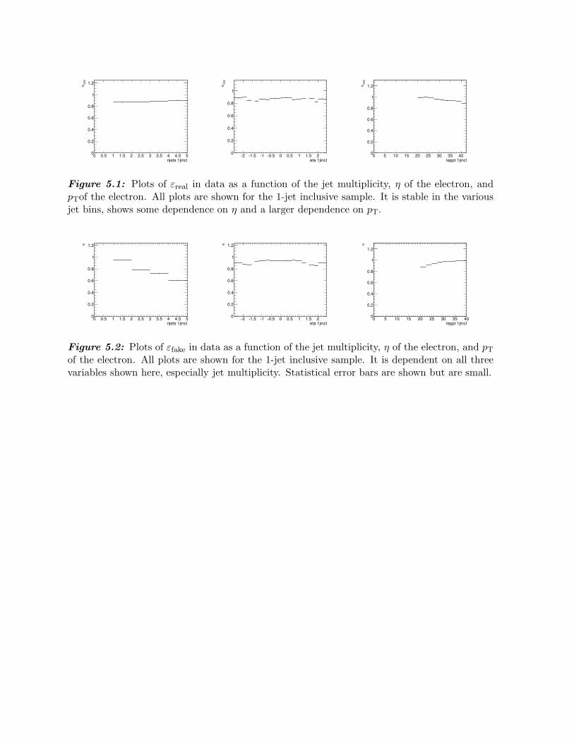
njets 1jincl0 0.5 1 1.5 2 2.5 3 3.5 4 4.5 5
rea
l∈
0
0.2
0.4
0.6
0.8
1
1.2
eta 1jincl2 1.5 1 0.5 0 0.5 1 1.5 2
rea
l∈
0
0.2
0.4
0.6
0.8
1
leppt 1jincl0 5 10 15 20 25 30 35 40
rea
l∈
0
0.2
0.4
0.6
0.8
1
1.2
Figure 5.1: Plots of εreal in data as a function of the jet multiplicity, η of the electron, andpTof the electron. All plots are shown for the 1-jet inclusive sample. It is stable in the variousjet bins, shows some dependence on η and a larger dependence on pT.
njets 1jincl0 0.5 1 1.5 2 2.5 3 3.5 4 4.5 5
∈
0
0.2
0.4
0.6
0.8
1
1.2
eta 1jincl2 1.5 1 0.5 0 0.5 1 1.5 2
∈
0
0.2
0.4
0.6
0.8
1
1.2
leppt 1jincl0 5 10 15 20 25 30 35 40
∈
0
0.2
0.4
0.6
0.8
1
1.2
Figure 5.2: Plots of εfake in data as a function of the jet multiplicity, η of the electron, and pT
of the electron. All plots are shown for the 1-jet inclusive sample. It is dependent on all threevariables shown here, especially jet multiplicity. Statistical error bars are shown but are small.


Significant. ‘So, uh, we did the green study again and got no link. It wasprobably a–’ ‘RESEARCH CONFLICTED ON GREEN JELLY BEAN/ACNE LINK;MORE STUDY RECOMMENDED!’[19]

6 The Profile Likelihood Fit
A binned profile likelihood fit to data is used to measure the parameter(s) of interest in allthree of the analyses presented in this thesis. A discriminant is chosen, and a template forthe discriminant is derived from simulation for each physical process. It is then normalized toreference values from either theoretical predictions or data, as described in Chapter 5. In thecase of the σtt-only analyses in Chapters 7 and 8, the input template is a discriminant likelihoodwhile in the three-parameter fit in Chapter 9 it is a single variable. The derivation of inputtemplates will be discussed in the appropriate chapter. A binned maximum likelihood estimatoris then used to fit the contribution of each process to the distribution observed in data. Thisserves as a measurement of the parameter(s) of interest. In this method, the expected contribu-tion of physical processes are generalized to be a function of nuisance parameters representingsystematic uncertainties. Knowledge of systematic uncertainties is then included as constraintsin the fit. In doing this, the likelihood becomes a function of both the normalization of thephysical processes and the distortions of the discriminant due to systematic uncertainties. Inthe fit, systematic uncertainties can be constrained by data to contribute less than their nominalvalue. This is achieved by using a phase space which is reduced with respect to that which anuncertainty is originally intended to cover, and by using the power of a global fit with priorknowledge regarding the normalization of physical processes and other systematic uncertaintiesincluded. The likelihood and its use are described in detail in this chapter.
6.1 The Profile Likelihood
The complete likelihood function, L, is built here. The starting point is a standard Poissonlikelihood term for each bin in the template,
Lk(µk) =µnk
k e−µk
nk!
where µk is the expected number of events in bin k and nk is the observed number of events.
Each physical process is denoted as βj, and the full set of physical processes considered
will be written as ~β. The same notation will be used for the set of all µk, written as ~µ, andsimilarly for other parameters. The expected number of events in a given bin is the cross-sectionweighted sum of all processes considered in the fit in that bin, µk(~β) =
∑
j βjνjk, where νjk
corresponds to the expected number of events from a physical process j contributing to bin k.These likelihood terms are considered to be statistically independent for each bin and thereforemultiplied together to form the basic binned likelihood for the entire template,
L0(~µ) =∏
k
Lk(µk) =∏
k
µnk
k e−µk
nk!.
The normalization of each βj is allowed to float in the fit. Any parameter of interest is uncon-strained (i.e. a flat prior is used), while background processes are constrained using a Gaussian
63

6 The Profile Likelihood Fit
prior corresponding to the uncertainty of the process’ rate, denoted ∆j. Each process is nor-malized such that βj = 1 corresponds to the nominal input cross section. The constraints areincluded as Gaussian terms in the likelihood as
C(~β) =∏
j
1√2π∆j
exp
[
− (βj − 1)2
2∆2j
]
,
where the product is over all physical processes considered. The equation for a binned templatelikelihood fit to data without the inclusion of nuisance parameters is thus built. This likelihood,Lstat = L0(~β) × C(~β), is used to determine the statistical uncertainty of the measurement.
In an extremely simple analysis with one background (unconstrained) and the signal, the fitwill find the most likely amount of contribution from each of the two processes, based on thepredicted shape of each and the data observed. In the analyses presented here, 10-20 processesare included, with background constraints as wide as ∆ ∼ 60%, depending on the channel andanalysis. The way processes are considered and their constraints change amongst the analysesand will be discussed in the appropriate chapter.
Inclusion of Systematic Uncertainties as Nuisance Parameters
The inclusion of systematic uncertainties directly into the likelihood equation gives this methodformidable power. The concept is relatively new but becoming more widely used in high energyphysics. A recent overview of the methodology is given in [124]. The expected number of eventsbecomes a function of systematic uncertainties, with each modeled as a single parameter δi.In this way, ~µ = ~µ(~β,~δ), thus L(~µ) = L(~µ(~β,~δ)). In doing this, the contribution of a givensystematic uncertainty may also be constrained within this phase space present by data whenthe global likelihood function is maximized.
Systematic uncertainties are typically given as an up and a down variation, taken to representone standard deviation (“1σ”) such that δi = 0 corresponds to the nominal case, while δi = −1is the down variation and δi = +1 is the up variation. The uncertainty is made continuous byvertical template morphing, using quadratic interpolation within δi = ±1 and linear extrapo-lation beyond, here defined up to δi = ±5 (i.e ±5σ). The morphing function for interpolationand extrapolation, ǫjik(δi), for a process j in bin k is thus defined as
ǫjik(δi) =
{ λ+jik + (δi − 1)[(3
2λ+jik − 1) + (1
2λ−jik + 1)], δi > 1
12δi[(δi − 1)λ−jik + (δi + 1)λ+
jik] − (δi − 1)(δi + 1), |δi| ≤ 1
λ−jik + (δi + 1)[(−32λ
−jik + 1) + (−1
2λ+jik − 1)], δi < −1.
Here λ+jik and λ−jik are the relative shifts in the number of expected events for a given bin and
process when taken to the positive or negative extrema of uncertainty i. The sum of expectedevents in a bin is therefore generalized to be a function of both the physical processes and thenuisance parameters, µk(~β,~δ) =
∑
j βjνjk
∏
i ǫjik(δi). The δi terms are Gaussian constrained inthe likelihood equation. The δi are normal by definition (expectation of 0, uncertainty of 1) andcan thus be written as
C(~δ) =∏
i
1√2π
exp
[
− δ2i2
]
.
where the product is over all systematic uncertainties included in the fit.
64

6.1 The Profile Likelihood
The Full Likelihood
Multiplying together the basic likelihood term with the Gaussian constraints on backgroundprocess normalizations and the nuisance parameter constraint, the full likelihood is defined as
L(~µ(~β,~δ)) = L0(~µ) × C(~β) × C(~δ)
=∏
kji
µnk
k e−µk
nk!× 1√
2π∆j
exp
[
−(βj − 1)2
2∆2j
]
× 1√2π
exp
[
−δ2i2
]
,
thereby specifying a binned likelihood including nuisance parameters for an arbitrary numberof physical processes and systematic uncertainties.
Note on Inclusion of Systematic Uncertainties in the Fit
There has been much discussion and even debate within the collaboration about what propertiesa certain systematic uncertainty must have in order to qualify for inclusion into a likelihood as anuisance parameter. The question asked for a given systematic uncertainty can be formulated as,“Can it be described by a single continuous parameter?”. One self-evident criteria is thereforethat it can be made continuous. The other is more subtle, questioning whether it can bedescribed by a single parameter. The variety of conditions and testing required means thatthe precise configuration of systematic uncertainties in the likelihood changes from analysis toanalysis in this thesis.
An example of a situation where a single parameter may not suffice is if a systematic uncer-tainty is in fact composite and would better be broken into multiple components. It should benoted that experience shows in such cases that splitting a composite uncertainty into multiplecomponents tends to yield consistent fit results with smaller uncertainties. A similar concernis that a given δi it may not be fully correlated over the full phase space used. Either casecould lead to misestimations if a single parameter is used. Through many discussions someagreements have been reached but no general rules apply. Accordingly, uncertainties are han-dled on an analysis-by-analysis basis. Much of the decision making is in fact done on the fly.Object scales and resolutions are generally considered in profiling. Some in the collaborationfeel uncomfortable profiling modeling uncertainties, resulting in them often being taken out ofthe likelihood fit for the final versions used in publications. In certain situations an uncertaintyshould a priori be included and is for the first attempt at the analysis, but pathological behavioris identified resulting in it being removed for the next iteration of fitting. This is often, butnot always, caused by a poorly thought through prescription, such as a systematic uncertaintywhich is binned in phase space and is discontinuous at certain thresholds.
In an extreme case where systematic uncertainties exhibit a degeneracy in their affect on thetemplate shape, the fit looses the power to distinguish amongst the uncertainties and gives non-sensical results. This can happen especially if several uncertainties do not affect the templateshape at all. Such “rate-only” uncertainties should be removed.
Obtaining Results from the Likelihood
Once the likelihood is defined, it can be used to estimate a parameter of interest, σtt, or multipleparameters of interest at once. For the sake of clarity the case of a single parameter of interestwill be discussed here, denoted β0. In the analyses in Chapters 7 and 8 this represents σtt andis the sole parameter of interest, while in the analysis in Chapter 9 there are three parametersof interest: σtt, fWHF
, and fWc.
65

6 The Profile Likelihood Fit
Maximizing the Likelihood
The fitter maximizes L by minimizing its negative logarithm, − ln(L), done using the MINUITpackage in ROOT [125]. Asymmetric errors are taken at the minimum using MINOS (fromMINUIT), which are used for the value quoted as the uncertainty on the parameter from the fit.Additionally, Hessian symmetric uncertainties are extracted from the second derivative at theminimum which are used only to study correlation effects. A full covariance matrix populatedwith these errors will be shown for the analyses.
Profiling the Likelihood
The profile function λ(βi) is obtained, allowing one to check the behavior of the likelihood as afunction of the parameter of interest, βi. In essence this is a projection of the likelihood functiononto a certain axis, which can be done for any parameter. To achieve this, the likelihood is firstminimized with respect to all parameters (“min”). Then a second fit (“partial”) is done whereL is minimized as a function of all parameters except for βi. The first is then subtracted fromthe second,
− ln(λ(βi)) = ln(
L(~β,~δ)min
)
− ln(
L(βi, ~β′,~δ)partial
)
,
where ~β′ in the partially minimized likelihood includes all physical processes except for βi. Intesting this is done for all parameters to identify pathological behavior in the likelihood, suchas a discontinuity or kink in the function. Plots of λ as a function of β0 will be shown in theanalyses
Marginalizing the Likelihood
An alternative method for handling nuisance parameters in a likelihood is marginalization,which integrates over the nuisance parameters. The benefit to this method is that correlationsamongst parameters can be taken into account, since the profile technique assumes uncorre-lated parameters. The downside is that it requires a numerical integration technique and istherefore computationally intensive and requires careful testing. The marginalized likelihoodis obtained by integrating
∫
L(~β,~δ)d~δ using the Metropolis-Hastings algorithm for numericalintegration [126, 127].
6.2 Evaluation of Uncertainties
The observed uncertainty at the minimum of the negative log likelihood is used to quantifythe effect of all terms minimized in the fit, namely statistical and the included systematicuncertainties. Each component’s contribution may be estimated this way. In many cases,ensemble testing is used to evaluate the behavior of the fit and estimate uncertainties. Thegeneral methodology is explained here.
Fit Uncertainty
In principle one does not access directly the observed uncertainty due to a given source inthe profile likelihood but rather observes the combined uncertainty of statistics and systematicsconsidered in the fit. The various contributions can, however, be estimated by breaking down theobserved fit uncertainty into components. The templates can be re-fit to data, removing specificsources of uncertainty from the likelihood fitting one-by-one, such that L is not a function of a
66

6.2 Evaluation of Uncertainties
specific δi, giving a result excluding that uncertainty. The relative uncertainty (since the centralvalue may shift) is calculated for each of these “N-1” tests, and subtracted in quadrature fromthe full fit result in order to estimate the contribution of the specific component in question.Doing so assumes no correlations amongst the parameters. All systematic uncertainties may beremoved, such that L = Lstat, to estimate the purely statistical component. This method onlygives approximate contributions of each uncertainty source to the fit.
Ensemble Testing
No observed data are used in ensemble testing, rather pseudo-experiments (PEs) are createdfrom the simulation. Each is intended to represent a possible outcome of the measurement.The number of events predicted in bin k as a function of the physical processes is given byµk(~β) =
∑
j βjνjk, as defined in the previous section. The actual number of events predicted fora process and bin, νjk, is calculated by using simulation for the process. To assemble a PE, νjk
is fluctuated following a certain distribution to test a specific uncertainty. Each physical sourcein a bin is fluctuated independently. The analysis is then performed, fitting the usual templatesto the PE as if it were the observed data. This process is repeated, typically thousands of times,creating an ensemble of PEs. Since the fluctuation of each PE is independent, the ensemble fitresults are expected to be Gaussian distributed around the expectation value of the fit with awidth corresponding to the magnitude of this uncertainty source in the analysis.
Statistical Uncertainty
To evaluate the expected statistical uncertainty, PEs are drawn with a Poisson fluctuation forthe expected number of events in a given bin (i.e.
√νjk). As the prediction in each bin is
essentially a multi-source counting experiment, the Poisson distribution is appropriate to use.The expected statistical uncertainty can be compared with the results of the final fit to data.The observed statistical uncertainty is a part of the fit uncertainty, and the expected statisticaluncertainty will not be used in the final results. The likelihood function Lstat is used, i.e. withno nuisance parameters.
Template Statistics Uncertainty
This method presumes that sufficient simulation statistics are available for the physical distri-bution in question to be smooth. In practice, the effect of limited simulation statistics in thetemplates can be quantified as a systematic uncertainty in the analysis. To evaluate this, PEsare constructed by first drawing from a Gaussian whose width corresponds to the simulationstatistics available, which is in turn used to draw a Poisson as described above. A Gaussian isused to reflect the assumption of large statistics. The resulting distribution is thus a convolutionof a Poisson distribution and a Gaussian distribution. In order to isolate the “template statis-tics” portion, the difference is taken in quadrature of the Poisson only test from the Gaussianand Poisson test. One can see that in the limit of infinite simulation statistics the width of theGaussian becomes negligible and the two tests return the same result, yielding no additionaluncertainty due to this limitation.
This method yields a rough estimate of the uncertainty, but in practice its magnitude gives anidea of whether or not the limited statistics are problematic in general. A large uncertainty fromthe template statistics means that the general method begins to break down. The templatesused for fitting may not be smooth enough to be reliably used. Furthermore, the PEs used fortesting can be biased if the underlying distribution does not have enough statistics.
67

6 The Profile Likelihood Fit
Systematic Uncertainty
The systematic uncertainties which are not fitted are still technically included in the definitionof the likelihood via nuisance parameters. In the fit, they are fixed to their nominal values(δi = 0). In order to evaluate the magnitude of one such “external” uncertainty in the analysis,the nuisance parameter is fixed to its extremum and PEs are drawn, fitting a Gaussian to theresults of the fit to the PEs. This fixing distorts the nominal template to be its ±1σ deviationin terms of that uncertainty. The mean of the Gaussian of fit results is taken to be the expectedfitted value, thus the uncertainty due to a given source is taken to be
< βnominal > − < βfixed delta >
< βnominal >.
To first order, the difference in the result of the fit to data with and without the parameterfixing is the magnitude of the uncertainty, but testing with PEs creates a smooth distributioninsensitive to a probable or improbable fit. The expected behavior can be evaluated using thenominal values for all parameters other than the systematic uncertainty being tested, or it canbe done using the fitted values of the likelihood to be more precise. In the results presentedhere, the fitted values are used, so the external systematic uncertainties are evaluated at theobserved minimum, not the expected. Each contribution of an external systematic is added inquadrature to the results from the fit.
Final Uncertainty
The full expected fit uncertainty, which is the observed statistical uncertainty as well as theconstrained systematic uncertainties included in the fit, can be estimated with PEs before fitting.This can be done by fluctuating ~δ and ~β within their uncertainty as well as allowing the Poissonfluctuation on statistical uncertainty. As for the pure statistical test, this checks the fit behaviorbut will not be used in final results.
The final quoted uncertainty on a measurement is the sum in quadrature of the fit uncertainty(which includes observed statistical uncertainty) and all externally evaluated systematic uncer-tainties (including template statistics). Following convention, the uncertainty will be quotedboth in total and broken down into components as statistical, systematic, and luminosity. Thefit uncertainty is broken down into its components as statistical and systematic uncertaintiesusing the statistics-only fit and N-1 testing.
Linearity Tests
The linearity of the fit is checked using ensemble testing in order to further ensure a non-biasedresult. The parameter of interest is set to a given value other than 1 before a PE is drawn. PEsare then drawn at each of many points across a large range, and the central values with theirRMS are then plotted. A line is fit through the points. A perfectly unbiased fit should returna slope of 1 with a y-intercept of 0. For testing σtt, input values are injected for over the range[120, 200] pb in steps of 20 pb in all three analyses. For the 3-parameter analysis in Chapter 9,linearity each of the flavor ratios is checked for over a range of [0.4, 2.0] in steps of 0.2. If asignificant bias is found, the results of the fit can be corrected for a posteriori.
68


Turn-On. “Supercollider? I ‘ardly know ‘er!”[19]

7 Measurement of σtt in∫
L dt = 35 pb−1
Using b-tagging
The single most precise measurement of σtt at ATLAS using the∫
L dt= 35 pb−1 dataset col-lected during 2010 has been submitted for publication to Physics Letters B [17] and is shownhere. The measurement uses the semileptonic decay channel of tt in both the e+jets and µ+jetschannels. A binned profile likelihood template fit to data is used to extract the signal, withmany systematic uncertainties included in the fit as nuisance parameters. The templates usedin the fit are a discriminant likelihood constructed from kinematic variables and a flavor sensitiveb-tagging weight variable, which is optimized to discriminate the tt process from W+jets.
7.1 Selection
The events selected in this analysis have a high pT, prompt lepton (e,µ), multiple jets, and largemissing energy, summarized in Section 4.3. The event yields are shown in Table 7.1 for µ+jets(upper) and e+jets (lower) channels in each jet bin. In the fit, events with three or more jetsare used with each lepton for a total of 6 channels. The 1-2 jet bins are shown as a controlregion. The fake lepton contribution is taken from the anti-electron fitting method for e+jetsand the matrix method for µ+jets, as discussed in Section 5.2. Basic kinematic plots in both thelow jet multiplicity control region and high jet multiplicity signal region are shown for e+jets inAppendix C.
7.2 The Input Distribution
The discriminant is a likelihood which takes four variables as input, and is trained to discriminatett from W+jets based on MC simulation. The training of the likelihood discriminant and itsevaluation is done using TMVA [128], which trains for signal divided by signal over background,S/S+B. The shape of W+jets is taken as representative of all of the background processes forthe training process. It is expected to be the dominant source of background events, as canbe seen in Table 7.1. For tt and W+jets the MC is split in half, where one half is used as areference sample to train the likelihood and the other half is used in evaluation, that is, to createthe template for the process to be used in the fit. The discriminant is evaluated for all otherbackground processes and data as well.
The W+jets sample includes all of the various flavor contributions, scaled as discussed inSection 5.1. The analysis is flavor-sensitive due to the inclusion of continuous b-tagging as aninput to the discriminant likelihood. The variables which are used as input are described here,and the discriminant is shown before the fit.
Lepton Pseudorapidity
Lepton pseudorapidity (η) is a simple physical quantity which is quite useful in discriminatingtt from W+jets, due to the differing production mechanisms of the leptonically decaying W . In
71
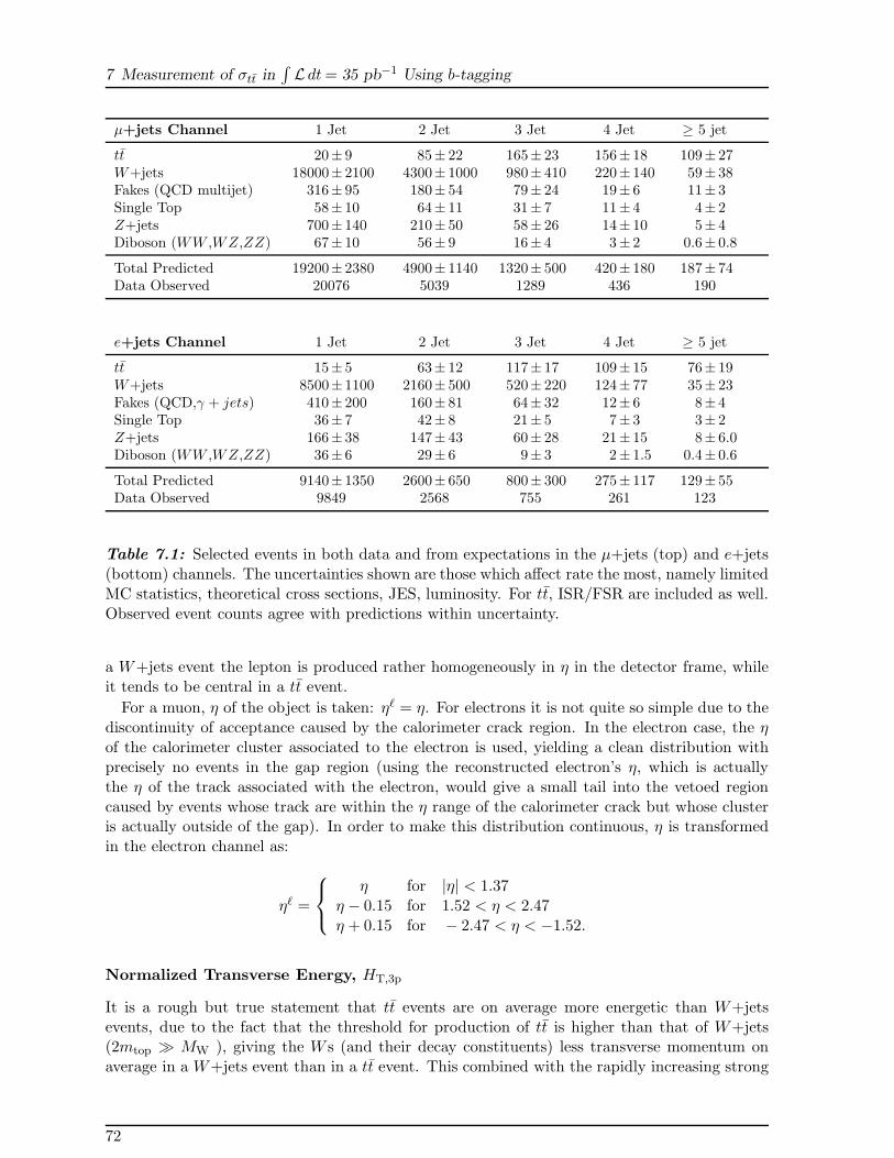
7 Measurement of σtt in∫
L dt= 35 pb−1 Using b-tagging
µ+jets Channel 1 Jet 2 Jet 3 Jet 4 Jet ≥ 5 jet
tt 20± 9 85± 22 165± 23 156± 18 109± 27W+jets 18000± 2100 4300± 1000 980± 410 220± 140 59± 38Fakes (QCD multijet) 316± 95 180± 54 79± 24 19± 6 11± 3Single Top 58± 10 64± 11 31± 7 11± 4 4± 2Z+jets 700± 140 210± 50 58± 26 14± 10 5± 4Diboson (WW ,WZ,ZZ) 67± 10 56± 9 16± 4 3± 2 0.6± 0.8
Total Predicted 19200± 2380 4900± 1140 1320± 500 420± 180 187± 74Data Observed 20076 5039 1289 436 190
e+jets Channel 1 Jet 2 Jet 3 Jet 4 Jet ≥ 5 jet
tt 15± 5 63± 12 117± 17 109± 15 76± 19W+jets 8500± 1100 2160± 500 520± 220 124± 77 35± 23Fakes (QCD,γ + jets) 410± 200 160± 81 64± 32 12± 6 8± 4Single Top 36± 7 42± 8 21± 5 7± 3 3± 2Z+jets 166± 38 147± 43 60± 28 21± 15 8± 6.0Diboson (WW ,WZ,ZZ) 36± 6 29± 6 9± 3 2± 1.5 0.4± 0.6
Total Predicted 9140± 1350 2600± 650 800± 300 275± 117 129± 55Data Observed 9849 2568 755 261 123
Table 7.1: Selected events in both data and from expectations in the µ+jets (top) and e+jets(bottom) channels. The uncertainties shown are those which affect rate the most, namely limitedMC statistics, theoretical cross sections, JES, luminosity. For tt, ISR/FSR are included as well.Observed event counts agree with predictions within uncertainty.
a W+jets event the lepton is produced rather homogeneously in η in the detector frame, whileit tends to be central in a tt event.
For a muon, η of the object is taken: ηℓ = η. For electrons it is not quite so simple due to thediscontinuity of acceptance caused by the calorimeter crack region. In the electron case, the ηof the calorimeter cluster associated to the electron is used, yielding a clean distribution withprecisely no events in the gap region (using the reconstructed electron’s η, which is actuallythe η of the track associated with the electron, would give a small tail into the vetoed regioncaused by events whose track are within the η range of the calorimeter crack but whose clusteris actually outside of the gap). In order to make this distribution continuous, η is transformedin the electron channel as:
ηℓ =
η for |η| < 1.37η − 0.15 for 1.52 < η < 2.47η + 0.15 for − 2.47 < η < −1.52.
Normalized Transverse Energy, HT,3p
It is a rough but true statement that tt events are on average more energetic than W+jetsevents, due to the fact that the threshold for production of tt is higher than that of W+jets(2mtop ≫ MW ), giving the W s (and their decay constituents) less transverse momentum onaverage in a W+jets event than in a tt event. This combined with the rapidly increasing strong
72

7.2 The Input Distribution
coupling strength at low energies means that the additional jets due to QCD jet production inassociation with the W will tend to be soft, indeed far softer on average than the jets in a ttevent.
One can construct a class of variables known as HT which are a measure the transversemomentum of the event as a whole. It has been found by testing that the transverse momentumof third and fourth jets yield a particularly high separation power; their sum therefore formsthe numerator of the variable used. In the 3-jet bin it is only the third jet, and in the lower jetbins the variable is not defined. Higher jets were left out in order to control pileup and largeradiation effects, because the 5-jet bin is inclusive and could have many more jets present. Thedenominator is the sum of the absolute value of the longitudinal momentum, pz, of all objectsin the event, including the neutrino, which is calculated using the event kinematics and solvedfor by taking the smaller neutrino solution. This variable, called HT,3p, is defined as:
HT,3p =
∑Njets≤4i=3 |p2
T,i|∑Nobjects
j=1 |pz,j|.
This definition as such yields a particularly clumped distribution, so it is transformed asHT,3p → exp(−4 ×HT,3p) to obtain a smoother input distribution for the likelihood discrimi-nant.
Aplanarity
The aplanarity A is a measure of the topography of the event. A is defined as 1.5 times thesmallest eigenvalue of the momentum tensor, which is defined as:
Mij =
∑Nobjects
k=1 pikpjk∑Nobjects
k=1 p2k
,
where pik is the i-th momentum component of object k and pk is the absolute value of itsmomentum. All jets in the event and the charged lepton are considered in the definition. Theresult is a clumped distribution which is smoothed by transforming A→ exp(−8 ×A).
Mean of Two Highest JetProb Weights
The output of the JetProb algorithm, discussed in Section 4.4, is used as an input to thelikelihood. Based on the knowledge that a tt event should contain two b-jets, a variable isconstructed which is the mean of the b-tagging algorithm’s value for two most b-like jets. Thisvariable, wJP, shows a strong discriminating power due to the fact that W+jets events aredominated by light jet production. Nonetheless, the uncertainty on fWHF
is large enough thatthis becomes a sizable uncertainty in the analysis. Furthermore the uncertainty in the calibrationof the algorithm, a process described in Section 4.4, becomes a large systematic uncertainty.
After the calibration procedure described in Section 4.4 was applied, a remnant discrepancy inthe background dominated events in the light part of the spectrum – below the lowest calibratedworking point – was observed. While unfortunate this is not particularly surprising, as thealgorithm is only very roughly calibrated in this regime. This is handled in two ways in theanalysis. In the distribution, all points below the lowest working point are lumped together intoa single bin, averaging out the coarse calibration. The problem is solved in the bins which havea high signal to background ratio (4 and 5 jets). In the background dominated 3-jet bin it isthought that the mismodeling is too dramatic to be trustworthy. Accordingly the variable wJP
is not used in the 3-jet bin but is still used in the others.
73

7 Measurement of σtt in∫
L dt= 35 pb−1 Using b-tagging
The Input Likelihood
The four variables (three in the 3-jet bin, without wJP) are combined into a likelihood discrim-inant for each of the six physics channels: e+jets and µ+jets, which are further split into 3-jetexclusive, 4-jet exclusive, and 5-jet inclusive events. These six physics channels are treated onequal footing in the fit, with 20 bins in each histogram, yielding a total 120-bin fit. In addition tobeing necessary following the theoretical considerations in the introduction, for similar reasonsthis serves to mitigate systematic uncertainties by absorbing signal events which migrate awayfrom the 4-jet bin. Furthermore, the 3-jet bins serve to constrain the background contribution.
The expected separation between W+jets and tt can be seen in each channel in Figure 7.1.One can see that the 3-jet bin in both channels suffers from a significantly lower discriminatingpower due to omitting wJP in the likelihood discriminant. A clean separation between signaland background is achieved in particular in the 4-jet bins and the µ+5 jet bin. This is notthe case in e+5 jets due to the significantly reduced background fraction in the channel, whichcomes from the harsher cuts to control the fake rate, reducing an already small background inthe 5-jet bin to be even smaller in the electron channel. The sum of all prediction contributionsis compared to the data before the fit in Figure 7.2.
Validation
The variables have been chosen based on expected discriminant power, with potential sensitivityto systematic uncertainties taken into account in the decision as well. It is essential to validate thechoices to ensure that the variables are well-modeled, in particular in the background dominatedregions. The set of variables used in the analysis is shown both in the two-jet control regionand in the signal region for both channels. There is generally a good agreement between MCpredictions and measured data. The data-MC agreement is shown for the variables of interest inFigures 7.7-7.14 at the end of this chapter. No discrepancies beyond uncertainties are observed.
7.3 The Fit Likelihood
The profile likelihood formalism developed in Chapter 6 is used to fit the discriminant templatesfor the signal and various backgrounds to data. The choices made are described here, and theexpected behavior of the fit is evaluated as necessary.
The Fit Parameters
The sole parameter of interest in this six-channel, 120 bin fit is σtt. Prior knowledge of the variousbackgrounds are included in the fit as constraints, and nuisance parameters describing systematicuncertainties are included and potentially constrained. The main background, W+jets, is takenas uncorrelated a priori amongst the six channels, with the uncertainty on the normalizationin each jet bin increasing from bin to bin. The uncertainty on fWHF
and fWc are handledin terms of nuisance parameters, with one for fWHF
and another for fWc in each of the jetbins, taken as correlated between the two lepton channels, for a total of 6 δs. The QCDmultijet production is treated a priori uncorrelated in each jet bin and channel as well, witha flat 50 % normalization uncertainty for each. The uncertainty due to the shape of QCDmultijet production is not treated as a nuisance parameter due to its discrete nature. Thenormalization of smaller electroweak background (Z+jets, single top, and di-boson production)are each treated as a single β parameter in the fit, each constrained within their theoreticaluncertainty. No modeling uncertainty is considered for these processes. The small magnitude of
74

7.3 The Fit Likelihood
Likelihood Discriminant0 20 40 60 80 100
Arb
itra
ry U
nit
s
0
0.01
0.02
0.03
0.04
0.05
0.06
0.07
Figure 7.1: The separation power of the likelihood discriminant in all six analysis bins, com-paring tt (red) and W+jets (black). The left three plots are µ+jets, the right three are e+jets.In each channel, from left to right each group of twenty bins are 3-jet exclusive, 4-jet exclusive,and 5-jet inclusive.
these backgrounds in the signal region and the relative insensitivity of the fit to them warrantssuch treatment. The βs and their constraints are summarized in Table 7.2.
The dominant object-related uncertainties are the b-tag and mistag scale factors at each of thefour calibrated operating points, which are each profiled as independent nuisance parameters,totaling 8 in all. All object related uncertainties (energy scales, efficiencies, and resolutions)are profiled in the likelihood as well. The uncertainty due to PDFs are not included in thefit because there are too many uncorrelated parameters; including them would have effectivelydoubled the number of degrees of freedom in the fit, which is simply impractical. After muchdiscussion, uncertainties which are not clearly continuous – the signal generator, the partonshower, W+jets shape, and the QCD model – are not included in the fit. In such cases theinterpretation of the result of the nuisance parameter in the fit are too unclear for the taste ofsome. In a similar fashion, much work was done by others to show that initial and final stateradiation (ISR/FSR) could be considered as a continuous uncertainty and thus cleanly includedin the fit. This came under heavy fire during collaboration review and they have thus beenremoved from the fit, meanwhile scientific publications have ascended to the status of laws andsausages, being things which one is better off not seeing being made.
75
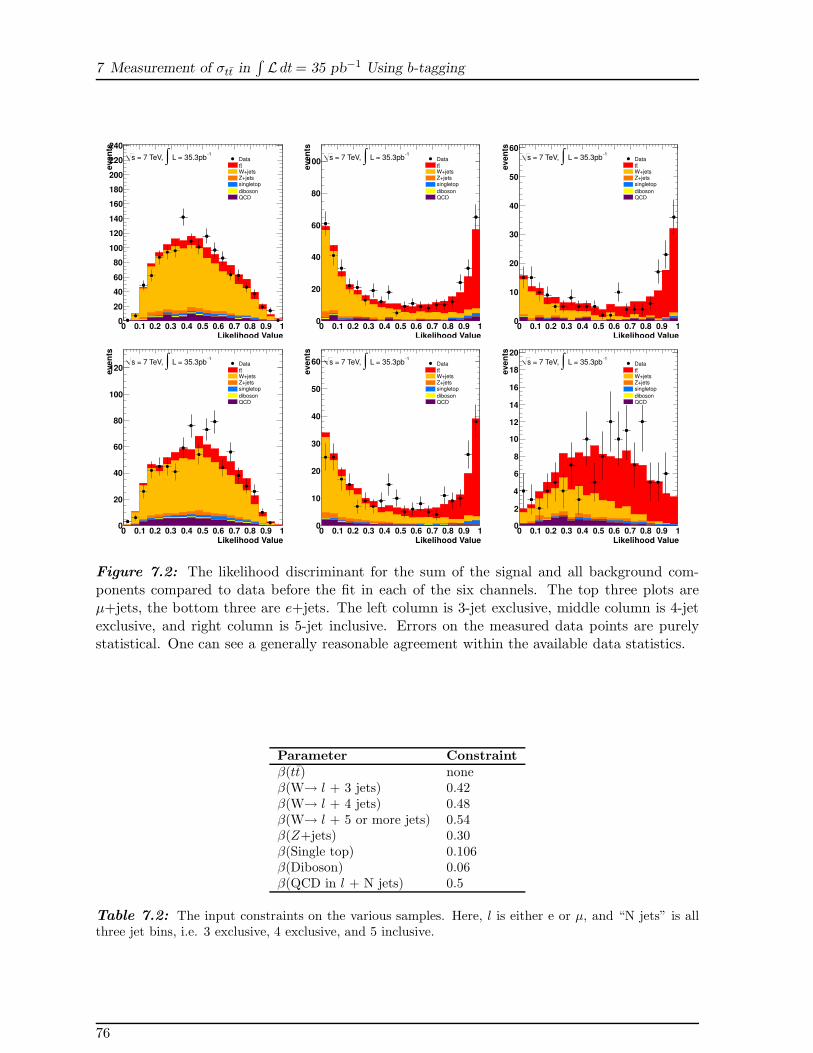
7 Measurement of σtt in∫
L dt= 35 pb−1 Using b-tagging
Likelihood Value0 0.1 0.2 0.3 0.4 0.5 0.6 0.7 0.8 0.9 1
even
ts
0
20
40
60
80
100
120
140
160
180
200
220
240
Data
ttW+jetsZ+jetssingletop
dibosonQCD
1 L = 35.3pb∫ = 7 TeV, s
Likelihood Value0 0.1 0.2 0.3 0.4 0.5 0.6 0.7 0.8 0.9 1
even
ts
0
20
40
60
80
100 Data
ttW+jetsZ+jetssingletop
dibosonQCD
1 L = 35.3pb∫ = 7 TeV, s
Likelihood Value0 0.1 0.2 0.3 0.4 0.5 0.6 0.7 0.8 0.9 1
even
ts
0
10
20
30
40
50
60
Data
ttW+jetsZ+jetssingletop
dibosonQCD
1 L = 35.3pb∫ = 7 TeV, s
Likelihood Value0 0.1 0.2 0.3 0.4 0.5 0.6 0.7 0.8 0.9 1
even
ts
0
20
40
60
80
100
120Data
ttW+jetsZ+jetssingletop
dibosonQCD
1 L = 35.3pb∫ = 7 TeV, s
Likelihood Value0 0.1 0.2 0.3 0.4 0.5 0.6 0.7 0.8 0.9 1
even
ts
0
10
20
30
40
50
60 Data
ttW+jetsZ+jetssingletop
dibosonQCD
1 L = 35.3pb∫ = 7 TeV, s
Likelihood Value0 0.1 0.2 0.3 0.4 0.5 0.6 0.7 0.8 0.9 1
even
ts
0
2
4
6
8
10
12
14
16
18
20
Data
ttW+jetsZ+jetssingletop
dibosonQCD
1 L = 35.3pb∫ = 7 TeV, s
Figure 7.2: The likelihood discriminant for the sum of the signal and all background com-ponents compared to data before the fit in each of the six channels. The top three plots areµ+jets, the bottom three are e+jets. The left column is 3-jet exclusive, middle column is 4-jetexclusive, and right column is 5-jet inclusive. Errors on the measured data points are purelystatistical. One can see a generally reasonable agreement within the available data statistics.
Parameter Constraintβ(tt) noneβ(W→ l + 3 jets) 0.42β(W→ l + 4 jets) 0.48β(W→ l + 5 or more jets) 0.54β(Z+jets) 0.30β(Single top) 0.106β(Diboson) 0.06β(QCD in l + N jets) 0.5
Table 7.2: The input constraints on the various samples. Here, l is either e or µ, and “N jets” is allthree jet bins, i.e. 3 exclusive, 4 exclusive, and 5 inclusive.
76

7.4 Results of the Fit and Systematic Uncertainties
Behavior of the Fit
The linearity of the fit is checked in steps of 10 pb over the range [120,200] pb, with results shownin Figure 7.3. A small offset of -1.6 pb is identified and corrected for in the final fit.
[pb]tt
σInput 120 140 160 180 200
[pb]
ttσ
Fitte
d
120
140
160
180
200
/ ndf 2χ 5.020 / 7
p0 1.210± 1.644
p1 0.008± 0.994
/ ndf 2χ 5.020 / 7
p0 1.210± 1.644
p1 0.008± 0.994
Figure 7.3: The linearity of the fit over the range σtt = [120,200] pb. A small offset of about1.6 pb is observed (the y-intercept, p0, of the fit), for which the final results are corrected.
7.4 Results of the Fit and Systematic Uncertainties
After correcting for the small offset observed in the linearity test, the result of the fit is
σtt = 187+16−15 (fit) pb.
The externally evaluated systematic uncertainties are not yet added to the uncertainty. Thefitted result is shown in Figure 7.4, where excellent data-MC agreement can be seen. The fullcorrelation matrix of all ~β and ~δ are shown in Figure 7.5. All observed correlations are asexpected and not particularly strong. The profiled likelihood as a function of σtt is shown nearthe minimum in Figure 7.6. A smooth curve is observed. The results of the fit for every βand δ parameter can be seen in Table 7.3, all of which are consistent with expectations withinuncertainty.
The systematic uncertainties considered in this analysis are summarized and discussed through-out Chapters 3–5 and listed in Appendix A. The magnitude of the uncertainties in this analysisare summarized in Table 7.4, evaluated following the procedure developed in Chapter 6. One cansee that the analysis is clearly dominated by systematic uncertainty, although statistical uncer-tainty is the single largest contribution, at about 6% relative uncertainty on σtt. The dominantsystematic uncertainties are the b-tagging algorithm calibration and ISR/FSR modeling for tt,each contributing about 5 %. The sub-leading uncertainties at 3-4 % are MC generator choice,jet energy scale, and the uncertainty on fWHF
.
77
7 Measurement of σtt in∫
L dt= 35 pb−1 Using b-tagging
Once including all external systematic uncertainties, the final result of this analysis is
σtt = 187 ± 11(stat.) +18−17(syst.) ± 6(lumi.) pb = 187+22
−21 pb.
This represents the single most precise measurement of σtt with the 2010∫
L dt= 35 pb−1
dataset at ATLAS. Interpretation of this result will be discussed in Chapter 10.
Cross Checks
A number of checks of the fit have been done, in particular testing stability of the central valueand assumptions made in the nuisance parameters. Concern was raised during collaborationreview of this work surrounding the legitimacy of including each JES term as a single nuisanceparameter, since this presumes a correlation across phase space. Studies indicated that corre-lations were at the 90% level, implying a negligible effect of the assumption of full correlation.Extensive testing was nonetheless undertaken.
An example of a test performed was to first re-fit after removing a nuisance parameter fromthe likelihood (the calorimeter JES component) and comparing results with the nominal, asa check of stability and uncertainty estimation. Results were found to be stable within theuncertainty caused by that additional term. A further test was to assume different correlationsin pT and η, to check if uncertainty was being underestimated by using one part of phase space toconstrain another where no such correlation should be assumed. To do this, the uncertainty wassplit into three components: 50 % of the uncertainty was treated normally, while 25 % increasedwith jet pT and 25 % decreased. The test was constructed such that for any jet pT, the sumof the three terms would yield the default uncertainty. The overall fit uncertainty was foundto be lower than in the nominal case. In another case, the component’s magnitude was variedup and down additionally as a function of jet |η|, and the resulting uncertainty was found tobe compatible. These tests, and several others documented fully in Appendix C of [14], showedstable, consistent results with well estimated uncertainties.
78

7.4 Results of the Fit and Systematic Uncertainties
Likelihood Discriminant
0 20 40 60 80 100
En
trie
s
0
20
40
60
80
100
120
140
160
KS test:0.901
test:0.3082χ = 7 TeVs, 1
L dt = 35.3 pb∫
0 20 40 60 80 100
Ra
tio
Da
ta/F
it
0
0.5
1
1.5
2
Figure 7.4: The fitted result compared with the data, showing excellent agreement overall.The left three channels are µ+jets, the right three are e+jets. Both count 3-jet exclusive, 4-jetexclusive, and 5-jet inclusive. Each of the six channels has 20 bins in the fit.
79

7 Measurement of σtt in∫
L dt= 35 pb−1 Using b-tagging
1
0.5
0
0.5
1
)t(tβ
+ 3
je
ts)
µ→
(Wβ +
4 je
ts)
µ→
(Wβ +
5 je
ts)
µ→
(Wβ e
+ 3
je
ts)
→(Wβ
e +
4 je
ts)
→(Wβ
e +
5 je
ts)
→(Wβ
(Z+
Je
ts)
β(S
ing
le t
op
)β
(Dib
oso
n)
β +
3 je
ts)
µ(Q
CD
in
β
+ 4
je
ts)
µ(Q
CD
in
β
+ 5
je
ts)
µ(Q
CD
in
β
(QC
D in
e +
3 je
ts)
β (QC
D in
e +
4 je
ts)
β (QC
D in
e +
5 je
ts)
β(b
ta
gg
ing
WP
1)
δ (bt
ag
gin
g W
P2
)δ (b
ta
gg
ing
WP
3)
δ (bt
ag
gin
g W
P4
)δ
(mis
tag
s W
P1
)δ (m
ista
gs W
P2
)δ (m
ista
gs W
P3
)δ (m
ista
gs W
P4
)δ (J
et
Eff
icie
ncy)
δ(J
ER
)δ
3je
t)c
/cb
(W+
bδ
4je
t)c
/cb
(W+
bδ
5je
t)c
/cb
(W+
bδ
(W+
c 3
jet)
δ (W+
c 4
jet)
δ (W+
c 5
jet)
δ(P
ileu
p)
δ S
Fs)
µ(δ(e
SF
s)
δ M
om
en
tum
Sm
ea
rin
g)
µ(δ(e
Re
so
lutio
n S
me
arin
g)
δ(e
En
erg
y S
ca
le)
δ)
T(M
issin
g E
δ(E
taJE
S)
δ (Ca
loJE
S)
δ(A
lpg
en
JE
S)
δ(N
ois
eJE
S)
δ (Pile
up
JE
S)
δ (Pe
rug
iaJE
S)
δ(b
JE
S)
δ(J
ES
fla
vo
ur)
δ (JE
S c
lose
by)
δ)t(tβ
+ 3 jets)µ→(Wβ + 4 jets)µ→(Wβ + 5 jets)µ→(Wβ
e + 3 jets)→(Wβ e + 4 jets)→(Wβ e + 5 jets)→(Wβ
(Z+Jets)β(Single top)β
(Diboson)β + 3 jets)µ(QCD in β + 4 jets)µ(QCD in β + 5 jets)µ(QCD in β
(QCD in e + 3 jets)β(QCD in e + 4 jets)β(QCD in e + 5 jets)β
(btagging WP1)δ(btagging WP2)δ(btagging WP3)δ(btagging WP4)δ
(mistags WP1)δ(mistags WP2)δ(mistags WP3)δ(mistags WP4)δ(Jet Efficiency)δ
(JER)δ 3jet)c/cb(W+bδ 4jet)c/cb(W+bδ 5jet)c/cb(W+bδ
(W+c 3jet)δ(W+c 4jet)δ(W+c 5jet)δ
(Pileup)δ SFs)µ(δ
(e SFs)δ Momentum Smearing)µ(δ
(e Resolution Smearing)δ(e Energy Scale)δ
)T
(Missing Eδ (EtaJES)δ(CaloJES)δ
(AlpgenJES)δ(NoiseJES)δ(PileupJES)δ
(PerugiaJES)δ(bJES)δ
(JES flavour)δ(JES closeby)δ
Figure 7.5: The correlation amongst all parameters in the fit, obtained from the fit to data.Correlations are as expected.
80

7.4 Results of the Fit and Systematic Uncertainties
0β
0 0.2 0.4 0.6 0.8 1 1.2 1.4 1.6 1.8 2 2.2
)0β(λ
ln
0
2
4
6
8
10
12
14
16
18
20
Figure 7.6: The profile likelihood as a function of σtt is shown near its minimum. Smoothprofiling is observed.
81

7 Measurement of σtt in∫
L dt= 35 pb−1 Using b-tagging
Parameter Value Error Error Up Error Down
β(tt) 1.1236 0.0944 0.1011 -0.0906β(W in µ + 3 jets) 0.8771 0.0873 0.1061 -0.0809β(W in µ + 4 jets) 0.8575 0.1279 0.1527 -0.1178β(W in µ + 5 jets) 0.7588 0.2163 0.2578 -0.1957β(W in e + 3 jets) 0.9124 0.1025 0.1060 -0.0994β(W in e + 4 jets) 0.8479 0.1547 0.1607 -0.1490β(W in e + 5 jets) 0.5844 0.2592 0.2741 -0.2455β(Z+Jets) 1.1180 0.2796 0.2791 -0.2828β(Single top) 1.0056 0.1059 0.1059 -0.1059β(Diboson) 1.0007 0.0600 0.0600 -0.0600β(QCD in µ + 3 jets) 0.9094 0.4785 0.4803 -0.4801β(QCD in µ + 4 jets) 1.0096 0.4729 0.4732 -0.4733β(QCD in µ + 5 jets) 0.6455 0.4722 0.4729 -0.4723β(QCD in e + 3 jets) 1.0655 0.4881 0.4906 -0.4910β(QCD in e + 4 jets) 1.0080 0.4966 0.4971 -0.4972β(QCD in e + 5 jets) 0.8557 0.4909 0.4916 -0.4915
δ(b-tag WP1) -0.7265 1.0978 1.1107 -0.9672δ(b-tag WP2) 0.6253 0.9646 0.9566 -0.9658δ(b-tag WP3) -0.0318 0.9121 0.9080 -0.9163δ(b-tag WP4) 0.2144 0.8694 0.8813 -0.8627δ(mistag WP1) 0.3433 1.0025 0.9824 -1.0130δ(mistag WP2) -0.3573 0.9745 0.9741 -0.9727δ(mistag WP3) 0.3048 0.9900 0.9863 -0.9889δ(mistag WP4) 0.0155 0.9951 0.9952 -0.9950δ(JES) 0.9877 0.5286 0.5418 -0.5090δ(JER) 0.5819 0.9077 0.9060 -0.9213δ(W+bb/cc Fraction 3 jets) -0.5879 0.9566 0.9557 -0.9602δ(W+bb/cc Fraction 4 jets) 0.1945 0.8674 0.8772 -0.8620δ(W+bb/cc Fraction 5 jets) -0.3314 0.9168 0.9423 -0.8981δ(W+c Fraction 3 jets) 0.4251 0.9473 0.9467 -0.9480δ(W+c Fraction 4 jets) 0.0570 0.9766 0.9764 -0.9768δ(W+c Fraction 5 jets) -0.1269 0.9974 0.9974 -0.9974δ(Pileup) 0.2372 0.7695 0.7623 -0.7758δ(µ SFs) -0.0480 0.9875 0.9875 -0.9870δ(e SFs) 0.0570 0.9400 0.9413 -0.9371δ(µ Momentum Smearing) -0.1645 1.3664 1.1531 -1.3183δ(e Energy Resolution) 0.1638 0.7652 0.7534 -0.7627δ(e Energy Smearing) 0.2623 0.7817 0.7526 -0.7935δ(Missing Et) -0.3195 0.6002 0.6361 -0.5551δ(JES Eta) 1.0882 0.4783 0.4909 -0.5229δ(JES Calo) -0.6341 0.4880 0.5793 -0.4338δ(JES Alpgen) -0.6025 0.5713 0.7319 -0.4873δ(JES Noise) -0.2967 0.7438 0.8626 -0.6115δ(JES Pileup) 0.0959 0.6814 0.6229 -0.6804δ(JES Perugia) -0.0567 0.3534 0.2697 -0.9915δ(JES b-Jet) -0.3575 0.7138 0.7607 -0.6514
Table 7.3: The full results of the fit for ~β and ~δ including their uncertainties. The asymmetricerror is observed at the fit minimum and the symmetric errors are from the hessian error matrix.
82

7.4 Results of the Fit and Systematic Uncertainties
Statistical Uncertainty (%) +5.8 -5.7
Simulation (%)
b-tagging calibration +4.1 -3.8Jet energy scale +3.9 -2.9Jet reconstruction efficiency +0.01 -0.3Jet energy resolution +0.3 -0.01Electron scale factor +1.6 -1.4Muon scale factor +1.2 -1.1Electron smearing +0.0 -0.0Muon smearing +0.4 -0.4Electron energy scale +0.5 -0.3Emiss
T (softjet + cellout) +0.01 -0.01Emiss
T (pileup) +0.01 -0.01
Background Modeling (%)
W+jets HF content +2.7 -2.4W+jets shape +1.0 -1.0QCD shape +0.8 -0.8
tt Signal Modeling (%)
ISR/FSR +5.2 -5.2MC Generator +4.2 -4.2Hadronization +0.4 -0.4PDF +1.5 -1.5
Method (%)
Templates statistics +1.1 -1.1
Total Systematic (%) +9.7 -9.0
Table 7.4: Table of estimated systematic uncertainties. Systematic uncertainties includedin the fit are estimated by N-1 testing. The remaining systematic uncertainties are added inquadrature afterwards. Statistical uncertainty is the single largest component but systematicuncertainty dominates overall.
83

7 Measurement of σtt in∫
L dt= 35 pb−1 Using b-tagging
)µ(η2.5 2 1.5 1 0.5 0 0.5 1 1.5 2 2.5
En
trie
s/0
.50
0
200
400
600
800
1000data
ttW+JetsQCDOther
1 L dt = 35 pb∫
+ 2 Jetsµ
)µ(η2.5 2 1.5 1 0.5 0 0.5 1 1.5 2 2.5
En
trie
s/0
.50
0
50
100
150
200
250
300
data
ttW+JetsQCDOther
1 L dt = 35 pb∫
+ 3 Jetsµ
)µ(η2.5 2 1.5 1 0.5 0 0.5 1 1.5 2 2.5
En
trie
s/0
.50
0
20
40
60
80
100 data
ttW+JetsQCDOther
1 L dt = 35 pb∫
+ 4 Jetsµ
)µ(η2.5 2 1.5 1 0.5 0 0.5 1 1.5 2 2.5
En
trie
s/0
.50
0
10
20
30
40
50 data
ttW+JetsQCDOther
1 L dt = 35 pb∫
5 Jets≥ + µ
Figure 7.7: The input variable ηℓ for the likelihood discriminant in the µ+jets channel. The2-jet bin is shown as a control region (top left), and the signal region is shown in the 3-jet bin(top center), 4-jet bin (top right) and 5-jet inclusive bin (lower left).
Aplanarity)×exp(8
0 0.1 0.2 0.3 0.4 0.5 0.6 0.7 0.8 0.9 1
En
trie
s/0
.10
0
500
1000
1500
2000
2500
3000
3500
4000
4500data
ttW+JetsQCDOther
1 L dt = 35 pb∫
+ 2 Jetsµ
Aplanarity)×exp(8
0 0.1 0.2 0.3 0.4 0.5 0.6 0.7 0.8 0.9 1
En
trie
s/0
.10
0
100
200
300
400
500
600
700
data
ttW+JetsQCDOther
1 L dt = 35 pb∫
+ 3 Jetsµ
Aplanarity)×exp(8
0 0.1 0.2 0.3 0.4 0.5 0.6 0.7 0.8 0.9 1
En
trie
s/0
.10
0
20
40
60
80
100
120
140
160data
ttW+JetsQCDOther
1 L dt = 35 pb∫
+ 4 Jetsµ
Aplanarity)×exp(8
0 0.1 0.2 0.3 0.4 0.5 0.6 0.7 0.8 0.9 1
En
trie
s/0
.10
0
10
20
30
40
50
60data
ttW+JetsQCDOther
1 L dt = 35 pb∫
5 Jets≥ + µ
Figure 7.8: The input variable exp(−8 ×A) for the likelihood discriminant in the µ+jetschannel. The 2-jet bin is shown as a control region (top left), and the signal region is shown inthe 3-jet bin (top center), 4-jet bin (top right) and 5-jet inclusive bin (lower left).
84

)T,3pH×exp(4
0 0.2 0.4 0.6 0.8 1
En
trie
s/0
.10
0
100
200
300
400
500
600
700 data
ttW+JetsQCDOther
1 L dt = 35 pb∫
+ 3 Jetsµ
)T,3pH×exp(4
0 0.2 0.4 0.6 0.8 1
En
trie
s/0
.10
0
20
40
60
80
100
120
140
160
180
data
ttW+JetsQCDOther
1 L dt = 35 pb∫
+ 4 Jetsµ
)T,3pH×exp(4
0 0.2 0.4 0.6 0.8 1
En
trie
s/0
.10
0
10
20
30
40
50
60
70data
ttW+JetsQCDOther
1 L dt = 35 pb∫
5 Jets≥ + µ
Figure 7.9: The input variable exp(−4 ×HT,3p) for the likelihood discriminant in the µ+jetschannel. By definition the variable can only be constructed in events with 3 or more jets. Thesignal region is shown in the 3-jet bin (left), 4-jet bin (center) and 5-jet inclusive bin (right).
JPw
0 2 4 6 8 10 12 14
En
trie
s/0
.50
0
500
1000
1500
2000
2500
3000data
ttW+JetsQCDOther
1 L dt = 35 pb∫
+ 2 Jetsµ
JPw
0 2 4 6 8 10 12 14
En
trie
s/0
.50
0
100
200
300
400
500
600data
ttW+JetsQCDOther
1 L dt = 35 pb∫
+ 3 Jetsµ
JPw
0 2 4 6 8 10 12 14
En
trie
s/0
.50
0
20
40
60
80
100
120 data
ttW+JetsQCDOther
1 L dt = 35 pb∫
+ 4 Jetsµ
JPw
0 2 4 6 8 10 12 14
En
trie
s/0
.50
0
10
20
30
40
50 data
ttW+JetsQCDOther
1 L dt = 35 pb∫
5 Jets≥ + µ
Figure 7.10: The input variable wJP for the likelihood discriminant in the e+jets channel.The 2-jet bin is shown as a control region (top left), and the signal region is shown in the 3-jetbin (top center), 4-jet bin (top right) and 5-jet inclusive bin (lower left).
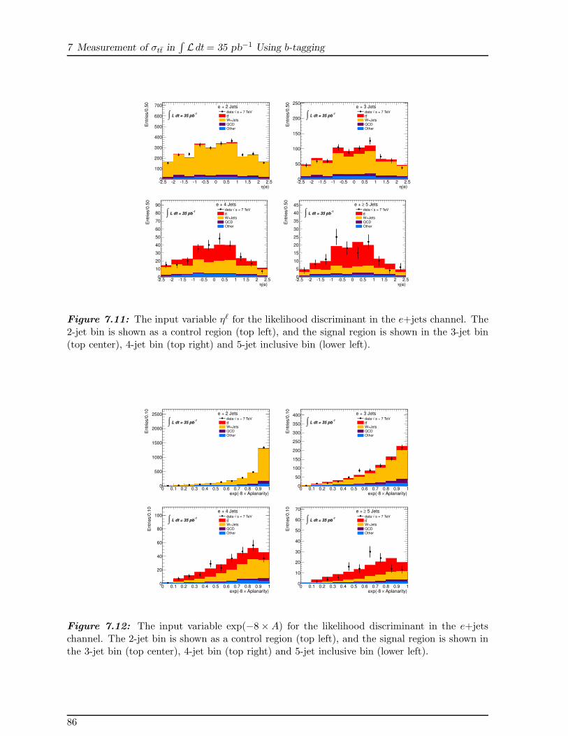
7 Measurement of σtt in∫
L dt= 35 pb−1 Using b-tagging
(e)η2.5 2 1.5 1 0.5 0 0.5 1 1.5 2 2.5
En
trie
s/0
.50
0
100
200
300
400
500
600
700
s = 7 TeV√data
ttW+JetsQCDOther
1 L dt = 35 pb∫
e + 2 Jets
(e)η2.5 2 1.5 1 0.5 0 0.5 1 1.5 2 2.5
En
trie
s/0
.50
0
50
100
150
200
250
s = 7 TeV√data
ttW+JetsQCDOther
1 L dt = 35 pb∫
e + 3 Jets
(e)η2.5 2 1.5 1 0.5 0 0.5 1 1.5 2 2.5
En
trie
s/0
.50
0
10
20
30
40
50
60
70
80
90 s = 7 TeV√data
ttW+JetsQCDOther
1 L dt = 35 pb∫
e + 4 Jets
(e)η2.5 2 1.5 1 0.5 0 0.5 1 1.5 2 2.5
En
trie
s/0
.50
0
5
10
15
20
25
30
35
40
45 s = 7 TeV√data
ttW+JetsQCDOther
1 L dt = 35 pb∫
5 Jets≥e +
Figure 7.11: The input variable ηℓ for the likelihood discriminant in the e+jets channel. The2-jet bin is shown as a control region (top left), and the signal region is shown in the 3-jet bin(top center), 4-jet bin (top right) and 5-jet inclusive bin (lower left).
Aplanarity)×exp(8 0 0.1 0.2 0.3 0.4 0.5 0.6 0.7 0.8 0.9 1
En
trie
s/0
.10
0
500
1000
1500
2000
2500 s = 7 TeV√data
ttW+JetsQCDOther
1 L dt = 35 pb∫
e + 2 Jets
Aplanarity)×exp(8 0 0.1 0.2 0.3 0.4 0.5 0.6 0.7 0.8 0.9 1
En
trie
s/0
.10
0
50
100
150
200
250
300
350
400 s = 7 TeV√data
ttW+JetsQCDOther
1 L dt = 35 pb∫
e + 3 Jets
Aplanarity)×exp(8 0 0.1 0.2 0.3 0.4 0.5 0.6 0.7 0.8 0.9 1
En
trie
s/0
.10
0
20
40
60
80
100 s = 7 TeV√data
ttW+JetsQCDOther
1 L dt = 35 pb∫
e + 4 Jets
Aplanarity)×exp(8 0 0.1 0.2 0.3 0.4 0.5 0.6 0.7 0.8 0.9 1
En
trie
s/0
.10
0
10
20
30
40
50
60
70
s = 7 TeV√data
ttW+JetsQCDOther
1 L dt = 35 pb∫
5 Jets≥e +
Figure 7.12: The input variable exp(−8 ×A) for the likelihood discriminant in the e+jetschannel. The 2-jet bin is shown as a control region (top left), and the signal region is shown inthe 3-jet bin (top center), 4-jet bin (top right) and 5-jet inclusive bin (lower left).
86

7.4 Results of the Fit and Systematic Uncertainties
Ht3p)×exp(40 0.2 0.4 0.6 0.8 1
En
trie
s/0
.10
0
50
100
150
200
250
300
350
400
s = 7 TeV√data
ttW+JetsQCDOther
1 L dt = 35 pb∫
e + 3 Jets
Ht3p)×exp(40 0.2 0.4 0.6 0.8 1
En
trie
s/0
.10
0
20
40
60
80
100 s = 7 TeV√data
ttW+JetsQCDOther
1 L dt = 35 pb∫
e + 4 Jets
Ht3p)×exp(40 0.2 0.4 0.6 0.8 1
En
trie
s/0
.10
0
10
20
30
40
50 s = 7 TeV√data
ttW+JetsQCDOther
1 L dt = 35 pb∫
5 Jets≥e +
Figure 7.13: The input variable exp(−4 ×HT,3p) for the likelihood discriminant in the e+jetschannel. By definition the variable can only be constructed in events with 3 or more jets. Thesignal region is shown in the 3-jet bin (left), 4-jet bin (center) and 5-jet inclusive bin (right).
JPw0 2 4 6 8 10 12 14
En
trie
s/0
.50
0
200
400
600
800
1000
1200
1400 s = 7 TeV√data
ttW+JetsQCDOther
1 L dt = 35 pb∫
e + 2 Jets
JPw0 2 4 6 8 10 12 14
En
trie
s/0
.50
0
50
100
150
200
250
300 s = 7 TeV√data
ttW+JetsQCDOther
1 L dt = 35 pb∫
e + 3 Jets
JPw0 2 4 6 8 10 12 14
En
trie
s/0
.50
0
10
20
30
40
50
60
70
80
90 s = 7 TeV√data
ttW+JetsQCDOther
1 L dt = 35 pb∫
e + 4 Jets
JPw0 2 4 6 8 10 12 14
En
trie
s/0
.50
0
5
10
15
20
25
30
s = 7 TeV√data
ttW+JetsQCDOther
1 L dt = 35 pb∫
5 Jets≥e +
Figure 7.14: The input variable wJP for the likelihood discriminant in the e+jets channel.The 2-jet bin is shown as a control region (top left), and the signal region is shown in the 3-jetbin (top center), 4-jet bin (top right) and 5-jet inclusive bin (lower left).
87

The Difference. “How could you choose avoiding a little pain over understanding a magiclightning machine?”[19]

8 Measurement of σtt in∫
L dt = 0.7 fb−1
Without b-tagging
In the first half of 2011 the LHC continued to deliver proton-proton collisions at an ever increas-ing rate. When the time came to define the datasets to be used for the summer conferences,∫
L dt = 0.7 fb−1 of analyzable data had been recorded, a 20× increase in data compared tothe 2010 dataset analyzed in the previous chapter. The analysis described in Chapter 7 servedas the basis for a similar analysis with this increased dataset. In principle the number of eventsscales directly with luminosity, but changing cuts and conditions can reduce the yield in the finalselected sample. In the e+jets channel the electron trigger threshold was raised as discussedin Section 4.2, necessitating raising the cut on electron pT from 20 to 25 GeV. Furthermore,a large dead region in the calorimeter caused by a hardware malfunction necessitated certainadditional cuts, leading to undesirable asymmetries in the detector and selection. This also ledto increased systematic uncertainties, as have been discussed in Section 4.1. On the acceleratorside, the higher pileup environment increases certain object systematic uncertainties, JES inparticular, as well as increasing the uncertainty on the luminosity determination. The maindifference in this analysis, apart from the hugely increased dataset, is that the b-tagging distri-bution is not used in the discriminant likelihood, but rather the transverse momentum of theleading jet is used instead. This choice makes the analysis highly insensitive to flavor effects,including the assumption that a top quark always decays as t→Wb. The treatment is otherwisevery similar but sensitivity to certain uncertainties naturally changes due to the changing of thisinput variable.
8.1 Selection
In order to be consistent with a tt final state, events are selected which have a lepton, multiplejets and large missing energy, summarized in Section 4.3. The modeling of processes expectedto contribute to the data selected was discussed in Chapter 5. In this analysis, the W+jetscontribution in each jet bin is normalized to a result from the collaboration which exploits thecharge asymmetry in W production at the LHC, and the heavy flavor content is normalized tomeasurements with the same dataset, although this analysis is relatively insensitive to flavor.The QCD multijet contribution is estimated using the matrix method. The predictions andyields are shown in Table 8.1. The uncertainty for QCD is taken from the matrix method, whilein other cases the uncertainty shown is purely statistical. The predictions for basic kinematicdistributions are compared with this dataset in Appendix D.
8.2 The Input Distribution
The analysis uses TMVA to form a likelihood discriminant optimized to separate signal, tt inthe lepton+jets channel, from its main background, W+jets. This is the same procedure as isdescribed in Section 7.2. While this analysis is designed to be flavor insensitive, W+jets includes
89

8 Measurement of σtt in∫
L dt = 0.7 fb−1 Without b-tagging
µ+jets Channel 1 Jet 2 Jet 3 Jet 4 Jet ≥ 5 jet
tt 319± 18 1342± 37 2734± 52 2714± 52 2030± 45W+jets (DD) 383200± 600 93440± 310 20140± 140 4644± 68 1082± 33QCD multijet (DD) 25000± 12000 11000± 6000 3200± 1600 900± 400 290± 150Single Top 996± 32 1148± 34 594± 24 210± 15 84± 9Z+jets 17270± 130 5492± 74 1510± 39 436± 21 149± 12Diboson (WW ,WZ,ZZ) 1093± 33 1009± 32 308± 18 69± 8 18± 4
Total Predicted 428000± 12000 113000± 6000 28400± 1600 8900± 400 3660± 160Data Observed 433931 111741 28643 8680 3814
e+jets Channel 1 Jet 2 Jet 3 Jet 4 Jet ≥ 5 jet
tt 225± 15 1005± 32 1934± 44 1835± 43 1463± 38W+jets(DD) 161600± 400 43170± 210 10840± 100 2486± 50 1032± 32QCD multijet (DD) 11000± 5000 4800± 2400 1600± 800 510± 250 177± 89Single Top 571± 24 711± 27 391± 20 156± 13 65± 8Z+jets 3732± 61 2444± 49 996± 32 333± 18 146± 12Diboson (WW ,WZ,ZZ) 599± 25 538± 23 178± 13 45± 7 10± 3
Total Predicted 177000± 5000 52600± 2400 15900± 800 5360± 260 2892± 100Data Observed 179469 51820 15614 5398 2812
Table 8.1: The yields in both lepton channels for MC predictions and observed data for the∫
L dt = 0.7 fb−1 analysis. Uncertainties are purely statistical except for the QCD multijetprediction, whose uncertainty is taken from the matrix method.
all contributions from the various flavor components available in order to better estimate smallerkinematic differences which can arise when aW is produced along with different flavors of quarks.
The Input Variables
The likelihood discriminator takes four variables as input. Three of the variables are exactlyas they have been described in Section 7.2: the transformed Aplanarity A, the transformednormalized transverse momentum of the event HT,3p, and the lepton pseudorapidity η. Thefourth variable used in this analysis is the transverse momentum of the leading jet, P J1
T . Thevariables HT,3p and P J1
T are not redundant: the numerator of HT,3p is a sum over the pT of thethird and fourth jets only, i.e. the leading jet in the event does not enter by construction. Theleading jet in tt is expected to be harder than the leading jet in W+jets on average. This arisesdue to the distinct production mechanism. The leading jet in tt is generally a b-jet from the topdecaying as t → Wb. The P J1
T spectrum in tt events peaks at a ∼ 1/2×mtop, as can be see inFigures 8.8 and 8.12.
The four variables can be seen in both signal and control regions for µ+jets in Figures 8.7-8.10and similarly for e+jets in Figures 8.11-8.14, found at the end of this chapter. One can see inthese plots a general data-MC agreement. The separation of the discriminant in each of the sixphysics channels can be seen in Figure 8.1, where the signal and background are each normalizedto unity. The shape of the tt signal can be seen to be similar in the six channels, due to therelatively constant amount of signal present and similar separation power. The likelihood beforefitting can be seen as well in Figure 8.2 with both predictions and data shown. Here, too, one
90
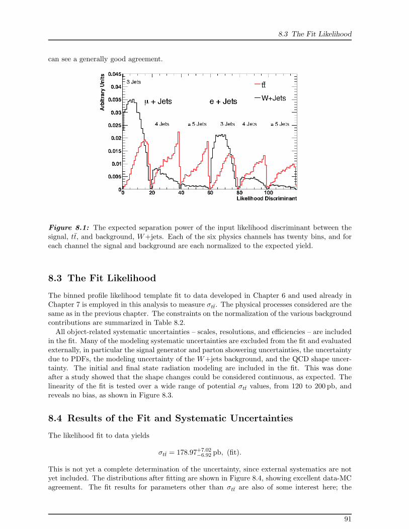
8.3 The Fit Likelihood
can see a generally good agreement.
Figure 8.1: The expected separation power of the input likelihood discriminant between thesignal, tt, and background, W+jets. Each of the six physics channels has twenty bins, and foreach channel the signal and background are each normalized to the expected yield.
8.3 The Fit Likelihood
The binned profile likelihood template fit to data developed in Chapter 6 and used already inChapter 7 is employed in this analysis to measure σtt. The physical processes considered are thesame as in the previous chapter. The constraints on the normalization of the various backgroundcontributions are summarized in Table 8.2.
All object-related systematic uncertainties – scales, resolutions, and efficiencies – are includedin the fit. Many of the modeling systematic uncertainties are excluded from the fit and evaluatedexternally, in particular the signal generator and parton showering uncertainties, the uncertaintydue to PDFs, the modeling uncertainty of the W+jets background, and the QCD shape uncer-tainty. The initial and final state radiation modeling are included in the fit. This was doneafter a study showed that the shape changes could be considered continuous, as expected. Thelinearity of the fit is tested over a wide range of potential σtt values, from 120 to 200 pb, andreveals no bias, as shown in Figure 8.3.
8.4 Results of the Fit and Systematic Uncertainties
The likelihood fit to data yields
σtt = 178.97+7.02−6.92 pb, (fit).
This is not yet a complete determination of the uncertainty, since external systematics are notyet included. The distributions after fitting are shown in Figure 8.4, showing excellent data-MCagreement. The fit results for parameters other than σtt are also of some interest here; the
91

8 Measurement of σtt in∫
L dt = 0.7 fb−1 Without b-tagging
Likelihood Discriminant0 0.1 0.2 0.3 0.4 0.5 0.6 0.7 0.8 0.9 1
Even
ts / 0
.05
0
500
1000
1500
2000
2500
3000 = 7 TeVsData 2011,
tt
W+Jets
QCD Multijet
Z+Jets
Single Top
Diboson
1 L dt = 0.7fb∫
Likelihood Discriminant0 0.1 0.2 0.3 0.4 0.5 0.6 0.7 0.8 0.9 1
Even
ts / 0
.05
0
100
200
300
400
500
600
700
800
900 = 7 TeVsData 2011,
tt
W+Jets
QCD Multijet
Z+Jets
Single Top
Diboson
1 L dt = 0.7fb∫
Likelihood Discriminant0 0.1 0.2 0.3 0.4 0.5 0.6 0.7 0.8 0.9 1
Even
ts / 0
.05
0
100
200
300
400
500 = 7 TeVsData 2011,
tt
W+Jets
QCD Multijet
Z+Jets
Single Top
Diboson
1 L dt = 0.7fb∫
Likelihood Discriminant0 0.1 0.2 0.3 0.4 0.5 0.6 0.7 0.8 0.9 1
Even
ts / 0
.05
0
200
400
600
800
1000
1200
1400
1600
1800 = 7 TeVsData 2011,
tt
W+Jets
QCD Multijet
Z+Jets
Single Top
Diboson
1 L dt = 0.7fb∫
Likelihood Discriminant0 0.1 0.2 0.3 0.4 0.5 0.6 0.7 0.8 0.9 1
Even
ts / 0
.05
0
100
200
300
400
500
= 7 TeVsData 2011,
tt
W+Jets
QCD Multijet
Z+Jets
Single Top
Diboson
1 L dt = 0.7fb∫
Likelihood Discriminant0 0.1 0.2 0.3 0.4 0.5 0.6 0.7 0.8 0.9 1
Even
ts / 0
.05
0
50
100
150
200
250
300 = 7 TeVsData 2011,
tt
W+Jets
QCD Multijet
Z+Jets
Single Top
Diboson
1 L dt = 0.7fb∫
Figure 8.2: The likelihood discriminant for MC and data before the fit. The top row is µ+jets,the bottom row is e+jets. The left hand column is 3-jet exclusive, middle is 4-jet exclusive, andright-most in 5-jet inclusive.
Parameter Constraint
β(tt) noneβ(W→ l + 3 jets) 0.42β(W→ l + 4 jets) 0.48β(W→ l + 5 or more jets) 0.54β(Z+jets) 0.01β(Single top) 0.107β(Diboson) 0.06β(QCD in l + N jets) 0.5
Table 8.2: The input constraints on the various samples. Here, l is either e or µ, and “N jets”is all three jet bins, i.e. 3 exclusive, 4 exclusive, and 5 inclusive.
complete fit results are shown in Table 8.3. The β values returned by the fit for the variousW+jets processes are entirely consistent with the values used to normalize the samples. Thenormalization of the QCD processes returned by the fit vary widely, which is not surprisinggiven the difficulty of determining the normalization. The results are consistent with the inputuncertainty. The profile likelihood is perfectly smooth near its minimum for the parameter ofinterest, shown in Figure 8.5.
92

8.4 Results of the Fit and Systematic Uncertainties
[pb]tt
σInput 120 140 160 180 200
[p
b]
ttσ
Fitte
d
120
140
160
180
200
Fit Linearity
/ ndf 2χ 3.962 / 7
p0 0.437± 0.190
p1 0.003± 0.996
/ ndf 2χ 3.962 / 7
p0 0.437± 0.190
p1 0.003± 0.996
Figure 8.3: The linearity of the fit is tested over the range of input σtt values [120,200] pb insteps of 10 pb. No significant bias is observed.
In many cases the fit is able to constrain the uncertainty from a given systematic source,for instance ISR/FSR are constrained to ∼ 20 % of their original size. Every value returnedis consistent with the envelope given by the combined performance groups, δ=0±1. In somecases, the result is not consistent with the nominal value in the MC. As an example, the valuefor Perugia JES at the likelihood’s minimum is -0.86± 0.17: the fit prefers something muchcloser to the down-shifted systematic uncertainty than the nominal. This does not constitute ameasurement of the uncertainty but rather a constraint from a global fit in a portion of phasespace. Nonetheless, experience has shown that the fit points us in the right direction when thevalue for a δ at the likelihood’s minimum is far from its nominal1.
The correlation of all of the parameters of interest in the fit can be seen in Figure 8.6. Theobserved correlations are generally as expected. The W+jets parameters are correlated to oneanother within a given lepton channel, and the QCD parameter for a given physics channelis anti-correlated to the W+jets component in that same channel. Various correlations existamongst the various JES parameters, which is not surprising given that the same objects are
1The best example comes from a moment when we were testing the fitter for the analysis in the previous chapter.The fit preferred a value for JER of almost exactly δ =-1, thought by us to be interesting but of no particularimportance at the time. Within a few days, it was shown that the resolution of jets in MC does not agreewith that in data, and it was officially recommended that the jet pT should be smeared in the MC, and newsmaller uncertainties were provided.
93
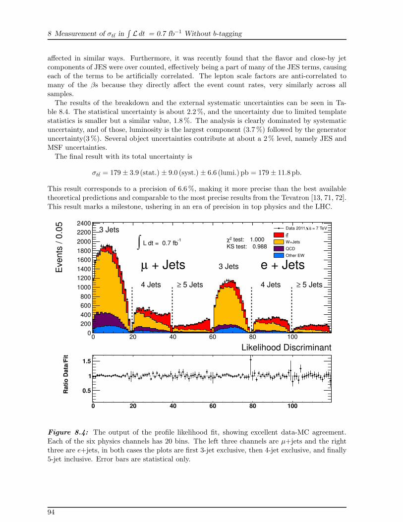
8 Measurement of σtt in∫
L dt = 0.7 fb−1 Without b-tagging
affected in similar ways. Furthermore, it was recently found that the flavor and close-by jetcomponents of JES were over counted, effectively being a part of many of the JES terms, causingeach of the terms to be artificially correlated. The lepton scale factors are anti-correlated tomany of the βs because they directly affect the event count rates, very similarly across allsamples.
The results of the breakdown and the external systematic uncertainties can be seen in Ta-ble 8.4. The statistical uncertainty is about 2.2 %, and the uncertainty due to limited templatestatistics is smaller but a similar value, 1.8 %. The analysis is clearly dominated by systematicuncertainty, and of those, luminosity is the largest component (3.7 %) followed by the generatoruncertainty(3 %). Several object uncertainties contribute at about a 2% level, namely JES andMSF uncertainties.
The final result with its total uncertainty is
σtt = 179 ± 3.9 (stat.) ± 9.0 (syst.) ± 6.6 (lumi.) pb = 179 ± 11.8 pb.
This result corresponds to a precision of 6.6 %, making it more precise than the best availabletheoretical predictions and comparable to the most precise results from the Tevatron [13, 71, 72].This result marks a milestone, ushering in an era of precision in top physics and the LHC.
Likelihood Discriminant
0 20 40 60 80 100
Eve
nts
/ 0
.05
0
200
400
600
800
1000
1200
1400
1600
1800
2000
2200
2400
KS test:0.988
test:1.0002χ1 L dt = 0.7 fb∫
= 7 TeVsData 2011,
tt
W+Jets
QCD
Other EW
3 Jets
4 Jets 5 Jets≥
3 Jets
4 Jets 5 Jets≥
e + Jets + Jetsµ
0 20 40 60 80 100
Ra
tio
Da
ta/F
it
0.5
1
1.5
Figure 8.4: The output of the profile likelihood fit, showing excellent data-MC agreement.Each of the six physics channels has 20 bins. The left three channels are µ+jets and the rightthree are e+jets, in both cases the plots are first 3-jet exclusive, then 4-jet exclusive, and finally5-jet inclusive. Error bars are statistical only.
94

8.4 Results of the Fit and Systematic Uncertainties
Parameter Value Error Error Up Error Down
β(tt) 1.0875 0.0432 0.0427 −0.0421β(W in µ + 3 jets) 0.9738 0.0687 0.0710 −0.0684β(W in µ + 4 jets) 0.8649 0.1026 0.1083 −0.1061β(W in µ + 5 jets) 0.9114 0.1557 0.1589 −0.1510β(W in e + 3 jets) 1.0510 0.0555 0.0597 −0.0588β(W in e + 4 jets) 1.0376 0.0987 0.1057 −0.1025β(W in e + 5 jets) 0.8296 0.1206 0.1267 −0.1257β(Z+jets) 0.9572 0.2604 0.2745 −0.2728β(Single top) 1.0052 0.1066 0.1069 −0.1065β(Diboson) 1.0037 0.0620 0.0620 −0.0620β(QCD in µ + 3 jets) 1.2376 0.2928 0.3307 −0.3426β(QCD in µ + 4 jets) 1.2720 0.3730 0.4234 −0.4152β(QCD in µ + 5 jets) 0.8291 0.3861 0.4044 −0.4095β(QCD in e + 3 jets) 0.6113 0.2157 0.2286 −0.2339β(QCD in e + 4 jets) 0.6152 0.3195 0.3406 −0.3462β(QCD in e + 5 jets) 0.4164 0.3984 0.4221 −0.4170
δ(AlpgenJES) 0.4155 0.4143 0.2725 −0.4030δ(bJES) 0.0964 0.6818 0.5956 −0.6241δ(CaloJES) 0.0051 0.4264 0.3410 −0.3654δ(NoiseJES) −0.3515 0.3979 0.5469 −0.3047δ(PerugiaJES) −0.8653 0.1734 0.1824 −0.1397δ(EtaJES) −0.1943 0.2129 0.2166 −0.1978δ(PileupJES low pT/central) 0.5219 0.1669 0.1539 −0.1633δ(PileupJES low pT/forward) 0.4685 0.2566 0.2361 −0.2791δ(PileupJES high pT/central) 0.6366 0.4684 0.3133 −0.4291δ(PileupJES high pT/forward) 0.0430 0.9105 0.6602 −0.6345δ(Jet Efficiency) 0.1998 0.1357 0.1345 −0.1344δ(JER) 0.1752 0.9544 0.9510 −0.9565δ(FSR) 0.0661 0.2086 0.1897 −0.2239δ(ISR) 0.3392 0.1978 0.1801 −0.2263δ(µ SFs) 0.0923 0.8187 0.7793 −0.7362δ(µ Momentum Smearing at MS) −0.1197 0.8364 0.7873 −0.8234δ(µ Momentum Smearing at ID) −0.2356 0.9337 0.9757 −0.8533δ(µ Energy Scale) 0.0437 1.0838 1.0485 −0.9946δ(e SFs) −0.2300 0.9290 0.9152 −0.8999δ(e Resolution Smearing) 0.3176 0.7668 0.6538 −0.7566δ(e Energy Scale) −0.7455 0.5967 0.7997 −0.5331δ(Emiss
TLAr) 0.0605 0.5062 0.5167 −0.5230
δ(Emiss
Tcellout+softjet) 0.4466 0.4641 0.3333 −0.6785
Table 8.3: The full results of the fit for ~β and ~δ including their uncertainties. The asymmetricerrors are from the minimum of the fit, while the symmetric errors are from the hessian errormatrix..
95
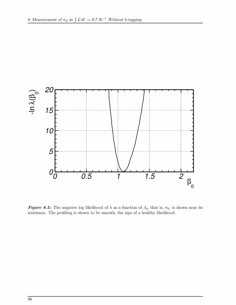
8 Measurement of σtt in∫
L dt = 0.7 fb−1 Without b-tagging
0β
0 0.5 1 1.5 2
)0β(λ
ln
0
5
10
15
20
Figure 8.5: The negative log likelihood of λ as a function of β0, that is, σtt is shown near itsminimum. The profiling is shown to be smooth, the sign of a healthy likelihood.
96

8.4 Results of the Fit and Systematic Uncertainties
1
0.5
0
0.5
1
)t(tβ
+ 3
je
ts)
µ→
(Wβ +
4 je
ts)
µ→
(Wβ +
5 je
ts)
µ→
(Wβ e
+ 3
je
ts)
→(Wβ
e +
4 je
ts)
→(Wβ
e +
5 je
ts)
→(Wβ
(Z+
Je
ts)
β(S
ing
le t
op
)β
(Dib
oso
n)
β +
3 je
ts)
µ(Q
CD
in
β
+ 4
je
ts)
µ(Q
CD
in
β
+ 5
je
ts)
µ(Q
CD
in
β
(QC
D in
e +
3 je
ts)
β (QC
D in
e +
4 je
ts)
β (QC
D in
e +
5 je
ts)
β(A
lpg
en
JE
S)
δ(b
JE
S)
δ(C
alo
JE
S)
δ (No
ise
JE
S)
δ (Pe
rug
iaJE
S)
δ(E
taJE
S)
δ/c
en
tra
l)T
(Pile
up
JE
S lo
w p
δ/f
orw
ard
)T
(Pile
up
JE
S lo
w p
δ/c
en
tra
l)T
(Pile
up
JE
S h
igh
pδ
/fo
rwa
rd)
T(P
ileu
pJE
S h
igh
pδ
(Je
t E
ffic
ien
cy)
δ(J
ER
)δ (F
SR
)δ
(IS
R)
δ SF
s)
µ(δ S
me
arin
g M
S)
T p
µ(δ S
me
arin
g I
D)
T p
µ(δ
En
erg
y S
ca
le)
µ(δ(e
SF
s)
δ(e
Re
so
lutio
n S
me
arin
g)
δ(e
En
erg
y S
ca
le)
δ L
Ar)
T(M
issin
g E
δ S
oft
Je
t)T
(Mis
sin
g E
δ)t(tβ
+ 3 jets)µ→(Wβ + 4 jets)µ→(Wβ + 5 jets)µ→(Wβ
e + 3 jets)→(Wβ e + 4 jets)→(Wβ e + 5 jets)→(Wβ
(Z+Jets)β(Single top)β
(Diboson)β + 3 jets)µ(QCD in β + 4 jets)µ(QCD in β + 5 jets)µ(QCD in β
(QCD in e + 3 jets)β(QCD in e + 4 jets)β(QCD in e + 5 jets)β
(AlpgenJES)δ(bJES)δ
(CaloJES)δ(NoiseJES)δ
(PerugiaJES)δ(EtaJES)δ/central)
T(PileupJES low pδ
/forward)T
(PileupJES low pδ/central)
T(PileupJES high pδ
/forward)T
(PileupJES high pδ(Jet Efficiency)δ
(JER)δ(FSR)δ(ISR)δ SFs)µ(δ
Smearing MS)T
pµ(δ Smearing ID)
T pµ(δ
Energy Scale)µ(δ(e SFs)δ
(e Resolution Smearing)δ(e Energy Scale)δ
LAr)T
(Missing Eδ SoftJet)
T(Missing Eδ
Figure 8.6: The observed correlation of parameters in the fit. Correlations are generally asexpected.
97

8 Measurement of σtt in∫
L dt = 0.7 fb−1 Without b-tagging
Uncertainty up (pb) down (pb) up (%) down (%)
Fit 7.0 6.9 3.9 3.8
Breakdown
Statistical 3.9 −3.9 2.2 −2.2Jets 3.2 −4.3 1.8 −2.4Muon 4.1 −4.1 2.3 −2.3Electron 2.7 −3.0 1.5 −1.7Emiss
T 2.0 −1.6 1.1 −0.9ISR/FSR 3.0 −2.3 1.7 −1.3
External
Generator 5.4 −5.4 3.0 −3.0Hadronization 0.9 −0.9 0.5 −0.5PDF 1.8 −1.8 1.0 −1.0QCD shape 0.7 −0.7 0.4 −0.4W shape 0.9 −0.9 0.5 −0.5Template statistics 3.2 −3.2 1.8 −1.8
Systematic 9.0 −9.0 5.0 −5.0Stat. + syst. 9.8 −9.8 5.4 −5.4
Luminosity 6.6 −6.6 3.7 −3.7
Total 11.8 −11.8 6.6 −6.6
Table 8.4: Estimated uncertainties affecting the σtt measurement. A complete list of sytematicuncertainties considered can be found in Appendix A
98

8.4 Results of the Fit and Systematic Uncertainties
)µ(η2.5 2 1.5 1 0.5 0 0.5 1 1.5 2 2.5
Eve
nts
/ 0
.25
0
5000
10000
15000
20000
25000
30000
35000
40000 = 7 TeVsData 2011,
tt
W+Jets
QCD Multijet
Z+Jets
Single Top
Diboson
1 L dt = 0.7 fb∫+ 1 Jetµ
)µ(η2.5 2 1.5 1 0.5 0 0.5 1 1.5 2 2.5
Eve
nts
/ 0
.25
0
2000
4000
6000
8000
10000
12000
14000
16000 = 7 TeVsData 2011,
tt
W+Jets
QCD Multijet
Z+Jets
Single Top
Diboson
1 L dt = 0.7 fb∫+ 2 Jetsµ
)µ(η2.5 2 1.5 1 0.5 0 0.5 1 1.5 2 2.5
Eve
nts
/ 0
.25
0
500
1000
1500
2000
2500
3000
3500
4000
4500 = 7 TeVsData 2011,
tt
W+Jets
QCD Multijet
Z+Jets
Single Top
Diboson
1 L dt = 0.7 fb∫+ 3 Jetsµ
)µ(η2.5 2 1.5 1 0.5 0 0.5 1 1.5 2 2.5
Eve
nts
/ 0
.25
0
200
400
600
800
1000 = 7 TeVsData 2011,
tt
W+Jets
QCD Multijet
Z+Jets
Single Top
Diboson
1 L dt = 0.7 fb∫+ 4 Jetsµ
)µ(η2.5 2 1.5 1 0.5 0 0.5 1 1.5 2 2.5
Eve
nts
/ 0
.25
0
200
400
600
800
1000
1200
1400
1600 = 7 TeVsData 2011,
tt
W+Jets
QCD Multijet
Z+Jets
Single Top
Diboson
1 L dt = 0.7 fb∫
4 Jets≥+ µ
)µ(η2.5 2 1.5 1 0.5 0 0.5 1 1.5 2 2.5
Eve
nts
/ 0
.25
0
100
200
300
400
500 = 7 TeVsData 2011,
tt
W+Jets
QCD Multijet
Z+Jets
Single Top
Diboson
1 L dt = 0.7 fb∫
5 Jets≥+ µ
Figure 8.7: The input variable ηℓ for the likelihood discriminant in the µ+jets channel. The 1and 2-jet bins are shown as a control region (top left, top center), and the signal region is shownin the 3-jet bin (top right), 4-jet bin (bottom left), and 5-jet inclusive bin (bottom right). The4-jet inclusive bin is shown as well (bottom center).
(leading jet) [GeV]T
p0 50 100 150 200 250 300 350 400
Eve
nts
/ 1
0 G
eV
0
20
40
60
80
100
120
140
160
180
200
220
310×
= 7 TeVsData 2011,
tt
W+Jets
QCD Multijet
Z+Jets
Single Top
Diboson
1 L dt = 0.7 fb∫+ 1 Jetµ
(leading jet) [GeV]T
p0 50 100 150 200 250 300 350 400
Eve
nts
/ 1
0 G
eV
0
5000
10000
15000
20000
25000
30000
35000
40000 = 7 TeVsData 2011,
tt
W+Jets
QCD Multijet
Z+Jets
Single Top
Diboson
1 L dt = 0.7 fb∫+ 2 Jetsµ
(leading jet) [GeV]T
p0 50 100 150 200 250 300 350 400
Eve
nts
/ 1
0 G
eV
0
1000
2000
3000
4000
5000
6000 = 7 TeVsData 2011,
tt
W+Jets
QCD Multijet
Z+Jets
Single Top
Diboson
1 L dt = 0.7 fb∫+ 3 Jetsµ
(leading jet) [GeV]T
p0 50 100 150 200 250 300 350 400
Eve
nts
/ 1
0 G
eV
0
200
400
600
800
1000
1200
1400 = 7 TeVsData 2011,
tt
W+Jets
QCD Multijet
Z+Jets
Single Top
Diboson
1 L dt = 0.7 fb∫+ 4 Jetsµ
(leading jet) [GeV]T
p0 50 100 150 200 250 300 350 400
Eve
nts
/ 1
0 G
eV
0
200
400
600
800
1000
1200
1400
1600
1800
2000 = 7 TeVsData 2011,
tt
W+Jets
QCD Multijet
Z+Jets
Single Top
Diboson
1 L dt = 0.7 fb∫
4 Jets≥+ µ
(leading jet) [GeV]T
p0 50 100 150 200 250 300 350 400
Eve
nts
/ 1
0 G
eV
0
100
200
300
400
500
600 = 7 TeVsData 2011,
tt
W+Jets
QCD Multijet
Z+Jets
Single Top
Diboson
1 L dt = 0.7 fb∫
5 Jets≥+ µ
Figure 8.8: The transverse momentum of the leading jet, P J1T , in the µ+jets channel. The 1
and 2-jet bins are shown as a control region (top left, top center), and the signal region is shownin the 3-jet bin (top right), 4-jet bin (bottom left), and 5-jet inclusive bin (bottom right). The4-jet inclusive bin is shown as well (bottom center).
99

Aplanarity)×exp(8
0 0.1 0.2 0.3 0.4 0.5 0.6 0.7 0.8 0.9 1
Eve
nts
/ 0
.10
0
20
40
60
80
100
120310×
= 7 TeVsData 2011,
tt
W+Jets
QCD Multijet
Z+Jets
Single Top
Diboson
1 L dt = 0.7 fb∫+ 2 Jetsµ
Aplanarity)×exp(8
0 0.1 0.2 0.3 0.4 0.5 0.6 0.7 0.8 0.9 1
Eve
nts
/ 0
.10
0
2000
4000
6000
8000
10000
12000
14000
16000 = 7 TeVsData 2011,
tt
W+Jets
QCD Multijet
Z+Jets
Single Top
Diboson
1 L dt = 0.7 fb∫+ 3 Jetsµ
Aplanarity)×exp(8
0 0.1 0.2 0.3 0.4 0.5 0.6 0.7 0.8 0.9 1
Eve
nts
/ 0
.10
0
500
1000
1500
2000
2500
3000
3500 = 7 TeVsData 2011,
tt
W+Jets
QCD Multijet
Z+Jets
Single Top
Diboson
1 L dt = 0.7 fb∫+ 4 Jetsµ
Aplanarity)×exp(8
0 0.1 0.2 0.3 0.4 0.5 0.6 0.7 0.8 0.9 1
Eve
nts
/ 0
.10
0
1000
2000
3000
4000
5000 = 7 TeVsData 2011,
tt
W+Jets
QCD Multijet
Z+Jets
Single Top
Diboson
1 L dt = 0.7 fb∫
4 Jets≥+ µ
Aplanarity)×exp(8
0 0.1 0.2 0.3 0.4 0.5 0.6 0.7 0.8 0.9 1
Eve
nts
/ 0
.10
0
200
400
600
800
1000
1200
1400 = 7 TeVsData 2011,
tt
W+Jets
QCD Multijet
Z+Jets
Single Top
Diboson
1 L dt = 0.7 fb∫
5 Jets≥+ µ
Figure 8.9: The transformed Aplanarity of the event, A, in the µ+jets channel. The 2-jetbin is shown as a control region (top left), and the signal region is shown in the 3-jet bin (topcenter), 4-jet bin (top right), and 5-jet inclusive bin (bottom right). The 4-jet inclusive bin isshown as well (bottom left).
)Tp,3 H×exp(4 0 0.1 0.2 0.3 0.4 0.5 0.6 0.7 0.8 0.9 1
Eve
nts
/ 0
.10
0
2000
4000
6000
8000
10000
12000
14000
16000 = 7 TeVsData 2011,
tt
W+Jets
QCD Multijet
Z+Jets
Single Top
Diboson
1 L dt = 0.7 fb∫+ 3 Jetsµ
)Tp,3 H×exp(4 0 0.1 0.2 0.3 0.4 0.5 0.6 0.7 0.8 0.9 1
Eve
nts
/ 0
.10
0
500
1000
1500
2000
2500
3000
3500
4000 = 7 TeVsData 2011,
tt
W+Jets
QCD Multijet
Z+Jets
Single Top
Diboson
1 L dt = 0.7 fb∫+ 4 Jetsµ
)Tp,3 H×exp(4 0 0.1 0.2 0.3 0.4 0.5 0.6 0.7 0.8 0.9 1
Eve
nts
/ 0
.10
0
1000
2000
3000
4000
5000
= 7 TeVsData 2011,
tt
W+Jets
QCD Multijet
Z+Jets
Single Top
Diboson
1 L dt = 0.7 fb∫
4 Jets≥+ µ
)Tp,3 H×exp(4 0 0.1 0.2 0.3 0.4 0.5 0.6 0.7 0.8 0.9 1
Eve
nts
/ 0
.10
0
200
400
600
800
1000
1200
1400
1600 = 7 TeVsData 2011,
tt
W+Jets
QCD Multijet
Z+Jets
Single Top
Diboson
1 L dt = 0.7 fb∫
5 Jets≥+ µ
Figure 8.10: The transformed normalized momentum of the event, HT,3p, in the µ+jetschannel. The signal region is shown in the 3-jet bin (top left), 4-jet bin (top right), and 5-jetinclusive bin (bottom right). The 4-jet inclusive bin is shown as well (bottom left). The variableis not defined for lower jet multiplicity bins.

8.4 Results of the Fit and Systematic Uncertainties
(e)η2.5 2 1.5 1 0.5 0 0.5 1 1.5 2 2.5
Eve
nts
/ 0
.50
0
5000
10000
15000
20000
25000
30000
35000 = 7 TeVsData 2011,
tt
W+Jets
QCD Multijet
Z+Jets
Single Top
Diboson
1 L dt = 0.7 fb∫
e+ 1 Jet
(e)η2.5 2 1.5 1 0.5 0 0.5 1 1.5 2 2.5
Eve
nts
/ 0
.50
0
2000
4000
6000
8000
10000 = 7 TeVsData 2011,
tt
W+Jets
QCD Multijet
Z+Jets
Single Top
Diboson
1 L dt = 0.7 fb∫
e+ 2 Jets
(e)η2.5 2 1.5 1 0.5 0 0.5 1 1.5 2 2.5
Eve
nts
/ 0
.50
0
500
1000
1500
2000
2500
3000
3500
= 7 TeVsData 2011,
tt
W+Jets
QCD Multijet
Z+Jets
Single Top
Diboson
1 L dt = 0.7 fb∫
e+ 3 Jets
(e)η2.5 2 1.5 1 0.5 0 0.5 1 1.5 2 2.5
Eve
nts
/ 0
.50
0
200
400
600
800
1000
1200 = 7 TeVsData 2011,
tt
W+Jets
QCD Multijet
Z+Jets
Single Top
Diboson
1 L dt = 0.7 fb∫
e+ 4 Jets
(e)η2.5 2 1.5 1 0.5 0 0.5 1 1.5 2 2.5
Eve
nts
/ 0
.50
0
200
400
600
800
1000
1200
1400
1600
1800 = 7 TeVsData 2011,
tt
W+Jets
QCD Multijet
Z+Jets
Single Top
Diboson
1 L dt = 0.7 fb∫
4 Jets≥e+
(e)η2.5 2 1.5 1 0.5 0 0.5 1 1.5 2 2.5
Eve
nts
/ 0
.50
0
100
200
300
400
500
600
700 = 7 TeVsData 2011,
tt
W+Jets
QCD Multijet
Z+Jets
Single Top
Diboson
1 L dt = 0.7 fb∫
5 Jets≥e+
Figure 8.11: The input variable ηℓ for the likelihood discriminant in the e+jets channel. The1 and 2-jet bins are shown as a control region (top left, top center), and the signal region isshown in the 3-jet bin (top right), 4-jet bin (bottom left), and 5-jet inclusive bin (bottom right).The 4-jet inclusive bin is shown as well (bottom center).
(leading jet) [GeV]T
p0 50 100 150 200 250 300 350 400
Eve
nts
/ 1
0 G
eV
0
10000
20000
30000
40000
50000
60000
70000
80000 = 7 TeVsData 2011,
tt
W+Jets
QCD Multijet
Z+Jets
Single Top
Diboson
1 L dt = 0.7 fb∫
e+ 1 Jet
(leading jet) [GeV]T
p0 50 100 150 200 250 300 350 400
Eve
nts
/ 1
0 G
eV
0
2000
4000
6000
8000
10000
12000
14000
16000 = 7 TeVsData 2011,
tt
W+Jets
QCD Multijet
Z+Jets
Single Top
Diboson
1 L dt = 0.7 fb∫
e+ 2 Jets
(leading jet) [GeV]T
p0 50 100 150 200 250 300 350 400
Eve
nts
/ 1
0 G
eV
0
500
1000
1500
2000
2500
3000
= 7 TeVsData 2011,
tt
W+Jets
QCD Multijet
Z+Jets
Single Top
Diboson
1 L dt = 0.7 fb∫
e+ 3 Jets
(leading jet) [GeV]T
p0 50 100 150 200 250 300 350 400
Eve
nts
/ 1
0 G
eV
0
100
200
300
400
500
600
700
800
900
= 7 TeVsData 2011,
tt
W+Jets
QCD Multijet
Z+Jets
Single Top
Diboson
1 L dt = 0.7 fb∫
e+ 4 Jets
(leading jet) [GeV]T
p0 50 100 150 200 250 300 350 400
Eve
nts
/ 1
0 G
eV
0
200
400
600
800
1000
1200 = 7 TeVsData 2011,
tt
W+Jets
QCD Multijet
Z+Jets
Single Top
Diboson
1 L dt = 0.7 fb∫
4 Jets≥e+
(leading jet) [GeV]T
p0 50 100 150 200 250 300 350 400
Eve
nts
/ 1
0 G
eV
0
50
100
150
200
250
300
350
400
450 = 7 TeVsData 2011,
tt
W+Jets
QCD Multijet
Z+Jets
Single Top
Diboson
1 L dt = 0.7 fb∫
5 Jets≥e+
Figure 8.12: The transverse momentum of the leading jet, P J1T , in the e+jets channel. The 1
and 2-jet bins are shown as a control region (top left, top center), and the signal region is shownin the 3-jet bin (top right), 4-jet bin (bottom left), and 5-jet inclusive bin (bottom right). The4-jet inclusive bin is shown as well (bottom center).
101

8 Measurement of σtt in∫
L dt = 0.7 fb−1 Without b-tagging
Aplanarity)×exp(8
0 0.1 0.2 0.3 0.4 0.5 0.6 0.7 0.8 0.9 1
Eve
nts
/ 0
.10
0
10000
20000
30000
40000
50000 = 7 TeVsData 2011,
tt
W+Jets
QCD Multijet
Z+Jets
Single Top
Diboson
1 L dt = 0.7 fb∫
e+ 2 Jets
Aplanarity)×exp(8
0 0.1 0.2 0.3 0.4 0.5 0.6 0.7 0.8 0.9 1
Eve
nts
/ 0
.10
0
1000
2000
3000
4000
5000
6000
7000
8000 = 7 TeVsData 2011,
tt
W+Jets
QCD Multijet
Z+Jets
Single Top
Diboson
1 L dt = 0.7 fb∫
e+ 3 Jets
Aplanarity)×exp(8
0 0.1 0.2 0.3 0.4 0.5 0.6 0.7 0.8 0.9 1
Eve
nts
/ 0
.10
0
200
400
600
800
1000
1200
1400
1600
1800
2000
2200 = 7 TeVsData 2011,
tt
W+Jets
QCD Multijet
Z+Jets
Single Top
Diboson
1 L dt = 0.7 fb∫
e+ 4 Jets
Aplanarity)×exp(8
0 0.1 0.2 0.3 0.4 0.5 0.6 0.7 0.8 0.9 1
Eve
nts
/ 0
.10
0
500
1000
1500
2000
2500
3000 = 7 TeVsData 2011,
tt
W+Jets
QCD Multijet
Z+Jets
Single Top
Diboson
1 L dt = 0.7 fb∫
4 Jets≥e+
Aplanarity)×exp(8
0 0.1 0.2 0.3 0.4 0.5 0.6 0.7 0.8 0.9 1
Eve
nts
/ 0
.10
0
200
400
600
800
1000 = 7 TeVsData 2011,
tt
W+Jets
QCD Multijet
Z+Jets
Single Top
Diboson
1 L dt = 0.7 fb∫
5 Jets≥e+
Figure 8.13: The transformed Aplanarity of the event, A, in the e+jets channel. The 2-jetbin is shown as a control region (top left), and the signal region is shown in the 3-jet bin (topcenter), 4-jet bin (top right), and 5-jet inclusive bin (bottom right). The 4-jet inclusive bin isshown as well (bottom left).
)Tp,3 H×exp(4 0 0.1 0.2 0.3 0.4 0.5 0.6 0.7 0.8 0.9 1
Eve
nts
/ 0
.10
0
1000
2000
3000
4000
5000
6000
7000
8000 = 7 TeVsData 2011,
tt
W+Jets
QCD Multijet
Z+Jets
Single Top
Diboson
1 L dt = 0.7 fb∫
e+ 3 Jets
)Tp,3 H×exp(4 0 0.1 0.2 0.3 0.4 0.5 0.6 0.7 0.8 0.9 1
Eve
nts
/ 0
.10
0
200
400
600
800
1000
1200
1400
1600
1800
2000
2200 = 7 TeVsData 2011,
tt
W+Jets
QCD Multijet
Z+Jets
Single Top
Diboson
1 L dt = 0.7 fb∫
e+ 4 Jets
)Tp,3 H×exp(4 0 0.1 0.2 0.3 0.4 0.5 0.6 0.7 0.8 0.9 1
Eve
nts
/ 0
.10
0
500
1000
1500
2000
2500
3000 = 7 TeVsData 2011,
tt
W+Jets
QCD Multijet
Z+Jets
Single Top
Diboson
1 L dt = 0.7 fb∫
4 Jets≥e+
)Tp,3 H×exp(4 0 0.1 0.2 0.3 0.4 0.5 0.6 0.7 0.8 0.9 1
Eve
nts
/ 0
.10
0
100
200
300
400
500
600
700
800
900 = 7 TeVsData 2011,
tt
W+Jets
QCD Multijet
Z+Jets
Single Top
Diboson
1 L dt = 0.7 fb∫
5 Jets≥e+
Figure 8.14: The transformed normalized momentum of the event, HT,3p, in the e+jets chan-nel. The signal region is shown in the 3-jet bin (top left), 4-jet bin (top right), and 5-jet inclusivebin (bottom right). The 4-jet inclusive bin is shown as well (bottom left). The variable is notdefined for lower jet multiplicity bins.
102


Unscientific. “Last week, we busted the myth that electroweak gauge symmetry is broken bythe Higgs mechanism. We’ll also examine the existence of God and whether true love exists.”[19]

9 Simultaneous Measurement of σtt, fWHF,
and fWc in∫
L dt = 0.7 fb−1
With the formalism developed in Chapter 6 and experience gained throughout the course ofthe analyses presented in Chapters 7 and 8, it is possible to turn to a related analysis in whichotherwise irreducible background contributions to the data are themselves turned into parame-ters of interest in the fit, allowing for a measurement of multiple parameters simultaneously. Inparticular, a single flavor-sensitive distribution is used to measure the top pair production crosssection as well as the ratio of events in which a W boson is produced in association with a pairof heavy quarks (bb or cc) to the events in which a W boson is produced with other jets, fWHF
,and similarly the ratio fWc for a W boson in association with a c or c. These ratios have beendefined in Section 2.3 such that
fWHF·(
σ(W+QQ)incl.
σ(W+2 jets)incl.− σ(W+QQ)incl.
)
MC
=
(
σ(W+QQ)incl.
σ(W+2 jets)incl.− σ(W+QQ)incl.
)
Measured
,
fWc ·(
σ(W+c/c+jet)incl.
σ(W+2 jets)incl.− σ(W+c/c+jet)incl.
)
MC
=
(
σ(W+c/c+jet)incl.
σ(W+2 jets)incl.− σ(W+c/c+jet)incl.
)
Measured
.
They were measured with respect to the MC scaled to the ATLAS data, the default taken in theanalysis in the preceding chapter. Those measurements by the collaboration were fWHF
= 1.63and fWc= 1.11 with respect to the ALPGEN MC cross sections. A result from this analysis offWHF
= fWc= 1.0 would therefore be identical to the ATLAS measurements but not the defaultin the MC.
The discriminant distribution used is based on the output of a b-tagging algorithm whichutilizes a neural network (amongst other techniques) to discriminate amongst b, c, and light jets.The output is used as a continuous distribution, in a similar fashion to the continuous b-taggingvariable used in the
∫
L dt= 35 pb−1 analysis described in Chapter 7. The dataset and selectionused here are identical to those used in Chapter 8, namely the analysis uses
∫
L dt = 0.7 fb−1ofdata collected in 2011 with the selection of both semi-leptonic decay channels, summarized inSection 4.3.
In this analysis the 2-jet bin is used as well. Although the tt contribution is expected to besmall compared to the higher jet multiplicity bins, the W+QQ cross section is expected to peakthere. Similarly, W + c/c is expected to be larger there than in higher bins. Including the 2-jetbin therefore increases the precision of the fWHF
and fWc determinations. The 4 and 5-jet binsare now grouped together as 4-jet inclusive, due to low MC statistics available in the W+jetssamples, especially those containing heavy flavor jets.
Comparison of simulation with observation for basic kinematic distributions in the datasetare shown in Appendix D. Additionaly, for the sake of comparison, the discriminant variablesused in the previous analysis are also shown in the 2-jet exclusive and 4-jet inclusive jet bins, inFigures 8.7-8.14.
105
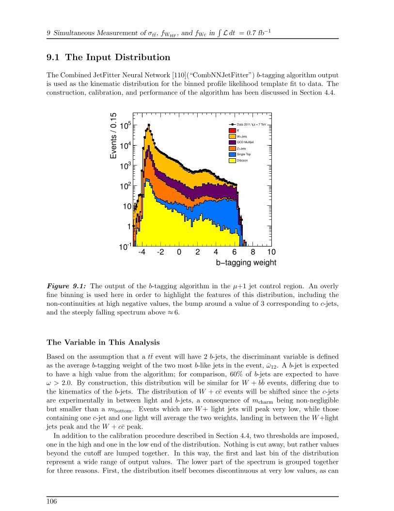
9 Simultaneous Measurement of σtt, fWHF, and fWc in
∫
L dt = 0.7 fb−1
9.1 The Input Distribution
The Combined JetFitter Neural Network [110](“CombNNJetFitter”) b-tagging algorithm outputis used as the kinematic distribution for the binned profile likelihood template fit to data. Theconstruction, calibration, and performance of the algorithm has been discussed in Section 4.4.
b−tagging weight
4 2 0 2 4 6 8 10
Events
/ 0
.15
110
1
10
210
310
410
510 = 7 TeVsData 2011,
tt
W+Jets
QCD Multijet
Z+Jets
Single Top
Diboson
Figure 9.1: The output of the b-tagging algorithm in the µ+1 jet control region. An overlyfine binning is used here in order to highlight the features of this distribution, including thenon-continuities at high negative values, the bump around a value of 3 corresponding to c-jets,and the steeply falling spectrum above ≈ 6.
The Variable in This Analysis
Based on the assumption that a tt event will have 2 b-jets, the discriminant variable is definedas the average b-tagging weight of the two most b-like jets in the event, ω12. A b-jet is expectedto have a high value from the algorithm; for comparison, 60% of b-jets are expected to haveω > 2.0. By construction, this distribution will be similar for W + bb events, differing due tothe kinematics of the b-jets. The distribution of W + cc events will be shifted since the c-jetsare experimentally in between light and b-jets, a consequence of mcharm being non-negligiblebut smaller than a mbottom. Events which are W+ light jets will peak very low, while thosecontaining one c-jet and one light will average the two weights, landing in between the W+lightjets peak and the W + cc peak.
In addition to the calibration procedure described in Section 4.4, two thresholds are imposed,one in the high and one in the low end of the distribution. Nothing is cut away, but rather valuesbeyond the cutoff are lumped together. In this way, the first and last bin of the distributionrepresent a wide range of output values. The lower part of the spectrum is grouped togetherfor three reasons. First, the distribution itself becomes discontinuous at very low values, as can
106

9.2 The Fit Likelihood
be seen at a value of ω ≈ −4.5 in Figure 9.1. This is problematic for fitting. Additionally, thesteeply falling spectrum can contribute to uncertainty due to arbitrary bin thresholds. Lastly,it is clear from the calibration procedure that the very light part (ω ≈ −3) of the spectrum isnot calibrated, and thus is not expected to agree perfectly with predictions. All jets below thelowest working point, ω=-1.25, which corresponds to a b-tagging efficiency of 80 %, have thesame calibration. This rough calibration yields poor MC-data agreement in the low part of thespectrum when viewed in fine bins, but differences average out over the whole low ω range. Onecould consider cutting away the region, however much sensitivity would be lost in the analysis:in addition to the general loss of statistics, most W plus light jet events would be cut away andmany W+c events as well. Thus the lower part of the spectrum is retained in a single bin.
At the high end of the spectrum, above ω= 2.40, which corresponds to a b-tagging efficiencyof 57 %, the events are lumped together for the far simpler reason that statistics begin to runout, in particular in the simulation. The fit needs a modicum of statistics, in particular in eachbin of the templates to perform well. One can compare the distributions before this clumping inFigure 9.1 with those after in Figure 9.2, where the former uses fine binning to show structureand the latter uses the coarse binning used in the fit.
The analysis discriminant is shown in both lepton channels in all three jet bins in Figures 9.2and 9.3. One can see the same distribution in several different forms, namely in logarithmicscale with data overlaid, and the separation power of the three parameters of interest on linearscale, both shown as a complete distribution and zoomed in to show the wide distributionmeaningfully. The W+light jet component, as well the next numerically largest background,Z+jets, are shown as well for comparison.
9.2 The Fit Likelihood
A binned profile likelihood template fit to data is performed, following the method developedin Chapter 6. The specifics of its configuration are described here. The parameters of interestin the likelihood are σtt, fWHF
, and fWc, each of which are unconstrained and fitted as a singleparameter, that is, taken to be the same across all jet bins. While this is self explanatory for toppair production, it requires some justification in the case of heavy flavor associated production.From the arguments developed in Section 2.3, it can be seen that the underlying physics in eachof the jet bins is identical, with an “extra” radiated light jet in the higher bins. The productionmechanism for the heavy flavor contribution overwhelmingly remains the same, regardless ofhow many light jets are produced in the event.
The main background to all of the processes of interest is W+light jet production, which isnormalized in the same way as described in Chapter 8, and taken as a separate parameter ineach jet bin and each channel, with an uncertainty increasing from each jet bin to the nextwithin a given channel. Constraints are the same as in the previous chapter, shown in Table 8.2.
The starting point of this analysis was the inclusion of nearly all systematic uncertaintiesas nuisance parameters in the likelihood. However, the inclusion of nuisance parameters intothe fit for many systematic uncertainties has proved problematic due to the insensitivity ofthe fit variable to them. One can understand clearly that, for example, changing the electronscale factor has no effect on the shape of the b-tagging distribution. Indeed, many systematicuncertainties show a negligible effect on the shape and thus only affect the rate of the processesinvolved. The inclusion of rate-only uncertainties led to non-sensical results in testing. Thus allrate-only uncertainties are removed from the likelihood.
The main object uncertainties affecting the discriminant, the uncertainty on the b-taggingcalibration, are included in the fit as eight separate parameters, as previously. Apart from
107

9 Simultaneous Measurement of σtt, fWHF, and fWc in
∫
L dt = 0.7 fb−1
12ω
1 0 1 2 3 4 5
Eve
nts
1
10
210
310
410
510 data 2011
ttWc
WHFWLF
qcd
Z
singletop
diboson
12ω
1 0 1 2 3 4 5
No
rma
lize
d, A
britr
ary
Units
0
0.2
0.4
0.6
0.8
1
1.2ttWc
WHFWLFZ
12ω
1 0 1 2 3 4 5
No
rma
lize
d, A
britr
ary
Units
0
0.05
0.1
0.15
0.2
0.25
ttWc
WHFWLFZ
ttWc
WHFWLFZ
12ω
1 0 1 2 3 4 5
Eve
nts
1
10
210
310
410
510 data 2011
ttWc
WHFWLF
qcd
Z
singletop
diboson
12ω
1 0 1 2 3 4 5
No
rma
lize
d, A
britr
ary
Units
0
0.2
0.4
0.6
0.8
1
1.2ttWc
WHFWLFZ
12ω
1 0 1 2 3 4 5
No
rma
lize
d, A
britr
ary
Units
0
0.05
0.1
0.15
0.2
0.25
ttWc
WHFWLFZ
ttWc
WHFWLFZ
12ω
1 0 1 2 3 4 5
Eve
nts
1
10
210
310
410
510 data 2011
ttWc
WHFWLF
qcd
Z
singletop
diboson
12ω
1 0 1 2 3 4 5
No
rma
lize
d, A
britr
ary
Units
0
0.2
0.4
0.6
0.8
1
1.2ttWc
WHFWLFZ
12ω
1 0 1 2 3 4 5N
orm
aliz
ed, A
britr
ary
Units
0
0.05
0.1
0.15
0.2
0.25
ttWc
WHFWLFZ
ttWc
WHFWLFZ
Figure 9.2: The input distribution in e+jets. The rows descend in increasing jet bin, beginningwith e+2 jets and ending with e+4 jets (inclusive). The left most column is the input distributionwith eight bins after both high and low cutoffs are applied, as it is used in the fit. The next twocolumns of plots show the expected discriminating power, where each contribution is normalizedto unity so that the shapes can be seen. The central column is the full distribution, while theright most column cuts off the y-axis in order to be able to see more clearly the discriminatingpower in the region which is not dominated by light jets.
these, JES – taken as an envelope – has enough of a shape affect to allow for inclusion. Theother uncertainties which remain as nuisance parameters in the fit are those affecting tt shape,namely the initial and final state radiation (ISR/FSR), the generator, and showering modeling,as described in Section 5. Other uncertainties affecting jets (JER, pileup contribution to JES,and b-JES) yield extremely unsmooth profiling and are thus not included either. Given thegeneral power of the profile likelihood method to constrain uncertainties, the exclusion of manyobject uncertainties is expected to enlarge the overall uncertainty in the analysis with respectto the analysis in the previous chapter, even though the same dataset and prescriptions forsystematic uncertainties are used.
Expected Behavior
The expected behavior of the likelihood is evaluated. Checks include linearity of the fit, cor-relation amongst the parameters of interest, and expected uncertainty from the fit. To checklinearity, varied fractions of each of the three parameters of interest are injected (separately) and
108

9.2 The Fit Likelihood
12ω
1 0 1 2 3 4 5
Eve
nts
1
10
210
310
410
510 data 2011
ttWc
WHFWLF
qcd
Z
singletop
diboson
12ω
1 0 1 2 3 4 5
No
rma
lize
d, A
britr
ary
Units
0
0.2
0.4
0.6
0.8
1
1.2ttWc
WHFWLFZ
12ω
1 0 1 2 3 4 5
No
rma
lize
d, A
britr
ary
Units
0
0.05
0.1
0.15
0.2
0.25
ttWc
WHFWLFZ
ttWc
WHFWLFZ
12ω
1 0 1 2 3 4 5
Eve
nts
1
10
210
310
410
510 data 2011
ttWc
WHFWLF
qcd
Z
singletop
diboson
12ω
1 0 1 2 3 4 5
No
rma
lize
d, A
britr
ary
Units
0
0.2
0.4
0.6
0.8
1
1.2ttWc
WHFWLFZ
12ω
1 0 1 2 3 4 5
No
rma
lize
d, A
britr
ary
Units
0
0.05
0.1
0.15
0.2
0.25
ttWc
WHFWLFZ
ttWc
WHFWLFZ
12ω
1 0 1 2 3 4 5
Eve
nts
1
10
210
310
410
510 data 2011
ttWc
WHFWLF
qcd
Z
singletop
diboson
12ω
1 0 1 2 3 4 5
No
rma
lize
d, A
britr
ary
Units
0
0.2
0.4
0.6
0.8
1
1.2ttWc
WHFWLFZ
12ω
1 0 1 2 3 4 5N
orm
aliz
ed, A
britr
ary
Units
0
0.05
0.1
0.15
0.2
0.25
ttWc
WHFWLFZ
ttWc
WHFWLFZ
Figure 9.3: The input distribution in µ+jets. The rows descend in increasing jet bin, beginningwith µ+2 jets and ending with µ+4 jet (inclusive). The left most column is the input distributionwith eight bins after both high and low cutoffs are applied, as it is used in the fit. The next twocolumns of plots show the expected discriminating power, where each contribution is normalizedto 1 so that the shapes can be seen. The central column is the full distribution, while the rightmost column cuts off the y-axis in order to be able to see more clearly the discriminating powerin the region which is not dominated by light jets.
then fit to check for any possible bias. For σtt the range [120-200] pb is used in steps of 10 pb.For fWHF
and fWc the range [0.4-2.0] is used with steps of 0.2. At each point, 1,000 pseudo-experiments are drawn and the full fit including nuisance parameters is made. The results areshown in Figure 9.5. The test for σtt shows a ∼ 1 % offset, treatment of which will be discussedin the results section. The results for the linearity of fWHF
and fWc are extremely good.
Correlation amongst the various parameters of interest is also expected: one can see fromthe input distributions in Figures 9.2 and 9.3 that σtt and fWHF
should be anti-correlated, andsimilarly fWHF
and fWc. Using a statistics only fit (i.e. without any nuisance parameters),thousands of PEs are drawn, and the result of the fits for each pair of two parameters of interestare plotted against one another, from which the correlation is estimated. This is shown inFigure 9.4. There, an anti-correlation between σtt and fWHF
as well as an anti-correlationbetween fWHF
and fWc are observed using ensemble testing, as naively expected. By transience,there is then an expected correlation between σtt and fWc observed in pseudo-experiment testing.Expected correlations are in the range of 40-75 %. The measured correlation and effects of this
109
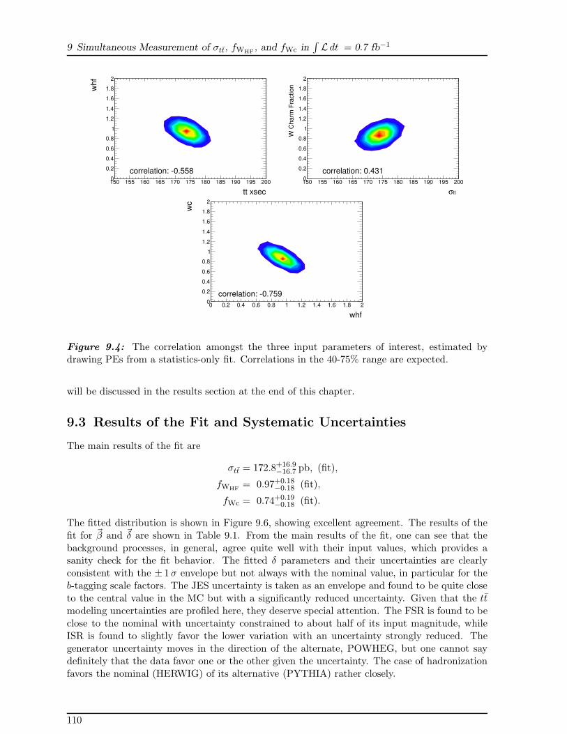
9 Simultaneous Measurement of σtt, fWHF, and fWc in
∫
L dt = 0.7 fb−1
tt xsec
150 155 160 165 170 175 180 185 190 195 200
wh
f
0
0.2
0.4
0.6
0.8
1
1.2
1.4
1.6
1.8
2
correlation: 0.558
ttσ150 155 160 165 170 175 180 185 190 195 200
W C
harm
Fra
ction
0
0.2
0.4
0.6
0.8
1
1.2
1.4
1.6
1.8
2
correlation: 0.431
whf
0 0.2 0.4 0.6 0.8 1 1.2 1.4 1.6 1.8 2
wc
0
0.2
0.4
0.6
0.8
1
1.2
1.4
1.6
1.8
2
correlation: 0.759
Figure 9.4: The correlation amongst the three input parameters of interest, estimated bydrawing PEs from a statistics-only fit. Correlations in the 40-75% range are expected.
will be discussed in the results section at the end of this chapter.
9.3 Results of the Fit and Systematic Uncertainties
The main results of the fit are
σtt = 172.8+16.9−16.7 pb, (fit),
fWHF= 0.97+0.18
−0.18 (fit),
fWc = 0.74+0.19−0.18 (fit).
The fitted distribution is shown in Figure 9.6, showing excellent agreement. The results of thefit for ~β and ~δ are shown in Table 9.1. From the main results of the fit, one can see that thebackground processes, in general, agree quite well with their input values, which provides asanity check for the fit behavior. The fitted δ parameters and their uncertainties are clearlyconsistent with the ± 1σ envelope but not always with the nominal value, in particular for theb-tagging scale factors. The JES uncertainty is taken as an envelope and found to be quite closeto the central value in the MC but with a significantly reduced uncertainty. Given that the ttmodeling uncertainties are profiled here, they deserve special attention. The FSR is found to beclose to the nominal with uncertainty constrained to about half of its input magnitude, whileISR is found to slightly favor the lower variation with an uncertainty strongly reduced. Thegenerator uncertainty moves in the direction of the alternate, POWHEG, but one cannot saydefinitely that the data favor one or the other given the uncertainty. The case of hadronizationfavors the nominal (HERWIG) of its alternative (PYTHIA) rather closely.
110

9.3 Results of the Fit and Systematic Uncertainties
[pb]tt
σInput 120 130 140 150 160 170 180 190 200
[pb]
t tσ
Fitte
d
120
130
140
150
160
170
180
190
200
/ ndf 2χ 5.291 / 7
p0 0.856± 2.309
p1 0.005± 0.984
Input W Heavy Flavor Fraction0.4 0.6 0.8 1 1.2 1.4 1.6 1.8 2
Fitte
d W
Heavy F
lavor
Fra
ction
0.4
0.6
0.8
1
1.2
1.4
1.6
1.8
2
/ ndf 2χ 10.532 / 7
p0 0.005± 0.010
p1 0.004± 0.991
Input W Charm Fraction0.4 0.6 0.8 1 1.2 1.4 1.6 1.8 2
Fitte
d W
Charm
Fra
ction
0.4
0.6
0.8
1
1.2
1.4
1.6
1.8
2
/ ndf 2χ 8.946 / 7
p0 0.005± 0.005
p1 0.005± 0.993
Figure 9.5: The linearity tests with fit results for the σtt, fWHFand fWc analysis. Offsets in
both the linearity and slope of tt are observed and corrected for. The linearity tests for fWHF
and fWc reveal no bias.
111

9 Simultaneous Measurement of σtt, fWHF, and fWc in
∫
L dt = 0.7 fb−1
bTagging Discriminant
0 5 10 15 20 25 30 35 40 45
Eve
nts
210
310
410
510
610
1 L dt = 0.70 fb∫
= 7 TeVsData 2011,
ttW+ light Jets
+ Jetsc/cbW+b + JetscW+c/
QCD Multijet
Other EW
e + Jets + Jetsµ
0 5 10 15 20 25 30 35 40 45
Ra
tio
Da
ta/F
it
0.5
1
1.5
Figure 9.6: The six-channel distribution after the fit, showing excellent data-MC agreement.Each of the six channels has eight bins. Left most are e+2 jets, followed by e+3 jets and e+4jets (inclusive). The µ+jets channels follow. Errors on data points are statistical only.
112
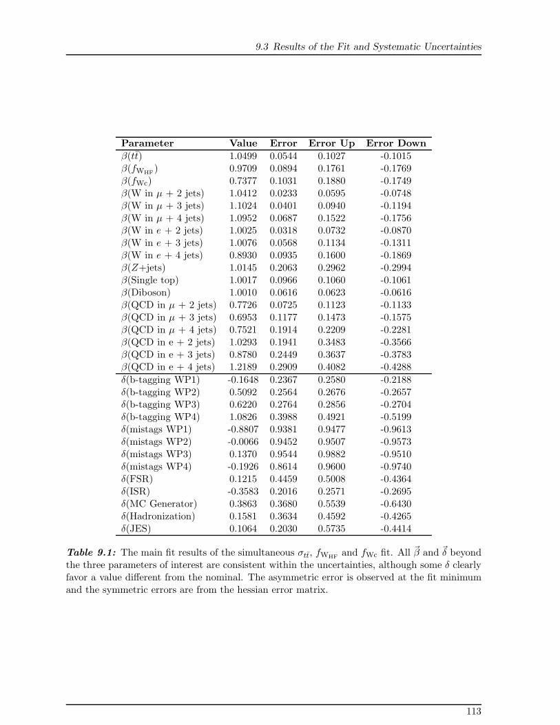
9.3 Results of the Fit and Systematic Uncertainties
Parameter Value Error Error Up Error Down
β(tt) 1.0499 0.0544 0.1027 -0.1015β(fWHF
) 0.9709 0.0894 0.1761 -0.1769β(fWc) 0.7377 0.1031 0.1880 -0.1749β(W in µ + 2 jets) 1.0412 0.0233 0.0595 -0.0748β(W in µ + 3 jets) 1.1024 0.0401 0.0940 -0.1194β(W in µ + 4 jets) 1.0952 0.0687 0.1522 -0.1756β(W in e + 2 jets) 1.0025 0.0318 0.0732 -0.0870β(W in e + 3 jets) 1.0076 0.0568 0.1134 -0.1311β(W in e + 4 jets) 0.8930 0.0935 0.1600 -0.1869β(Z+jets) 1.0145 0.2063 0.2962 -0.2994β(Single top) 1.0017 0.0966 0.1060 -0.1061β(Diboson) 1.0010 0.0616 0.0623 -0.0616β(QCD in µ + 2 jets) 0.7726 0.0725 0.1123 -0.1133β(QCD in µ + 3 jets) 0.6953 0.1177 0.1473 -0.1575β(QCD in µ + 4 jets) 0.7521 0.1914 0.2209 -0.2281β(QCD in e + 2 jets) 1.0293 0.1941 0.3483 -0.3566β(QCD in e + 3 jets) 0.8780 0.2449 0.3637 -0.3783β(QCD in e + 4 jets) 1.2189 0.2909 0.4082 -0.4288
δ(b-tagging WP1) -0.1648 0.2367 0.2580 -0.2188δ(b-tagging WP2) 0.5092 0.2564 0.2676 -0.2657δ(b-tagging WP3) 0.6220 0.2764 0.2856 -0.2704δ(b-tagging WP4) 1.0826 0.3988 0.4921 -0.5199δ(mistags WP1) -0.8807 0.9381 0.9477 -0.9613δ(mistags WP2) -0.0066 0.9452 0.9507 -0.9573δ(mistags WP3) 0.1370 0.9544 0.9882 -0.9510δ(mistags WP4) -0.1926 0.8614 0.9600 -0.9740δ(FSR) 0.1215 0.4459 0.5008 -0.4364δ(ISR) -0.3583 0.2016 0.2571 -0.2695δ(MC Generator) 0.3863 0.3680 0.5539 -0.6430δ(Hadronization) 0.1581 0.3634 0.4592 -0.4265δ(JES) 0.1064 0.2030 0.5735 -0.4414
Table 9.1: The main fit results of the simultaneous σtt, fWHFand fWc fit. All ~β and ~δ beyond
the three parameters of interest are consistent within the uncertainties, although some δ clearlyfavor a value different from the nominal. The asymmetric error is observed at the fit minimumand the symmetric errors are from the hessian error matrix.
113

9 Simultaneous Measurement of σtt, fWHF, and fWc in
∫
L dt = 0.7 fb−1
Profiling the Fit
In order to check the behavior of profiling in the fit, the parameters of interest are profiled overa wide range. The profiled likelihood as a function of each of the three parameters of interestare shown near the minimum of the fit for each in Figure 9.7. Smooth curves are in generalobserved, though some benign features are found. An example is the bump in profiling fWc atβ17 ≈ 1.4, i.e. at 10σ, sufficiently far away from the minimum that it is not of concern.
0β
0 0.2 0.4 0.6 0.8 1 1.2 1.4 1.6 1.8 2 2.2
)0β(λ
ln
0
2
4
6
8
10
12
14
16
18
20
16β
0 0.2 0.4 0.6 0.8 1 1.2 1.4 1.6 1.8 2 2.2)
16
β(λln
0
1
2
3
4
5
6
7
8
9
10
17β
0 0.2 0.4 0.6 0.8 1 1.2 1.4 1.6 1.8 2 2.2
)1
7β(λ
ln
0
1
2
3
4
5
6
7
8
9
10
Figure 9.7: Profiling the three parameters of interest. The top left (β0) is the profile likelihoodas a function of σtt, top right (β16) fWHF
, and bottom (β17) is fWc. An insignificant bump forfWc at β17 ≈ 1.4, far away from the minimum. The profiling is otherwise smooth.
Correlations of Parameters
The observed correlation amongst the various parameters in the fit is shown in matrix form inFigure 9.8. One can see from the rather colorful plot that there are non-negligible correlations,which can be viewed in a few categories. Reading the plot roughly from left to right andtop to bottom, σtt has strong (anti-)correlations with the generator and JES systematics. Ofconsiderable noteworthiness is the near-full correlation of σtt to the generator uncertainty. TheW+jets parameters have correlations which are expected. They are anti-correlated to JES dueto the strong affect of JES on the W+jets rate. They are also anti-correlated to fakes becausethe discriminant shape is quite similar. The various W+jets parameters are correlated to oneanother. The three parameters of interest have measured correlations amongst one anothersimilar to those expected, but less strong. In general, the fWHF
and fWc parameters show less
114
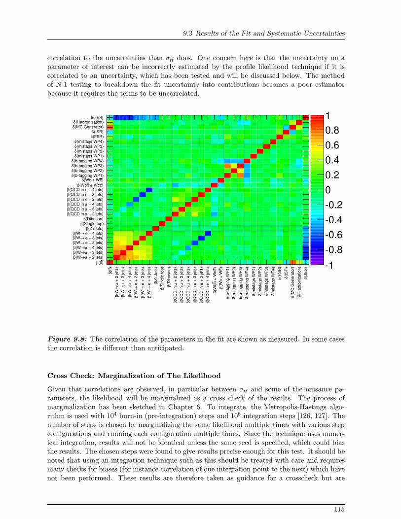
9.3 Results of the Fit and Systematic Uncertainties
correlation to the uncertainties than σtt does. One concern here is that the uncertainty on aparameter of interest can be incorrectly estimated by the profile likelihood technique if it iscorrelated to an uncertainty, which has been tested and will be discussed below. The methodof N-1 testing to breakdown the fit uncertainty into contributions becomes a poor estimatorbecause it requires the terms to be uncorrelated.
1
0.8
0.6
0.4
0.2
0
0.2
0.4
0.6
0.8
1)t
(tβ
+ 2
je
ts)
µ→
(Wβ
+ 3
je
ts)
µ→
(Wβ
+ 4
je
ts)
µ→
(Wβ
e +
2 je
ts)
→(Wβ
e +
3 je
ts)
→(Wβ
e +
4 je
ts)
→(Wβ
(Z+
Je
ts)
β
(Sin
gle
to
p)
β
(Dib
oso
n)
β
+ 2
je
ts)
µ(Q
CD
in
β
+ 3
je
ts)
µ(Q
CD
in
β
+ 4
je
ts)
µ(Q
CD
in
β (Q
CD
in
e +
2 je
ts)
β (QC
D in
e +
3 je
ts)
β (QC
D in
e +
4 je
ts)
β
)c
+ W
cb
(Wb
β
)c
(Wc +
Wβ
(bt
ag
gin
g W
P1
)δ (b
ta
gg
ing
WP
2)
δ (bt
ag
gin
g W
P3
)δ (b
ta
gg
ing
WP
4)
δ
(mis
tag
s W
P1
)δ (m
ista
gs W
P2
)δ (m
ista
gs W
P3
)δ (m
ista
gs W
P4
)δ
(FS
R)
δ
(IS
R)
δ
(MC
Ge
ne
rato
r)δ
(Ha
dro
niz
atio
n)
δ
(JE
S)
δ
)t(tβ + 2 jets)µ→(Wβ + 3 jets)µ→(Wβ + 4 jets)µ→(Wβ
e + 2 jets)→(Wβ e + 3 jets)→(Wβ e + 4 jets)→(Wβ
(Z+Jets)β(Single top)β
(Diboson)β + 2 jets)µ(QCD in β + 3 jets)µ(QCD in β + 4 jets)µ(QCD in β
(QCD in e + 2 jets)β(QCD in e + 3 jets)β(QCD in e + 4 jets)β
)c + Wcb(Wbβ)c(Wc + Wβ
(btagging WP1)δ(btagging WP2)δ(btagging WP3)δ(btagging WP4)δ
(mistags WP1)δ(mistags WP2)δ(mistags WP3)δ(mistags WP4)δ
(FSR)δ(ISR)δ
(MC Generator)δ(Hadronization)δ
(JES)δ
Figure 9.8: The correlation of the parameters in the fit are shown as measured. In some casesthe correlation is different than anticipated.
Cross Check: Marginalization of The Likelihood
Given that correlations are observed, in particular between σtt and some of the nuisance pa-rameters, the likelihood will be marginalized as a cross check of the results. The process ofmarginalization has been sketched in Chapter 6. To integrate, the Metropolis-Hastings algo-rithm is used with 104 burn-in (pre-integration) steps and 106 integration steps [126, 127]. Thenumber of steps is chosen by marginalizing the same likelihood multiple times with various stepconfigurations and running each configuration multiple times. Since the technique uses numer-ical integration, results will not be identical unless the same seed is specified, which could biasthe results. The chosen steps were found to give results precise enough for this test. It should benoted that using an integration technique such as this should be treated with care and requiresmany checks for biases (for instance correlation of one integration point to the next) which havenot been performed. These results are therefore taken as guidance for a crosscheck but are
115

9 Simultaneous Measurement of σtt, fWHF, and fWc in
∫
L dt = 0.7 fb−1
themselves not thoroughly vetted.
Using marginalization, the result for σtt reveals a 2.9 % shift in the central value, with similarbut slightly smaller uncertainty (9.7 % vs. 9.3 %). It is no surprise that the central value shiftsgiven the relatively large correlations measured in data, and it is encouraging that the relativeuncertainty is similar. It would seem reasonable to quote an additional 2.9 % methodologicaluncertainty on the measurement of σtt using the current configuration. Doing so would raisethe “fit” uncertainty from 9.7 % to 10.1 %.
Turning to the heavy flavor cross section, fWHFhas a near identical central value
(∆fWHF=+0.005 %) from profiling and marginalization, while the uncertainty goes up by a
relative 1.1 % (from 18.2 % to 18.4 %). This is considered to be consistent. The case of fWc
is harder to evaluate given both the limited sensitivity of the fit to its contribution and thepreviously discussed issue of low MC statistics. The central value shifts up by 9.2 % whilethe uncertainty stays nearly the same, going down from 24.6 % to 24.2 %. For a method assensitive as marginalization, results for such a problematic parameter should be taken lightlybefore extensive testing is undertaken.
The results of the check with marginalization is shown in Table 9.2, compared with resultsfrom profiling and, in the σtt case, those corrected for the linearity offset. The results of thischeck yield clear evidence that results in a highly-correlated environment with a profile likelihoodfit need to be carefully evaluated. In the case at hand, the difference in the central value forthe results between the marginalized and profiled likelihood could be taken as an additionalmethodological uncertainty. The large uncertainties coming from the rest of the analysis renderthe results practically the same. Accordingly, it would prove more fruitful to study the likelihoodbehavior in such an environment than to simply assign a larger systematic uncertainty.
Method Mean Uncertainty (rel) Median
σtt
Profiling 1.0499 9.7 % -Marginalization 1.0803 9.3 % 1.0766Change (rel) +2.9 % -4.3 % -
Profiling (Uncorrected) 1.0499 9.7 % -Profiling (Linearity Offset) 1.0589 9.7 % -Change (rel) +0.9 % - -
fWHF
Profiling 0.9709 18.2 % -Marginalization 0.9754 18.4 % 0.9756Change (rel) +0.005 % +1.1 % -
fWc
Profiling 0.7377 24.6 % -Marginalization 0.8015 24.2 % 0.7915Change (rel) +9.2 % -1.6 % -
Table 9.2: The results of the marginalized likelihood compared to the profiled likelihood.For each parameter of interest, the results of both are shown. The corrected value for σtt
with profiling is the result after calibrating for the offset observed in the linearity test. Themarginalized uncertainty is the RMS of the mean of the fit, while for profiling it is an averageof the two asymmetric uncertainties (the last two columns in Table 9.1).
116

9.3 Results of the Fit and Systematic Uncertainties
Systematic Uncertainties
The fit uncertainty is broken into components, but for σtt, this breakdown is not reliable dueto large correlations observed. It is nonetheless relatively clear that the generator uncertaintyis dominant, having an uncertainty on its own similar to the rest of the fit combined. Amongstthe externally evaluated systematic uncertainties, electron scale factors, the pileup componentof JES, and the b-JES are dominant, where the lattermost is highly asymmetric. The results aresummarized in Table 9.3. A complete list of sytematic uncertainties considered can be found inAppendix A.
The fWHFfit uncertainty is dominated by the statistical component (13 %), while the domi-
nant object uncertainty in the fit is the b-tagging algorithm calibration. Amongst the externalsystematics, the pileup component of JES dominates along with electron scale factors, where thelatter yields a large asymmetry. It is of note that the MC statistical uncertainty is at the level ofabout 6%. This alone is not a limiting factor but it is likely that not having enough simulationMC statistics artificially enlarges the effects of systematic uncertainties, which thereby obtain astatistical component. The results are summarized in Table 9.3.
The fit uncertainty for fWc is split in almost equal parts between statistical uncertainty andthe b-tagging algorithm calibration, each at the level of about 15 %. Other in-fit uncertaintiesare much smaller. The out of fit uncertainties blow up to large values, often asymmetric. Theworst offender is the pileup JES term, which has a relative uncertainty of +12 - 38 %. This canbe due in part to the insensitivity of the fit to fWc but certainly a large part is due to the low MCstatistics, which alone contributes a 10 % uncertainty. With such an unsmooth and statisticallylimited distribution, evaluation of systematic uncertainties is of limited reliability. The resultsare summarized in Table 9.3.
It should be noted that several commonly considered systematic uncertainties are not takeninto account here. The uncertainty due to PDF is not considered due to purely technicalreasons, but it can be estimated to be of the same order as in the analyses in the previouschapters, about 1%, although it may be large effect on fWHF
. The uncertainty due to modelingof fake leptons is not taken into account. Doing so properly would require a detailed study ofthe flavor composition of such events, which is beyond the scope of this work. The effect shouldbe very small nonetheless: the shape is expected to be similar to the full W+jets shape itself,and therefore most of the events will be in the background dominated first bin. If the analysisin Chapter 7 which used a flavor-sensitive variable as a discriminating variable is any guide,uncertainties should be on the order of 1% due to modeling. Most importantly, the modelinguncertainty of W+jets has not been properly taken into account here. Naively evaluating thesystematic uncertainty using the method described in Chapter 5 yields uncertainties of < 1% onall three parameters. Given that the derivation of the rescaling functions did not take flavor intoaccount it is not obvious that they are readily applicable. Furthermore, the clear dependence ofσtt on the modeling of tt implies that there should be a larger dependence of fWHF
and fWc ontheir MC modeling as well. A more thorough evaluation would use an alternative MC generatorfor W+jets as is done for tt, but no second sample of generated events was available at the time.Additional uncertainties regarding the flavor composition of the backgrounds, in particular ofthe Z+jets sample would be sensible, though the rate is so low it is not likely to be a largeuncertainty.
117

9 Simultaneous Measurement of σtt, fWHF, and fWc in
∫
L dt = 0.7 fb−1
Final Results
The final results of the fit, with all uncertainties taken into account, are
σtt = 172.8 ± 2.8 (stat.)+21−27 (syst.) ± 6.4 (lumi.)pb = 172.8+22
−28 pb,
fWHF= 0.97 ± 0.14 (stat.)+0.21
−0.22 (syst.) ± 0.04 (lumi.) = 0.97+0.25−0.27,
fWc = 0.74 ± 0.16 (stat.)+0.40−0.67 (syst.) ± 0.04 (lumi.) = 0.74+0.45
−0.71.
The results for fWHFand fWc are in clear agreement with the previous measurements from
ATLAS, fWHF= fWc = 1.0. The central value for fWHF
is very close, with comparable uncer-tainty. The fWc measurement is clearly lower, however the uncertainties here are large andwithin those, consistent. The result for σtt will be discussed in the next chapter along with theresults from the other analyses presented in this thesis.
Uncertainty up (pb) down (pb) up (%) down (%)Fit 16.92 −16.80 9.82 −9.76BreakdownStatistical 2.76 −2.76 1.77 −1.77Tag 9.60 −9.46 5.83 −5.75ISR/FSR 8.54 −5.29 5.19 −3.21JES 7.52 −10.42 4.57 −6.33Hadronization 9.09 −8.35 5.52 −5.07Generator 14.21 −13.73 8.63 −8.34ExternalJET/Emiss
T10.92 −19.02 6.64 −11.55
Lepton 8.63 −11.79 5.24 −7.16Template statistics 1.05 −1.05 0.64 −0.64Syst 21.16 −27.40 12.86 −16.65Stat. + Syst 21.39 −27.56 13.00 −16.74Lumi 6.37 −6.37 3.70 −3.70all 22.24 −27.56 13.51 −16.75
Table 9.3: Table of estimated systematic uncertainties for σtt. The breakdown is not reliablebecause of large correlations amongst the parameters. Uncertainty is dominated by the choiceof generator, but the magnitude of its dominance is unclear.
118

9.3 Results of the Fit and Systematic Uncertainties
Uncertainty up (frac) down (frac) up (%) down (%)Fit 0.18 −0.18 18.32 −18.15BreakdownStatistical 0.14 −0.14 13.23 −13.23Tag 0.06 −0.06 5.85 −6.45ISR/FSR 0.04 −0.05 4.23 −5.17JES 0.00 −0.04 0.00 −4.08Hadronization 0.00 −0.04 0.00 −3.70Generator 0.03 −0.04 2.94 −4.50ExternalJET/Emiss
T0.15 −0.13 14.87 −13.42
Lepton 0.05 −0.14 4.72 −13.69Template statistics 0.06 −0.06 6.15 −6.15Syst 0.21 −0.22 20.51 −21.70Stat. + Syst 0.25 −0.26 24.90 −26.41Lumi 0.04 −0.04 3.70 −3.70all 0.25 −0.27 25.17 −26.67
Table 9.4: Table of estimated systematic uncertainties for fWHF. The fit is dominated by statis-
tical error while the overall uncertainty also has major contributions from the pileup componentof JES and the electron scale factor.
Uncertainty up (frac) down (frac) up (%) down (%)Fit 0.19 −0.18 25.2 −23.9BreakdownStatistical 0.16 −0.16 21.6 −21.6Tag 0.13 −0.11 17.6 −14.8ISR/FSR 0.02 −0.02 2.7 −2.7JES 0.06 −0.07 8.1 −9.5Hadronization 0.06 −0.04 8.1 −5.4Generator 0.03 −0.03 4.1 −4.1ExternalJET/Emiss
T0.19 −0.53 25.7 −71.6
Lepton 0.29 −0.41 39.2 −55.4Template statistics 0.10 −0.10 13.5 −13.5Syst 0.40 −0.67 54.1 −90.5Stat. + Syst 0.45 −0.71 60.8 −95.9Lumi 0.04 −0.04 5.4 −5.4all 0.45 −0.71 61.1 −96.1
Table 9.5: Table of estimated systematic uncertainties for fWc. The fit is dominated by thestatistical component with a major contribution from the calibration of the b-tagging algorithm.The pileup JES term and electron scale factor are large and asymmetric. The contribution fromtemplate statistics uncertainty becomes large. This has the effect that externally evaluateduncertainties will be artificially enlarged.
119


10 Interpretations of Results and a Glance
Towards the Future
Three separate measurements of the top quark pair production cross section have been pre-sented in this thesis, each using a binned profile likelihood template fit to data. The firstmeasurement used a likelihood discriminant as input, formed of 3 kinematic variables and theoutput of a b-tagging algorithm, in
∫
L dt= 35 pb−1 of data recorded during 2010. This resultis now submitted for publication, greatly improving the sensitivity of σtt with respect to theprevious ATLAS publication. The second analysis used a similar technique but without explicitflavor sensitivity using
∫
L dt = 0.7 fb−1 of data collected during the first half of 2011. Thethird analysis used a single-variable input to simultaneously measure σtt, fWHF
, and fWc in the∫
L dt = 0.7 fb−1 dataset.The measurements of σtt from the three analyses presented are
σtt = 187 ± 11 (stat.) +18−17 (syst.) ± 6 (lumi.) pb = 187 +22
−21 pb,∫
L dt= 35 pb−1,
σtt = 179 ± 3.9 (stat.) ± 9.0 (syst.) ± 6.6 (lumi.) pb = 179 ± 11.8 pb,∫
L dt = 0.7 fb−1,Ch. 8,
σtt = 173 ± 2.8 (stat.) +21−27 (syst.) ± 6.4 (lumi.) pb = 173 +22
−28 pb,∫
L dt = 0.7 fb−1Ch. 9.
The theoretical prediction used for comparison throughout is
σtt = 164.6+11.5−15.8 pb.
All three measurements of σtt are in agreement with the prediction within uncertainty but aresystematically above the predicted central value by 5-10 %. This can be clearly seen in Fig-ure 10.1, which shows the measurements presented here together with the earlier measurementfrom the collaboration, compared with the prediction. The two most precise measurements usea similar method to each other on different data sets with different observables. The two arestatistically independent and dominated by different systematic uncertainties.
In addition to the top pair production cross section, the analysis in Chapter 9 measuredsimultaneously fWHF
and fWc. These are measured to be
fWHF= 0.97 ± 0.14 (stat.)+0.21
−0.22 (syst.) ± 0.04 (lumi.) pb = 0.97+0.25−0.27,
fWc = 0.74 ± 0.16 (stat.)+0.40−0.67 (syst.) ± 0.04 (lumi.) pb = 0.74+0.45
−0.71.
with respect to the fractions present in the MC simulation scaled to the previous ATLAS mea-surement in the same dataset. The measurement of fWHF
is consistent with the earlier ATLASmeasurement (fWHF
=1), which has different main systematic uncertainties. The uncertainty onfWc in this method is too large to make a meaningful qualitative statement.
The measurement of fWHFis of particular interest here as it measures an important physical
quantity with increased sensitivity with respect to the previous measurement. The ATLASmeasurement which is taken as a starting point was fWHF
= 1.63 ± 0.76 (47 % relative) withrespect to the MC. That measurement was consistent with leading order predictions in the MC
121

10 Interpretations of Results and a Glance Towards the Future
(for which fWHF=1.0 there). Scaling the result of the analysis in Chapter 9 with respect to
the MC yields fWHF= 1.58+41
−44, more clearly above the LO MC than previous measurements.Given that there are relatively large uncertainties for both W+jets in general and heavy-flavorrelated processes in particular, this is not surprising. The results are certainly consistent withintheoretical errors, estimated to be 50-100 %. The same game can be played with fWc. TheATLAS measurement is fWc = 1.11± 0.35 (32 % relative), though here the dedicated ATLASmeasurement is naturally more sensitive, as the analysis variable at hand is not optimizedfor c-jet separation. The measurement of fWHF
supports the earlier findings of ATLAS. Thisestablishes treating the heavy flavor component of W+jets, an irreducible background to tt, asa signal itself in the same measurement using the ATLAS detector.
1
ATLAS 3pb, Ch.7
1
ATLAS 35pb, Ch.8
1
ATLAS 0.7fb, Ch.9
10.7fb
Top P
air
Pro
du
ctio
n C
ross S
ection
100
120
140
160
180
200
220
Theory
Measurements
=172.5 GeV)top
=7 TeV, ms( tt
σ
Figure 10.1: The three measurements presented in this thesis using∫
L dt = 35 pb−1–0.7 fb−1of data, along with the earlier ATLAS measurement using
∫
L dt = 3 pb−1(left mostpoint)[5], and a theoretical prediction (horizontal line, uncertainty band) [13]. Experimentalerror on the most precise σtt determination is smaller than uncertainty of the prediction. Errorbars on measurements include all uncertainties. Both the predictions and measurements assumemtop = 172.5 GeV.
10.1 The Meaning of These Results
The results in this thesis represent the path towards a precision measurement of σtt at ATLAS.The analysis in Chapter 8 using
∫
L dt = 0.7 fb−1 achieves a relative precision of about 7 %,similar to that achieved recently at the Tevatron [71, 72]. It is possible after one year of collidingbeams operation to reach a precision which required a decade at the Tevatron. This is onlynatural given higher statistics, more advanced detector technology, and experience gained inearlier experiments applicable here. Unlike those analyses performed at the Tevatron, which are
122
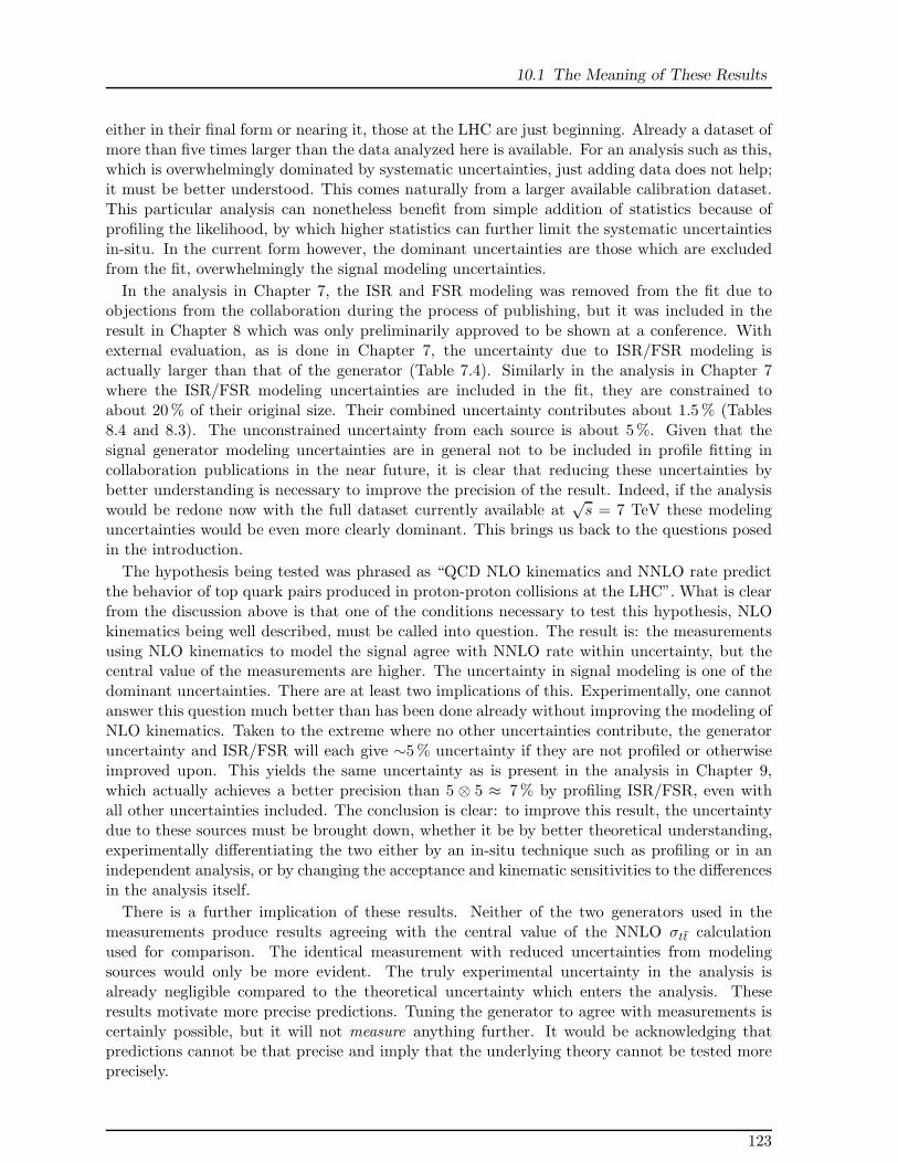
10.1 The Meaning of These Results
either in their final form or nearing it, those at the LHC are just beginning. Already a dataset ofmore than five times larger than the data analyzed here is available. For an analysis such as this,which is overwhelmingly dominated by systematic uncertainties, just adding data does not help;it must be better understood. This comes naturally from a larger available calibration dataset.This particular analysis can nonetheless benefit from simple addition of statistics because ofprofiling the likelihood, by which higher statistics can further limit the systematic uncertaintiesin-situ. In the current form however, the dominant uncertainties are those which are excludedfrom the fit, overwhelmingly the signal modeling uncertainties.
In the analysis in Chapter 7, the ISR and FSR modeling was removed from the fit due toobjections from the collaboration during the process of publishing, but it was included in theresult in Chapter 8 which was only preliminarily approved to be shown at a conference. Withexternal evaluation, as is done in Chapter 7, the uncertainty due to ISR/FSR modeling isactually larger than that of the generator (Table 7.4). Similarly in the analysis in Chapter 7where the ISR/FSR modeling uncertainties are included in the fit, they are constrained toabout 20 % of their original size. Their combined uncertainty contributes about 1.5 % (Tables8.4 and 8.3). The unconstrained uncertainty from each source is about 5%. Given that thesignal generator modeling uncertainties are in general not to be included in profile fitting incollaboration publications in the near future, it is clear that reducing these uncertainties bybetter understanding is necessary to improve the precision of the result. Indeed, if the analysiswould be redone now with the full dataset currently available at
√s = 7 TeV these modeling
uncertainties would be even more clearly dominant. This brings us back to the questions posedin the introduction.
The hypothesis being tested was phrased as “QCD NLO kinematics and NNLO rate predictthe behavior of top quark pairs produced in proton-proton collisions at the LHC”. What is clearfrom the discussion above is that one of the conditions necessary to test this hypothesis, NLOkinematics being well described, must be called into question. The result is: the measurementsusing NLO kinematics to model the signal agree with NNLO rate within uncertainty, but thecentral value of the measurements are higher. The uncertainty in signal modeling is one of thedominant uncertainties. There are at least two implications of this. Experimentally, one cannotanswer this question much better than has been done already without improving the modeling ofNLO kinematics. Taken to the extreme where no other uncertainties contribute, the generatoruncertainty and ISR/FSR will each give ∼5 % uncertainty if they are not profiled or otherwiseimproved upon. This yields the same uncertainty as is present in the analysis in Chapter 9,which actually achieves a better precision than 5 ⊗ 5 ≈ 7% by profiling ISR/FSR, even withall other uncertainties included. The conclusion is clear: to improve this result, the uncertaintydue to these sources must be brought down, whether it be by better theoretical understanding,experimentally differentiating the two either by an in-situ technique such as profiling or in anindependent analysis, or by changing the acceptance and kinematic sensitivities to the differencesin the analysis itself.
There is a further implication of these results. Neither of the two generators used in themeasurements produce results agreeing with the central value of the NNLO σtt calculationused for comparison. The identical measurement with reduced uncertainties from modelingsources would only be more evident. The truly experimental uncertainty in the analysis isalready negligible compared to the theoretical uncertainty which enters the analysis. Theseresults motivate more precise predictions. Tuning the generator to agree with measurements iscertainly possible, but it will not measure anything further. It would be acknowledging thatpredictions cannot be that precise and imply that the underlying theory cannot be tested moreprecisely.
123

10 Interpretations of Results and a Glance Towards the Future
There are a few possibilities in order to better understand the difference between expectationand measurement. It could very well be that the NLO kinematics are not good enough, thathigher-order effects affect the kinematics. One could think of either a full-blown higher ordergenerator or a kinematically dependent k-factor to make the NLO MC behave like a higher orderprediction. On the experimental side, one could think to reduce sensitivity to theoretical uncer-tainty, in particular those due to acceptance. Broadening kinematic cuts would reduce sensitivityto kinematic differences between generators, however this would greatly increase experimentaluncertainties, those affecting jets in particular. Another possibility would be unfolding the mea-surement to quote a fiducial cross section. Such projects may be undertaken in the future, andindeed many discussions have begun amongst various physicists along these lines. It is clearthat simply rerunning these analyses without first making progress on these issues will not leadto a deeper knowledge of nature.
10.2 An Outlook: The Coming Precision
The measurements presented here, in particular those using the∫
L dt = 0.7 fb−1 dataset, hailthe arrival of the era of precision physics above the scale of the W and Z bosons. The topquark is now being studied to extreme precision, not only in the inclusive production crosssection measurement described here. In recent months, results have become available such asthe production cross section of top quark pairs with an additional photon and with additionaljets [129, 130], as well as inclusive production in the difficult all-hadronic decay channel [131].Differential cross section measurements have been made, analyzing effects such as the chargeasymmetry in top quark pair production at the LHC [132]. Measurements of single-top quarkproduction cross section have been made as well [133]. Properties of the top quark are beingmeasured, in particular the mass and charge [134, 135]. Most of these measurements are ap-proaching the precision of similar measurements at the Tevatron and will soon surpass them, ifthey have not already. These measurements test and verify properties and behavior of the topquark.
Such knowledge allows for searches for particles and interactions which are not a part of theStandard Model, and for setting limits on many theories which could exist over a very broadenergy range. Knowledge of the top quark was used, for instance, in a search for particles whichdecay into a tt pair, attempting to measuring an excess of tt events [136]. Indeed analysesthroughout the collaboration are setting limits on such theories not only using top quarks. Thisis done in particular setting lower limits for the masses of particles based on the non-observationof them. Many theories, some popular, are becoming disfavored as a result. To date thereis no direct evidence for particles or interactions which are not already understood within theStandard Model.
The Standard Model is being tested to high precision in many ways. The inclusive crosssection of rare processes such as di-boson production have been recently measured and foundto be in agreement with NLO QCD predictions [137, 138, 139]. Here, as in the case of thetop quark pair production cross section, it may soon become necessary to obtain more precisepredictions in order to test QCD at a higher order. Those analyses are statistically limited asof yet, with systematic uncertainties of a similar magnitude as the predictions. One of the lastpredictions of the SM which is not verified is the production of a Higgs boson, being searchedfor vigorously by all collaborations in the field. Stringent limits have recently been set by boththe ATLAS and CMS collaborations, effectively ruling out the possibility of a SM Higgs over ahuge mass range [37, 38]. Only a small range remains, in which there is some insignificant but
124
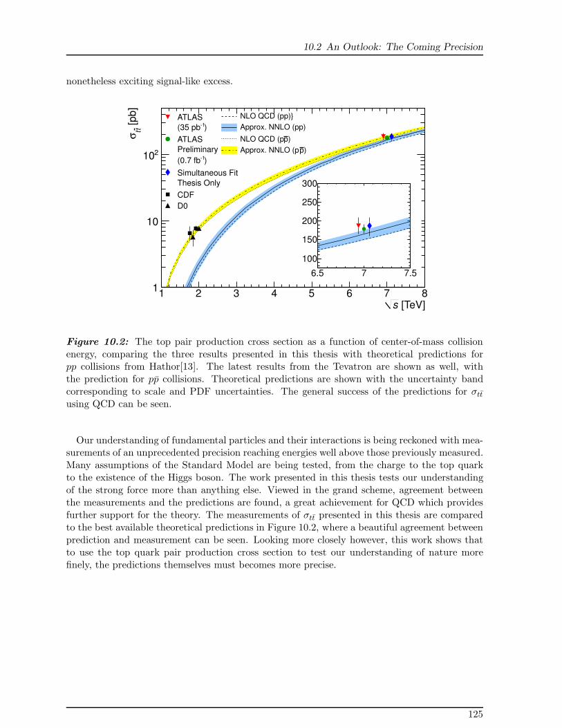
10.2 An Outlook: The Coming Precision
nonetheless exciting signal-like excess.
[TeV]s1 2 3 4 5 6 7 8
[p
b]
t tσ
1
10
210
ATLAS
)1(35 pb
ATLAS
Preliminary
)1(0.7 fb
Simultaneous Fit
Thesis Only
CDF
D0
NLO QCD (pp)}
Approx. NNLO (pp)
)pNLO QCD (p
)pApprox. NNLO (p
6.5 7 7.5
100
150
200
250
300
Figure 10.2: The top pair production cross section as a function of center-of-mass collisionenergy, comparing the three results presented in this thesis with theoretical predictions forpp collisions from Hathor[13]. The latest results from the Tevatron are shown as well, withthe prediction for pp collisions. Theoretical predictions are shown with the uncertainty bandcorresponding to scale and PDF uncertainties. The general success of the predictions for σtt
using QCD can be seen.
Our understanding of fundamental particles and their interactions is being reckoned with mea-surements of an unprecedented precision reaching energies well above those previously measured.Many assumptions of the Standard Model are being tested, from the charge to the top quarkto the existence of the Higgs boson. The work presented in this thesis tests our understandingof the strong force more than anything else. Viewed in the grand scheme, agreement betweenthe measurements and the predictions are found, a great achievement for QCD which providesfurther support for the theory. The measurements of σtt presented in this thesis are comparedto the best available theoretical predictions in Figure 10.2, where a beautiful agreement betweenprediction and measurement can be seen. Looking more closely however, this work shows thatto use the top quark pair production cross section to test our understanding of nature morefinely, the predictions themselves must becomes more precise.
125


A Summary of Systematic Uncertainties
The detector related systematic uncertainties considered in the analyses are summarized here.
• JES Jet Energy Scale, nine components in total: Calo, Eta, Noise, Flavor, b-JES, Alpgen,Perugia, Close-by, Pileup.
• JER Jet Energy Resolution.
• JRE Jet Reconstruction Efficiency.
• JRE Jet Reconstruction Efficiency.
• ESS Electron Energy Scale
• ESR Electron Energy Resolution
• ESF Electron Scale Factors, 3 components: trigger, reconstruction, identification.
• MMS Muon Momentum Scale.
• MSS Muon Momentum Resolution, considered separately for ID and MS for∫
L dt = 0.7 fb−1.
• MSF Muon Scale Factors, 3 components: trigger, reconstruction, identification.
• MET Missing Energy Resolution, soft jet and cell out terms.
• LAr LAr calorimeter gap, only∫
L dt = 0.7 fb−1.
• b-Tag Calibration of the b-tagging algorithm efficiency.
• mistag Calibration of the b-tagging algorithm mistagging rate.
In addition, contributions due to modeling of the signal are considered:
• Generator Considering POWHEG as signal in place of MC@NLO.
• Hadronization Considering PYTHIA for the parton shower of the signal simulation inplace of HERWIG.
• ISR Initial State Radiation, increased and decreased from nominal.
• FSR Final State Radiation, increased and decreased from nominal.
• PDF Vary within envelope of PDF set uncertainty.
Modeling variations of the dominant sources of background to the signal are considered as well.Uncertainty on the rate of background processes are used directly as input to the measurement.Alternate models considered are:
• W Shape Generation parameters in ALPGEN varied.
127

A Summary of Systematic Uncertainties
• QCD Shape Alternate estimation from data using different method or control region.
In addition, two methodological uncertainties are considered:
• Lumi Luminosity normalization.
• Template Statistics Statistical uncertainty of MC Simulation.
128

B Kinematic Comparison of tt in MC@NLO
and POWHEG
The basic kinematic expectations of the tt signal process generated by MC@NLO are comparedto the identical distributions in POWHEG. In the analyses here, MC@NLO is used for thesignal model and POWHEG is used as an alternative to assess systematic uncertainties. Thesamples are generated, simulated, and reconstructed as described in Chapter 4 of this thesis. Alldistributions are shown in the e+jets channel after object selection at the reconstruction levelwith no truth-matching applied. The simulation shown corresponds to the
∫
L dt = 0.7 fb−1
dataset, for which a total of 15 million events were generated using MC@NLO and 3 millionusing POWHEG. The only error shown is statistical. The fact that limited statistics are availableprobably causes the estimated size of the systematic uncertainty due to this in the analyses inthis thesis to be overestimated.
The pT and η of both jets and the electrons are compared. The missing energy and transversemass of the W boson are shown as well. The distribution of the CombNNJetFitter b-taggingalgorithm for the most b-like jet is also shown. All comparisons use the 3-jet bin, the 4-jet bin,and the 5-jet inclusive bin, organized in jet multiplicities. All distributions are normalized tounity, shown for each distribution both overlayed and divided (MC@NLO/POWHEG).
The most interesting feature of these comparisons is seen in the leading jet pT when lookingat the three jet bins, shown side by side in Figure B.1. In the 3-jet bin the POWHEG simulationshows a softer spectrum than that of MC@NLO while in the 5-jet bin the trend is evidentlyreversed and POWHEG is harder. In the 4-jet bin the distributions are quite similar for theleading jet pT. The effect is clearest in the 5-jet bin, where the trend can be seen for each jet inthe event.
TLeading Jet P
40 60 80 100 120 140 160 180 200 220
Norm
aliz
ed, A
rbitra
ry U
nits
0
0.02
0.04
0.06
0.08
0.1
0.12 MC@NLO
POWHEG
TLeading Jet P
40 60 80 100 120 140 160 180 200 220
MC@NLO/POWHEG
0.8
0.9
1
1.1
1.2
1.3
TLeading Jet P
40 60 80 100 120 140 160 180 200 220
Norm
aliz
ed, A
rbitra
ry U
nits
0
0.02
0.04
0.06
0.08
0.1
0.12
0.14
0.16
MC@NLO
POWHEG
TLeading Jet P
40 60 80 100 120 140 160 180 200 220
MC@NLO/POWHEG
0.8
0.85
0.9
0.95
1
1.05
1.1
1.15
1.2
TLeading Jet P
50 100 150 200 250 300
Norm
aliz
ed, A
rbitra
ry U
nits
0
0.02
0.04
0.06
0.08
0.1
MC@NLO
POWHEG
TLeading Jet P
50 100 150 200 250 300
MC@NLO/POWHEG
0.75
0.8
0.85
0.9
0.95
1
1.05
1.1
1.15
1.2
Figure B.1: Kinematic comparison of the leading jet pT in MC@NLO and POWHEG in thee+jets channel. The left most plot is the 3-jet bin, followed by the 4-jet bin and the 5-jetinclsuive bin.
129

B Kinematic Comparison of tt in MC@NLO and POWHEG
TLeading Jet P
40 60 80 100 120 140 160 180 200 220
Norm
aliz
ed, A
rbitra
ry U
nits
0
0.02
0.04
0.06
0.08
0.1
0.12 MC@NLO
POWHEG
TLeading Jet P
40 60 80 100 120 140 160 180 200 220
MC@NLO/POWHEG
0.8
0.9
1
1.1
1.2
1.3
TSecond Jet P
40 60 80 100 120 140 160 180 200 220
Norm
aliz
ed, A
rbitra
ry U
nits
0
0.02
0.04
0.06
0.08
0.1
0.12
0.14
0.16
0.18
0.2
MC@NLO
POWHEG
TSecond Jet P
40 60 80 100 120 140 160 180 200 220
MC@NLO/POWHEG
1
1.1
1.2
1.3
1.4
TThird Jet P
30 40 50 60 70 80 90 100 110 120
Norm
aliz
ed, A
rbitra
ry U
nits
0
0.05
0.1
0.15
0.2
0.25MC@NLO
POWHEG
TThird Jet P
30 40 50 60 70 80 90 100 110 120
MC@NLO/POWHEG
0.8
0.9
1
1.1
1.2
1.3
1.4
ηLeading Jet 2.5 2 1.5 1 0.5 0 0.5 1 1.5 2 2.5
Norm
aliz
ed, A
rbitra
ry U
nits
0.02
0.04
0.06
0.08
0.1 MC@NLO
POWHEG
ηLeading Jet 2.5 2 1.5 1 0.5 0 0.5 1 1.5 2 2.5
MC@NLO/POWHEG
0.8
0.85
0.9
0.95
1
1.05
1.1
1.15
1.2
ηSecond Jet 2.5 2 1.5 1 0.5 0 0.5 1 1.5 2 2.5
Norm
aliz
ed, A
rbitra
ry U
nits
0.02
0.03
0.04
0.05
0.06
0.07
0.08
0.09
0.1
MC@NLO
POWHEG
ηSecond Jet 2.5 2 1.5 1 0.5 0 0.5 1 1.5 2 2.5
MC@NLO/POWHEG
0.8
0.85
0.9
0.95
1
1.05
1.1
1.15
1.2
ηThird Jet 2.5 2 1.5 1 0.5 0 0.5 1 1.5 2 2.5
Norm
aliz
ed, A
rbitra
ry U
nits
0.02
0.03
0.04
0.05
0.06
0.07
0.08
0.09MC@NLO
POWHEG
ηThird Jet 2.5 2 1.5 1 0.5 0 0.5 1 1.5 2 2.5
MC@NLO/POWHEG
0.8
0.85
0.9
0.95
1
1.05
1.1
1.15
1.2
, most blike jetω4 2 0 2 4 6 8
Norm
aliz
ed, A
rbitra
ry U
nits
0
0.02
0.04
0.06
0.08
0.1 MC@NLO
POWHEG
, most blike jetω4 2 0 2 4 6 8
MC@NLO/POWHEG
0.8
0.85
0.9
0.95
1
1.05
1.1
1.15
1.2
TElectron P
30 40 50 60 70 80 90 100 110 120
Norm
aliz
ed, A
rbitra
ry U
nits
0.02
0.04
0.06
0.08
0.1
0.12MC@NLO
POWHEG
TElectron P
30 40 50 60 70 80 90 100 110 120
MC@NLO/POWHEG
0.8
0.85
0.9
0.95
1
1.05
1.1
1.15
1.2
ηElectron 2.5 2 1.5 1 0.5 0 0.5 1 1.5 2 2.5
Norm
aliz
ed, A
rbitra
ry U
nits
0.02
0.04
0.06
0.08
0.1
0.12
MC@NLO
POWHEG
ηElectron 2.5 2 1.5 1 0.5 0 0.5 1 1.5 2 2.5
MC@NLO/POWHEG
0.8
0.85
0.9
0.95
1
1.05
1.1
1.15
1.2
missing
TE40 60 80 100 120 140 160 180 200 220
Norm
aliz
ed, A
rbitra
ry U
nits
0
0.02
0.04
0.06
0.08
0.1
0.12
0.14
0.16 MC@NLO
POWHEG
missing
TE
40 60 80 100 120 140 160 180 200 220
MC@NLO/POWHEG
0.9
1
1.1
1.2
1.3
1.4
W Transverse Mass40 60 80 100 120 140 160 180 200 220
Norm
aliz
ed, A
rbitra
ry U
nits
0
0.02
0.04
0.06
0.08
0.1
0.12
0.14
0.16
MC@NLO
POWHEG
W Transverse Mass40 60 80 100 120 140 160 180 200 220
MC@NLO/POWHEG
0.8
0.85
0.9
0.95
1
1.05
1.1
1.15
1.2
Figure B.2: Kinematic comparison of MC@NLO and POWHEG in the e+3 jets bin.
130

TLeading Jet P
40 60 80 100 120 140 160 180 200 220
Norm
aliz
ed, A
rbitra
ry U
nits
0
0.02
0.04
0.06
0.08
0.1
0.12
0.14
0.16
MC@NLO
POWHEG
TLeading Jet P
40 60 80 100 120 140 160 180 200 220
MC@NLO/POWHEG
0.8
0.85
0.9
0.95
1
1.05
1.1
1.15
1.2
TSecond Jet P
40 60 80 100 120 140 160 180 200 220
Norm
aliz
ed, A
rbitra
ry U
nits
0
0.02
0.04
0.06
0.08
0.1
0.12
0.14
0.16
0.18
0.2
0.22
0.24
MC@NLO
POWHEG
TSecond Jet P
40 60 80 100 120 140 160 180 200 220
MC@NLO/POWHEG
0.8
0.85
0.9
0.95
1
1.05
1.1
1.15
1.2
TThird Jet P
40 60 80 100 120 140 160 180 200 220
Norm
aliz
ed, A
rbitra
ry U
nits
0
0.05
0.1
0.15
0.2
0.25
0.3
0.35
MC@NLO
POWHEG
TThird Jet P
40 60 80 100 120 140 160 180 200 220
MC@NLO/POWHEG
0.8
0.85
0.9
0.95
1
1.05
1.1
1.15
1.2
TFourth Jet P
40 60 80 100 120 140 160 180 200 220
Norm
aliz
ed, A
rbitra
ry U
nits
0
0.1
0.2
0.3
0.4
0.5
0.6
0.7 MC@NLO
POWHEG
TFourth Jet P
40 60 80 100 120 140 160 180 200 220
MC@NLO/POWHEG
0.8
0.85
0.9
0.95
1
1.05
1.1
1.15
1.2
ηLeading Jet 2.5 2 1.5 1 0.5 0 0.5 1 1.5 2 2.5
Norm
aliz
ed, A
rbitra
ry U
nits
0.02
0.04
0.06
0.08
0.1 MC@NLO
POWHEG
ηLeading Jet 2.5 2 1.5 1 0.5 0 0.5 1 1.5 2 2.5
MC@NLO/POWHEG
0.8
0.85
0.9
0.95
1
1.05
1.1
1.15
1.2
ηSecond Jet 2.5 2 1.5 1 0.5 0 0.5 1 1.5 2 2.5
Norm
aliz
ed, A
rbitra
ry U
nits
0.02
0.04
0.06
0.08
0.1MC@NLO
POWHEG
ηSecond Jet 2.5 2 1.5 1 0.5 0 0.5 1 1.5 2 2.5
MC@NLO/POWHEG
0.8
0.85
0.9
0.95
1
1.05
1.1
1.15
1.2
ηThird Jet 2.5 2 1.5 1 0.5 0 0.5 1 1.5 2 2.5
Norm
aliz
ed, A
rbitra
ry U
nits
0.02
0.03
0.04
0.05
0.06
0.07
0.08
0.09
0.1
MC@NLO
POWHEG
ηThird Jet 2.5 2 1.5 1 0.5 0 0.5 1 1.5 2 2.5
MC@NLO/POWHEG
0.8
0.85
0.9
0.95
1
1.05
1.1
1.15
1.2
ηFourth Jet 2.5 2 1.5 1 0.5 0 0.5 1 1.5 2 2.5
Norm
aliz
ed, A
rbitra
ry U
nits
0.02
0.03
0.04
0.05
0.06
0.07
0.08
0.09
MC@NLO
POWHEG
ηFourth Jet 2.5 2 1.5 1 0.5 0 0.5 1 1.5 2 2.5
MC@NLO/POWHEG
0.8
0.85
0.9
0.95
1
1.05
1.1
1.15
1.2
, most blike jetω4 2 0 2 4 6 8
Norm
aliz
ed, A
rbitra
ry U
nits
0
0.02
0.04
0.06
0.08
0.1
0.12MC@NLO
POWHEG
, most blike jetω4 2 0 2 4 6 8
MC@NLO/POWHEG
0.8
0.85
0.9
0.95
1
1.05
1.1
1.15
1.2
TElectron P
40 60 80 100 120 140 160 180 200 220
Norm
aliz
ed, A
rbitra
ry U
nits
0
0.02
0.04
0.06
0.08
0.1
0.12
0.14
0.16
0.18
0.2
0.22
0.24
MC@NLO
POWHEG
TElectron P
40 60 80 100 120 140 160 180 200 220
MC@NLO/POWHEG
0.8
0.85
0.9
0.95
1
1.05
1.1
1.15
1.2
ηElectron 2.5 2 1.5 1 0.5 0 0.5 1 1.5 2 2.5
Norm
aliz
ed, A
rbitra
ry U
nits
0.02
0.04
0.06
0.08
0.1
0.12
MC@NLO
POWHEG
ηElectron 2.5 2 1.5 1 0.5 0 0.5 1 1.5 2 2.5
MC@NLO/POWHEG
0.8
0.85
0.9
0.95
1
1.05
1.1
1.15
1.2
missing
TE40 60 80 100 120 140 160 180 200 220
Norm
aliz
ed, A
rbitra
ry U
nits
0
0.02
0.04
0.06
0.08
0.1
0.12
0.14
0.16
0.18
MC@NLO
POWHEG
missing
TE
40 60 80 100 120 140 160 180 200 220
MC@NLO/POWHEG
0.8
0.85
0.9
0.95
1
1.05
1.1
1.15
1.2
W Transverse Mass40 60 80 100 120 140 160 180 200 220
Norm
aliz
ed, A
rbitra
ry U
nits
0
0.02
0.04
0.06
0.08
0.1
0.12
0.14
0.16
0.18
MC@NLO
POWHEG
W Transverse Mass40 60 80 100 120 140 160 180 200 220
MC@NLO/POWHEG
0.8
0.85
0.9
0.95
1
1.05
1.1
1.15
1.2
Figure B.3: Kinematic comparison of MC@NLO and POWHEG in the e+4 jets bin.
131

B Kinematic Comparison of tt in MC@NLO and POWHEG
TLeading Jet P
50 100 150 200 250 300
Norm
aliz
ed, A
rbitra
ry U
nits
0
0.02
0.04
0.06
0.08
0.1
MC@NLO
POWHEG
TLeading Jet P
50 100 150 200 250 300
MC@NLO/POWHEG
0.75
0.8
0.85
0.9
0.95
1
1.05
1.1
1.15
1.2
TSecond Jet P
50 100 150 200 250 300
Norm
aliz
ed, A
rbitra
ry U
nits
0
0.02
0.04
0.06
0.08
0.1
0.12
0.14
0.16
MC@NLO
POWHEG
TSecond Jet P
50 100 150 200 250 300
MC@NLO/POWHEG
0.5
0.6
0.7
0.8
0.9
1
1.1
1.2
1.3
TThird Jet P
30 40 50 60 70 80 90 100 110 120
Norm
aliz
ed, A
rbitra
ry U
nits
0
0.02
0.04
0.06
0.08
0.1
0.12
MC@NLO
POWHEG
TThird Jet P
30 40 50 60 70 80 90 100 110 120
MC@NLO/POWHEG
0.8
0.85
0.9
0.95
1
1.05
1.1
1.15
1.2
TFourth Jet P
30 40 50 60 70 80 90 100 110 120
Norm
aliz
ed, A
rbitra
ry U
nits
0
0.02
0.04
0.06
0.08
0.1
0.12
0.14
0.16 MC@NLO
POWHEG
TFourth Jet P
30 40 50 60 70 80 90 100 110 120
MC@NLO/POWHEG
0.7
0.8
0.9
1
1.1
ηLeading Jet 2.5 2 1.5 1 0.5 0 0.5 1 1.5 2 2.5
Norm
aliz
ed, A
rbitra
ry U
nits
0.02
0.04
0.06
0.08
0.1 MC@NLO
POWHEG
ηLeading Jet 2.5 2 1.5 1 0.5 0 0.5 1 1.5 2 2.5
MC@NLO/POWHEG
0.8
0.85
0.9
0.95
1
1.05
1.1
1.15
1.2
ηSecond Jet 2.5 2 1.5 1 0.5 0 0.5 1 1.5 2 2.5
Norm
aliz
ed, A
rbitra
ry U
nits
0.02
0.04
0.06
0.08
0.1 MC@NLO
POWHEG
ηSecond Jet 2.5 2 1.5 1 0.5 0 0.5 1 1.5 2 2.5
MC@NLO/POWHEG
0.8
0.85
0.9
0.95
1
1.05
1.1
1.15
1.2
ηThird Jet 2.5 2 1.5 1 0.5 0 0.5 1 1.5 2 2.5
Norm
aliz
ed, A
rbitra
ry U
nits
0.02
0.03
0.04
0.05
0.06
0.07
0.08
0.09
0.1
MC@NLO
POWHEG
ηThird Jet 2.5 2 1.5 1 0.5 0 0.5 1 1.5 2 2.5
MC@NLO/POWHEG
0.8
0.85
0.9
0.95
1
1.05
1.1
1.15
1.2
ηFourth Jet 2.5 2 1.5 1 0.5 0 0.5 1 1.5 2 2.5
Norm
aliz
ed, A
rbitra
ry U
nits
0.02
0.03
0.04
0.05
0.06
0.07
0.08
0.09MC@NLO
POWHEG
ηFourth Jet 2.5 2 1.5 1 0.5 0 0.5 1 1.5 2 2.5
MC@NLO/POWHEG
0.8
0.85
0.9
0.95
1
1.05
1.1
1.15
1.2
, most blike jetω4 2 0 2 4 6 8
Norm
aliz
ed, A
rbitra
ry U
nits
0
0.02
0.04
0.06
0.08
0.1
0.12 MC@NLO
POWHEG
, most blike jetω4 2 0 2 4 6 8
MC@NLO/POWHEG
0.8
0.85
0.9
0.95
1
1.05
1.1
1.15
1.2
TElectron P
30 40 50 60 70 80 90 100 110 120
Norm
aliz
ed, A
rbitra
ry U
nits
0.02
0.04
0.06
0.08
0.1
0.12
MC@NLO
POWHEG
TElectron P
30 40 50 60 70 80 90 100 110 120
MC@NLO/POWHEG
0.9
0.95
1
1.05
1.1
1.15
1.2
1.25
ηElectron 2.5 2 1.5 1 0.5 0 0.5 1 1.5 2 2.5
Norm
aliz
ed, A
rbitra
ry U
nits
0
0.02
0.04
0.06
0.08
0.1
0.12
MC@NLO
POWHEG
ηElectron 2.5 2 1.5 1 0.5 0 0.5 1 1.5 2 2.5
MC@NLO/POWHEG
0.8
0.85
0.9
0.95
1
1.05
1.1
1.15
1.2
missing
TE40 60 80 100 120 140 160 180 200 220
Norm
aliz
ed, A
rbitra
ry U
nits
0
0.02
0.04
0.06
0.08
0.1
0.12
0.14
0.16MC@NLO
POWHEG
missing
TE
40 60 80 100 120 140 160 180 200 220
MC@NLO/POWHEG
0.8
0.85
0.9
0.95
1
1.05
1.1
1.15
1.2
W Transverse Mass40 60 80 100 120 140 160 180 200 220
Norm
aliz
ed, A
rbitra
ry U
nits
0
0.02
0.04
0.06
0.08
0.1
0.12
0.14
0.16MC@NLO
POWHEG
W Transverse Mass40 60 80 100 120 140 160 180 200 220
MC@NLO/POWHEG
0.8
0.85
0.9
0.95
1
1.05
1.1
1.15
1.2
Figure B.4: Kinematic comparison of MC@NLO and POWHEG in the e+5 jets (inclusive)bin.
132

C Control Plots for the∫
L dt = 35 pb−1
Dataset
The expectations from MC simulation compared with observed data for the∫
L dt= 35 pb−1
dataset. All plots are shown for each jet multiplicity available, including the 4-jet bin, bothinclusive and exclusive. The 5-jet bin is always inclusive. The e+jets channel is shown.
133

C Control Plots for the∫
L dt= 35 pb−1 Dataset
(j1)[GeV]T
p0 50 100 150 200 250 300 350 400
En
trie
s/1
0.0
0
0
500
1000
1500
2000
2500
3000
3500
4000
4500 s = 7 TeV√data
ttW+JetsQCDZsingle top
diboson
1 L dt = 35 pb∫
e+jets
(j1)[GeV]T
p0 50 100 150 200 250 300 350 400
En
trie
s/1
0.0
0
0
100
200
300
400
500
600
700 s = 7 TeV√data
ttW+JetsQCDZsingle top
diboson
1 L dt = 35 pb∫
e + 2 Jets
(j1)[GeV]T
p0 50 100 150 200 250 300 350 400
En
trie
s/1
0.0
0
0
20
40
60
80
100
120
140 s = 7 TeV√data
ttW+JetsQCDZsingle top
diboson
1 L dt = 35 pb∫
e + 3 Jets
(j1)[GeV]T
p0 50 100 150 200 250 300 350 400
En
trie
s/1
0.0
0
0
5
10
15
20
25
30
35
40
45 s = 7 TeV√data tt
W+JetsQCDZsingle top
diboson
1 L dt = 35 pb∫
e + 4 Jets
(j1)[GeV]T
p0 50 100 150 200 250 300 350 400
En
trie
s/1
0.0
0
0
10
20
30
40
50
60
70 s = 7 TeV√data tt
W+JetsQCDZsingle top
diboson
1 L dt = 35 pb∫
4 Jets≥e +
(j1)[GeV]T
p0 50 100 150 200 250 300 350 400
En
trie
s/1
0.0
0
0
5
10
15
20
25
30 s = 7 TeV√data
ttW+JetsQCDZsingle top
diboson
1 L dt = 35 pb∫
5 Jets≥e +
Figure C.1: Leading jet pT in the e+jets channel.
134

(j1)η5 4 3 2 1 0 1 2 3 4 5
En
trie
s/0
.40
0
200
400
600
800
1000
1200
1400
1600 s = 7 TeV√data
ttW+JetsQCDZsingle top
diboson
1 L dt = 35 pb∫
e+jets
(j1)η5 4 3 2 1 0 1 2 3 4 5
En
trie
s/0
.40
0
50
100
150
200
250
300
350
400
450 s = 7 TeV√data tt
W+JetsQCDZsingle top
diboson
1 L dt = 35 pb∫
e + 2 Jets
(j1)η5 4 3 2 1 0 1 2 3 4 5
En
trie
s/0
.40
0
20
40
60
80
100
120
140 s = 7 TeV√data tt
W+JetsQCDZsingle top
diboson
1 L dt = 35 pb∫
e + 3 Jets
(j1)η5 4 3 2 1 0 1 2 3 4 5
En
trie
s/0
.40
0
10
20
30
40
50
60
70 s = 7 TeV√data
ttW+JetsQCDZsingle top
diboson
1 L dt = 35 pb∫
e + 4 Jets
(j1)η5 4 3 2 1 0 1 2 3 4 5
En
trie
s/0
.40
0
10
20
30
40
50
60
70
80
90 s = 7 TeV√data
ttW+JetsQCDZsingle top
diboson
1 L dt = 35 pb∫
4 Jets≥e +
(j1)η5 4 3 2 1 0 1 2 3 4 5
En
trie
s/0
.40
0
5
10
15
20
25
30 s = 7 TeV√data
ttW+JetsQCDZsingle top
diboson
1 L dt = 35 pb∫
5 Jets≥e +
Figure C.2: Leading jet η in the e+jets channel.
135

C Control Plots for the∫
L dt= 35 pb−1 Dataset
(e)[GeV]T
p0 20 40 60 80 100 120 140 160 180 200
En
trie
s/5
.00
0
500
1000
1500
2000
2500
3000 s = 7 TeV√data
ttW+JetsQCDZsingle top
diboson
1 L dt = 35 pb∫
e+jets
(e)[GeV]T
p0 20 40 60 80 100 120 140 160 180 200
En
trie
s/5
.00
0
100
200
300
400
500
600 s = 7 TeV√data
ttW+JetsQCDZsingle top
diboson
1 L dt = 35 pb∫
e + 2 Jets
(e)[GeV]T
p0 20 40 60 80 100 120 140 160 180 200
En
trie
s/5
.00
0
20
40
60
80
100
120
140
160
180 s = 7 TeV√data tt
W+JetsQCDZsingle top
diboson
1 L dt = 35 pb∫
e + 3 Jets
(e)[GeV]T
p0 20 40 60 80 100 120 140 160 180 200
En
trie
s/5
.00
0
10
20
30
40
50
60
70 s = 7 TeV√data
ttW+JetsQCDZsingle top
diboson
1 L dt = 35 pb∫
e + 4 Jets
(e)[GeV]T
p0 20 40 60 80 100 120 140 160 180 200
En
trie
s/5
.00
0
10
20
30
40
50
60
70
80
90 s = 7 TeV√data
ttW+JetsQCDZsingle top
diboson
1 L dt = 35 pb∫
4 Jets≥e +
(e)[GeV]T
p0 20 40 60 80 100 120 140 160 180 200
En
trie
s/5
.00
0
5
10
15
20
25
30 s = 7 TeV√data
ttW+JetsQCDZsingle top
diboson
1 L dt = 35 pb∫
5 Jets≥e +
Figure C.3: Electron pT.
136
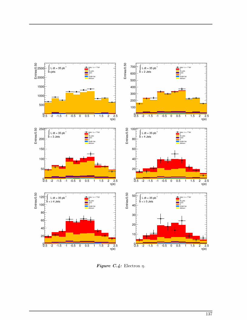
(e)η2.5 2 1.5 1 0.5 0 0.5 1 1.5 2 2.5
En
trie
s/0
.50
0
500
1000
1500
2000
2500 s = 7 TeV√data tt
W+JetsQCDZsingle top
diboson
1 L dt = 35 pb∫
e+jets
(e)η2.5 2 1.5 1 0.5 0 0.5 1 1.5 2 2.5
En
trie
s/0
.50
0
100
200
300
400
500
600
700 s = 7 TeV√data tt
W+JetsQCDZsingle top
diboson
1 L dt = 35 pb∫
e + 2 Jets
(e)η2.5 2 1.5 1 0.5 0 0.5 1 1.5 2 2.5
En
trie
s/0
.50
0
50
100
150
200
250 s = 7 TeV√data
ttW+JetsQCDZsingle top
diboson
1 L dt = 35 pb∫
e + 3 Jets
(e)η2.5 2 1.5 1 0.5 0 0.5 1 1.5 2 2.5
En
trie
s/0
.50
0
20
40
60
80
100 s = 7 TeV√data
ttW+JetsQCDZsingle top
diboson
1 L dt = 35 pb∫
e + 4 Jets
(e)η2.5 2 1.5 1 0.5 0 0.5 1 1.5 2 2.5
En
trie
s/0
.50
0
20
40
60
80
100
120 s = 7 TeV√data tt
W+JetsQCDZsingle top
diboson
1 L dt = 35 pb∫
4 Jets≥e +
(e)η2.5 2 1.5 1 0.5 0 0.5 1 1.5 2 2.5
En
trie
s/0
.50
0
10
20
30
40
50 s = 7 TeV√data
ttW+JetsQCDZsingle top
diboson
1 L dt = 35 pb∫
5 Jets≥e +
Figure C.4: Electron η.
137

C Control Plots for the∫
L dt= 35 pb−1 Dataset
[GeV]TE0 20 40 60 80 100 120 140 160 180 200
En
trie
s/5
.00
0
500
1000
1500
2000
2500
3000 s = 7 TeV√data
ttW+JetsQCDZsingle top
diboson
1 L dt = 35 pb∫
e+jets
[GeV]TE0 20 40 60 80 100 120 140 160 180 200
En
trie
s/5
.00
0
100
200
300
400
500
600
700
800 s = 7 TeV√data tt
W+JetsQCDZsingle top
diboson
1 L dt = 35 pb∫
e + 2 Jets
[GeV]TE0 20 40 60 80 100 120 140 160 180 200
En
trie
s/5
.00
0
20
40
60
80
100
120
140
160
180
200 s = 7 TeV√data
ttW+JetsQCDZsingle top
diboson
1 L dt = 35 pb∫
e + 3 Jets
[GeV]TE0 20 40 60 80 100 120 140 160 180 200
En
trie
s/5
.00
0
10
20
30
40
50 s = 7 TeV√data
ttW+JetsQCDZsingle top
diboson
1 L dt = 35 pb∫
e + 4 Jets
[GeV]TE0 20 40 60 80 100 120 140 160 180 200
En
trie
s/5
.00
0
10
20
30
40
50
60
70 s = 7 TeV√data
ttW+JetsQCDZsingle top
diboson
1 L dt = 35 pb∫
4 Jets≥e +
[GeV]TE0 20 40 60 80 100 120 140 160 180 200
En
trie
s/5
.00
0
5
10
15
20
25 s = 7 TeV√data
ttW+JetsQCDZsingle top
diboson
1 L dt = 35 pb∫
5 Jets≥e +
Figure C.5: EmissT in the e+jets channel.
138
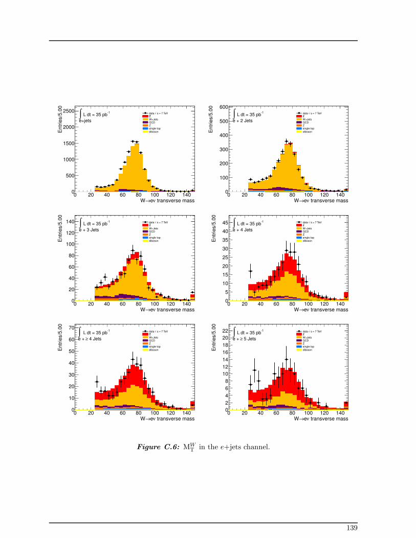
transverse massνe→W0 20 40 60 80 100 120 140
En
trie
s/5
.00
0
500
1000
1500
2000
2500 s = 7 TeV√data
ttW+JetsQCDZsingle top
diboson
1 L dt = 35 pb∫
e+jets
transverse massνe→W0 20 40 60 80 100 120 140
En
trie
s/5
.00
0
100
200
300
400
500
600 s = 7 TeV√data
ttW+JetsQCDZsingle top
diboson
1 L dt = 35 pb∫
e + 2 Jets
transverse massνe→W0 20 40 60 80 100 120 140
En
trie
s/5
.00
0
20
40
60
80
100
120
140 s = 7 TeV√data tt
W+JetsQCDZsingle top
diboson
1 L dt = 35 pb∫
e + 3 Jets
transverse massνe→W0 20 40 60 80 100 120 140
En
trie
s/5
.00
0
5
10
15
20
25
30
35
40
45 s = 7 TeV√data tt
W+JetsQCDZsingle top
diboson
1 L dt = 35 pb∫
e + 4 Jets
transverse massνe→W0 20 40 60 80 100 120 140
En
trie
s/5
.00
0
10
20
30
40
50
60
70 s = 7 TeV√data
ttW+JetsQCDZsingle top
diboson
1 L dt = 35 pb∫
4 Jets≥e +
transverse massνe→W0 20 40 60 80 100 120 140
En
trie
s/5
.00
0
2
4
6
8
10
12
14
16
18
20
22 s = 7 TeV√data tt
W+JetsQCDZsingle top
diboson
1 L dt = 35 pb∫
5 Jets≥e +
Figure C.6: MWT in the e+jets channel.
139


D Control Plots for the∫
L dt = 0.7 fb−1
Dataset
The expectations from MC simulation compared with observed data for the∫
L dt = 0.7 fb−1
dataset. All plots are shown for each jet multiplicity available, including the 4-jet bin, bothinclusive and exclusive. The 5-jet bin is always inclusive. Both the e+jets channel and µ+jetschannel are shown.
141

D Control Plots for the∫
L dt = 0.7 fb−1 Dataset
(leading jet) [GeV]T
p0 50 100 150 200 250 300 350 400
Eve
nts
/ 1
0 G
eV
0
10000
20000
30000
40000
50000
60000
70000
80000 = 7 TeVsData 2011,
tt
W+Jets
QCD Multijet
Z+Jets
Single Top
Diboson
1 L dt = 0.7 fb∫
e+ 1 Jet
(leading jet) [GeV]T
p0 50 100 150 200 250 300 350 400
Eve
nts
/ 1
0 G
eV
0
2000
4000
6000
8000
10000
12000
14000
16000 = 7 TeVsData 2011,
tt
W+Jets
QCD Multijet
Z+Jets
Single Top
Diboson
1 L dt = 0.7 fb∫
e+ 2 Jets
(leading jet) [GeV]T
p0 50 100 150 200 250 300 350 400
Eve
nts
/ 1
0 G
eV
0
500
1000
1500
2000
2500
3000
= 7 TeVsData 2011,
tt
W+Jets
QCD Multijet
Z+Jets
Single Top
Diboson
1 L dt = 0.7 fb∫
e+ 3 Jets
(leading jet) [GeV]T
p0 50 100 150 200 250 300 350 400
Eve
nts
/ 1
0 G
eV
0
100
200
300
400
500
600
700
800
900
= 7 TeVsData 2011,
tt
W+Jets
QCD Multijet
Z+Jets
Single Top
Diboson
1 L dt = 0.7 fb∫
e+ 4 Jets
(leading jet) [GeV]T
p0 50 100 150 200 250 300 350 400
Eve
nts
/ 1
0 G
eV
0
200
400
600
800
1000
1200 = 7 TeVsData 2011,
tt
W+Jets
QCD Multijet
Z+Jets
Single Top
Diboson
1 L dt = 0.7 fb∫
4 Jets≥e+
(leading jet) [GeV]T
p0 50 100 150 200 250 300 350 400
Eve
nts
/ 1
0 G
eV
0
50
100
150
200
250
300
350
400
450 = 7 TeVsData 2011,
tt
W+Jets
QCD Multijet
Z+Jets
Single Top
Diboson
1 L dt = 0.7 fb∫
5 Jets≥e+
Figure D.1: Leading jet pT in the e+jets channel.
142

(leading jet)η2.5 2 1.5 1 0.5 0 0.5 1 1.5 2 2.5
Eve
nts
/ 0
.50
0
5000
10000
15000
20000
25000
30000
35000 = 7 TeVsData 2011,
tt
W+Jets
QCD Multijet
Z+Jets
Single Top
Diboson
1 L dt = 0.7 fb∫
e+ 1 Jet
(leading jet)η2.5 2 1.5 1 0.5 0 0.5 1 1.5 2 2.5
Eve
nts
/ 0
.50
0
2000
4000
6000
8000
10000 = 7 TeVsData 2011,
tt
W+Jets
QCD Multijet
Z+Jets
Single Top
Diboson
1 L dt = 0.7 fb∫
e+ 2 Jets
(leading jet)η2.5 2 1.5 1 0.5 0 0.5 1 1.5 2 2.5
Eve
nts
/ 0
.50
0
500
1000
1500
2000
2500
3000 = 7 TeVsData 2011,
tt
W+Jets
QCD Multijet
Z+Jets
Single Top
Diboson
1 L dt = 0.7 fb∫
e+ 3 Jets
(leading jet)η2.5 2 1.5 1 0.5 0 0.5 1 1.5 2 2.5
Eve
nts
/ 0
.50
0
200
400
600
800
1000
1200 = 7 TeVsData 2011,
tt
W+Jets
QCD Multijet
Z+Jets
Single Top
Diboson
1 L dt = 0.7 fb∫
e+ 4 Jets
(leading jet)η2.5 2 1.5 1 0.5 0 0.5 1 1.5 2 2.5
Eve
nts
/ 0
.50
0
500
1000
1500
2000
2500
= 7 TeVsData 2011,
tt
W+Jets
QCD Multijet
Z+Jets
Single Top
Diboson
1 L dt = 0.7 fb∫
4 Jets≥e+
(leading jet)η2.5 2 1.5 1 0.5 0 0.5 1 1.5 2 2.5
Eve
nts
/ 0
.50
0
100
200
300
400
500
600
700
800
900 = 7 TeVsData 2011,
tt
W+Jets
QCD Multijet
Z+Jets
Single Top
Diboson
1 L dt = 0.7 fb∫
5 Jets≥e+
Figure D.2: Leading jet η in the e+jets channel.
143
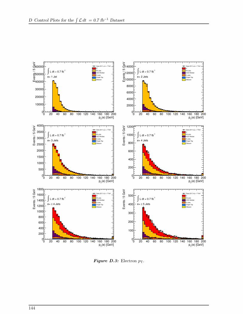
D Control Plots for the∫
L dt = 0.7 fb−1 Dataset
(e) [GeV]T
p0 20 40 60 80 100 120 140 160 180 200
Eve
nts
/ 5
Ge
V
0
10000
20000
30000
40000
50000
60000 = 7 TeVsData 2011,
tt
W+Jets
QCD Multijet
Z+Jets
Single Top
Diboson
1 L dt = 0.7 fb∫
e+ 1 Jet
(e) [GeV]T
p0 20 40 60 80 100 120 140 160 180 200
Eve
nts
/ 5
Ge
V
0
2000
4000
6000
8000
10000
12000
14000 = 7 TeVsData 2011,
tt
W+Jets
QCD Multijet
Z+Jets
Single Top
Diboson
1 L dt = 0.7 fb∫
e+ 2 Jets
(e) [GeV]T
p0 20 40 60 80 100 120 140 160 180 200
Eve
nts
/ 5
Ge
V
0
500
1000
1500
2000
2500
3000
3500
4000
= 7 TeVsData 2011,
tt
W+Jets
QCD Multijet
Z+Jets
Single Top
Diboson
1 L dt = 0.7 fb∫
e+ 3 Jets
(e) [GeV]T
p0 20 40 60 80 100 120 140 160 180 200
Eve
nts
/ 5
Ge
V
0
200
400
600
800
1000
1200 = 7 TeVsData 2011,
tt
W+Jets
QCD Multijet
Z+Jets
Single Top
Diboson
1 L dt = 0.7 fb∫
e+ 4 Jets
(e) [GeV]T
p0 20 40 60 80 100 120 140 160 180 200
Eve
nts
/ 5
Ge
V
0
200
400
600
800
1000
1200
1400
1600
1800
= 7 TeVsData 2011,
tt
W+Jets
QCD Multijet
Z+Jets
Single Top
Diboson
1 L dt = 0.7 fb∫
4 Jets≥e+
(e) [GeV]T
p0 20 40 60 80 100 120 140 160 180 200
Eve
nts
/ 5
Ge
V
0
100
200
300
400
500 = 7 TeVsData 2011,
tt
W+Jets
QCD Multijet
Z+Jets
Single Top
Diboson
1 L dt = 0.7 fb∫
5 Jets≥e+
Figure D.3: Electron pT.
144

(e)η2.5 2 1.5 1 0.5 0 0.5 1 1.5 2 2.5
Eve
nts
/ 0
.25
0
2000
4000
6000
8000
10000
12000
14000
16000
18000 = 7 TeVsData 2011,
tt
W+Jets
QCD Multijet
Z+Jets
Single Top
Diboson
1 L dt = 0.7 fb∫
e+ 1 Jet
(e)η2.5 2 1.5 1 0.5 0 0.5 1 1.5 2 2.5
Eve
nts
/ 0
.25
0
1000
2000
3000
4000
5000 = 7 TeVsData 2011,
tt
W+Jets
QCD Multijet
Z+Jets
Single Top
Diboson
1 L dt = 0.7 fb∫
e+ 2 Jets
(e)η2.5 2 1.5 1 0.5 0 0.5 1 1.5 2 2.5
Eve
nts
/ 0
.25
0
200
400
600
800
1000
1200
1400
1600
1800 = 7 TeVsData 2011,
tt
W+Jets
QCD Multijet
Z+Jets
Single Top
Diboson
1 L dt = 0.7 fb∫
e+ 3 Jets
(e)η2.5 2 1.5 1 0.5 0 0.5 1 1.5 2 2.5
Eve
nts
/ 0
.25
0
100
200
300
400
500
600 = 7 TeVsData 2011,
tt
W+Jets
QCD Multijet
Z+Jets
Single Top
Diboson
1 L dt = 0.7 fb∫
e+ 4 Jets
(e)η2.5 2 1.5 1 0.5 0 0.5 1 1.5 2 2.5
Eve
nts
/ 0
.25
0
200
400
600
800
1000
1200 = 7 TeVsData 2011,
tt
W+Jets
QCD Multijet
Z+Jets
Single Top
Diboson
1 L dt = 0.7 fb∫
4 Jets≥e+
(e)η2.5 2 1.5 1 0.5 0 0.5 1 1.5 2 2.5
Eve
nts
/ 0
.25
0
50
100
150
200
250
300
350
400
450 = 7 TeVsData 2011,
tt
W+Jets
QCD Multijet
Z+Jets
Single Top
Diboson
1 L dt = 0.7 fb∫
5 Jets≥e+
Figure D.4: Electron η.
145

D Control Plots for the∫
L dt = 0.7 fb−1 Dataset
[GeV]TE
0 20 40 60 80 100 120 140 160 180 200
Eve
nts
/ 5
0
10000
20000
30000
40000
50000
60000 = 7 TeVsData 2011,
tt
W+Jets
QCD Multijet
Z+Jets
Single Top
Diboson
1 L dt = 0.7 fb∫
e+ 1 Jet
[GeV]TE
0 20 40 60 80 100 120 140 160 180 200
Eve
nts
/ 5
0
2000
4000
6000
8000
10000
12000
14000
16000 = 7 TeVsData 2011,
tt
W+Jets
QCD Multijet
Z+Jets
Single Top
Diboson
1 L dt = 0.7 fb∫
e+ 2 Jets
[GeV]TE
0 20 40 60 80 100 120 140 160 180 200
Eve
nts
/ 5
0
500
1000
1500
2000
2500
3000
3500
4000 = 7 TeVsData 2011,
tt
W+Jets
QCD Multijet
Z+Jets
Single Top
Diboson
1 L dt = 0.7 fb∫
e+ 3 Jets
[GeV]TE
0 20 40 60 80 100 120 140 160 180 200
Eve
nts
/ 5
0
200
400
600
800
1000
= 7 TeVsData 2011,
tt
W+Jets
QCD Multijet
Z+Jets
Single Top
Diboson
1 L dt = 0.7 fb∫
e+ 4 Jets
[GeV]TE
0 20 40 60 80 100 120 140 160 180 200
Eve
nts
/ 5
0
200
400
600
800
1000
1200
1400
1600 = 7 TeVsData 2011,
tt
W+Jets
QCD Multijet
Z+Jets
Single Top
Diboson
1 L dt = 0.7 fb∫
4 Jets≥e+
[GeV]TE
0 20 40 60 80 100 120 140 160 180 200
Eve
nts
/ 5
0
50
100
150
200
250
300
350
400
450 = 7 TeVsData 2011,
tt
W+Jets
QCD Multijet
Z+Jets
Single Top
Diboson
1 L dt = 0.7 fb∫
5 Jets≥e+
Figure D.5: EmissT in the e+jets channel.
146

(W) [GeV]Tm
0 20 40 60 80 100 120 140
Eve
nts
/ 5
0
10000
20000
30000
40000
50000 = 7 TeVsData 2011,
tt
W+Jets
QCD Multijet
Z+Jets
Single Top
Diboson
1 L dt = 0.7 fb∫
e+ 1 Jet
(W) [GeV]Tm
0 20 40 60 80 100 120 140
Eve
nts
/ 5
0
2000
4000
6000
8000
10000
12000 = 7 TeVsData 2011,
tt
W+Jets
QCD Multijet
Z+Jets
Single Top
Diboson
1 L dt = 0.7 fb∫
e+ 2 Jets
(W) [GeV]Tm
0 20 40 60 80 100 120 140
Eve
nts
/ 5
0
500
1000
1500
2000
2500 = 7 TeVsData 2011,
tt
W+Jets
QCD Multijet
Z+Jets
Single Top
Diboson
1 L dt = 0.7 fb∫
e+ 3 Jets
(W) [GeV]Tm
0 20 40 60 80 100 120 140
Eve
nts
/ 5
0
100
200
300
400
500
600
700 = 7 TeVsData 2011,
tt
W+Jets
QCD Multijet
Z+Jets
Single Top
Diboson
1 L dt = 0.7 fb∫
e+ 4 Jets
(W) [GeV]Tm
0 20 40 60 80 100 120 140
Eve
nts
/ 5
0
200
400
600
800
1000 = 7 TeVsData 2011,
tt
W+Jets
QCD Multijet
Z+Jets
Single Top
Diboson
1 L dt = 0.7 fb∫
4 Jets≥e+
(W) [GeV]Tm
0 20 40 60 80 100 120 140
Eve
nts
/ 5
0
50
100
150
200
250
300
350 = 7 TeVsData 2011,
tt
W+Jets
QCD Multijet
Z+Jets
Single Top
Diboson
1 L dt = 0.7 fb∫
5 Jets≥e+
Figure D.6: MWT in the e+jets channel.
147

D Control Plots for the∫
L dt = 0.7 fb−1 Dataset
(leading jet) [GeV]T
p0 50 100 150 200 250 300 350 400
Eve
nts
/ 1
0 G
eV
0
20
40
60
80
100
120
140
160
180
200
220
310×
= 7 TeVsData 2011,
tt
W+Jets
QCD Multijet
Z+Jets
Single Top
Diboson
1 L dt = 0.7 fb∫+ 1 Jetµ
(leading jet) [GeV]T
p0 50 100 150 200 250 300 350 400
Eve
nts
/ 1
0 G
eV
0
5000
10000
15000
20000
25000
30000
35000
40000 = 7 TeVsData 2011,
tt
W+Jets
QCD Multijet
Z+Jets
Single Top
Diboson
1 L dt = 0.7 fb∫+ 2 Jetsµ
(leading jet) [GeV]T
p0 50 100 150 200 250 300 350 400
Eve
nts
/ 1
0 G
eV
0
1000
2000
3000
4000
5000
6000 = 7 TeVsData 2011,
tt
W+Jets
QCD Multijet
Z+Jets
Single Top
Diboson
1 L dt = 0.7 fb∫+ 3 Jetsµ
(leading jet) [GeV]T
p0 50 100 150 200 250 300 350 400
Eve
nts
/ 1
0 G
eV
0
200
400
600
800
1000
1200
1400 = 7 TeVsData 2011,
tt
W+Jets
QCD Multijet
Z+Jets
Single Top
Diboson
1 L dt = 0.7 fb∫+ 4 Jetsµ
(leading jet) [GeV]T
p0 50 100 150 200 250 300 350 400
Eve
nts
/ 1
0 G
eV
0
200
400
600
800
1000
1200
1400
1600
1800
2000 = 7 TeVsData 2011,
tt
W+Jets
QCD Multijet
Z+Jets
Single Top
Diboson
1 L dt = 0.7 fb∫
4 Jets≥+ µ
(leading jet) [GeV]T
p0 50 100 150 200 250 300 350 400
Eve
nts
/ 1
0 G
eV
0
100
200
300
400
500
600 = 7 TeVsData 2011,
tt
W+Jets
QCD Multijet
Z+Jets
Single Top
Diboson
1 L dt = 0.7 fb∫
5 Jets≥+ µ
Figure D.7: Leading jet pT in the µ+jets channel.
148
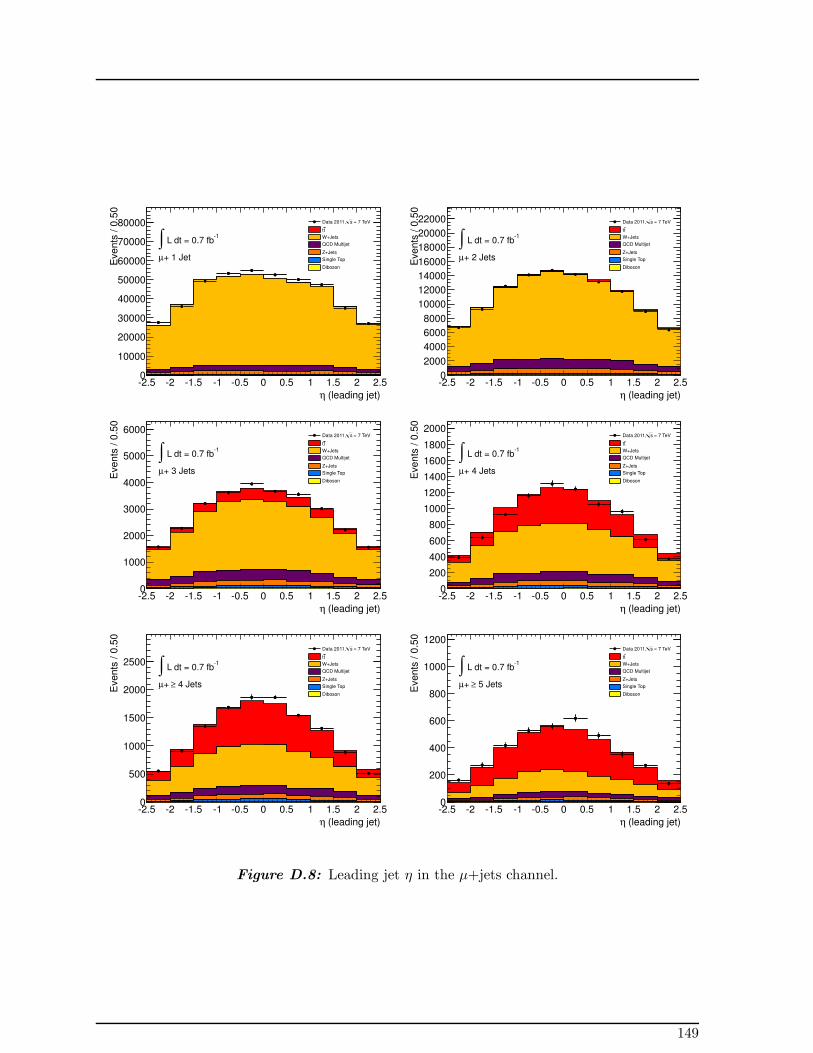
(leading jet)η2.5 2 1.5 1 0.5 0 0.5 1 1.5 2 2.5
Eve
nts
/ 0
.50
0
10000
20000
30000
40000
50000
60000
70000
80000 = 7 TeVsData 2011,
tt
W+Jets
QCD Multijet
Z+Jets
Single Top
Diboson
1 L dt = 0.7 fb∫+ 1 Jetµ
(leading jet)η2.5 2 1.5 1 0.5 0 0.5 1 1.5 2 2.5
Eve
nts
/ 0
.50
0
2000
4000
6000
8000
10000
12000
14000
16000
18000
20000
22000 = 7 TeVsData 2011,
tt
W+Jets
QCD Multijet
Z+Jets
Single Top
Diboson
1 L dt = 0.7 fb∫+ 2 Jetsµ
(leading jet)η2.5 2 1.5 1 0.5 0 0.5 1 1.5 2 2.5
Eve
nts
/ 0
.50
0
1000
2000
3000
4000
5000
6000 = 7 TeVsData 2011,
tt
W+Jets
QCD Multijet
Z+Jets
Single Top
Diboson
1 L dt = 0.7 fb∫+ 3 Jetsµ
(leading jet)η2.5 2 1.5 1 0.5 0 0.5 1 1.5 2 2.5
Eve
nts
/ 0
.50
0
200
400
600
800
1000
1200
1400
1600
1800
2000 = 7 TeVsData 2011,
tt
W+Jets
QCD Multijet
Z+Jets
Single Top
Diboson
1 L dt = 0.7 fb∫+ 4 Jetsµ
(leading jet)η2.5 2 1.5 1 0.5 0 0.5 1 1.5 2 2.5
Eve
nts
/ 0
.50
0
500
1000
1500
2000
2500
= 7 TeVsData 2011,
tt
W+Jets
QCD Multijet
Z+Jets
Single Top
Diboson
1 L dt = 0.7 fb∫
4 Jets≥+ µ
(leading jet)η2.5 2 1.5 1 0.5 0 0.5 1 1.5 2 2.5
Eve
nts
/ 0
.50
0
200
400
600
800
1000
1200 = 7 TeVsData 2011,
tt
W+Jets
QCD Multijet
Z+Jets
Single Top
Diboson
1 L dt = 0.7 fb∫
5 Jets≥+ µ
Figure D.8: Leading jet η in the µ+jets channel.
149

D Control Plots for the∫
L dt = 0.7 fb−1 Dataset
) [GeV]µ(T
p0 20 40 60 80 100 120 140 160 180 200
Eve
nts
/ 5
Ge
V
0
20
40
60
80
100
120310×
= 7 TeVsData 2011,
tt
W+Jets
QCD Multijet
Z+Jets
Single Top
Diboson
1 L dt = 0.7 fb∫+ 1 Jetµ
) [GeV]µ(T
p0 20 40 60 80 100 120 140 160 180 200
Eve
nts
/ 5
Ge
V
0
5000
10000
15000
20000
25000
30000 = 7 TeVsData 2011,
tt
W+Jets
QCD Multijet
Z+Jets
Single Top
Diboson
1 L dt = 0.7 fb∫+ 2 Jetsµ
) [GeV]µ(T
p0 20 40 60 80 100 120 140 160 180 200
Eve
nts
/ 5
Ge
V
0
1000
2000
3000
4000
5000
6000
7000
8000 = 7 TeVsData 2011,
tt
W+Jets
QCD Multijet
Z+Jets
Single Top
Diboson
1 L dt = 0.7 fb∫+ 3 Jetsµ
) [GeV]µ(T
p0 20 40 60 80 100 120 140 160 180 200
Eve
nts
/ 5
Ge
V
0
200
400
600
800
1000
1200
1400
1600
1800
2000
2200 = 7 TeVsData 2011,
tt
W+Jets
QCD Multijet
Z+Jets
Single Top
Diboson
1 L dt = 0.7 fb∫+ 4 Jetsµ
) [GeV]µ(T
p0 20 40 60 80 100 120 140 160 180 200
Eve
nts
/ 5
Ge
V
0
500
1000
1500
2000
2500
3000 = 7 TeVsData 2011,
tt
W+Jets
QCD Multijet
Z+Jets
Single Top
Diboson
1 L dt = 0.7 fb∫
4 Jets≥+ µ
) [GeV]µ(T
p0 20 40 60 80 100 120 140 160 180 200
Eve
nts
/ 5
Ge
V
0
100
200
300
400
500
600
700
800 = 7 TeVsData 2011,
tt
W+Jets
QCD Multijet
Z+Jets
Single Top
Diboson
1 L dt = 0.7 fb∫
5 Jets≥+ µ
Figure D.9: Muon pT.
150

)µ(η2.5 2 1.5 1 0.5 0 0.5 1 1.5 2 2.5
Eve
nts
/ 0
.25
0
5000
10000
15000
20000
25000
30000
35000
40000 = 7 TeVsData 2011,
tt
W+Jets
QCD Multijet
Z+Jets
Single Top
Diboson
1 L dt = 0.7 fb∫+ 1 Jetµ
)µ(η2.5 2 1.5 1 0.5 0 0.5 1 1.5 2 2.5
Eve
nts
/ 0
.25
0
2000
4000
6000
8000
10000
12000
14000
16000 = 7 TeVsData 2011,
tt
W+Jets
QCD Multijet
Z+Jets
Single Top
Diboson
1 L dt = 0.7 fb∫+ 2 Jetsµ
)µ(η2.5 2 1.5 1 0.5 0 0.5 1 1.5 2 2.5
Eve
nts
/ 0
.25
0
500
1000
1500
2000
2500
3000
3500
4000
4500 = 7 TeVsData 2011,
tt
W+Jets
QCD Multijet
Z+Jets
Single Top
Diboson
1 L dt = 0.7 fb∫+ 3 Jetsµ
)µ(η2.5 2 1.5 1 0.5 0 0.5 1 1.5 2 2.5
Eve
nts
/ 0
.25
0
200
400
600
800
1000 = 7 TeVsData 2011,
tt
W+Jets
QCD Multijet
Z+Jets
Single Top
Diboson
1 L dt = 0.7 fb∫+ 4 Jetsµ
)µ(η2.5 2 1.5 1 0.5 0 0.5 1 1.5 2 2.5
Eve
nts
/ 0
.25
0
200
400
600
800
1000
1200
1400
1600 = 7 TeVsData 2011,
tt
W+Jets
QCD Multijet
Z+Jets
Single Top
Diboson
1 L dt = 0.7 fb∫
4 Jets≥+ µ
)µ(η2.5 2 1.5 1 0.5 0 0.5 1 1.5 2 2.5
Eve
nts
/ 0
.25
0
100
200
300
400
500 = 7 TeVsData 2011,
tt
W+Jets
QCD Multijet
Z+Jets
Single Top
Diboson
1 L dt = 0.7 fb∫
5 Jets≥+ µ
Figure D.10: Muon η.
151

D Control Plots for the∫
L dt = 0.7 fb−1 Dataset
[GeV]TE
0 20 40 60 80 100 120 140 160 180 200
Eve
nts
/ 5
0
10000
20000
30000
40000
50000
60000
70000
80000 = 7 TeVsData 2011,
tt
W+Jets
QCD Multijet
Z+Jets
Single Top
Diboson
1 L dt = 0.7 fb∫+ 1 Jetµ
[GeV]TE
0 20 40 60 80 100 120 140 160 180 200
Eve
nts
/ 5
0
2000
4000
6000
8000
10000
12000
14000
16000
18000
20000 = 7 TeVsData 2011,
tt
W+Jets
QCD Multijet
Z+Jets
Single Top
Diboson
1 L dt = 0.7 fb∫+ 2 Jetsµ
[GeV]TE
0 20 40 60 80 100 120 140 160 180 200
Eve
nts
/ 5
0
500
1000
1500
2000
2500
3000
3500
4000
4500 = 7 TeVsData 2011,
tt
W+Jets
QCD Multijet
Z+Jets
Single Top
Diboson
1 L dt = 0.7 fb∫+ 3 Jetsµ
[GeV]TE
0 20 40 60 80 100 120 140 160 180 200
Eve
nts
/ 5
0
200
400
600
800
1000
= 7 TeVsData 2011,
tt
W+Jets
QCD Multijet
Z+Jets
Single Top
Diboson
1 L dt = 0.7 fb∫+ 4 Jetsµ
[GeV]TE
0 20 40 60 80 100 120 140 160 180 200
Eve
nts
/ 5
0
200
400
600
800
1000
1200
1400
1600 = 7 TeVsData 2011,
tt
W+Jets
QCD Multijet
Z+Jets
Single Top
Diboson
1 L dt = 0.7 fb∫
4 Jets≥+ µ
[GeV]TE
0 20 40 60 80 100 120 140 160 180 200
Eve
nts
/ 5
0
50
100
150
200
250
300
350
400
450 = 7 TeVsData 2011,
tt
W+Jets
QCD Multijet
Z+Jets
Single Top
Diboson
1 L dt = 0.7 fb∫
5 Jets≥+ µ
Figure D.11: EmissT in the µ+jets channel.
152

(W) [GeV]Tm
0 20 40 60 80 100 120 140
Eve
nts
/ 5
0
10000
20000
30000
40000
50000
60000
70000
80000 = 7 TeVsData 2011,
tt
W+Jets
QCD Multijet
Z+Jets
Single Top
Diboson
1 L dt = 0.7 fb∫+ 1 Jetµ
(W) [GeV]Tm
0 20 40 60 80 100 120 140
Eve
nts
/ 5
0
2000
4000
6000
8000
10000
12000
14000
16000 = 7 TeVsData 2011,
tt
W+Jets
QCD Multijet
Z+Jets
Single Top
Diboson
1 L dt = 0.7 fb∫+ 2 Jetsµ
(W) [GeV]Tm
0 20 40 60 80 100 120 140
Eve
nts
/ 5
0
1000
2000
3000
4000
5000 = 7 TeVsData 2011,
tt
W+Jets
QCD Multijet
Z+Jets
Single Top
Diboson
1 L dt = 0.7 fb∫+ 3 Jetsµ
(W) [GeV]Tm
0 20 40 60 80 100 120 140
Eve
nts
/ 5
0
200
400
600
800
1000
= 7 TeVsData 2011,
tt
W+Jets
QCD Multijet
Z+Jets
Single Top
Diboson
1 L dt = 0.7 fb∫+ 4 Jetsµ
(W) [GeV]Tm
0 20 40 60 80 100 120 140
Eve
nts
/ 5
0
200
400
600
800
1000
1200
1400
1600 = 7 TeVsData 2011,
tt
W+Jets
QCD Multijet
Z+Jets
Single Top
Diboson
1 L dt = 0.7 fb∫
4 Jets≥+ µ
(W) [GeV]Tm
0 20 40 60 80 100 120 140
Eve
nts
/ 5
0
50
100
150
200
250
300
350
400
450 = 7 TeVsData 2011,
tt
W+Jets
QCD Multijet
Z+Jets
Single Top
Diboson
1 L dt = 0.7 fb∫
5 Jets≥+ µ
Figure D.12: MWT in the µ+jets channel.
153


Citogenesis.“I just read a pop-science book by a respected author. One chapter, and muchof the thesis, was based around wildly inaccurate data which traced back to...Wikipedia. Toencourage people to be on their toes, I’m not going to say what book or author.”[19]

Bibliography
[1] W. Pauli, Pauli letter collection: letter to Lise Meitner, Pauli Archives, CERN.
[2] H. Geiger and E. Marsden, On a Diffuse Reflection of the α-Particles, Proceedings of theRoyal Society of London. Series A 82(557) (1909) 495.
[3] E. Rutherford, The scattering of α and β particles by matter and the structure of theatom, Philosophical Magazine Series 6 21(125) (1911) 669.
[4] R. R. D. Ulam S, von Neumann J, Statistical Methods in Neutron Diffusion, Letter,April 9, 1947. LAMS-551.
[5] The Atlas Collaboration, G. Aad et al., Measurement of the top quark-pair productioncross section with ATLAS in pp collisions at
√s = 7 TeV, Eur.Phys.J. C71 (2011) 1577,
hep-ph/1012.1792.
[6] The CMS Collaboration, V. Khachatryan et al., First Measurement of the Cross Sectionfor Top-Quark Pair Production in Proton-Proton Collisions at
√s = 7 TeV, Phys.Lett.
B695 (2011) 424, hep-ph/1010.5994.
[7] P. Nason and B. Webber, Next-to-Leading-Order Event Generators, hep-ph/1202.1251.
[8] S. Frixione and B. R. Webber, Matching NLO QCD computations and parton showersimulations, JHEP 0206 (2002) 029, hep-ph/0204244.
[9] S. Frixione, P. Nason, and B. R. Webber, Matching NLO QCD and parton showers inheavy flavor production, JHEP 0308 (2003) 007, hep-ph/0305252.
[10] P. Nason, A New method for combining NLO QCD with shower Monte Carlo algorithms,JHEP 0411 (2004) 040, hep-ph/0409146.
[11] S. Hoeche, F. Krauss, M. Schonherr, and F. Siegert, A critical appraisal of NLO+PSmatching methods, hep-ph/1111.1220.
[12] J. M. Campbell, K. R. Ellis, and C. Williams, MCFM: A Monte Carlo for FeMtobarnprocesses at Hadron Colliders, User’s Guide, http://mcfm.fnal.gov/mcfm.pdf.
[13] M. Aliev et al., HATHOR: HAdronic Top and Heavy quarks crOss section calculatoR,Comput.Phys.Commun. 182 (2011) 1034, hep-ph/1007.1327.
[14] V. Ferrara, A. Henrichs, U. Husemann, C. Lange, A. Quadt, A. Roe, E. Shabalina, andH. Zhu, Measurement of the top quark cross-section in the semileptonic channel in ppcollisions at
√s=7 TeV using kinematic fits and b-tagging information,
ATL-COM-PHYS-2011-1012.
[15] V. Ahrens, M. Neubert, B. D. Pecjak, A. Ferroglia, and L. L. Yang, Precision predictionsfor the tt production cross section at hadron colliders, Phys.Lett. B703 (2011) 135,1105.5824.
157
Bibliography
[16] Measurement of the ttbar production cross-section in pp collisions at√s = 7 TeV using
kinematic information of lepton+jets events.
[17] The ATLAS Collaboration, G. Aad et al., Measurement of the top quark pair productioncross-section with ATLAS in the single lepton channel, hep-ex/1201.1889, Submitted toPhys. Lett. B 9 January 2012.
[18] A. D. Roeck, Top Production at Hadron Colliders, XXV International Symposium onLepton Photon Interactions at High Energies. Mumbai, India, 22-27 August 2011.Proceedings not yet published.
[19] XKCD, Comic reprinted from xkcd.com, February 2012.
[20] P. A. M. Dirac, The Quantum Theory of the Electron, Proceedings of the Royal Societyof London. Series A 117(778) (1928) 610.
[21] K. Nakamura and P. D. Group, Review of Particle Physics, Journal of Physics G:Nuclear and Particle Physics (2010) 075021, Updated online in 2011, http://pdg.lbl.gov/.
[22] The Tevatron Electroweak Working Group, for the CDF and DØ CollaborationsCollaboration, Combination of CDF and DØ results on the mass of the top quark usingup to 5.8 fb−1 of data, hep-ph/1107.5255.
[23] The Super-Kamiokande Collaboration, Y. Fukuda et al., Measurements of the solarneutrino flux from Super-Kamiokande’s first 300 days, Phys.Rev.Lett. 81 (1998) 1158,hep-ex/9805021.
[24] The MINOS Collaboration, D. Michael et al., Observation of muon neutrinodisappearance with the MINOS detectors and the NuMI neutrino beam, Phys.Rev.Lett.97 (2006) 191801, hep-ex/0607088.
[25] The MINOS Collaboration, P. Adamson et al., Measurement of Neutrino Oscillationswith the MINOS Detectors in the NuMI Beam, Phys. Rev. Lett. 101 (2008) 131802,hep-ph/0806.2237.
[26] The K2K Collaboration, M. H. Ahn et al., Measurement of Neutrino Oscillation by theK2K Experiment, Phys. Rev. D74 (2006) 072003, hep-ex/0606032.
[27] The KamLAND Collaboration, T. Araki et al., Measurement of neutrino oscillation withKamLAND: Evidence of spectral distortion, Phys.Rev.Lett. 94 (2005) 081801,hep-ex/0406035.
[28] E. K. Akhmedov, Do charged leptons oscillate?, JHEP 0709 (2007) 116,hep-ph/0706.1216.
[29] D. Griffiths, Introduction to Elementary Particles, John Wiley and Sons, Inc., (1987).
[30] C. S. Wu, E. Ambler, R. W. Hayward, D. D. Hoppes, and R. P. Hudson, ExperimentalTest of Parity Conservation in Beta Decay, Phys. Rev. 105 (Feb 1957) 1413.
[31] S. Weinberg, A Model of Leptons, Phys. Rev. Lett. 19 (1967) 1264.
[32] S. Glashow, Partial Symmetries of Weak Interactions, Nucl. Phys. 22 (1961) 579.
158
Bibliography
[33] A. Salam, Weak and Electromagnetic Interactions, in: Elementary Particle Theory,Stockholm, (1968), Almquist and Wiksell, 1968 p. 367.
[34] C. Quigg, The Double Simplex, hep-ph/0509037, 2005.
[35] P. Higgs, Broken Symmetries, Massless Particles and Gauge Fields, Phys. Lett. 12(1964) 132.
[36] P. Higgs, Broken Symmetries and the Masses of Gauge Bosons, Phys. Rev. Lett. 13(1964) 508.
[37] Combination of Higgs Boson Searches with up to 4.9 fb−1 of pp Collisions Data Taken ata center-of-mass energy of 7 TeV with the ATLAS Experiment at the LHC,ATLAS-CONF-2011-163.
[38] Combination of SM Higgs Searches, CMS-PAS-HIG-11-032.
[39] The Belle Collaboration, A. Bondar et al., Observation of two charged bottomonium-likeresonances in Y(5S) decays, 1110.2251.
[40] V. Crede and C. Meyer, The Experimental Status of Glueballs, Prog.Part.Nucl.Phys. 63(2009) 74, hep-ph/0812.0600.
[41] B. W. R. K. Ellis, W.J. Stirling, QCD and Collider Physics, Cambridge University Press,(2003), Cambridge Monographs on Particle Physics, Nuclear Physics and Cosmology: 8.
[42] K. G. Chetyrkin, B. A. Kniehl, and M. Steinhauser, Strong Coupling Constant withFlavor Thresholds at Four Loops in the Modified Minimal-Subtraction Scheme, Phys.Rev. Lett. 79 (Sep 1997) 2184.
[43] M. Czakon, The Four-loop QCD beta-function and anomalous dimensions, Nucl.Phys.B710 (2005) 485, hep-ph/0411261.
[44] D. Politzer, Reliable Perturbative Results for Strong Interactions?, Phys. Rev. Lett. 30(1973) 1346.
[45] D. Gross and F. Wilczek, Ultraviolet Behaviour of Non-Abelian Gauge Theories, Phys.Rev. Lett. 30 (1973) 1343.
[46] The Nobel Prize in Physics 2004, 15 January 2012,http://www.nobelprize.org/nobel prizes/physics/laureates/2004/.
[47] The Hamburger Postulate, Season 1, Episode 5 of The Big Bang Theory. Directed byAndrew D. Weyman. First aired 22 October 2007.
[48] S. Bethke, The 2009 World Average of alpha(s), Eur.Phys.J. C64 (2009) 689,hep-ph/0908.1135.
[49] S. W. Herb et al., Observation of a Dimuon Resonance at 9.5 GeV in 400-GeVProton-Nucleus Collisions, Phys. Rev. Lett. 39 (Aug 1977) 252.
[50] M. Kobayashi and T. Maskawa, CP Violation in the Renormalizable Theory of WeakInteraction, Prog.Theor.Phys. 49 (1973) 652.
159

Bibliography
[51] The Nobel Prize in Physics 2008, 15 January 2012,http://www.nobelprize.org/nobel prizes/physics/laureates/2008/.
[52] The ALEPH Collaboration, DELPHI Collaboration, L3 Collaboration, OPALCollaboration, SLD Collaboration, LEP Electroweak Working Group, SLD ElectroweakGroup, SLD Heavy Flavour Group Collaboration, Precision electroweak measurementson the Z resonance, Phys.Rept. 427 (2006) 257, hep-ex/0509008.
[53] The DØ Collaboration, S. Abachi et al., Observation of the top quark, Phys.Rev.Lett. 74(1995) 2632, hep-ex/9503003.
[54] The CDF Collaboration, F. Abe et al., Observation of top quark production in anti-p pcollisions, Phys. Rev. Lett. 74 (1995) 2626, hep-ex/9503002.
[55] The DØ Collaboration, V. Abazov et al., Observation of Single Top Quark Production,Phys.Rev.Lett. 103 (2009) 092001, hep-ph/0903.0850.
[56] The CDF Collaboration, T. Aaltonen et al., First Observation of Electroweak Single TopQuark Production, Phys.Rev.Lett. 103 (2009) 092002, hep-ph/0903.0885.
[57] The DØ Collaboration, V. M. Abazov et al., Simultaneous Measurement of the RatioR = B(t→Wb)/B(t →Wq) and the Top-Quark Pair Production Cross Section with theDØ Detector at
√s = 1.96 TeV, Phys. Rev. Lett. 100 (May 2008) 192003.
[58] The CDF Collaboration, D. Acosta et al., Measurement of B(t→Wb)/B(t→Wq) atthe Collider Detector at Fermilab, Phys.Rev.Lett. 95 (2005) 102002, hep-ex/0505091.
[59] The DØ Collaboration, V. M. Abazov et al., Determination of the Width of the TopQuark, Phys. Rev. Lett. 106 (Jan 2011) 022001.
[60] W. Heisenberg, Uber den anschaulichen Inhalt der quantentheoretischen Kinematik undMechanik, Zeitschrift fur Physik A Hadrons and Nuclei 43 (1927) 172,10.1007/BF01397280.
[61] W. Bernreuther, A. Brandenburg, Z. Si, and P. Uwer, Top quark pair production anddecay at hadron colliders, Nucl.Phys. B690 (2004) 81, hep-ph/0403035.
[62] J. Pumplin, D. Stump, J. Huston, H. Lai, P. M. Nadolsky, et al., New generation ofparton distributions with uncertainties from global QCD analysis, JHEP 0207 (2002)012, hep-ph/0201195.
[63] P. Nason, S. Dawson, and R. K. Ellis, The Total Cross-Section for the Production ofHeavy Quarks in Hadronic Collisions, Nucl. Phys. B303 (1988) 607.
[64] J. Aubert et al., Experimental Observation of a Heavy Particle J , Phys. Rev. Lett. 33(Dec 1974) 1404.
[65] J. E. Augustin et al., Discovery of a Narrow Resonance in e+e− Annihilation, Phys.Rev. Lett. 33 (Dec 1974) 1406.
[66] M. Gluck, J. F. Owens, and E. Reya, Gluon contribution to hadronic J/ψ production,Phys. Rev. D 17 (May 1978) 2324.
160

Bibliography
[67] B.L. and Combridge, Associated production of heavy flavour states in pp and ppinteractions: Some QCD estimates, Nuclear Physics B 151(0) (1979) 429 .
[68] S. Moch and P. Uwer, Theoretical status and prospects for top-quark pair production athadron colliders, Phys. Rev. D 78 (Aug 2008) 034003.
[69] P. U. U. Langenfeld, S. Moch, New results for tt production at hadron colliders, Proc.XVII Int. Workshop on Deep-Inelastic Scattering and Related Topics,hep-ph/0907.2527.
[70] M. Beneke et al., Threshold expansion of the gg(qq) → QQ + X cross section at O(α4s),
Phys. Lett. B690 (2010) 483.
[71] Combination of CDF top quark pair production cross section measurements with up to4.6 fb−1, CDF note 9913.
[72] The DØ Collaboration, V. M. Abazov et al., Measurement of the tt production crosssection using dilepton events in pp collisions, Phys.Lett. B704 (2011) 403,hep-ph/1105.5384.
[73] R. Kleiss and W. J. Stirling, Spinor techniques for calculating pp→ W+/−/Z0 + jets,Nuclear Physics B 262 (Dec. 1985) 235.
[74] S. D. Ellis, R. Kleiss, and W. J. Stirling, Missing transverse energy events and thestandard model, Physics Letters B 158 (Aug. 1985) 341.
[75] C. Berger et al., Precise Predictions for W + 4 Jet Production at the Large HadronCollider, Phys.Rev.Lett. 106 (2011) 092001, hep-ph/1009.2338.
[76] W. T. Giele, S. Keller, and E. Laenen, QCD corrections to W boson plus heavy quarkproduction at the Tevatron, Phys.Lett. B372 (1996) 141, hep-ph/9511449.
[77] U. Baur, F. Halzen, S. Keller, M. L. Mangano, and K. Riesselmann, The Charm contentof W + 1 jet events as a probe of the strange quark distribution function, Phys.Lett.B318 (1993) 544, hep-ph/9308370.
[78] The ATLAS Collaboration, G. Aad et al., Measurement of the cross section for theproduction of a W boson in association with b-jets in pp collisions at
√s = 7 TeV with
the ATLAS detector, hep-ph/1109.1470.
[79] J. M. Campbell et al., Associated Production of a W Boson and One b Jet, Phys.Rev.D79 (2009) 034023, hep-ph/0809.3003.
[80] F. Febres Cordero, L. Reina, and D. Wackeroth, NLO QCD corrections to W bosonproduction with a massive b-quark jet pair at the Tevatron p anti-p collider, Phys.Rev.D74 (2006) 034007, hep-ph/0606102.
[81] R. Ellis and S. Veseli, Strong radiative corrections to W b anti-b production in p anti-pcollisions, Phys.Rev. D60 (1999) 011501, hep-ph/9810489.
[82] J. M. Campbell and R. Ellis, Next-to-leading order corrections to W+2 jet and Z+2 jetproduction at hadron colliders, Phys.Rev. D65 (2002) 113007, hep-ph/0202176.
161

Bibliography
[83] M. L. Mangano, M. Moretti, F. Piccinini, R. Pittau, and A. D. Polosa, ALPGEN, agenerator for hard multiparton processes in hadronic collisions, JHEP 0307 (2003) 001,hep-ph/0206293.
[84] M. L. Mangano, M. Moretti, and R. Pittau, Multijet matrix elements and showerevolution in hadronic collisions: Wbb+ n jets as a case study, Nucl.Phys. B632 (2002)343, hep-ph/0108069.
[85] O. S. Bruning et al., LHC Design Report, CERN, Geneva, (2004).
[86] P. Collier, “LHC, Status and Performance”, at the 107th LHCC Meeting, 21-22September 2011. http://indico.cern.ch/conferenceDisplay.py?confId=153317.
[87] CERN: The accelerator complex, 2008,http://public.web.cern.ch/public/en/research/AccelComplex-en.html.
[88] Approved ATLAS Event Displays from 2009 Collision Data,ATLAS Experiment 2011 CERN, 15 January 2012,https://twiki.cern.ch/twiki/bin/view/AtlasPublic/EventDisplay2009PublicResults.
[89] ATLAS Event Displays from the First LHC Collisions at 7 TeV Centre-of-Mass Energy,ATLAS Experiment 2011 CERN, 15 January 2012,https://twiki.cern.ch/twiki/bin/view/AtlasPublic/EventDisplayFirstCollisions7TeV.
[90] LuminosityPublicResults,ATLAS Experiment 2011 CERN, 15 January 2012,https://twiki.cern.ch/twiki/bin/view/AtlasPublic/LuminosityPublicResults.
[91] The ATLAS Collaboration, G. Aad et al., Luminosity Determination in pp Collisions at√s=7 TeV Using the ATLAS Detector at the LHC, Eur.Phys.J. C71 (2011) 1630,
hep-ph/1101.2185.
[92] Updated Luminosity Determination in pp Collisions at√s=7 TeV using the ATLAS
Detector, 2011, ATLAS-CONF-2011-011.
[93] ATLAS Detector and Physics Performance Technical Design Report, Vol. 1, 1999.
[94] ATLAS Detector and Physics Performance Technical Design Report, Vol. 2, 1999.
[95] The ATLAS Collaboration Collaboration, G. Aad et al., The ATLAS Experiment at theCERN Large Hadron Collider, JINST 3 (2008) S08003.
[96] The ATLAS Collaboration, G. Aad et al., A measurement of the material in the ATLASinner detector using secondary hadronic interactions, JINST 7 (2012) P01013,hep-ex/1110.6191.
[97] Public Pixel Tracker Plots for Collision Data,ATLAS Experiment 2011 CERN, 15 January 2012,https://twiki.cern.ch/twiki/bin/view/AtlasPublic/PixelPublicResults.
[98] ATLAS calorimeter performance: Technical Design Report, 1996.
[99] Search for tt production in the all-hadronic channel in ATLAS with√s = 7 TeV data,
2011, ATL-CONF-2011-066.
162

Bibliography
[100] ATLAS Monte Carlo tunes for MC09, ATL-PHYS-PUB-2010-002.
[101] The ATLAS Collaboration, First tuning of HERWIG/JIMMY to ATLAS data,ATL-PHYS-PUB-2010-014.
[102] M. Cacciari, G. P. Salam, and G. Soyez, The Anti-k(t) jet clustering algorithm, JHEP0804 (2008) 063, hep-ph/0802.1189.
[103] The ATLAS Collaboration, Jet energy measurement with the ATLAS detector inproton-proton collisions at
√s = 7 TeV, hep-ph/1112.6426.
[104] Jet energy resolution and selection efficiency relative to track jets from in-situ techniqueswith the ATLAS Detector Using Proton-Proton Collisions at a Center of Mass Energy√s = 7 TeV, ATLAS-CONF-2010-054.
[105] W. Lampl et al., Calorimeter Clustering Algorithms: Description and Performance,ATL-LARG-PUB-2008-002.
[106] The ATLAS Collaboration, G. Aad et al., Electron performance measurements with theATLAS detector using the 2010 LHC proton-proton collision data, hep-ph/1110.3174.
[107] Muon Momentum Resolution in First Pass Reconstruction of pp Collision Data Recordedby ATLAS in 2010, ATLAS-CONF-2011-046.
[108] Combined Muon Performance Public Results, 2011,https://twiki.cern.ch/twiki/bin/view/AtlasPublic/MuonPerformancePublicPlots.
[109] Performance of Impact Parameter Based b-tagging Algorithms with the ATLAS Detectorusing Proton-Proton Collisions at
√s = 7 TeV, 2010, ATLAS-CONF-2010-091.
[110] Commissioning of the ATLAS high-performance b-tagging algorithms in the 7 TeVcollision data, 2011, ATLAS-CONF-2011-102.
[111] R. E. Kalman, A New Approach to Linear Filtering and Prediction Problems,Transactions of the ASME–Journal of Basic Engineering 82(Series D) (1960) 35.
[112] Calibrating the b-Tag Efficiency and Mistag Rate in 35 pb−1 of Data with the ATLASDetector, 2011, ATLAS-CONF-2011-089.
[113] G. Corcella et al., HERWIG 6.5: an event generator for Hadron Emission ReactionsWith Interfering Gluons (including supersymmetric processes), JHEP 01 (2001) 010,hep-ph/0011363.
[114] G. Corcella et al., HERWIG 6.5 release note, hep-ph/0210213.
[115] A. Sherstnev and R. Thorne, Parton Distributions for LO Generators, Eur.Phys.J. C55(2008) 553, hep-ph/0711.2473.
[116] ATLAS Monte Carlo Tunes for MC09, 2010, ATL-PHYS-PUB-2010-002.
[117] T. Sjostrand, S. Mrenna, and P. Z. Skands, PYTHIA 6.4 Physics and Manual, JHEP0605 (2006) 026, hep-ph/0603175.
[118] B. P. Kersevan and E. Richter-Was, The Monte Carlo event generator AcerMC version2.0 with interfaces to PYTHIA 6.2 and HERWIG 6.5, hep-ph/0405247.
163

Bibliography
[119] M. Botje et al., The PDF4LHC Working Group Interim Recommendations,hep-ph/1101.0538.
[120] F. Caravaglios, M. L. Mangano, M. Moretti, and R. Pittau, A New approach to multijetcalculations in hadron collisions, Nucl.Phys. B539 (1999) 215, hep-ph/9807570.
[121] Monte Carlo samples used for top physics, 2010, ATL-PHYS-INT-2010-132.
[122] Measurement of the charge asymmetry in top quark pair production in pp collisions at√s = 7 TeV using the ATLAS detector, 2011, ATL-CONF-2011-106.
[123] T. Gleisberg, S. Hoeche, F. Krauss, M. Schonherr, S. Schumann, et al., Event generationwith SHERPA 1.1, JHEP 0902 (2009) 007, hep-ph/0811.4622.
[124] J. S. Conway, Incorporating Nuisance Parameters in Likelihoods for Multisource Spectra,ArXiv e-prints (Mar. 2011), hep-ex/1103.0354.
[125] F. Rademakers, M. Goto, P. Canal, and R. Brun, ROOT Status and FutureDevelopments, CoRR cs.SE/0306078 (2003), http://root.cern.ch.
[126] N. Metropolis, A. Rosenbluth, M. Rosenbluth, A. Teller, and E. Teller, Equation of statecalculations by fast computing machines, J.Chem.Phys. 21 (1953) 1087.
[127] W. Hastings, Monte Carlo Sampling Methods Using Markov Chains and TheirApplications, Biometrika 57 (1970) 97.
[128] A. Hoecker et al., TMVA 4 Users Guide, Toolkit for Multivariate Data Analysis withROOT, CERN-OPEN-2007-007, physics/0703039.
[129] Measurement of the inclusive ttγ cross section with the ATLAS detector,ATLAS-CONF-2011-153.
[130] Reconstructed jet multiplicities from the top-quark pair decays and associated jets in ppcollisions at
√s = 7 TeV measured with the ATLAS detector at the LHC,
ATLAS-CONF-2011-142.
[131] Measurement of tt production in the all-hadronic channel in 1.02 fb−1 of pp collisions at√s = 7 TeV with the ATLAS detector, ATLAS-CONF-2011-140.
[132] Measurement of the charge asymmetry in top quark pair production in pp collisions at√s=7 TeV using the ATLAS detector, ATLAS-CONF-2011-106.
[133] Measurement of the t-channel Single Top-Quark Production Cross Section in 0.70 fb−1 ofpp Collisions at
√s = 7 TeV with the ATLAS detector, ATLAS-CONF-2011-101.
[134] Measurement of the top quark mass from 2011 ATLAS data using the template method,ATLAS-CONF-2011-120.
[135] Measurement of the top quark charge in pp collisions at√s =7 TeV in the ATLAS
experiment., ATLAS-CONF-2011-141.
[136] The ATLAS Collaboration, G. Aad et al., Search for New Phenomena in tt Events WithLarge Missing Transverse Momentum in Proton-Proton Collisions at
√s = 7 TeV with
the ATLAS Detector, hep-ph/1109.4725.
164

Bibliography
[137] The ATLAS Collaboration, G. Aad et al., Measurement of the WW cross section in√s =
7 TeV pp collisions with ATLAS, Phys.Rev.Lett. 107 (2011) 041802, hep-ph/1104.5225.
[138] The ATLAS Collaboration, G. Aad et al., Measurement of the WZ production crosssection and limits on anomalous triple gauge couplings in proton-proton collisions at
√s
= 7 TeV with the ATLAS detector, hep-ph/1111.5570.
[139] The ATLAS Collaboration, G. Aad et al., Measurement of the ZZ production crosssection and limits on anomalous neutral triple gauge couplings in proton-proton collisionsat
√s = 7 TeV with the ATLAS detector, hep-ph/1110.5016.
165


Acknowledgements
It’s been quite an experience, this PhD thing. I’ve learned enourmously from the scientists I haveworked with in the past few years, and I wouldn’t have been able to do it without my friendsand family to keep me sane. My advisor, Arnulf Quadt, has offered fine scientific gudiance andsometimes a good laugh to go with it. If we learn scienctific method from mimicry, I’ve learnedit from Lisa Shabalina. I must thank Anna Henrichs, my officemate and scientific partner incrime, for putting up with me. A number of other postdocs in Gottignen, especially KevinKroninger and Jorg Meyer, were always helpful and kind. Oleg Brandt was both one of the firstpeople I met in the field years ago at Fermilab and the last editor of my thesis. Thanks to JornGrosse-Knetter for being my second examiner, and for all the coffee. Lucie has been wonderfulsince day one. Many friends have helped me keep my feet on the ground over the past coupleof years, Despoina more than anyone else, whose support and cigars helped me through theunbearable deadlines. The overtly academic physicist-classicist circle of friends that has grownover the last year here has been full of good times and conversation, down to middle of thenight coffee break before printing out my thesis. Fabian has been everything from a friend to aneditor. My months of writing have been greatly influenced by conversations with Leyla about thebig-picture meaning of what we do and Erik about the details. These conversations have provedinvaluable in clarifying my thoughts, and I am grateful that Sonderbar is open late enough tofacilitate them. A number of people have helped me navigate and understand life on a bigcollaboration, amongst them Daniel Froidevaux and Alison Lister, while the impromptu studentsupport groups that spring up in cafes in Geneva helped to overcome their often frustatingreality. Speaking of cafes, the staff of R1 at CERN, the cafe in the physics department atGottingen and a number of others around town have been indespensible in this process. Myfamily has been nothing but supportive while I’ve been on the other side of the Atlantic fromthem, which I am grateful for.
167