Measurement report: Regional characteristics of seasonal

Atmos. Chem. Phys., 21, 16427–16452, 2021https://doi.org/10.5194/acp-21-16427-2021© Author(s) 2021. This work is distributed underthe Creative Commons Attribution 4.0 License.

Measurement report: Regional characteristics of seasonal andlong-term variations in greenhouse gases at Nainital, India,and Comilla, BangladeshShohei Nomura1, Manish Naja2, M. Kawser Ahmed3, Hitoshi Mukai1, Yukio Terao1, Toshinobu Machida1,Motoki Sasakawa1, and Prabir K. Patra4

1Center for Global Environmental Research, National Institute for Environmental Studies, 16–2 Onogawa,Tsukuba, Ibaraki, 305–8506, Japan2Aryabhatta Research Institute of Observational Sciences, Manora Peak, Nainital Uttarakhand 263129, India3Department of Oceanography, Faculty of Earth & Environmental Sciences, University of Dhaka, Dhaka–1000, Bangladesh4Research Institute for Global Change, JAMSTEC, 3173–25 Showa-machi, Yokohama, 236–0001, Japan

Correspondence: Shohei Nomura ([email protected])

Received: 13 April 2021 – Discussion started: 21 May 2021Revised: 11 September 2021 – Accepted: 22 September 2021 – Published: 10 November 2021

Abstract. Emissions of greenhouse gases (GHGs) from theIndian subcontinent have increased during the last 20 yearsalong with rapid economic growth; however, there remains apaucity of GHG measurements for policy-relevant research.In northern India and Bangladesh, agricultural activities areconsidered to play an important role in GHG concentra-tions in the atmosphere. We performed weekly air samplingat Nainital (NTL) in northern India and Comilla (CLA) inBangladesh from 2006 and 2012, respectively. Air sampleswere analyzed for dry-air gas mole fractions of CO2, CH4,CO, H2, N2O, and SF6 and carbon and oxygen isotopic ratiosof CO2 (δ13C-CO2 and δ18O-CO2). Regional characteristicsof these components over the Indo-Gangetic Plain are dis-cussed compared to data from other Indian sites and MaunaLoa, Hawaii (MLO), which is representative of marine back-ground air.

We found that the CO2 mole fraction at CLA had twoseasonal minima in February–March and September, cor-responding to crop cultivation activities that depend on re-gional climatic conditions. Although NTL had only one clearminimum in September, the carbon isotopic signature sug-gested that photosynthetic CO2 absorption by crops culti-vated in each season contributes differently to lower CO2mole fractions at both sites. The CH4 mole fraction of NTLand CLA in August–October showed high values (i.e., some-times over 4000 ppb at CLA), mainly due to the influence

of CH4 emissions from the paddy fields. High CH4 molefractions sustained over months at CLA were a characteristicfeature on the Indo-Gangetic Plain, which were affected byboth the local emission and air mass transport. The CO molefractions at NTL were also high and showed peaks in Mayand October, while CLA had much higher peaks in October–March due to the influence of human activities such as emis-sions from biomass burning and brick production. The N2Omole fractions at NTL and CLA increased in June–Augustand November–February, which coincided with the applica-tion of nitrogen fertilizer and the burning of biomass such asthe harvest residues and dung for domestic cooking. Basedon H2 seasonal variation at both sites, it appeared that theemissions in this region were related to biomass burning inaddition to production from the reaction of OH and CH4. TheSF6 mole fraction was similar to that at MLO, suggestingthat there were few anthropogenic SF6 emission sources inthe district.

The variability of the CO2 growth rate at NTL was dif-ferent from the variability in the CO2 growth rate at MLO,which is more closely linked to the El Niño–Southern Os-cillation (ENSO). In addition, the growth rates of the CH4and SF6 mole fractions at NTL showed an anticorrela-tion with those at MLO, indicating that the frequency ofsoutherly air masses strongly influenced these mole frac-tions. These findings showed that rather large regional cli-

Published by Copernicus Publications on behalf of the European Geosciences Union.

16428 S. Nomura et al.: Regional characteristics of seasonal and long-term variations

matic conditions considerably controlled interannual varia-tions in GHGs, δ13C-CO2, and δ18O-CO2 through changesin precipitation and air mass.

1 Introduction

The mole fraction of many greenhouse gases (GHGs) in theatmosphere, including CO2, CH4, and N2O, has been in-creasing worldwide in recent years. As for CO2, rapid in-creases in CO2 emissions from developing countries con-tribute strongly to acceleration of the growth rate of its molefraction (Friedlingstein et al., 2019). For instance, the anthro-pogenic CO2 emission of India increased in 2017: it reached2.45 GtCO2 yr−1, which was the third highest in the world(Muntean et al., 2018). Therefore, the South Asian regionmust be important for evaluating GHGs in the future. Pa-tra et al. (2013) calculated the CO2 flux in South Asia us-ing the top-down and bottom-up methods and reported thatCO2 fluxes top down and bottom up were −104± 150 and−191± 193 TgCyr−1. In other words, CO2 was absorbed inSouth Asia; however, the error of CO2 flux was very largebecause there are only a few measured GHG mole fractionsin the South Asian region.

The first systematic monitoring for GHG mole fractionsand carbon isotopic ratios in the South Asian region wasperformed by Bhattacharya et al. (2009). They carried outmonitoring at the Cape Rama, India, station (CRI) (15.1◦ N,73.9◦ E; 60 m a.s.l.) on the western coast of India from 1993and found that (1) the CH4 and CO mole fractions increasedin October–March, when the air mass came from the north-east (inland) and decreased in June–August, when the airmass came from the southwest (ocean), (2) the CO2, CH4,CO, H2, and N2O mole fractions in June–August were gen-erally at the same levels at the background sites at the ob-servatory in the Seychelles and Hawaii, and that (3) the sea-sonal cycle and phase in the CH4 and CO mole fractions werequite similar and their correlation coefficient was high, gen-erally because they originated from anthropogenic emissionsin India. Therefore, it became clear that GHG mole fractionsare greatly changed by the seasonal wind and that the Indiansubcontinent has strong CH4 and CO emissions.

In recent decades, a few more research groups have com-menced flask sampling or continuous GHG measurementsin India. Sharma et al. (2013) measured atmospheric CO2mole fractions at Dehradun in northern India in 2009 anddetected that the CO2 mole fraction decreased twice a year(March and September) due to vegetation activity. Ganesanet al. (2013) measured the CH4, N2O, and SF6 mole frac-tions in December 2011 to February 2013 at Darjeeling innortheastern India and found that (1) CH4 mole fractions hada positive correlation with the N2O mole fraction and thatthose mole fractions increased due to emissions from an-thropogenic activities when air masses came from the Indo-

Gangetic Plain and that (2) SF6 emissions in the regionshowed a weak signal. Chandra et al. (2016) measured theCO2 and CO mole fractions at Ahmedabad in western In-dia and detected a decrease in the mole fraction when the airmass comes from the southwest (ocean) and an increase inthe mole fraction when the air mass comes from the northeast(inland). Tiwari et al. (2014) analyzed the spatial variabilityof atmospheric CO2 mole fractions using models over the In-dian subcontinent and began the flask sampling at Sinhagadin the western Ghats. They showed that (1) the seasonal vari-ation of the CO2 mole fraction in southern India differed withthe variation on the Indo-Gangetic Plain in northern Indiadue to the differences in air mass transportation and anthro-pogenic activity and that (2) the CO2 mole fraction in July–October at Sinhagad was lower than the mole fraction of CRIon the western coast of India because of the influence of pho-tosynthesis by the regional forest ecosystem.

Sreenivas et al. (2016) measured the mole fractions of CO2and CH4 at Shadnagar in central India and reported that theCO2 and CH4 mole fractions were strongly positively cor-related with anthropogenic sources. Lin et al. (2015) com-menced the most ambitious flask sampling network, withsites at Pondicherry (PON) on the southeastern coast of In-dia, Port Blair (PBL) in the Andamans, and Hanle (HLE) inthe northwestern Himalaya. They reported that (1) the molefractions of CH4, CO, and N2O at PON and PBL were rel-atively high in comparison with those at HLE and that (2)seasonal variations in GHGs at PON and PBL were quite dif-ferent from the variation at HLE because the former two siteswere exposed to the influence of air masses originating fromareas of anthropogenic activities. In addition to these stud-ies at ground sites, recently aircraft-base observations overthe Indo-Gangetic Plain such as CONTRAIL have also beencarried out actively, evaluating seasonal variation of the CO2mole fraction (Umezawa et al., 2016).

Thus, the GHG observation program in the Indian re-gion is expanding gradually; however, the characterizationof GHG behavior in the northern Indian subcontinent and itslong-term trends are not well understood. In this paper, wepresent the longer GHG data than previous studies on theIndo-Gangetic Plain, including Bangladesh, which is a blankarea for GHG observation, and clarify the characteristics ofGHGs in the Indian subcontinent by analyzing the periodic-ity of GHG growth rates and comparing them with regionalclimatic conditions. We, therefore, analyzed a 14-year recordof various GHG mole fractions and isotopic ratios of CO2(δ13C-CO2 and δ18O-CO2) at Nainital, India, on a moun-tain site near the Himalayan mountain range, which can beconsidered a background site representing northern Indianair and which is partly influenced by anthropogenic activitiesfrom the Indo-Gangetic Plain. We also show a similar 8-yearGHG record at Comilla, Bangladesh, located on the easternedge of the Indo-Gangetic Plain, where agricultural activi-ties are believed to be the main factors in GHG emissions.The levels and seasonal variabilities of the GHG mole frac-

Atmos. Chem. Phys., 21, 16427–16452, 2021 https://doi.org/10.5194/acp-21-16427-2021

S. Nomura et al.: Regional characteristics of seasonal and long-term variations 16429

tion at these sites are discussed compared to those at otherIndian sites reported previously, along with the local precip-itation and 72 h back-trajectory to summarize the behaviorof GHGs in this region. The relationships of mole fractionsamong GHGs are evaluated. We also describe isotopic char-acteristics of CO2 to consider contributions to absorption byC3 and C4 plants in each region. Furthermore, we analyze therelationships between the interannual variabilities in GHGgrowth rates and regional climatic condition such as the In-dian Dipole Mode Index (DMI) and the El Niño–SouthernOscillation (ENSO) index.

2 Methods

2.1 Location

Figure 1 shows the locations of the Nainital station (NTL)and Comilla station (CLA), where we performed weeklysampling. The GHG observation sites in previous studies inthe Indian subcontinent are also marked. NTL is located atthe Aryabhatta Research Institute of Observational Sciences(ARIES) (29.36◦ N, 79.46◦ E; 1940 m a.s.l.) on the top ofManora Peak at the foot of the Himalaya mountain range fac-ing the Indo-Gangetic Plain. Also, NTL is located 3 km southof Nainital, and no local residential building is within 2 kmfrom the station. The predominant wind direction at NTL iswest–northwest during winter and east during summer (Najaet al., 2016), which means that the air of NTL is influencedmainly by the air mass passing through the Indo-GangeticPlain rather than extremely influenced by local GHG emis-sions nearby.

CLA is located at the Comilla weather station of theBangladesh Meteorological Department (BMD) (23.43◦ N,91.18◦ E; 30 m a.s.l.) on the edge of a farming village witha flat landscape in central Bangladesh. The surrounding ar-eas of CLA cover the paddy fields and a few farmhouses.The land use in the central Bangladesh region is almost ex-clusively agricultural land, with the structure of farms devel-oping along the roads. Farmers in this region often burn thebiomass (e.g. harvest residuals, firewood, and dung), and itwas expected that CO2, CH4, CO, H2, and N2O were emit-ted by the burning. Wind and precipitation are strongly influ-enced by monsoon, and sometimes cyclone hits this region.Wind speeds around the CLA are not very slow on average,e.g., 2–5ms−1. Therefore, we judged that this site can mainlycapture the typical greenhouse gas emission and sink effectsin central Bangladesh, which is located in the eastern Indo-Gangetic Plain, despite it partly capturing some effects fromnearby emissions.

2.2 Air sampling

Flask samples were collected from September 2006 in NTLand from June 2012 in CLA. Inlets were mounted at 7 mabove ground level (on the roof of the second floor of the sta-

tion) in NTL and 8 m above ground level (on top of the 5 mtower on the roof of the one-storey weather station building)in CLA. The height of the inlet of NTL is 5–20 m higher thanthe height of the canopy close to the inlet. Air samples werecollected once a week (usually on Wednesdays) at 14:00 LTinto a 1.5 L Pyrex flask with two stopcocks sealed with Vi-ton O-rings via a sampling line (Fig. 2a). The sampling linecontained a diaphragm pump (MOA-P108-HB, GAST Co.,Ltd.) and a freezer (VA-120, Taitec Co., Ltd.) for dehumid-ification by a glass trap. The sampling flow rate was ap-proximately 2 Lmin−1, and the sample was passed througha −30 ◦C cooler and pressurized to 0.25 MPa after 10 minflushing through the sampling tube and flask. The sampledflasks were packed in a cardboard box and transported to thelaboratory of the Center for Global Environmental Research(CGER), National Institute for Environmental Studies, Japan(NIES) (transportation period: 3–7 d), for analyses.

2.3 Measurement methods

An air sample was passed through a−80 ◦C cold trap for de-humidification and was delivered to each instrument with aflow rate of 40 mLmin−1 (see the analysis line in Fig. 2b). Anondispersive infrared analyzer (NDIR; LI-COR, LI-6252)was used for CO2 analysis, a gas chromatograph equippedwith a flame ionization detector (GC-FID; Agilent Technolo-gies, HP-5890 or HP-7890) was used to analyze CH4, a gaschromatograph with a reduction gas detector (GC-RGD; Ag-ilent Technologies, HP-5890+Trace Analytical RGD-2 orPeak Laboratories, Peak Performer 1 RCP) was used for COand H2 analyses, and a gas chromatograph with an electroncapture detector (GC-ECD) until 2011 and with a micro-electron capture detector (GC-micro-ECD) from 2012 (Agi-lent Technologies, HP-6890) were used to analyze N2O andSF6.

The sample was injected into the analytical system threetimes per one flask, and the working standard gases wereanalyzed after every two flasks. Dry-air mole fractionswere measured against each of their working standardgases, which were calibrated with NIES secondary stan-dard gas series (CO2-NIES09 scale, CH4-NIES94 scale,CO-NIES09 scale, H2-NIES96 scale, N2O-NIES01 scale,and SF6-NIES01 scale). Comparison between those scalesand the National Oceanic and Atmospheric Administration(NOAA) scale in the sixth Round Robin intercomparison(NOAA/ESRL, 2019a) showed −0.04 to −0.09 ppm forCO2, 3.7 to 4.1 ppb for CH4, 4.0 to 4.4 ppb for CO, −0.61to −0.69 ppb for N2O, and −0.03 to −0.06 ppt for SF6.We evaluated that the NIES scales were almost the same asNOAA scales except for CH4, which showed a bias that wasbeyond the measurement precision of our instrument.

The mole fractions of the respective working standardgases are 379.00, 403.01, 423.84, and 441.10 ppm for CO2,1681.50, 1852.12, 1998.83, and 2167.63 ppb for CH4, 59.84,164.57, 267.33, and 373.54 ppb for CO, 401.40, 502.98,

https://doi.org/10.5194/acp-21-16427-2021 Atmos. Chem. Phys., 21, 16427–16452, 2021


Figure 1. Locations of Nainital (NTL), India (29.36◦ N, 79.46◦ E; 1940 m a.s.l.), Comilla (CLA), Bangladesh (23.43◦ N, 91.18◦ E;30 m a.s.l.), and other Indian sites for greenhouse gas (GHG) observation (Bhattacharya et al., 2009; Ganesan et al., 2013; Sharma et al.,2013; Tiwari et al., 2014; Lie et al., 2015; Sreenivas et al., 2016; Chandra et al., 2016) and showing land cover around the South Asia region(Arino et al., 2012).

610.49, and 715.95 ppb for H2, 319.23, 326.91, 337.53, and345.54 ppb for N2O, and 4.65, 9.77, 14.53, and 19.08 ppt forSF6. The analytical precision for the repetitive measurementsis less than 0.03 ppm for CO2, 1.7 ppb for CH4, 0.3 ppb forCO, 3.1 ppb for H2, 0.3 ppb for N2O, and 0.3 ppt for SF6(Machida et al., 2008).

After the mole fraction analysis, we used the remain-ing air inside the flask for analysis of δ13C-CO2 and δ18O-CO2. The air was introduced into two traps sequentially(−100 and −197 ◦C), which trapped H2O and CO2, respec-tively. Finally, CO2 was sealed in a glass tube. Air δ13C-CO2 and δ18O-CO2 were measured by MT-252 using theworking standard CO2 gas which was prepared in our lab-oratory. The method for producing the working standardgas is similar to the method for producing the NIES At-mospheric Reference CO2 for Isotopic Studies (NARCIS),which is used for interlaboratory-scale comparison (Mukai,2001). The working standard scales of δ13C-CO2 and δ18O-

CO2 are the same as those of NARCIS, which were mea-sured by various institutions related to the World Meteoro-logical Organization (WMO) (Mukai, 2003). The differencesbetween NIES scales and INSTAAR (Institute of Arctic andAlpine Research) scales were 0.013 ‰–0.039 ‰ in the meanvalue range of −8.683 ‰ to −8.759 ‰ for δ13C-CO2 and−0.017 ‰–0.022 ‰ in the mean value range of −1.956 ‰to −9.299 ‰ of δ18O-CO2 in the 6th Round Robin inter-comparison (NOAA/ESRL, 2019a). The δ18O-CO2 for at-mospheric CO2 in this study is expressed against the valueof CO2 evolved from VPDB calcite (i.e., VPDB-CO2 scale,IAEA, 1993; Brand et al., 2010). Although the Vienna Stan-dard Mean Ocean Water (VSMOW) scale is often usedfor δ18O values of water, CO2 evolved from VPDB calcite(VPDB-CO2 scale) has similar δ18O values of CO2 equili-brated with VSMOW, which is the reference gas of the VS-MOW scale. The difference between them is only 0.263 ‰(IAEA, 1993; Kim et al., 2015). Additionally, corrections for



Figure 2. The line used for (a) flask sampling, (b) schematic of measurements of the dry-air mole fraction in the laboratory, and (c) diagramof the calculation method for the “1” term (e.g., 1CO2), which was calculated by subtraction of the long-term trend curve from the 10 dmean of real data and the “d” term (e.g., dCO2), which was characterized by the deviation of the 10 d mean of real data from the smoothingfitting curve.



N2O bias and δ17O-CO2 shown by Brand et al. (2010) weremade to obtain final isotope ratios.

2.4 Reference dataset

For comparison with the data of NTL and CLA, we ob-tained weekly data (CO2, CH4, CO, N2O, SF6, δ13C-CO2,and δ18O-CO2) from the Mauna Loa Observatory (MLO)(19.54◦ N, 155.58◦W; 3397 m a.s.l.) on the NOAA/ESRLwebsite (NOAA/ESRL, 2019b). We also used biweekly datafor CO2, CH4, CO, H2, N2O, and δ13C-CO2 from CRI(15.08◦ N, 73.83◦W; 60 m a.s.l.) on the website of the WorldData Centre for Greenhouse Gases (WDCGG) (WDCGG,2017). The trends of mole fractions of CO2, CH4, CO, H2,N2O, and SF6 and the isotopic ratio of δ13C-CO2 and δ18O-CO2 were calculated according to the method of Thoninget al. (1989), with a cut-off frequency of 667 d (0.5472 cy-cles yr−1) for a fast Fourier transform (FFT) filter. We alsoobtained the DMI and ENSO index from the NOAA/ESRLwebsite (NOAA/ESRL, 2021a, b).

2.5 Weather data

Monthly precipitation data for Nainital use the monthlyprecipitation of the state of Uttarakhand, which in-cludes Nainital. The data during January 2007 toDecember 2019 were taken from the rainfall reporton the IMD (India Meteorological Department) web-site (available at: http://hydro.imd.gov.in/hydrometweb/(S(fqu5hsvtq3sitn45rjia4qma))/landing.aspx, last access: 1September 2021). Monthly precipitation data for Comillause the average monthly precipitation of the eastern Indo-Gangetic Plain in Bangladesh (Dhaka (23.77◦ N, 90.38◦ Eand 8 m a.s.l.), Rangpur (25.73◦ N, 89.23◦ E and 33 m a.s.l.),Sylhet (24.90◦ N, 91.88◦ E and 34 m a.s.l.), Bogra (24.84◦ N,89.37◦ E and 18 m a.s.l.), Ishurdi (24.13◦ N, 89.05◦ E and13 m a.s.l.), Jessore (23.18◦ N, 89.17◦ E and 6 m a.s.l.),Feni (23.03◦ N, 91.42◦ E and 6 m a.s.l.), Barisal (22.75◦ N,90.37◦ E and 3 m a.s.l.), Chattoogram (22.27◦ N, 91.82◦ Eand 4 m a.s.l.), and Cox’s Bazar (21.43◦ N, 91.93◦ E and2 m a.s.l.)). Data during January 2012 to July 2021 weretaken from the JMA (Japan Meteorological Agency) website(available at: http://www.data.jma.go.jp/gmd/cpd/monitor/climatview/frame.php?y=2019&m=7&d=30&e=0, lastaccess: 1 September 2021).

2.6 Back-trajectory analysis

To determine the sources of regional air masses affecting thestations (NTL and CLA), we calculated backward air tra-jectories using the Meteorological Data Explorer (METEX)system (Zeng and Fujinuma, 2004) available via the web-site of the Center for Global Environmental Research, Na-tional Institute for Environmental Studies (available at: http://db.cger.nies.go.jp/metex/index.html, last access: 1 Septem-ber 2021). METEX uses three-dimensional wind speed (hor-

izontal and vertical wind) estimated from the European Cen-tre for Medium-Range Weather Forecast (ECMWF) analyseson a 0.5◦× 0.5◦ mesh to calculate 72 h trajectories. We use1940 m for NTL and 30 m for CLA as the starting heights.We referred to the altitude data when we evaluated the ef-fects of GHG emissions sources near the surface.

The ratio of air mass from the south per year was calcu-lated by the frequency of the air mass from the southern sideof the Indian Ocean on the flask sampling date in each yearwith reference to the 72 h backward air trajectory data calcu-lated by METEX.

2.7 Data analysis method for the short term and longterm

Mean values for every 10 d were calculated from the weeklydata and were used to calculate the long-term trend andsmoothing fitting curve. Because the sampling interval is notpunctual and we sometimes had missing data, we decided touse the 10 d average to calculate the trend curve. The valueof the missing period was supplemented with an interpolatedvalue from the previous and following data of the missingperiod for calculating the continuous long-term trend andsmoothing fitting curve.

Long-term trends of the mole fractions were calculatedbased on the idea of Thoning et al. (1989) with a cut-off fre-quency of 667 d (0.5472 cycles yr−1) for a FFT filter. Thesmoothing fitting curve was made for a FFT filter with a cut-off frequency of 50 d (7.3 cycles yr−1).

We defined and expressed the seasonal component by a“1” term (e.g., 1CO2) which was calculated by subtractionof the long-term trend curve from a 10 d mean of real data.Also, we defined and expressed short-term variations by a“d” term (e.g., dCO2), which were characterized by the devi-ation of a 10 d mean of real data from the smoothing fittingcurve. Figure 2c shows how such components were calcu-lated. Growth rates of mole fractions of observed gases werecalculated using the long-term trends.

3 Results and discussion

3.1 Overview of GHG mole fractions at both sites

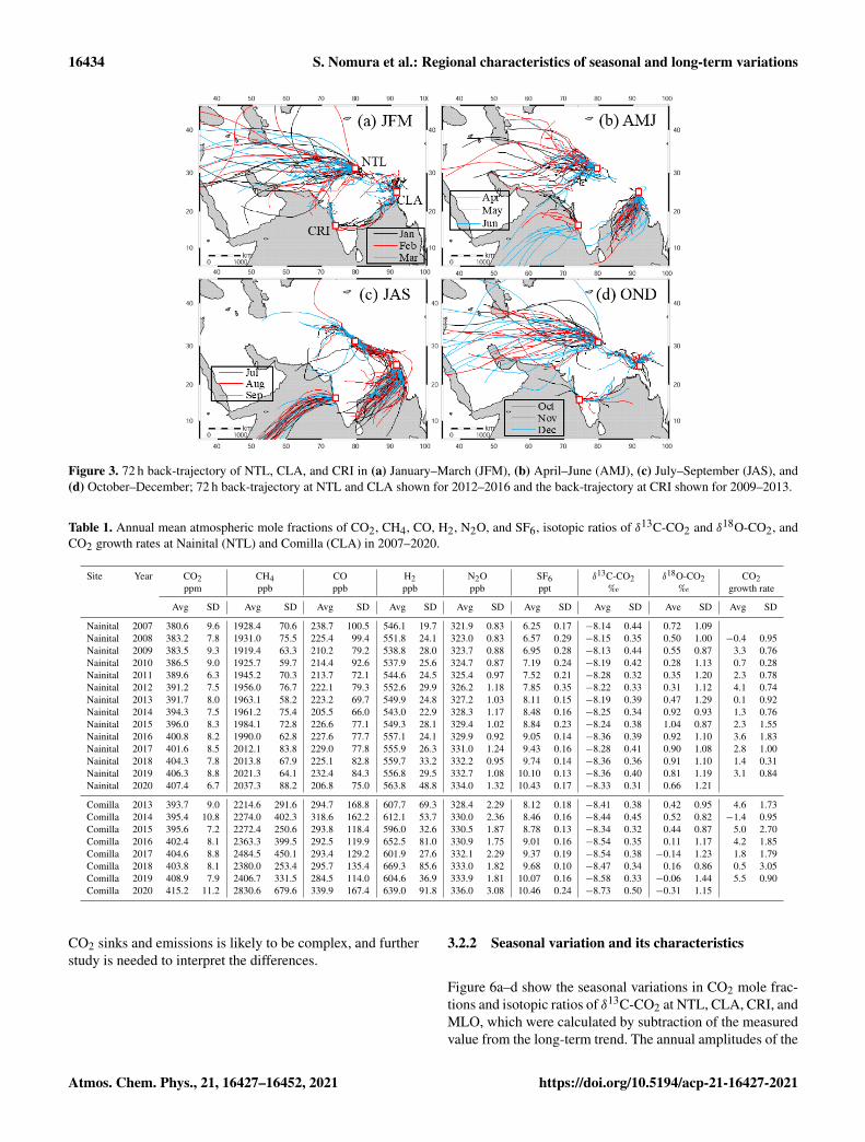
Basically, the air masses over the Indian subcontinent weretransported from the Indian Ocean region during summer(monsoon season) and from the inland during winter. Airmass trajectories are shown for our sampling sites and relatedsites in Fig. 3. In the case of anthropogenic GHGs, exceptCO2, their mole fractions at CLA generally showed relativelylow values when the air mass came from the ocean, while themole fractions were relatively high when the air mass camefrom inland. On the other hand, mole fractions of GHGs atNTL overall did not show relatively low values even if theair mass came from the Indian Ocean region (i.e., southeast-erly wind) because the air mass from the Indian Ocean was


http://hydro.imd.gov.in/hydrometweb/(S(fqu5hsvtq3sitn45rjia4qma))/landing.aspx

http://hydro.imd.gov.in/hydrometweb/(S(fqu5hsvtq3sitn45rjia4qma))/landing.aspx

http://www.data.jma.go.jp/gmd/cpd/monitor/climatview/frame.php?y=2019&m=7&d=30&e=0

http://www.data.jma.go.jp/gmd/cpd/monitor/climatview/frame.php?y=2019&m=7&d=30&e=0

http://db.cger.nies.go.jp/metex/index.html

http://db.cger.nies.go.jp/metex/index.html


strongly affected by local GHG emissions while passing overthe Indo-Gangetic Plain. However, the CO2 mole fractionchanged not only due to transport, but also due to the pho-tosynthetic sink strength of terrestrial ecosystems and culti-vated crops.

Annual mean GHG mole fractions at NTL and CLA aresummarized in Table 1. Annual CO2 mole fractions at bothsites were quite low compared to MLO and other Indian sitessuch as CRI. For example, in 2010, 386.5 ppm was reportedat NTL, 391.9 ppm at CRI (Bhattacharya et al., 2009), and391.3 ppm at PON (Lin et al., 2015). Note that there are nodata for CLA in 2010; however, the annual CO2 mole frac-tion at CLA is usually only 1–2 ppm higher than at NTL. Thisseemed to be due to the influence of photosynthesis at bothsites. Generally, the CO2 mole fractions at NTL and CLAdecreased strongly (typically twice a year) due to photosyn-thesis of local crops, making the annual CO2 mole fractionslower than at other sites despite the likelihood that anthro-pogenic emissions are high in this area.

On the other hand, the annual mean mole fractions of CH4,CO, H2, and N2O at NTL and CLA (Table 1) were almost atthe highest levels on the Indian subcontinent due to the in-fluence of strong emission sources. For example, the annualmole fractions of NTL and CLA were 50–470 ppb for CH4,30–200 ppb for CO, and 0–5 ppb for N2O higher compared toother Indian sites (e.g., CRI, Bhattacharya et al., 2009; HLE,PON, and PBL, Lin et al., 2015). In this region, high CH4and N2O emissions were possible from paddy fields and cul-tivated areas. Also, much CO is considered to be produced bybiomass burning in this region. As for H2, the mole fractionat CLA was higher than those at other Indian sites; however,it was relatively low at NTL compared to other sites suchas CRI (Bhattacharya et al., 2009), PON, and PBL (Lin etal., 2015) but similar to HLE, which is located on a highermountain. In the case of the SF6 mole fraction, it has smallerregional differences, suggesting there are no remarkable SF6sources near the measurement sites. Below we describe indetail the characteristics of sources and sinks of each com-ponent (CO2, δ13C-CO2, δ18O-CO2 CH4, CO, H2, N2O, andSF6) at NTL and CLA on the Indo-Gangetic Plain in termsof seasonal variations, amplitudes, and growth rates.

3.2 CO2 and δ13C-CO2

3.2.1 CO2 mole fraction and growth rate variations

Figure 4 shows the time series of the atmospheric CO2 molefraction and the isotopic ratio of δ13C-CO2 at our sam-pling sites (NTL and CLA) together with data from CRI onthe western coast of India and MLO in Hawaii. The CO2mole fractions at NTL and CLA in August–October werecharacteristically lower (approximately 10–20 ppm) than themole fractions observed at CRI and MLO. The CRI andMLO sites are representative of CO2 mole fractions in theSouthern Hemisphere and Northern Hemisphere, respec-

tively, for the period of the southwestern monsoon season(June–September). On the other hand, the δ13C-CO2 at NTLand CLA was inversely correlated with the CO2 mole frac-tions, and generally the values at both sites were higher thanat MLO and CRI.

Air masses at NTL and CLA in August–October passedover the Indo-Gangetic Plain and the southeastern area ofIndia, respectively, while the air masses of CRI were trans-ported from the Indian Ocean region (Fig. 3). Thus, it wassuggested that the air mass from the Indian Ocean in August–October prevailing over CRI was hardly influenced by an-thropogenic emission and photosynthesis over the Indiansubcontinent, whereas CO2 mole fractions over NTL andCLA seemed to be influenced during these seasons by thesources and sinks on the Indo-Gangetic Plain and the south-ern/eastern areas of the Indian subcontinent. Such transportcharacteristics must affect the annual average and growthrates in the CO2 molar ratio and δ13C-CO2 in addition totheir seasonal variations.

We show the CO2 growth rates observed at NTL, CLA,and MLO in Fig. 5a. Mean CO2 growth rates at NTL (ap-proximately 2.1 ppm yr−1 during 2007–2020) and CLA (ap-proximately 2.9 ppm yr−1 during 2013–2020) were similarto other sites (e.g., MLO). However, variations of the cal-culated growth rates were greater than those at MLO. Therange was 0–5 ppm yr−1 in the case of NTL, and CLA hadhigher variability than NTL because local sink and sourceinfluences affected the concentration more than remote sitessuch as MLO. In general, Pacific sites such as MLO andJapanese remote sites in the Northern Hemisphere showeda relationship between CO2 growth rates and the ENSO in-dex (e.g., Keeling, 1998). This relationship is often explainedfrom the viewpoint of a global temperature anomaly, whichhas a strong relationship with the ENSO index. On the otherhand, the variability at NTL has no associations with thevariability in the CO2 growth rate at MLO and the ENSOindex (Fig. 5b). Both growth rates seemed to be slightly in-versely correlated with each other from 2007 to 2015. How-ever, since then, similar relatively high growth rates havebeen observed for both sites around 2015–2016 and 2018–2019, indicating that, overall, the CO2 growth rate at NTLis less correlated with the CO2 growth rate at MLO and theENSO index.

It is well known that the Indian Ocean Dipole controls me-teorological conditions such as air mass transportation andprecipitation patterns on the Indian subcontinent (e.g., Sajiet al., 1999; Ashok et al., 2004; Hong et al., 2008). Suchchanges in regional climatic pattern could affect the CO2 up-take flux by plants in the surrounding area and the atmo-spheric movement, leading to a change in the CO2 growthrate. However, we did not find a simple relationship betweenDMI and CO2 growth rate at NTL (Fig. 5b). Here we haveshown that the pattern of CO2 growth rate in this region isdifferent from the global pattern seen in places like MLO, butthe relationship between local climatic factors and changes in



Figure 3. 72 h back-trajectory of NTL, CLA, and CRI in (a) January–March (JFM), (b) April–June (AMJ), (c) July–September (JAS), and(d) October–December; 72 h back-trajectory at NTL and CLA shown for 2012–2016 and the back-trajectory at CRI shown for 2009–2013.

Table 1. Annual mean atmospheric mole fractions of CO2, CH4, CO, H2, N2O, and SF6, isotopic ratios of δ13C-CO2 and δ18O-CO2, andCO2 growth rates at Nainital (NTL) and Comilla (CLA) in 2007–2020.

Site Year CO2 CH4 CO H2 N2O SF6 δ13C-CO2 δ18O-CO2 CO2ppm ppb ppb ppb ppb ppt ‰ ‰ growth rate

Avg SD Avg SD Avg SD Avg SD Avg SD Avg SD Avg SD Ave SD Avg SD

Nainital 2007 380.6 9.6 1928.4 70.6 238.7 100.5 546.1 19.7 321.9 0.83 6.25 0.17 −8.14 0.44 0.72 1.09Nainital 2008 383.2 7.8 1931.0 75.5 225.4 99.4 551.8 24.1 323.0 0.83 6.57 0.29 −8.15 0.35 0.50 1.00 −0.4 0.95Nainital 2009 383.5 9.3 1919.4 63.3 210.2 79.2 538.8 28.0 323.7 0.88 6.95 0.28 −8.13 0.44 0.55 0.87 3.3 0.76Nainital 2010 386.5 9.0 1925.7 59.7 214.4 92.6 537.9 25.6 324.7 0.87 7.19 0.24 −8.19 0.42 0.28 1.13 0.7 0.28Nainital 2011 389.6 6.3 1945.2 70.3 213.7 72.1 544.6 24.5 325.4 0.97 7.52 0.21 −8.28 0.32 0.35 1.20 2.3 0.78Nainital 2012 391.2 7.5 1956.0 76.7 222.1 79.3 552.6 29.9 326.2 1.18 7.85 0.35 −8.22 0.33 0.31 1.12 4.1 0.74Nainital 2013 391.7 8.0 1963.1 58.2 223.2 69.7 549.9 24.8 327.2 1.03 8.11 0.15 −8.19 0.39 0.47 1.29 0.1 0.92Nainital 2014 394.3 7.5 1961.2 75.4 205.5 66.0 543.0 22.9 328.3 1.17 8.48 0.16 −8.25 0.34 0.92 0.93 1.3 0.76Nainital 2015 396.0 8.3 1984.1 72.8 226.6 77.1 549.3 28.1 329.4 1.02 8.84 0.23 −8.24 0.38 1.04 0.87 2.3 1.55Nainital 2016 400.8 8.2 1990.0 62.8 227.6 77.7 557.1 24.1 329.9 0.92 9.05 0.14 −8.36 0.39 0.92 1.10 3.6 1.83Nainital 2017 401.6 8.5 2012.1 83.8 229.0 77.8 555.9 26.3 331.0 1.24 9.43 0.16 −8.28 0.41 0.90 1.08 2.8 1.00Nainital 2018 404.3 7.8 2013.8 67.9 225.1 82.8 559.7 33.2 332.2 0.95 9.74 0.14 −8.36 0.36 0.91 1.10 1.4 0.31Nainital 2019 406.3 8.8 2021.3 64.1 232.4 84.3 556.8 29.5 332.7 1.08 10.10 0.13 −8.36 0.40 0.81 1.19 3.1 0.84Nainital 2020 407.4 6.7 2037.3 88.2 206.8 75.0 563.8 48.8 334.0 1.32 10.43 0.17 −8.33 0.31 0.66 1.21

Comilla 2013 393.7 9.0 2214.6 291.6 294.7 168.8 607.7 69.3 328.4 2.29 8.12 0.18 −8.41 0.38 0.42 0.95 4.6 1.73Comilla 2014 395.4 10.8 2274.0 402.3 318.6 162.2 612.1 53.7 330.0 2.36 8.46 0.16 −8.44 0.45 0.52 0.82 −1.4 0.95Comilla 2015 395.6 7.2 2272.4 250.6 293.8 118.4 596.0 32.6 330.5 1.87 8.78 0.13 −8.34 0.32 0.44 0.87 5.0 2.70Comilla 2016 402.4 8.1 2363.3 399.5 292.5 119.9 652.5 81.0 330.9 1.75 9.01 0.16 −8.54 0.35 0.11 1.17 4.2 1.85Comilla 2017 404.6 8.8 2484.5 450.1 293.4 129.2 601.9 27.6 332.1 2.29 9.37 0.19 −8.54 0.38 −0.14 1.23 1.8 1.79Comilla 2018 403.8 8.1 2380.0 253.4 295.7 135.4 669.3 85.6 333.0 1.82 9.68 0.10 −8.47 0.34 0.16 0.86 0.5 3.05Comilla 2019 408.9 7.9 2406.7 331.5 284.5 114.0 604.6 36.9 333.9 1.81 10.07 0.16 −8.58 0.33 −0.06 1.44 5.5 0.90Comilla 2020 415.2 11.2 2830.6 679.6 339.9 167.4 639.0 91.8 336.0 3.08 10.46 0.24 −8.73 0.50 −0.31 1.15

CO2 sinks and emissions is likely to be complex, and furtherstudy is needed to interpret the differences.

3.2.2 Seasonal variation and its characteristics

Figure 6a–d show the seasonal variations in CO2 mole frac-tions and isotopic ratios of δ13C-CO2 at NTL, CLA, CRI, andMLO, which were calculated by subtraction of the measuredvalue from the long-term trend. The annual amplitudes of the



Figure 4. Time series of the (a) atmospheric CO2 mole fraction and the (b) isotope ratio of δ13C-CO2 at NTL, CLA, CRI, and MLO in2006–2020.

Figure 5. (a) Growth rates of the CO2 mole fraction at NTL, CLA, and MLO in 2006–2020 and (b) the El Niño–Southern Oscillation(ENSO) index in 2006–2020 and the Dipole Mode Index (DMI) in 2006–2020.

CO2 mole fraction (Table 2) at NTL (22.1± 3.9 ppm) andCLA (20.3± 5.7 ppm) were much larger than those at otherIndian sites (CRI, 15 ppm; HLE, 8.2 ppm; PON, 7.6 ppm;PBL, 11.1 ppm). Also, the annual amplitudes of δ13C-CO2at NTL (0.96 ‰± 0.16 ‰) and CLA (0.85 ‰± 0.19 ‰) werelarger than that at CRI (approximately 0.6 ‰). These resultssuggested that the atmospheric CO2 mole fractions of NTLand CLA were strongly influenced by photosynthesis of lo-

cal plants in summer and their respiration in winter and otheranthropogenic emissions which were moderated at the othersites by the influence of the oceanic air. Also, small episodicpeaks of the atmospheric CO2 mole fraction and isotopic ra-tio of δ13C-CO2 of CLA at the beginning of each year wereinfluenced by the biomass burning for heating in the close re-gion, which is considered to be the inland area from the siteaccording to the air trajectory analysis.



Table 2. Mean annual amplitudes of seasonal variation in atmospheric mole fractions of CO2, CH4, CO, H2, N2O, and SF6 and δ13C-CO2and δ18O-CO2 at NTL during 2007–2020 and at CLA during 2013–2020.

Site CO2 CH4 CO H2 N2O SF6 δ13C-CO2 δ18O-CO2ppm ppb ppb ppb ppb ppt ‰ ‰

Nainital 22.1± 3.9 114± 52 153± 44 50.3± 18.0 1.01± 0.74 0.18± 0.16 0.96± 0.16 2.71± 0.79Comilla 20.3± 5.7 486± 225 356± 90 70.4± 41.2 4.25± 1.45 0.23± 0.08 0.85± 0.19 2.33± 0.49

Figure 6. Seasonal variations in the CO2 mole fraction at (a) NTL and (b) CLA and the isotope ratio of δ13C-CO2 at (c) NTL and (d) CLA.Boxes with blue and red are for Nainital and Comilla, and the black and yellow lines are for MLO and CRI, respectively. Median values (theline in the box) and the inner 50th percentile of the value (box) and inner 90th percentile of the value are from the monthly averaged CO2mole fractions.

As shown in Figs. 4a and b and 6b and d, the seasonalvariation pattern at CLA has two lower seasons in CO2 andtwo higher seasons in δ13C-CO2 in February–April and July–October. Similarly, in the case of NTL, we sometimes ob-served relatively low mole fractions of CO2 in February–March and September and higher δ13C-CO2. In general,in many cases, including at MLO, only a summer mini-mum CO2 mole fraction is observed, while a minimum inFebruary–March is not usually observed.

Twice-yearly decreases in the CO2 mole fraction havealso been observed at several Indian sites such as Dehradun(northern Indian site; Sharma et al., 2013), Sinhagad (west-ern Ghats site; Tiwari et al., 2014), Ahmedabad (western In-dian site; Chandra et al., 2016), Shadnagar (central Indiansite; Sreenivas et al., 2016), and PON (southeastern coastalIndian site; Lin et al., 2015); however, these studies did notclearly mention such variations. Umezawa et al. (2016) re-ported that the decrease in the CO2 mole fraction near theground in February–March was caused by photosynthesis oflocal crops, which was detected by the vertical CO2 profilesover New Delhi Airport. Those sites are located on the Indo-Gangetic Plain or received air masses passing over the Indo-

Gangetic Plain or Indian subcontinent. On the other hand,the decrease in the CO2 mole fraction in February–Marchwas not detected at CRI (western coastal Indian site; Bhat-tacharya et al., 2009), HLE (northwestern Himalayan site),or PBL (Andaman Islands site) (Lin et al., 2015). These sitesare not located on the Indo-Gangetic Plain. Thus, air massesat these sites must be mainly transported from the ocean orfrom areas other than the Indian subcontinent during theseperiods.

The characteristic CO2 seasonal variation on the Indo-Gangetic Plain (including NTL and CLA) is very likely tobe related to CO2 uptake by regional vegetation. Generally,in the case of the state of Uttar Pradesh located in the cen-ter of the Indo-Gangetic Plain, rice and other summer plants(maize, millets, etc.) are planted mainly in June–July and har-vested in October–November, while large areas of wheat aresown in October–December and harvested in March–April.Therefore, relatively low CO2 mole fractions observed inthose periods are considered to be due to CO2 uptake byplants cultivated in each season near NTL.

In Bangladesh, rice, being the staple food, is cultivatedthree times a year in some regions. Usually rice is grown



twice (aus and amon rice) from April to October (includ-ing the monsoon season); however, rice is also often cul-tivated (boro rice) in the winter season from November toApril (SID/MP, 2018). Other agricultural products includemaize, jute, and vegetables in the summer season and a smallamount of wheat in the winter season. Therefore, we con-cluded that the observed lower CO2 mole fractions in July–October and February–March were influenced by CO2 up-take by local plants (mainly rice). Especially at CLA, thelower mole fraction in February–March was clear, and astrong contribution from CO2 uptake from boro rice was es-timated. As another viewpoint on CO2 seasonal variation,we observed that the CO2 maximum in May was not sohigh, while the CO2 mole fraction in December was higher.Because precipitation in Bangladesh is stronger than in thenorthern Indian region, the duration of rice cultivation oversummertime is also longer than in northern India. Therefore,the contribution of plant uptake to the CO2 mole fraction inthe atmosphere at CLA over the summer season is likely tobe relatively large compared to that at NTL.

Thus, the decreases in the CO2 mole fractions inFebruary–March and September in NTL and CLA were es-timated to be caused by photosynthesis of plants cultivatedin each season over the Indo-Gangetic Plain. NTL and CLAindicated this more clearly compared with other Indian sitesdue to the proximity to the source region. Figure 7a showsthe relationships between the annual mean CO2 mole frac-tion and δ13C-CO2 in 2010 and 2012. The slope betweenthe CO2 mole fraction and δ13C-CO2 showed −0.050 and−0.054 ‰ ppm−1, which indicated that the spatial variabil-ity of the atmospheric CO2 mole fraction (e.g., a lower molefraction at NTL than at MLO and CRI) basically occurreddue to CO2 exchange between the atmosphere and terrestrialbiosphere.

Furthermore, we examined the relationship of the CO2mole fraction and carbon isotope ratio, because there aresome seasonal differences in the species cultivation. Onthe Indo-Gangetic Plain, rice (especially in Bangladesh)and wheat (especially in northern India), as C3 plants, arecultivated in January–March, while C4 plants, e.g., maize,sugarcane, sorghum, and bajra (pearl millet), in additionto rice are cultivated on the Indo-Gangetic Plain and inBangladesh in June–September (DAC/MA, 2015; SID/MP,2018; DES/MAFW, 2019). We calculated the end-memberof the isotope value for absorbed CO2 by using intercept val-ues of the Keeling plot between the reciprocal of the CO2mole fraction and the ratio of δ13C-CO2 obtained from twocontinuous datasets of air samples, which has> 1 ppm differ-ence in CO2 mole fraction and> 0.05 ‰ in δ13C-CO2. Sincein this study two datasets had 1-week intervals, we assumedthat the difference in CO2 and δ13C between two datasetswould include broader influences of photosynthetic activitiesfrom relatively large areas on the Indo-Gangetic Plain.

We found that the intercept values of NTL and CLAshowed differences in January–March and June–September

(Fig. 7b), which appeared to reflect the differences in thecontributions of C3 and C4 plants in this region. In June–September, we found relatively heavier intercept values atboth NTL (−25.0 ‰± 2.4 ‰) and CLA (−23.5 ‰± 4.1 ‰),suggesting that C4 plants partly contributed to the CO2 ab-sorption (or emission) in this season, while in January–March, the end-member showed −29.0 ‰± 4.3 ‰ (NTL)and−28.3 ‰± 4.0 ‰ (CLA), which were similar to the gen-eral C3 plant (rice or wheat). If we assume the value for theC4 plant to be −12 ‰ to −14 ‰, the contributions of theC4 plant in NTL and CLA were approximately 25 %± 5 %and 31 %± 9 %, respectively. According to the database(DAC/MA, 2015; SID/MP, 2018; DES/MAFW, 2019) forcrop area in Uttar Pradesh, the area’s ratio of C4 plants (e.g.,maize and sugarcane) to C3 plants in the summer seasonwas approximately 26 % in 2012, which was a similar pro-portion to that estimated by the C isotope ratio. In the caseof Bangladesh, despite there being no recent data reported,according to data in 2008, the area for maize was approxi-mately< 10 % compared to the rice area. However, based onthe recent C isotope ratio, it appears likely that more maizehas been cultivated.

3.3 δ18O-CO2

In general, δ18O-CO2 is related to that value of water inplants and soil, because oxygen atoms of CO2 can be ex-changed with oxygen atoms of H2O in plant and bacteriacells during photosynthesis and soil respiration. Plants andsoil water mainly originate from rainwater in the study re-gion; however, in the case of the agricultural area, water isoften introduced by irrigation systems using river water andgroundwater. In many cases, photosynthesis produced rela-tively heavier δ18O-CO2 than soil respiration because δ18O-H2O in plants becomes heavier than soil water due to planttranspiration.

Larger amplitudes (approximately 3 ‰) in the seasonalvariation of δ18O-CO2 at both NTL and CLA were observedcompared to that of MLO (approximately 0.4 ‰) (Fig. 8a).The isotopic ratio of δ18O-CO2 at CRI (Bhattacharya et al.,2009) was reported to have similar seasonal variation (i.e.,high in winter (November–February) and low in September)to our sites. In the Pacific sites like MLO, δ18O-CO2 has amaximum peak from spring to summer, when photosynthesisactivity becomes dominant, while a minimum is seen aroundfall, when the contribution of soil respiration exceeds that ofphotosynthesis. On the other hand, Indian subcontinent sitesseemed to have fairly different seasonal variation patterns,with a maximum in January–February, gradually decreasingfrom March to September/October and subsequently rapidlyincreasing (Fig. 8c and d). Such seasonal variation may beinfluenced by photosynthesis and soil respiration in these re-gions. However, because many crops are cultivated throughthe year in these areas (as mentioned in Sect. 3.2), the con-tribution of photosynthesis to the seasonal variation may be



Figure 7. (a) Relationship between the annual values of the CO2 mole fraction and isotopic ratio of δ13C-CO2 at NTL, CRI, and MLO in2010 and 2012 and (b) the intercept values of the Keeling plot of NTL and CLA in January–March and June–September.

relatively small. High soil respiration activity in the wet sea-son can contribute a little more than during the dry season.

On the other hand, seasonal variations in δ18O of rain-water itself seemed to affect δ18O-CO2 through photosyn-thesis and respiration processes. For example, Sengupta andSarkar (2006) showed that the δ18O-H2O in rain at NewDelhi (western Indo-Gangetic Plain) had a higher value inMarch–May and a minimum value in September. Such vari-ation was fairly consistent with the seasonal variation inδ18O of CO2 at NTL. Similarly, CLA has a minimum δ18O-CO2 in the atmosphere in October, which was the samemonth in which the minimum δ18O-H2O was observed inrain in eastern Indo-Gangetic Plain areas (e.g., Kolkata nearBangladesh, Sengupta and Sarkar, 2006; Cherrapunij, east-ern Indo-Gangetic Plain; Breitenbach et al., 2010). Duringthe rainy season, due to the so-called “amount effect”, δ18O-H2O in rain will decrease with an increase in the amount ofprecipitation (e.g., Rozanski et al., 1993). However, in theIndian region it has been reported that seasonal changes inthe origin of moisture strongly affected the δ18O-H2O (Sen-gupta and Sarkar, 2006; Tanoue et al., 2018). In winter (i.e.,when there is less rain), moisture comes from the west ornorth. Therefore, the northern area of the Arabian Sea and thewestern land area supply moisture, which has a higher δ18O-H2O. However, the air mass in the summer monsoon season(mainly June–September) comes from the southern part ofthe Arabian Sea and sometimes passes over the Bay of Ben-gal, carrying much moisture. The value of δ18O-H2O in themoisture in the air mass decreases with the process of rainingalong the air trajectory. In the post-monsoon season (mainlyOctober–December), some portion of moisture comes from

the Pacific, Bay of Bengal, and inland area (Tanoue et al.,2018).

In the winter monsoon season (mainly February–May),δ18O-H2O in rain was reported to be approximately 0 ‰–1 ‰ (vs. VSMOW). During the winter monsoon season,there is little precipitation, so plant cultivation utilizes irriga-tion systems using river water and groundwater. River waterand groundwater usually show not so large seasonal varia-tion in δ18O and have a value close to the annual mean ofδ18O-H2O in rain, such as −6 ‰ to −8 ‰ (Kumar et al.,2019). According to the variation of δ18O-CO2, in winter itsvalue was approximately 2 ‰ (vs. VPDB-CO2; the VPDB-CO2 scale is fairly close to the scale of CO2 equilibrated withVSMOW, as mentioned in Sect. 2.3), which was higher thanthat of rain and other water reservoirs, suggesting that δ18O-H2O in plants and soil must become higher due to transpira-tion during dry and relatively warm conditions in winter.

Based on the fact that, during the summer monsoon sea-son, δ18O-CO2 decreased from 1 ‰ to−2 ‰ with a decreasein δ18O-H2O from 0 ‰ to −10 ‰ or −15 ‰ in the rain, therange of variation in δ18O-CO2 was approximately one-thirdor one-fifth that of rain. Because land water may come fromboth rain and irrigation systems, the real ranges of δ18O insoil water and plant water are likely to be smaller than inthe case of rain only. Furthermore, because CO2 from soilrespiration contributes more in the rainy season, a balancebetween photosynthesis and respiration CO2 will, in general,have a small effect on the seasonal variation.

As for the annual trend of δ18O-CO2 shown in Fig. 8b,NTL showed a similar pattern to that of MLO, whereas CLAshowed a different trend. The δ18O-CO2 at NTL began at0.8 ‰ in 2007, decreased to 0.2 ‰ in 2011, and then again



Figure 8. Time series of (a) measured values and (b) the long-term trend for the isotopic ratio of δ18O-CO2 at NTL, CLA, and MLO in2006–2020, the seasonal variation of δ18O-CO2 at (c) NTL and (d) CLA, and the relationship between monthly precipitation of the state ofUttarakhand and Bangladesh and the monthly mean of δ18O-CO2 at (e) NTL and (f) CLA.



became heavier (toward 1.0 ‰) during 2014–2016 (Fig. 8b).In northern India, relatively high precipitation was reportedduring 2011–2013. The tendency of lower δ18O-CO2 mayhave some relationship with the amount of precipitation. In2008 and 2016 considerable amounts of precipitation fellnear NTL. The δ18O-CO2 level also seemed to become rela-tively low. A La Niña event occurred from late 2010 to 2012,and the amount of precipitation increased worldwide from2010 to 2013. Such large-scale climatic effects are very likelyto affect the δ18O-CO2 level observed at MLO. In the case ofCLA, precipitation increased in 2015–2017 and 2019–2020(rather than in 2011–2013), and the δ18O-CO2 level at CLAseemed to become lower at that time with the increase in pre-cipitation. Analyzing the relationship between the monthlyamount of precipitation and δ18O-CO2 in Fig. 8e and f, aweak negative correlation can be seen (if the monthly meanδ18O-CO2 at CLA adds 1 or 2 months of time lag to themonthly mean of the precipitation, the correlation coefficient(R2) between the monthly mean δ18O-CO2 at CLA and themonthly mean of precipitation increases to be 0.4 or 0.5).Therefore, the amount of precipitation partly contributes tothe regional level of δ18O-CO2. However, it must be influ-enced not only by precipitation, but also by seasonal changesin air flow patterns and rain systems, as explained above, aswell as by the water reservoir situation, soil water content atthat time, and photosynthesis in the region.

If the groundwater storage decreases due to wider usage ofirrigation and/or less precipitation in recent times, it causes astronger transpiration effect in the soil environment, makingthe δ18O of soil water heavier than usual. Roxy et al. (2015)and Asoka et al. (2017) reported that precipitation over theIndian subcontinent and groundwater storage in northern In-dia have had a decreasing trend due to Indian Ocean warm-ing, which is estimated to have occurred due to the weak-ening trend of the summer monsoon cross-equatorial flow(Swapna et al., 2014). However, much longer records of CO2isotopic ratios are needed to clarify the increasing trend inδ18O-CO2 and the relationship with climatic changes in thisregion.

3.4 CH4

The CH4 mole fractions at NTL and CLA are illustrated inFig. 9a. We detected high CH4 mole fractions at NTL andCLA, where they sometimes exceeded 2100 and 4000 ppb,respectively, showing that the Indo-Gangetic Plain regionhad relatively strong CH4 emissions. The seasonal amplitudeof the CH4 mole fraction, especially at CLA (486± 225 ppb;Table 2), was much larger than those of other Indian sitessuch as NTL (114 ppb), CRI (200 ppb) (Bhattacharya et al.,2009), Darjeeling (400 ppb) (Ganesan et al., 2013), HLE(29 ppb), PON (124 ppb), and PBL (144 ppb) (Lin et al.,2015), which indicated that the contribution of the CH4source (e.g., rice cultivation) around CLA was relativelystrong. Mean seasonal variations in the CH4 mole fraction

for both sites were calculated and are shown in Fig. 9c andd. The mole fractions at both NTL and CLA had the highestpeak in August–October and a small peak in March. In gen-eral, the CH4 mole fraction in the Northern Hemisphere de-creased in July–September (summer season) through the de-composition process by reaction with OH radicals during thisperiod. A higher CH4 mole fraction in this period stronglysuggests that there are some sources of CH4. Observationresults at Darjeeling (northeastern Indian site; Ganesan etal., 2013), HLE (Lin et al., 2015), and Shadnagar (Sreenivaset al., 2016) also indicated high CH4 mole fractions duringAugust–October. Ganesan et al. (2013) reported that the CH4mole fraction at Darjeeling was enhanced by transported airmasses from the Indo-Gangetic Plain. Lin et al. (2015) andSreenivas et al. (2016) showed that the high CH4 mole frac-tions at HLE and Shadnagar were influenced by emissionsfrom paddy fields and wetlands. Garg et al. (2011) showedthat CH4 emission from rice fields was estimated to be ap-proximately 17 % of the total CH4 emissions in India. Ac-cording to the emission database of EDGAR v4.3.2 (EC-JRC/PBL, 2016), rice cultivation was the largest source ofCH4 (approximately 50 %) in Bangladesh.

Bhatia et al. (2011) measured the CH4 flux from paddyfields at New Delhi and showed that it was the highest inAugust–September due to the increase in the activity of riceroots and bacteria in the paddy field soils. Ali et al. (2012)also measured the CH4 flux from paddy fields at Bangladeshand reported that the CH4 flux was maximized within 77–98 d after the planting of rice due to the increase in rootrespiration and carbon in soil. It was considered that bothMarch and September–October were consistent with the tim-ing of increasing CH4 production at rice fields according tothe customary cultivation schedule of rice in this region. InBangladesh and the eastern Indian district, rice is cultivatedfrom November to September, as mentioned above in theCO2 section, and CH4 emissions are considered to continueduring winter, supporting higher CH4 mole fractions fromAugust to March, especially at CLA.

On the other hand, CRI (Bhattacharya et al., 2009), PON,and PBL (Lin et al., 2015) did not show higher CH4 molefractions in August–October, as shown in Fig. 9c and d. Theair masses at those sites in August–October were transportedfrom the Indian Ocean, which may have only a minimal in-fluence from agricultural emission.

CH4 mole fractions at NTL and CLA were higher than thatat MLO, even at the time of year when rice is not cultivated.CH4 emissions from the enteric fermentation and wastewaterhandling were reported to be large sources according to theemission database in EDGAR v4.3.2 (EC-JRC/PBL, 2016).Garg et al. (2011) reported that enteric fermentation by cat-tle and buffalo contributes approximately 40 % of emissionsin India. Such CH4 emissions must always elevate the CH4mole fraction in the air mass in these sites regardless of theseason.



Figure 9. Time series of (a) measured values and (b) growth rates of the CH4 mole fraction at NTL, CLA, CRI, and MLO in 2006–2020, theseasonal variation in the CH4 mole fraction at (c) NTL and (d) CLA, and the relationship between the short-term components of dCO anddCH4 at (e) NTL and (f) CLA during January–March (JFM), April–June (AMJ), July–September (JAS), and October–December (OND).



In addition, biomass burning (including residential cook-ing and agricultural residue burning) is very likely to havea contribution to the CH4 mole fraction according to the in-ventory evaluation (i.e., 21 % contribution; Garg et al., 2011).Reasonably good correlations were seen between short-termcomponents in variations of CH4 and CO in January–March,April–June, and October–December. Ratios of dCH4 to dCOshowed ranges such as 0.64–0.80 ppb ppb−1 in NTL and1.85–1.98 ppb ppb−1 in CLA, as shown in Fig. 9e and f.One of the major CO sources in India was considered to bebiomass burning (Dickerson et al., 2002). Akagi et al. (2011),EC-JRC/PBL (2016), and Sfez et al. (2017) reported that theemission ratios of CH4 to CO in biomass burning such ascrop residue burning, firewood burning, and biogas burningwere 0.04–0.90 ppb ppb−1. Therefore, the ratios observed inthese seasons could suggest a strong influence on CH4 andCO emissions from biomass burning (such as crop residueburning), despite the other large CH4 emissions such aspaddy fields and waste treatment, which will increase the ra-tio, especially at CLA in July–September.

As a result, it is evident that annual CH4 mole fractionsat the sites used in this study on the Indo-Gangetic Plain areenriched by various CH4 sources, depending on the season.Generally speaking, because April–June is a dry and hot sea-son, CH4 decomposition processes will proceed, decreasingits mole fraction at both sites.

The variability in the CH4 growth rate in the trend line atNTL was different to the variability at MLO (Fig. 9b), whichmay be influenced by regional climatic condition, includingthe Indian Ocean Dipole. Because the frequency of air masstransportation from the south increased if the Indian OceanDipole was often activated, the air mass passed over the Indo-Gangetic Plain (which has strong CH4 emissions), reachingNTL with a high CH4 mole fraction. The difference betweenthe variability in the CH4 growth rate between NTL and CLAmay also be explained by the above hypothesis. If the fre-quency of air mass transportation from the south increasedby the activation of the Indian Ocean Dipole (e.g., in 2015)because the air mass was directly transported from the IndianOcean with a relatively low CH4 mole fraction, the CH4 molefraction at CLA would become relatively low compared to ausual year (Fig. 9b). On the other hand, as mentioned previ-ously, in 2015–2017, even in the high Indian Ocean DipoleMode, Bangladesh had relatively high precipitation, whichcould strengthen CH4 production from rice paddy fields andother aquatic environments. This potential situation matchedthe high CH4 mole fraction well in summer and the highgrowth rate at CLA during 2016–2017.

3.5 CO

High annual CO mole fractions at both NTL and CLA (Ta-ble 1) indicated that the atmosphere over the Indo-GangeticPlain was influenced by strong CO emission sources suchas burning of harvest residues and residential burning using

solid biofuel, which are considered to be the main CO emis-sion sources in the region (EC-JRC/PBL, 2016). However, ofcourse, CO originating from car exhaust and industrial activ-ities remains very likely to have made some contributions tothe CO mole fraction (EC-JRC/PBL, 2016).

The main crops around NTL are rice and wheat, andthe harvesting periods are September–November and April–May, respectively (DAC/MA, 2015). Farmers in this areagenerally burn harvest residues at their farmland after harvest(Lohan et al., 2018). Venkataraman et al. (2006) reported thatthe amount of burning on the western Indo-Gangetic Plainhas two peaks annually, i.e., in May and November. We couldobserve the same seasonal variation in the CO mole fractionin the atmosphere at NTL (Fig. 10c). Kumar et al. (2011)also reported that the highest densities in fire spots were seenin spring and autumn on the western Indo-Gangetic Plain.These suggested that CO emissions from the burning of har-vest residues was one of the most important sources on thewestern Indo-Gangetic Plain in these seasons.

On the other hand, the seasonal variation in CO molefraction at CLA exhibited only one peak in October–March(Fig. 10d). Such seasonal variation was also detected at CRI(Bhattacharya et al., 2009), PON, PBL (Lin et al., 2015),and Ahmedabad (Chandra et al., 2016). In Bangladesh, afterthe end of the monsoon (October–March), harvest residuesare burnt and used to make bricks using some kinds of bio-fuel as a heat source (Guttikunda et al., 2013). Also, dungis burnt for the stove (Venkataraman et al., 2010) duringthe winter season. In addition, biofuel is used for cooking(Lawrence and Lelieveld, 2010) throughout the year. Thoseactivities could emit large amounts of CO (Streets et al.,2003; Venkataraman et al., 2010; Maithel et al., 2012).

In addition, the seasonal amplitude of the CO mole frac-tion (Table 2) at CLA (356± 90 ppb) at the eastern Indo-Gangetic Plain site was much larger than that observed atother Indian sites (e.g., CRI – 200 ppb, PON – 78 ppb, PBL –144 ppb, and Ahmedabad – 270 ppb). The highest CO ampli-tude observed at CLA was consistent with the model estima-tion of CO emissions, which showed that the eastern Indo-Gangetic Plain included areas with the highest CO emissions(Kumar et al., 2013).

On the other hand, the annual mean CO mole fractionat NTL gradually decreased approximately by 50 ppb for10 years (2006–2015; Fig. 10a). Especially the monthlymean CO mole fraction in November of each year (i.e., thehighest level in the year) at NTL decreased by 120 ppb duringthat period. This suggests that the amount of harvest residuesburnt decreased, the ratio of incomplete combustion in carengines was improved, or the type of fossil fuel for cookingchanged from biofuel to natural gas. Such decreasing trendsin the CO mole fraction level were also detected by Pandeyet al. (2017), who reported total-column CO levels during2003–2014 over the Indo-Gangetic Plain. However, the COmole fraction level at NTL appeared to increase slightly from2015. Although the reason for the increase is unclear from



Figure 10. Time series of (a) measured values and (b) growth rates of CO mole fractions at NTL, CLA, CRI, and MLO in 2006–2020 andthe seasonal variation of CO mole fractions at (c) NTL and (d) CLA.

this study only, CO emissions from car exhaust were recentlyestimated to have increased (EC-JRC/PBL, 2016). Therefore,further monitoring is important.

The trend in the CO mole fraction and its interannual vari-ability at NTL was similar to those in CH4 at NTL (Figs. 9band 10b). The mole fractions of CO and CH4 at NTL tendedto be slightly higher when the air mass passed over the Indo-Gangetic Plain, where there are strong sources of both COand CH4. In 2015 and 2017, a large positive Indian DipoleMode occurred in addition to El Niño in 2015. Therefore, weobserved more frequent southern winds, causing higher CH4

and CO mole fractions at NTL. However, at CLA, southernwind will decrease the mole fraction of CO. Thus, temporalvariations of both CO and CH4 mole fractions in both sitesmust be strongly controlled by meteorological conditions aswell as source strength.

3.6 H2

Mole fractions, growth rates, and seasonal variations of H2 atboth sites are shown in Fig. 11a–d. It was found that CLA, es-pecially, showed a higher mole fraction than the other sites.



Novelli et al. (1999) reported that the main sources of H2were combustion (fossil fuel combustion and biomass burn-ing) and photochemical sources such as the oxidation ofCH4 and non-CH4 hydrocarbons (NMHCs), which accountfor 90 % of the total source. The other 10 % is attributed toemissions from volcanoes, oceans, and nitrogen fixation bylegumes. Therefore, we have to assume that there are someemission sources at CLA.

On the other hand, H2 is removed from the troposphereby reacting with OH and by deposition and oxidation at sur-face soil. The amounts of sources and sinks for H2 in theglobal budget were estimated to be equal, resulting in a near-equilibrium state (Novelli et al., 1999). The strengths of H2removal in the atmosphere over the Indian subcontinent donot differ greatly by region according to Yashiro et al. (2011),whereas the strengths of H2 sources may differ by region(Price et al., 2007). Lin et al. (2015) reported that H2 molefractions at Indian sites were influenced by biomass burn-ing and were 0–40 ppb higher than those at regional back-ground sites (e.g., eastern Kazakhstan and central China).Figure 11c and d show the seasonal variations of the H2mole fraction at NTL and CLA, which illustrate the maxi-mum in May and the minimum in December at NTL and themaximum in November–January and the minimum in June–August at CLA, which were different from the averaged sea-sonal variation in the Northern Hemisphere, which showedthe maximum in March–April and the minimum in August–September (Novelli et al., 1999).

Because the burning of biomass (such as harvest residualsand dung) appeared to be actively carried out on the Indo-Gangetic Plain (including at NTL) during April–May andat CLA during November–February, H2 production must,therefore, increase during these seasons. Furthermore, sincehigher CH4 mole fractions at NTL and CLA were observedduring August–September and September–October due tostrong paddy field emissions at those times, H2 productionfrom CH4 degradation can also increase. Figure 11e and fshow short-term variable components (such as dCO and dH2,dCH4, and dH2) at both NTL and CLA during those pe-riods and that they had positive correlations. These figuresmay suggest some relationship between H2 emission withbiomass burning and between photochemical reactions be-tween OH and CH4, respectively. Furthermore, the minimumH2 in June–August was influenced by a fresh air mass fromthe Indian Ocean which is only minimally affected by an-thropogenic emission.

As mentioned above, the H2 mole fraction level at CLAwas higher than that at NTL. The amplitude of the seasonalvariation of the H2 mole fraction (Table 2) at CLA showed70.4± 42.2 ppb, which was also larger than the amplitudesat other Indian sites such as Nainital (50 ppb), CRI (50 ppb)(Bhattacharya et al., 2009), HLE (22 ppb), PON (16 ppb),and PBL (22 ppb) (Lin et al., 2015). These tendencies wereconsistent with the results of Price et al. (2007), which in-dicated a larger H2 emission area around the eastern Indo-

Gangetic Plain, such as at CLA, than in the western In-dian subcontinent. Thus, our observation and previous stud-ies both indicated that the Indian subcontinent had relativelystrong H2 sources.

3.7 N2O

Garg et al. (2012) reported that the agricultural sector ac-counted for approximately 75 % of the total N2O emissionin India in 2005, including around 49 % from nitrogen fertil-izer use. In particular, they reported that northern India (theIndo-Gangetic Plain) has the highest N2O emission in Indiabecause nitrogen fertilizer was applied to extensive paddyfields and was denitrified and that N2O was produced andemitted into the atmosphere. Ganesan et al. (2013) reportedthat the N2O mole fraction at Darjeeling (northeastern In-dian site) was enhanced due to air mass transportation fromthe Indo-Gangetic Plain. The annual mean N2O mole frac-tion at NTL (Table 1) appeared to be almost the same as atthe Darjeeling sites in northern India and was higher than atanother two Indian sites (CRI; Bhattacharya et al., 2009; andHLE; Lin et al., 2015) and at MLO (Fig. 12a).

Thompson et al. (2014) estimated that the N2O emissionsof the eastern Indo-Gangetic Plain, including CLA, werehigher than those of the western Indo-Gangetic Plain. This issupported by our observation results that show that the N2Oannual mean mole fraction during 2013–2019 at CLA on theeastern Indo-Gangetic Plain was 1–2 ppb higher than at NTLon the western Indo-Gangetic Plain (Table 1), and the sea-sonal amplitude of the N2O mole fraction (Table 2) at CLA(4.25± 1.45 ppb) was higher than the amplitudes at other In-dian sites (NTL; CRI, Bhattacharya et al., 2009; HLE; PON;and PBL, Lin et al., 2015). Raut et al. (2011) reported thehighest N2O emission rates in the regions of Bangladesh andSri Lanka due to their high usage of urea as a fertilizer.

However, interestingly, PON and PBL, where oceanic airfrom the Bay of Bengal affected the sites (Lin et al., 2015),seemed to have relatively higher mole fractions than the sitesin this study. As for the seasonal variation in the N2O molefraction at NTL, a higher mole fraction was seen in May–September (Fig. 12c). Generally, nitrogen fertilizer was fre-quently applied to paddy fields in May–September in north-ern India. Gupta et al. (2016) measured the N2O flux in paddyfields at New Delhi and reported that the flux increased im-mediately after the application of nitrogen fertilizer to thefields. Therefore, high N2O levels and increases in the N2Omole fraction at NTL in May–September were influenced bythe enhancement of the N2O flux due to the denitrification ofnitrogen fertilizer in paddy fields.

The N2O mole fraction at CLA increased in November–February (Fig. 12d), and such seasonal variation wasalmost identical to the seasonal variation in CO atCLA. The seasonal component in the N2O mole frac-tion (1N2O= deviation of the N2O mole fraction fromthe long-term trend) at CLA showed positive corre-



Figure 11. Time series of (a) measured values and (b) growth rate of the atmospheric H2 mole fraction at NTL, CLA, and CRI in 2006–2020and seasonal variation in the H2 mole fraction at (c) NTL and (d) CLA and scatter plots for the relationship of (e) 1H2 and 1CO at NTLduring April–May and at CLA during November–February when biomass burning occurred frequently, and (f) 1H2 and 1CH4 at NTLduring August–September and at CLA during September–October when the maximum CH4 mole fraction was measured.



Figure 12. Time series of (a) measured values and (b) growth rates of the N2O mole fraction at NTL, CLA, and MLO in 2006–2020, seasonalvariations in the N2O mole fraction at (c) NTL and (d) CLA, and (e) the relationship between the 1N2O and 1CO at CLA in 2013–2019.

lations (R2= 0.81− 0.88) with that of the CO mole

fraction (1CO) each year (Fig. 11e). Also, their ratio(1N2O /1CO) showed 0.013–0.015 ppb ppb−1, which wasthe same (0.015 ppb ppb−1) as the ratio of total N2O and to-tal CO emissions in Bangladesh from the EDGAR v4.3.2database (EC-JRC/PBL, 2016). Although such seasonal vari-

ation is likely to be partly related to the lower mixing heightin the winter season, variations in N2O emission flux mustaffect the seasonal variations in the mole fraction. In gen-eral, the CO mole fraction was influenced by biomass burn-ing in this season. Because many inventory data showedthat biomass burning produced both N2O and CO, N2O



may be affected partly by emission from biomass burn-ing. However, the emission ratios of N2O to CO are fairlyvariable, with an approximate range of 0.0004–0.017 (An-dreae and Merlet, 2001; Sahai et al., 2007, 2011; EDGARv4.3.2, EC-JRC/PBL, 2016). It seemed that this ratio changeswith the types of plants that are burnt. According to Sa-hai et al. (2011), because the ratio was approximately 0.004in the case of rice straw, some portion (e.g., 0.004/0.015,i.e., approximately 27 % at the most) of N2O in the atmo-sphere may originate from biomass burning. In addition,since Venkataraman et al. (2010) reported that dung burningis one of major N2O sources among many kinds of biomassburning in India, its contribution was also possible.

On the other hand, nitrification and denitrification pro-cesses of nitrogen fertilizer in rice paddy soil are consideredto be major causes of N2O emissions in this region (EDGARv4.3.2); however, the emission rate appeared to have seasonalvariation. Related to the irrigation system, the N2O flux wasthought to be larger in alternating wet and dry conditions thanunder continuously flooded conditions (Akiyama et al., 2005;Gaihre et al., 2018; Begum et al., 2019). In the summer mon-soon season, many rice paddy fields in Bangladesh must haveenough water level because of the ample amount of precipi-tation. After the summer monsoon (from October), the waterlevel in the paddy field intermittently changed with the situa-tion. Therefore, relatively, a higher N2O emission rate likelyoccurred during the winter season, when rice (boro rice) wasstill grown, enhancing the N2O mole fraction in the winterseason. Further observations of high-frequency variations ofboth N2O and CO mole fractions will contribute towards pre-cisely evaluating the N2O emission sources at this site.

The N2O growth rates at NTL and CLA were similar tothat of MLO (Fig. 12b); however, the variations in the N2Ogrowth rate at both NTL and CLA were larger than that ofMLO during 2016–2020. The variation in the N2O growthrate showed a similar pattern to the growth rates of CO andH2 (Figs. 9b and 10b), indicating that the sources of thesegases had basically common characteristics.

3.8 SF6

SF6 is mainly emitted artificially from factories and urbanareas (Olivier et al., 2005). Ganesan et al. (2013) reportedthat the SF6 emission at Darjeeling (northeastern Indian site)was considerably weak. Our results also showed that SF6mole fractions at NTL and CLA were almost the same as thebackground SF6 mole fraction (e.g., MLO in Fig. 13a andother sites such as HLE, PON, and PBL, Lin et al., 2015).In addition, the annual amplitudes of the SF6 mole fractionat Indian sites (HLE, PON, and PBL) were 0.15, 0.24, and0.48 ppt, respectively, which were almost within the samerange (0.15–0.23 ppt) as at NTL and CLA (Table 2). Theseresults suggested that there was no large SF6 source on theIndo-Gangetic Plain.

Figure 13c and d show that the seasonal variations of theSF6 mole fraction at NTL and CLA decreased in summer(NTL: July, CLA: June–August), which was the same vari-ation as those detected at PON and PBL (Lin et al., 2015).In the summer season, air masses from the south via the In-dian Ocean prevailed in the NTL and CLA regions, as shownin Fig. 2. Generally, the SF6 mole fraction in the SouthernHemisphere was lower than that in the Northern Hemisphere(Geller et al., 1997). Thus, the seasonal variation in the SF6mole fraction was explained by the frequency of air masstransportation from the south.

Figure 13b shows the interannual variability of the SF6growth rate at NTL, CLA, and MLO and southern air masscontribution at NTL and CLA. The variability in the SF6growth rate at NTL was different to the variability at MLO,and in fact we could see an anticorrelation between them. Inthe case of CLA, an anticorrelation was not so clear becauseof a relatively shorter data record. The decrease in the growthrate at NTL seemed to have a relationship with the increasein the frequency of southern air mass transportation. This in-dicated that the growth rate of the SF6 mole fraction at NTLmay be controlled by the regional climatic condition thoughthe transportation process. Because SF6 had weaker sourcesin northern India, the variation in its trend could be explainedmore clearly by the influence of the air mass movements.

As mentioned above, anticorrelation in the growth ratesbetween MLO and this region was also seen in CO2 andCH4. Therefore, we must take into consideration the influ-ence of the variation in large-scale atmospheric circulationon the GHG mole fraction and trends in their growth rates inthe Indian region.

4 Conclusions

We characterized GHGs and related gases over the northernIndian region using air samples collected weekly at Nainital,India (NTL), and Comilla, Bangladesh (CLA), since 2006and 2012, respectively. Observation data at both NTL andCLA were compared with the GHG data of other Indian sitesand Mauna Loa, Hawaii (MLO), at the Pacific station. Fromthis comprehensive analysis, it was found that the featuresof seasonal and long-term variations in each gas were influ-enced by the local sinks and sources during each season andannual climatic conditions on the Indo-Gangetic Plain. Theywere considerably different to those of the MLO in the Pa-cific region.

On the Indo-Gangetic Plain, rice, wheat, other cereals, andmillet are cultivated in the respective seasons correspond-ing to the change between wet and dry climatic conditions.Therefore, seasonal variations in the atmospheric CO2 molefraction were strongly influenced by the crop CO2 sink at thattime. In general, low CO2 mole fractions in the winter sea-son in the Northern Hemisphere were not observed; however,we observed relatively lower mole fractions during January–



Figure 13. Time series of (a) measured values and (b) growth rates of the SF6 mole fraction at NTL, CLA, and MLO and the ratios of theair mass from the south at NTL and CLA in 2006–2020 and seasonal variations in the SF6 mole fraction at (c) NTL and (d) CLA.

March in this region, especially at CLA. In Bangladesh, riceis grown even in the winter season. The δ13C-CO2 signa-ture showed that C3 plants (e.g., rice and wheat) affected theCO2 mole fractions in the winter season, while in the sum-mer season the δ13C-CO2 signature showed that C4 plants(corn, sugarcane, etc.) contributed some portion.

The seasonal variations in δ18O-CO2 showed almost thesame variation as that in the δ18O in local rain. Effects of theamount of precipitation and the origin of moisture appearedto affect δ18O in local rain and CO2. As a result, δ18O in CO2was affected by the climatic variation related to the amount ofprecipitation, which was enhanced during 2015–2017. Thesefacts are also consistent with the explanation that CO2 ex-change by photosynthesis (and respiration) by land biomassstrongly affected CO2 seasonality in the mole fraction.

At both sites, higher CH4 mole fractions were observedthan were recorded at other Indian sites. In particular, higher

mole fractions than 4000 ppb were recorded at CLA, whererice paddy fields covered the area. Rice cultivation was oneof major emission sources in this region. Because CH4 pro-duction activities increased after rice planting, we observedthe highest peak in September–October at both sites and asmall peak in spring at CLA. A large amount of precipita-tion during those seasons is likely to have affected the CH4production rate of rice paddy fields through soil anaerobicconditions and, as a result, increased the atmospheric CH4mole fraction. Air mass transport also influenced seasonalvariation and the variability of its growth rate. Besides emis-sions from rice paddy fields, we identified the relationshipbetween biomass burning and the CH4 mole fraction in aseason other than September–October, when biomass burn-ing occurred frequently. In addition, enteric fermentation andwastewater handling were large emission sources in this re-



gion. The large number of sources appeared to increase theaverage CH4 mole fraction in this region.

CO was strongly related to biomass burning activities atboth sites. The mole fraction was high in the dry season andafter crop harvesting. At CLA in winter, a higher mole frac-tion was observed together with a high N2O mole fraction,which may suggest some link to biomass burning as a N2Osource. The CO level gradually decreased throughout the ob-served period. CO emissions must, therefore, be reduced byvarious technical progresses, including automobile emissionand industrial combustion efficiency improvements.

We observed higher N2O levels in the crop season (i.e.,the rainy season) from May to September at NTL but muchhigher levels in the winter season at CLA. N2O is known tobe mainly emitted from soil though nitrogen fertilizer appli-cations to rice fields and croplands in this region. However,for CLA, we estimated seasonal variations in the emissionrate due to the water level in the rice paddy field, because in-termittent irrigation in winter generally produces more N2Othan continuously flooded conditions in the rainy season.

H2 showed the some relationship with both CO and CH4mole fractions. We found that CO had a good correlation withH2 in the biomass burning season, indicating some H2 con-tribution from biomass burning. On the other hand, in theseason when the CH4 mole fraction was high, the H2 molefraction was also relatively high compared to CH4, suggest-ing that chemical reactions of CH4 and H2 may contributesome portion of the H2 mole fraction.

SF6 showed consistent mole fractions with other Indiansites. Seasonal variations were strongly related to the south-ern air mass frequency, because the SF6 mole fraction in thesouthern region was relatively low.

We found that the interannual variabilities in CH4, SF6,and also partly CO2 growth rates at NTL were anticorrelatedwith those at MLO, which is located in the Pacific. Growthrates for many GHGs are known to be influenced by El Niñoevents for many reasons (e.g., hot climate, dry conditionson a global scale). However, in the Indian region, growthrates of some GHGs seemed to be more affected by the re-gional climate condition such as the Indian Ocean Dipole,which usually affects air circulation and precipitation in theIndian region. In the case of CLA, although the data dura-tion was insufficiently short, growth rates of CO2, CH4, andSF6 changed differently from those at MLO, which could bepartly explained by the climatic variations due to the IndianOcean Dipole. Because CLA is located relatively close to theocean, sometimes the variation was thought to be differentfrom that at NTL.

These findings have not been reported previously. In thisstudy, long-term records of GHG data at NTL enabled a long-term analysis. These findings suggested that the mole frac-tions of GHGs and their emissions on the Indian subconti-nent could change with climatic conditions in this region inthe near future, in addition to changes in anthropogenic ac-tivities relating to GHG emissions and countermeasures for

the emissions. Therefore, long-term GHG monitoring shouldbe continued, and the effectiveness of countermeasures forreducing GHG emissions on the Indian subcontinent, includ-ing the Indo-Gangetic Plain, should be evaluated.

Data availability. Weekly flask sampling data from Nainital andComilla are available on the NIES website (https://db.cger.nies.go.jp/portal/geds/atmosphericAndOceanicMonitoring?lang=eng, No-mura et al., 2021) by 2021.

Author contributions. SN conducted the data analysis and led thewriting of the manuscript. MKA and MN managed the flask sam-pling of the stations in Comilla and Nainital and provided knowl-edge about keeping the flask sampling in India and Bangladesh inthe long term. YT and HM supervised the study, designed the ob-servation program, and directed the writing of the manuscript. MSand TM managed the measurement of the mole fraction of the flaskbottle. PKP supported Comilla measurements. All authors providedfeedback on the manuscript.

Competing interests. The authors declare that they have no conflictof interest.

Disclaimer. Publisher’s note: Copernicus Publications remainsneutral with regard to jurisdictional claims in published maps andinstitutional affiliations.

Acknowledgements. We would like to thank Deepak SinghChausali and other staff of the Aryabhatta Research Institute of Ob-servational Sciences (ARIES), and Abu Hena Muhammad Yousuf,Goutam Kumar Kundu, M. Habibullah-Al-Mamun, Kazi Nazrul Is-lam of University of Dhaka for the assistance rendered duringsample collection. Also, we would like to thank the staff ofComilla weather station in Bangladesh Meteorological Depart-ment (BMD) and the director of BMD for their great support inthis project. We thank Sachiko Hayashida and Naoko Saito forfunding support, and Masako Wallwork for technical support. Wethank Pieter Tans, Ed Dlugokencky, Paul C. Novelli Geoff. Dut-ton, Bradley Hall and the Earth System Research Laboratory teamof the National Oceanic and Atmospheric Administration (NOAA),and James White, Bruce Vaughn and Sylvia Michel and the Instituteof Arctic and Alpine Research team of the University of Coloradofor providing the data of Mauna Loa Observatory.

Financial support. This research has been supported by theEnvironment Research and Technology Development Fund(grant nos. JPMEERF20152002, JPMEERF20182002 and JP-MEERF21S20800) of the Ministry of the Environment, Japan,the Environmental Restoration and Conservation Agency ofJapan, establishment and running of the air sampling programwere partly supported by the Asia Pacific Network (grant no.ARCP2011-11NMY-Patra/Canadell), and the Indian Space Re-


https://db.cger.nies.go.jp/portal/geds/atmosphericAndOceanicMonitoring?lang=eng



search Organization-Atmospheric Trace Gases Chemistry, Trans-port and Modelling (ISRO-ATCTM).

Review statement. This paper was edited by Ronald Cohen and re-viewed by five anonymous referees.

References

Akagi, S. K., Yokelson, R. J., Wiedinmyer, C., Alvarado, M. J.,Reid, J. S., Karl, T., Crounse, J. D., and Wennberg, P. O.: Emis-sion factors for open and domestic biomass burning for usein atmospheric models, Atmos. Chem. Phys., 11, 4039–4072,https://doi.org/10.5194/acp-11-4039-2011, 2011.

Akiyama, H., Yagi, K., and Yan, X.: Direct N2O emissions fromrice paddy fields: summary of available data, Glob. Biogeochem.Cycles, 19, 1–10, 2005.

Ali, M. A., Farouque, M. G., Haque, M., and Ul Kabir, A.: Influenceof soil amendments on mitigating methane emissions and sus-taining rice productivity in paddy soil ecosystems of Bangladesh,J. Environ. Sci. Nat. Resour., 5, 179–185, 2012.

Andreae, M. O. and Merlet, P.: Emission of trace gases and aerosolsfrom biomass burning, Global Biogeochem. Cycles, 15, 955–966, 2001.

Arino, O., Perez, R. J., Julio, J., Kalogirou, V., Bontemps S., De-fourny, P., and Van Bogaert, E.: Global land cover map for2009, GlobCover 2009, European Space Agency (ESA) & Uni-versité catholique de Louvain (UCL), available at: http://www.esa-landcover-cci.org (last access: 6 April 2021), 2012.

Ashok, K., Guan, Z., Saji, N. H., and Yamagata, T.: Individual andcombined influences of ENSO and the Indian Ocean dipole onthe Indian summer monsoon, J. Clim., 17, 3141–3155, 2004.

Asoka, A., Gleeson, T., Wada, Y., and Mishra, V.: Relative con-tribution of monsoon precipitation and pumping to changes ingroundwater storage in India, Nat. Geosci., 10, 109–117, 2017.

Begum, K., Kuhnert, M., Yeluripati, J. B., Ogle, S. M., Parton, W.J., Williams, S. A., Pan, G., Cheng, K., Ali, M. A., and Smith, P.:Modelling greenhouse gas emissions and mitigation potentials infertilized paddy rice fields in Bangladesh, Geoderma, 341, 206–215, 2019.

Bhatia, A., Ghosh, A., Kumar, V., Tomer, R., Singh, S. D., andPathak, H.: Effect of elevated tropospheric ozone on methaneand nitrous oxide emission from rice soil in north India, Agric.Ecosyst. Environ., 144, 21–28, 2011.

Bhattacharya, S. K., Borole, D. V., Francey, R. J., Allison, C. E.,Steele, L. P., Krummel, P., Langenfelds, R., Masarie, K. A., Ti-wari, Y. K., and Patra, P. K.: Trace gases and CO2 isotope recordsfrom Cabo de Rama, India, Curr. Sci., 97, 1336–1344, 2009.

Brand, W. A., Assonov, S. S., and Coplen, T. B.: Correction forthe 17O interference in δ(13C) measurements when analyzingCO2 with stable isotope mass spectrometry (IUPAC TechnicalReport), Pure Appl. Chem., 82, 1719–1733, 2010.

Breitenbach, S. F. M., Adkins, J. F., Meyer, H., Marwan, N., Kumar,K. K., and Haug, G. H.: Strong influence of water vapor sourcedynamics on stable isotopes in precipitation observed in South-ern Meghalaya, NE India, Earth Planet. Sci. Lett., 292, 212–220,2010.

Chandra, N., Lal, S., Venkataramani, S., Patra, P. K., and Sheel,V.: Temporal variations of atmospheric CO2 and CO at Ahmed-abad in western India, Atmos. Chem. Phys., 16, 6153–6173,https://doi.org/10.5194/acp-16-6153-2016, 2016.

Department of Agriculture & Cooperation, Ministry of Agricul-ture (DAC/MA): Agricultural Statistics at a Glance 2014, Di-rectorate of Economics and Statistics, Department of Agri-culture and Cooperation (DAC), Ministry of Agriculture(MA), Government of India, OUP, New Delhi, India, ISBN0-19-945965-7, available at: https://eands.dacnet.nic.in/PDF/Agricultural-Statistics-At-Glance2014.pdf (last access: 25 May2019), 2015.

Directorate of Economics and Statistics, Ministry of Agricultureand Farmers Welfare (DES/MAFW): Crop Production Statis-tics for Selected States, Crops and Range of Year, available at:https://aps.dac.gov.in/APY/Public_Report1.aspx, last access: 31July 2019.

Dickerson, R. R., Andreae, M. O., Campos, T., Mayol-Bracero, O.L., Neusuess, C., and Streets, D. G.: Analysis of black carbon andcarbon monoxide observed over the Indian Ocean: Implicationsfor emissions and photochemistry, J. Geophys. Res.-Atmos., 107,8017, https://doi.org/10.1029/2001JD000501, 2002.

EC-JRC/PBL: EDGAR v4.3.2 (1970–2012) on March 2016, Emis-sions Database for Global Atmospheric Research (EDGAR), Eu-ropean Commission, Joint Research Centre (EC-JRC), Nether-lands Environmental Assessment Agency (PBL), available at:http://edgar.jrc.ec.europa.eu (last access: 1 September 2021),2016.

Friedlingstein, P., Jones, M. W., O’Sullivan, M., Andrew, R. M.,Hauck, J., Peters, G. P., Peters, W., Pongratz, J., Sitch, S., LeQuéré, C., Bakker, D. C. E., Canadell, J. G., Ciais, P., Jack-son, R. B., Anthoni, P., Barbero, L., Bastos, A., Bastrikov, V.,Becker, M., Bopp, L., Buitenhuis, E., Chandra, N., Chevallier,F., Chini, L. P., Currie, K. I., Feely, R. A., Gehlen, M., Gilfillan,D., Gkritzalis, T., Goll, D. S., Gruber, N., Gutekunst, S., Har-ris, I., Haverd, V., Houghton, R. A., Hurtt, G., Ilyina, T., Jain,A. K., Joetzjer, E., Kaplan, J. O., Kato, E., Klein Goldewijk, K.,Korsbakken, J. I., Landschützer, P., Lauvset, S. K., Lefèvre, N.,Lenton, A., Lienert, S., Lombardozzi, D., Marland, G., McGuire,P. C., Melton, J. R., Metzl, N., Munro, D. R., Nabel, J. E. M. S.,Nakaoka, S.-I., Neill, C., Omar, A. M., Ono, T., Peregon, A.,Pierrot, D., Poulter, B., Rehder, G., Resplandy, L., Robertson, E.,Rödenbeck, C., Séférian, R., Schwinger, J., Smith, N., Tans, P. P.,Tian, H., Tilbrook, B., Tubiello, F. N., van der Werf, G. R., Wilt-shire, A. J., and Zaehle, S.: Global Carbon Budget 2019, EarthSyst. Sci. Data, 11, 1783–1838, https://doi.org/10.5194/essd-11-1783-2019, 2019.

Gaihre, Y. K., Singh, U., Islam, S. M., Huda, A., Islam, M. R.,Sanabria, J., Satter, M. A., Islam, M. R., Biswas, J. C., Jahirud-din, M., and Jahan, M. S.: Nitrous oxide and nitric oxide emis-sions and nitrogen use efficiency as affected by nitrogen place-ment in lowland rice fields, Nutr. Cycl. Agroecosystems, 110,277–291, 2018.

Ganesan, A. L., Chatterjee, A., Prinn, R. G., Harth, C. M.,Salameh, P. K., Manning, A. J., Hall, B. D., Mühle, J., Mered-ith, L. K., Weiss, R. F., O’Doherty, S., and Young, D.: Thevariability of methane, nitrous oxide and sulfur hexafluoridein Northeast India, Atmos. Chem. Phys., 13, 10633–10644,https://doi.org/10.5194/acp-13-10633-2013, 2013.


https://doi.org/10.5194/acp-11-4039-2011

http://www.esa-landcover-cci.org

http://www.esa-landcover-cci.org

https://doi.org/10.5194/acp-16-6153-2016

https://eands.dacnet.nic.in/PDF/Agricultural-Statistics-At-Glance2014.pdf

https://eands.dacnet.nic.in/PDF/Agricultural-Statistics-At-Glance2014.pdf

https://aps.dac.gov.in/APY/Public_ Report1.aspx

https://doi.org/10.1029/2001JD000501

http://edgar.jrc.ec.europa.eu

https://doi.org/10.5194/essd-11-1783-2019

https://doi.org/10.5194/essd-11-1783-2019

https://doi.org/10.5194/acp-13-10633-2013


Garg, A., Kankal, B., and Shukla, P. R.: Methane emissions in India:Sub-regional and sectoral trends, Atmos. Environ., 45, 4922–4929, 2011.

Garg, A., Shukla, P. R., and Upadhyay, J.: N2O emissions ofIndia: an assessment of temporal, regional and sector trends,Clim. Change, 110, 755-782, https://doi.org/10.1007/s10584-011-0094-9, 2012.

Geller, L. S., Elkins, J. W., Lobert, J. M., Clarke, A. D., Hurst, D.F., Butler, J. H., and Myers, R. C.: Tropospheric SF6: observedlatitudinal distribution and trends, derived emissions and inter-hemispheric exchange time, Geophys. Res. Lett., 24, 675–678,1997.

Gupta, D. K., Bhatia, A., Kumar, A., Das, T. K., Jain, N., Tomer, R.,Sandeep, k. M., Fagodiya, R. K., Dubey, R., and Pathak, H.: Mit-igation of greenhouse gas emission from rice–wheat system ofthe Indo-Gangetic Plain: Through tillage, irrigation and fertilizermanagement, Agric. Ecosyst. Environ., 230, 1–9, 2016.

Guttikunda, S., Begum, B., and Wadud, Z.: Particulate pol-lution from brick kiln clusters in the Greater Dhaka re-gion, Bangladesh, Air Qual. Atmos. Health, 6, 357–365,https://doi.org/10.1007/s11869-012-0187-2, 2013.

Hong, C. C., Li, T., and Kug, J. S.: Asymmetry of the Indian Oceandipole. Part I: observational analysis, J. Clim., 21, 4834–4848,2008.

International Atomic Energy Agency (IAEA): Reference and com-parison materials for light isotopes of light elements, Pro-ceedings of a consultants meeting held in Vienna, IAEA-TECDOC-825, 159, available at: https://www-pub.iaea.org/MTCD/Publications/PDF/te_825_prn.pdf (last access: 4 October2020), 1993.

Keeling, C. D.: Rewards and penalties of monitoring the Earth,Annu. Rev. Energ. Environ., 23, 25–82, 1998.

Kim, S., Coplen, T. B., and Horita, J.: Normalization of stableisotope data for carbonate minerals: Implementation of IUPACguidelines, Geochim. Cosmochim. Acta, 158, 276–289, 2015.

Kumar, A., Sanyal, P., and Agrawal, S.: Spatial distribution of δ18Ovalues of water in the Ganga river basin: Insight into the hydro-logical processes, J. Hydrol., 571, 225–234, 2019.

Kumar, R., Naja, M., Satheesh, S. K., Ojha, N., Joshi, H., Sarangi,T., Pant, P., Dumka, U. C. Hegde, P., and Venkataramani, S.: In-fluences of the springtime northern Indian biomass burning overthe central Himalayas, J. Geophys. Res.-Atmos., 116, D19302,https://doi.org/10.1029/2010JD015509, 2011.

Kumar, R., Naja, M., Pfister, G. G., Barth, M. C., and Brasseur,G. P.: Source attribution of carbon monoxide in India and sur-rounding regions during wintertime, J. Geophys. Res.-Atmos.,118, 1981–1995, 2013.

Lawrence, M. G. and Lelieveld, J.: Atmospheric pollutant outflowfrom southern Asia: a review, Atmos. Chem. Phys., 10, 11017–11096, https://doi.org/10.5194/acp-10-11017-2010, 2010.

Lin, X., Indira, N. K., Ramonet, M., Delmotte, M., Ciais, P., Bhatt,B. C., Reddy, M. V., Angchuk, D., Balakrishnan, S., Jorphail, S.,Dorjai, T., Mahey, T. T., Patnaik, S., Begum, M., Brenninkmei-jer, C., Durairaj, S., Kirubagaran, R., Schmidt, M., Swathi, P.S., Vinithkumar, N. V., Yver Kwok, C., and Gaur, V. K.: Long-lived atmospheric trace gases measurements in flask samplesfrom three stations in India, Atmos. Chem. Phys., 15, 9819–9849, https://doi.org/10.5194/acp-15-9819-2015, 2015.

Lohan, S. K., Jat, H. S., Yadav, A. K., Sidhu, H. S., Jat, M. L.,Choudhary, M., Peter, J. D., and Sharma, P. C.: Burning issues ofpaddy residue management in north-west states of India, Renew.Sust. Energ., 81, 693–706, 2018.

Machida, T., Matsueda, H., Sawa, Y., Nakagawa, Y., Hi-rotani, K., Kondo, N., Goto, K., Nakazawa, T., Ishikawa,K., and Ogawa T.: Worldwide Measurements of Atmo-spheric CO2 and Other Trace Gas Species Using Commer-cial Airlines, J. Atmos. Ocean. Technol., 25, 1744–1754,https://doi.org/10.1175/2008JTECHA1082.1, 2008.

Maithel, S., Uma, R., Bond, T., Baum, E., and Thao, V. T. K.: Brickkilns performance assessment, emissions measurements, and aroadmap for cleaner brick production in India, Study report pre-pared by Green Knowledge Solutions, New Delhi, 2012.

Mukai H.: NIES pure CO2 sample for inter-laboratory compari-son of C and O isotope ratio analysis especially for atmosphericCO2, proceeding of the 11th WMO/IAEA Meeting of Experts onCarbon Dioxide Concentration and Related Tracer MeasurementTechniques, 148, 31, available at: https://library.wmo.int/doc_num.php?explnum_id=9221 (last access: 16 September 2020),2001.

Mukai, H.: Inter–Comparison Of Isotope Ratios For CO2 Us-ing Several Reference Materials, proceeding of the 12thWMO/IAEA Meeting of Experts on Carbon Dioxide Concentra-tion and Related Tracers Measurement Techniques, 162, 58–63,available at: https://library.wmo.int/doc_num.php?explnum_id=9298 (last access: 16 September 2020), 2003.

Naja, M., Bhardwaj, P., Singh, N., Kumar, P., Kumar, R., Ojha, N.,Sagar, R., Satheesh, S. K., Moorthy, K. K., and Kotamarthi, V. R.:High-frequency vertical profiling of meteorological parametersusing AMF1 facility during RAWEX–GVAX at ARIES, Nainital,Curr. Sci., 111, 132–140, 2016.

NOAA/ESRL: The 6th WMO/IAEA Round Robin ComparisonExperiment, available at: http://www.esrl.noaa.gov/gmd/ccgg/wmorr/wmorr_results.php?rr=rr6&param=co2&group=group5,last access: 15 May 2019a.

NOAA/ESRL: ESRL/GMD FTP Data Finder, available at: https://www.esrl.noaa.gov/gmd/dv/data/, last access: 15 May 2019b.

NOAA/ESRL: Dipole Mode Index, available at: https://www.esrl.noaa.gov/psd/gcos_wgsp/Timeseries/DMI/, last access: 6 April2021a.

NOAA/ESRL: Multivariate ENSO Index, available at: https://www.esrl.noaa.gov/psd/enso/mei/, last access: 6 April 2021b.

Nomura, S., Naja, M., Ahmed, M. K., Mukai, H., Terao, Y.,Machida, T., Sasakawa, M., and Patra, P. K.: GHGs mole frac-tion and carbon isotopic ratio at Nainital, India and Comilla,Bangladesh, available at: https://db.cger.nies.go.jp/portal/geds/atmosphericAndOceanicMonitoring?lang=eng, last access: 1September 2021.

Novelli, P. C., Lang, P. M., Masarie, K. A., Hurst, D. F., Myers,R., and Elkins, J. W.: Molecular hydrogen in the troposphere:Global distribution and budget, J. Geophys. Res.-Atmos., 104,30427–30444, 1999.

Olivier, J. G. J., Van Aardenne, J. A., Dentener, F., Ganzeveld, L.,and Peters J. A. H. W.: Recent trends in global greenhouse gasemissions: regional trends and spatial distribution of key sources,in: Non-CO2 Greenhouse Gases (NCGG-4), edited by: Van Am-stel, A., 325–330, Millpress, Rotterdam, The Netherlands, 2005.


https://doi.org/10.1007/s10584-011-0094-9

https://doi.org/10.1007/s10584-011-0094-9

https://doi.org/10.1007/s11869-012-0187-2

https://www-pub.iaea.org/MTCD/Publications/PDF/te_825_prn.pdf

https://www-pub.iaea.org/MTCD/Publications/PDF/te_825_prn.pdf

https://doi.org/10.1029/2010JD015509

https://doi.org/10.5194/acp-10-11017-2010

https://doi.org/10.5194/acp-15-9819-2015

https://doi.org/10.1175/2008JTECHA1082.1

https://library.wmo.int/doc_num.php?explnum_id=9221




http://www.esrl.noaa.gov/gmd/ccgg/wmorr/wmorr_results.php?rr=rr6&param=co2&group=group5

http://www.esrl.noaa.gov/gmd/ccgg/wmorr/wmorr_results.php?rr=rr6&param=co2&group=group5

https://www.esrl.noaa.gov/gmd/dv/data/

https://www.esrl.noaa.gov/gmd/dv/data/

https://www.esrl.noaa.gov/psd/gcos_wgsp/Timeseries/DMI/

https://www.esrl.noaa.gov/psd/gcos_wgsp/Timeseries/DMI/

https://www.esrl.noaa.gov/psd/enso/mei/

https://www.esrl.noaa.gov/psd/enso/mei/




Pandey, A. K., Mishra, A. K., Kumar, R., Berwal, S., Devadas, R.,Huete, A., and Kumar, K.: CO variability and its association withhousehold cooking fuels consumption over the Indo-GangeticPlain, Environ. Pollut., 222, 83–93, 2017.

Patra, P. K., Canadell, J. G., Houghton, R. A., Piao, S. L., Oh, N. H.,Ciais, P., Manjunath, K. R., Chhabra, A., Wang, T., Bhattacharya,T., Bousquet, P., Hartman, J., Ito, A., Mayorga, E., Niwa, Y., Ray-mond, P. A., Sarma, V. V. S. S., and Lasco, R..: The carbon bud-get of South Asia, Biogeosciences, 10, 513–527, 2013.

Price, H., Jaegle, L., Rice, A., Quay, P., Novelli, P. C., and Gam-mon, R.: Global budget of molecular hydrogen and its deu-terium content: Constraints from ground station, cruise, andaircraft observations, J. Geophys. Res.-Atmos., 112, D22108,https://doi.org/10.1029/2006JD008152, 2007.

Raut, N., Sitaula, B. K., and Bajracharya, R. M.: Agricultural in-tensification in South Asia and its contribution to greenhouse gasemission: A review, Asian Jornal of water, Environ. Pollut., 8,11–17, 2011.

Roxy, M. K., Ritika, K., Terray, P., Murtugudde, R., Ashok, K., andGoswami, B. N.: Drying of Indian subcontinent by rapid IndianOcean warming and a weakening land-sea thermal gradient, Nat.Commun., 6, 7423, 2015.

Rozanski, K., Araguás-Araguás, L., and Gonfiantini, R.: Iso-topic patterns in modern global precipitation, in: ClimateChange in Continental Isotopic Records, Geophys. Monogr.Ser., edited by: Swart, P. K., Lohmann, K. C., Mckenzie,J., and Savin, S., 78, 1–36, AGU, Washington, D. C., USA,https://doi.org/10.1029/GM078p0001, 1993.

Sahai, S., Sharma, C., Singh, D. P., Dixit, C. K., Singh, N., Sharma,P., Singh, K., Bhatt, S., Ghude, S., Gupta, V., Gupta, R. K., Ti-wari, M. K., Garg, S. C., Mitra, A. P., and Gupta, R. K.: A studyfor development of emission factors for trace gases and carbona-ceous particulate species from in situ burning of wheat strawin agricultural fields in India, Atmos. Environ., 41, 9173–9186,2007.

Sahai, S., Sharma, C., Singh, S. K., and Gupta, P. K.: Assessmentof trace gases, carbon and nitrogen emissions from field burningof agricultural residues in India, Nutr. Cycl. Agroecosystems, 89,143–157, https://doi.org/10.1007/s10705-010-9384-2, 2011.

Saji, N. H., Goswami, B. N., Vinayachandran, P. N., and Yamagata,T.: A dipole mode in the tropical Indian Ocean, Nature, 401, 360–363, https://doi.org/10.1038/43854, 1999.

Sengupta, S. and Sarkar, A.: Stable isotope evidence of dual (Ara-bian Sea and Bay of Bengal) vapour sources in monsoonal pre-cipitation over north India, Earth Planet. Sci. Lett., 250, 511–521,2006.

Sfez, S., De Meester, S., and Dewulf, J.: Co-digestion of rice strawand cow dung to supply cooking fuel and fertilizers in rural India:Impact on human health, resource flows and climate change, Sci.Total Environ., 609, 1600–1615, 2017.

Sharma, N., Nayak, R. K., Dadhwal, V. K., Kant, Y., and Ali, M.M.: Temporal variations of atmospheric CO2 in Dehradun, Indiaduring 2009, Air Soil Water Res., 6, 37–45, 2013.

SID/MP.: Statistical Year Book Bangladesh 2018, Statistics andInformatics Division (SID), Ministry of Planning (MP), Gov-ernment of the people’s republic of Bangladesh, Dhaka,Bangladesh, 1–599, 2018.

Sreenivas, G., Mahesh, P., Subin, J., Kanchana, A. L., Rao, P.V. N., and Dadhwal, V. K.: Influence of Meteorology and in-

terrelationship with greenhouse gases (CO2 and CH4) at asuburban site of India, Atmos. Chem. Phys., 16, 3953–3967,https://doi.org/10.5194/acp-16-3953-2016, 2016.

Streets, D. G., Yarber, K. F., Woo, J.-H., and Carmichael, G.R.: Biomass burning in Asia: Annual and seasonal estimatesand atmospheric emissions, Global Biogeochem. Cy., 17, 1099,https://doi.org/10.1029/2003GB002040, 2003.

Swapna, P., Krishnan, R., and Wallace, J. M.: Indian Ocean andmonsoon coupled interactions in a warming environment, Clim.Dyn., 42, 2439–2454, 2014.

Tanoue, M., Ichiyanagi, K., Yoshimura, K., Kiguchi, M., Terao, T.,and Hayashi, T.: Seasonal variation in isotopic composition andthe origin of precipitation over Bangladesh, Prog. Earth Planet.Sci., 5, 77, https://doi.org/10.1186/s40645-018-0231-4, 2018.

Thompson, R. L., Ishijima, K., Saikawa, E., Corazza, M., Karstens,U., Patra, P. K., Bergamaschi, P., Chevallier, F., Dlugokencky,E., Prinn, R. G., Weiss, R. F., O’Doherty, S., Fraser, P. J., Steele,L. P., Krummel, P. B., Vermeulen, A., Tohjima, Y., Jordan, A.,Haszpra, L., Steinbacher, M., Van der Laan, S., Aalto, T., Mein-hardt, F., Popa, M. E., Moncrieff, J., and Bousquet, P.: TransComN2O model inter-comparison – Part 2: Atmospheric inversion es-timates of N2O emissions, Atmos. Chem. Phys., 14, 6177–6194,https://doi.org/10.5194/acp-14-6177-2014, 2014.

Thoning, K. W., Tans, P. P., and Komhyr, W. D.: Atmospheric car-bon dioxide at Mauna Loa Observatory, 2. Analysis of the NOAAGMCC data, 1974–1985, J. Geophys. Res.-Atmos., 94, 8549–8565, 1989.

Tiwari, Y. K., Vellore, R. K., Ravi Kumar, K., van derSchoot, M., and Cho, C.-H.: Influence of monsoons on at-mospheric CO2 spatial variability and ground-based mon-itoring over India, Sci. Total Environ., 490, 570–578,https://doi.org/10.1016/j.scitotenv.2014.05.045, 2014.

Umezawa, T., Niwa, Y., Sawa, Y., Machida, T., and Matsueda, H.:Winter crop CO2 uptake inferred from CONTRAIL measure-ments over Delhi, India, Geophys. Res. Lett., 43, 11859–11866,https://doi.org/10.1002/2016GL070939, 2016.

Venkataraman, C., Habib, G., Kadamba, D., Shrivastava, M.,Leon, J. F., Crouzille, B., Boucher, O., and Streets, D. G.:Emissions from open biomass burning in India: Integratingthe inventory approach with high-resolution Moderate Res-olution Imaging Spectroradiometer (MODIS) active-fire andland cover data, Glob. Biogeochem. Cycles, 20, GB2013,https://doi.org/10.1029/2005GB002547, 2006.

Venkataraman, C., Sagar, A. D., Habib, G., Lam, N., and Smith,K. R.: The Indian national initiative for advanced biomass cook-stoves: the benefits of clean combustion, Energy Sustain. Dev.,14, 63–72, 2010.

World Data Centre for Greenhouse Gases (WDCGG): Data search,available at: https://gaw.kishou.go.jp/search/station#CRI, last ac-cess: 2 November 2021.

Yashiro, H., Sudo, K., Yonemura, S., and Takigawa, M.: The impactof soil uptake on the global distribution of molecular hydrogen:chemical transport model simulation, Atmos. Chem. Phys., 11,6701–6719, https://doi.org/10.5194/acp-11-6701-2011, 2011.

Zeng, J. and Fujinuma, Y.: New web site launched foronline air trajectory calculation, EOS, 85, 482–4833,https://doi.org/10.1029/2004EO460004, 2004.


https://doi.org/10.1029/2006JD008152

https://doi.org/10.1029/GM078p0001

https://doi.org/10.1007/s10705-010-9384-2

https://doi.org/10.1038/43854

https://doi.org/10.5194/acp-16-3953-2016

https://doi.org/10.1029/2003GB002040

https://doi.org/10.1186/s40645-018-0231-4

https://doi.org/10.5194/acp-14-6177-2014

https://doi.org/10.1016/j.scitotenv.2014.05.045

https://doi.org/10.1002/2016GL070939

https://doi.org/10.1029/2005GB002547

https://gaw.kishou.go.jp/search/station#CRI

https://doi.org/10.5194/acp-11-6701-2011

https://doi.org/10.1029/2004EO460004

Documents

Measurement report: Regional characteristics of seasonal