Embed Size (px)
Citation preview
measurement systems laboratorymassachusetts institute of technology. cambridge massachusetts 02139
TE.- 49
APPLICATION OF CONTRACTION MAPPINGS TOTHE CONTROL OF NONLINEAR SYSTEMS
BY
William Robert Killingsworth, Jr.
CASE: FILECORY,
TE -49
APPLICATION OF CONTRACTION MAPPINGS TO
THE CONTROL OF NONLINEAR SYSTEMS
by
William Robert Killingsworth, Jr.
January, 1972
Measurement Systems Laboratory
Massachusetts Institute of Technology
Cambridge, Massachusetts 02139
APPROVED: M ac)DirectorMeasurement Systems Laboratory
APPLICATION OF CONTRACTION MAPPINGS TO
THE CONTROL OF NONLINEAR SYSTEMS
by
WILLIAM ROBERT KILLINGSWORTH, JR.
B.S., Auburn University, 1966
M.S., Massachusetts Institute of Technology, 1968
SUBMITTED IN PARTIAL FULFILLMENT
OF THE REQUIREMENTS FOR THE
DEGREE OF DOCTOR OF PHILOSOPHY
at the
MASSACHUSETTS INSTITUTE OF TECHNOLOGY
January 1972
Signature of Author /Cln Department of Aeronauticsjand Ast onautics
January 1972
Certified by PdP( Thesis Supervisor
IESUrtIALa °24tra4411Q—Certified byThesis Supervisor
Certified by
Accepted by
Thesis Supervi.sor
Chairman, Departmental Co ittee o Graduate Students
APPLICATION OF CONTRACTION MAPPINGS TO
THE CONTROL OF NONLINEAR SYSTEMS
by
William Robert Killingsworth, Jr.
Submitted to the Department of Aeronautics and Astronautics on January 14,1972 in partial fulfillment of the requirements for the degree of Doctor ofPhilosophy.
ABSTRACT
This research considers the theoretical and applied aspects of successiveapproximation techniques for the determination of controls for nonlinear dynamicalsystems. Particular emphasis is placed upon the methods of contraction mappingsand modified contraction mappings. It is shown that application of the Pontryaginprinciple to the optimal nonlinear regulator problem results in necessary con-ditions for optimality in the form of a two point boundary value problem (TPBVP).
The TPBVP is represented by an operator equation and functional analytic results
on the iterative solution of operator equations are applied. The general con-vergence theorems are translated and applied to those operators arising from
the optimal regulation of nonlinear systems. It is shown that simply structuredmatrices and similarity transformations may be used to facilitate the calculation
of the matrix Green's functions and the evaluation of the convergence criteria.A controllability theory based on the integral representation of TPBVP's, the
implicit function theorem, and contraction mappings is developed for nonlineardynamical systems. Contraction mappings is theoretically and practically appliedto a nonlinear control problem with bounded input control, and the Lipschitznorm is used to prove convergence for the nondifferentiable operator. A dynamicmodel representing community drug usage is developed and the contraction mappingsmethod is used to study the optimal regulation of the nonlinear system.
Thesis Supervisors:
Professor John J. Deyst, Jr.
Title: Associate Professor of Aeronautics andAstronautics, MIT
Professor Peter L. Falb
Title: Professor, Division of AppliedMathematics, Brown University
Professor Edward B. Roberts
Title: Professor of Management, MIT

Page intentionally left blank
ACKNOWLEDGEMENTS
The author wishes to thank his thesis committee: Professor John J. Deyst,
committee chairman, whose guidance and encouragement were invaluable; Professor
Peter L. Falb who generously provided many hours of fruitful discussions and whose
work provided the basis and motivation for the thesis; and Professor Edward B.
Roberts whose incisive comments and thought provoking discussions were highly
valued The unique perspective and penetrating insight of each of these gentlemen
has made association with this committee a particularly rewarding experience for
the author.
Special thanks are due to Professor Walter Wrigley who provided guidance and
encouragement throughout the author's doctoral program.
The author is indebted to Dr. Robert Stern and the staff of the Measurement
Systems Laboratory who gave freely of their time and energy.
Thanks are also due to Miss Marjorie Goldstein whose conscientious efforts
in typing the thesis are gratefully acknowledged, and to Mrs. Ann Preston for
preparation of the figures and attending to the many details of publication.
Finally, the author wishes to extend special thanks to his dear wife Joyce
for her unfailing support, encouragement, and patience throughout this endeavor.
This research was supported by a grant from the National Aeronautics and
Space Administration, NGR 22-009-010 and NsG 22-009-270.
The publication of this thesis does not constitute approval by the National
Aeronautics and Space Administration or by the MIT Measurement Systems Laboratory
of the findings or the conclusions contained therein. It is published only for
the exchange and stimulation of ideas.

Page intentionally left blank
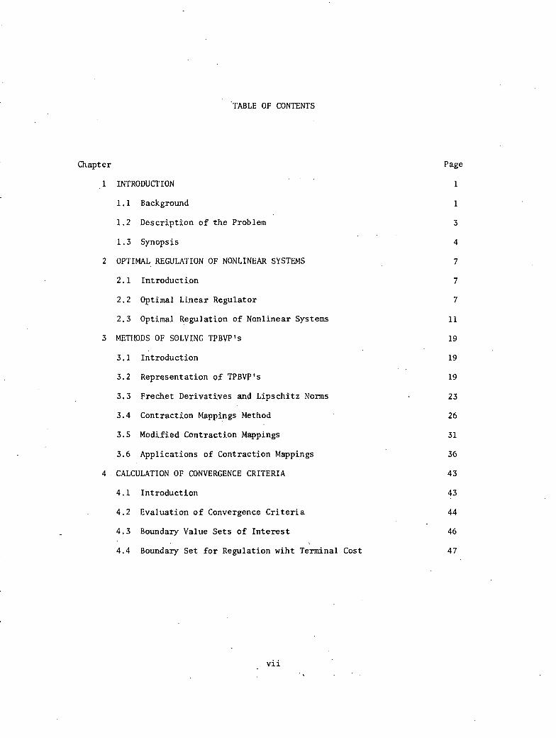
'TABLE OF CONTENTS
Chapter Page
1 INTRODUCTION 1
1.1 Background 1
1.2 Description of the Problem 3
1.3 Synopsis 4
2 OPTIMAL REGULATION OF NONLINEAR SYSTEMS 7
2.1 Introduction 7
2.2 Optimal Linear Regulator 7
2.3 Optimal Regulation of Nonlinear Systems 11
3 METHODS OF SOLVING TPBVP's 19
3.1 Introduction 19
3.2 Representation of TPBVP's 19
3.3 Frechet Derivatives and Lipschitz Norms 23
3.4 Contraction Mappings Method 26
3.5 Modified Contraction Mappings 31
3.6 Applications of Contraction Mappings 36
4 CALCULATION OF CONVERGENCE CRITERIA 43
4.1 Introduction 43
4.2 Evaluation of Convergence Criteria 44
4.3 Boundary Value Sets of Interest 46
4.4 Boundary Set for Regulation wiht Terminal Cost 47
vii
Page
4.5 Boundary Set for Regulation with No Terminal Cost 54
4.6 Application of Similarity Transformation 56
4.7 Approximate Technique 66
5 CONTROLLABILITY FOR NONLINEAR SYSTEMS 71
5.1 Introduction 71
5.2 Controllability for Linear Systems 71
5.3 Nonlinear Controllability 75
5.4 Evaluation of Controllability Convergence Parameters 84
6 NUMERICAL EXAMPLES 91
6.1 Introduction 91
6.2 Van der Pol's Equation 92
6.3 Null Controllability with Bounded Control 102
6.4 Controllability of Satellite Pitch Motion 109
7 PRELIMINARY STUDY ON THE DYNAMICS OF DRUG USAGE WITHIN A COMMUNITY 119
7.1 Introduction 119
7.2 Development of a Dynamic Model 120
7.3 Optimal Regulation of the Nonlinear System 130
8 SUMMARY, CONTRIBUTIONS AND RECOMMENDATIONS 141
8.1 Summary 141
8.2 Contributions 143
8.3 Recommendations 143
Appendix 145
' A Description of Contraction Mappings Computer Algorithm 145
Bibliography 173
viii
LIST OF FIGURES
Figure
6.1 The sphere
6.2 The sphere
Page
96
98
6.3 Control iterations 101
6.4 Comparison of performance for contraction mappings and modified 102
contraction mappings
6.5 The sphere g(yo,r)
6.6 The sphere (ycl,r) for T =
6.7 The sphere g(yo,r) for T = Tr/2
6.8 State and control history
7.1 Levels of drug usage
7.2 Feedback structure of drug usage
7.3 Availability of Potential Users multiplier
7.4 Availability of Drug Users multiplier
7.5 Effect of education on addiction growth rate
7.6 Police effectiveness
7.7 Availability of Addicts multiplier
7.8 Police effectiveness
7.9 Effect of education on addiction growth rate
7.10 The function y0(t) for T = 12 months
7.11 Addicts, Police, and Education for T = 12 months
7.12 The function y0(t) for T = 48 months
7.13 Addicts, Police, and Education for T = 48 months
ix
106
112
115
117
121
121
124
125
126
127
128
134
134
135
137
138
139
CHAPTER t
INTRODUCTION
1.1. Background
Optimal control theory has experienced an increasing growth of interest in
the past two decades. Initially motivated by the aerospace effort, optimal control
theory is now involved in many aspects of general systems engineering. Applica-
tions range from chemical process control to attempts at managerial and economic
planning.
One of the most important and most widely treated problems to date in
optimal control theory is the so-called "Linear Regulator Problem". Historically,
this problem arose in Wiener's work concerning stationary time series and linear
filtering and prediction [W1]. Under the name 'Minimum Integral Squared Error",
development of this problem was continued through the 1950's by Newton [N1],
Booten [B3],and Zadeh [Z1]. Finally utilizing the techniques of modern control
theory, Kalman [K1] presented important new aspects of the problem.
The prominence of this problem is' due to two primary factors. First, the
problem provides a strong link between the classical methods of analytic feedback
system design via frequency domain methods and the more recent variational approach
favoring analysis in the time domain [K4], [W2]. Secondly, the problem allows the
determination of optimal controls in closed form with mathematical ease. (For
general development and presentation of the problem, see Athans and Falb' [A1] and
Lee and Markus [L1]). Finally, a pragmatic motivation for considering the
problem is the ease with which the quadratic cost criteria can be interpreted
1
z
physically. Consequently, optimal linear regulation has been extensively
applied to various systems. For example, the theory has found widespread
applications in the area of automatic flight control systems. Much of this
work is based on the significant efforts of Rynaski [R4], [R5]. Other examples
of optimal linear regulation are contained in Dyer and McReynolds [D2].
However, few systems can adequately be described by a linear dynamic model.
In particular, increasing effort is now being devoted to the development of
models representing systems as varied and as complex as urban areas, natural
resource depletion, management of R and D efforts, and drug usage within a
community. These models are primarily due to the efforts of Forrester [F3,
F4,F5,F6] and Roberts [R2]. Along with many engineering systems, these systems
contain inherent nonlinearities which must be included in any meaningful study.
In contrast to linear systems, the regulation of nonlinear dynamical systems
has received limited attention, most of a specialized nature. The primary reason
for this seems to lie in the fact that nonlinear optimal control problems can
rarely be solved analytically or, more specifically, in feedback form as for
linear regulators. As a result, one must often resort to iterative numerical
techniques for the determination of the optimizing solutions. Consequently, much
of the analysis regarding regulation of nonlinear systems concerns techniques for
determining suboptimal feedback controllers. (See for example [D1], [G2], [L3],
[P1], [S2], [J1], [F8], and [B5]). Most of these approaches involve the modeling
of the nonlinear system as a linear system in some manner. A somewhat different
approach, not suboptimal, is taken by Brunovsky [B4] and Lukes [L4]. Both of
these treatments are closely related to the basic hypothesis that the system be
stabilizable [L1]. Under the assumption of complete controllability, Brunovsky
approached the problem via Lyapunov functions. Lukes requires the system be
2
stabilizable and then uses Lyapunov-like theory to obtain results for feedback
controllers.
The direction of these various approaches is primarily generated by the
desire for a feedback controller. However, there is a second, more esoteric
reason, and that is the desire for general results. Unfortunately, the undis-
cerning application of an algorithm often limits insight into the underlying
structure of the problem being considered. This loss of general information is
often due to the fact that practical convergence criteria are few for most of
the iterative methods used in the solution of optimal control problems. Theoreti-
cal aspects of these criteria have been investigated by numerous applied mathe-
maticians (see Kantorovich [K4] and Collatz [C2]). The Russian Kantorovich [K4]
was one of the first to develop and unify the mathematical theory of iterative
methods. Using the power of functional analysis methods, he presented conver-
gence results for such basic iterative schemes as contraction mappings and
Newton's method. These basic results have been considerably broadened, modernized,
and made practical by the efforts of Falb and de Jong [F1]. In their book, they
present the derivation of general convergence criteria for the application of
various successive approximation methods to the solution of optimal control
problems.
1.2. Description of tha Problem
The primary goal of this research is the consideration of the theoretical
and applied aspects of successive approximation techniques for the solution of
optimal nonlinear regulator problems. Application of the Pontryagin principle
to the posed optimization problem results in necessary conditions for optimality
in the form of a two point boundary value problem (IPBVP). Hence, the central
3
theme of this study shall be the application of successive approximation methods
to the solution of nonlinear TPBVP's which arise from optimal nonlinear regulation.
The basic approach to be used is to represent the TPBVP by an operator equation
and then apply functional analytic results in the iterative solution of operator
equations.
In particular, we shall investigate the contraction mappings method and the
modified contraction mappings method. We have as our first objective the trans-
lation and application of the general convergence theorems to those operators
originating in the optimal regulation of a nonlinear system. A second objective
is the development of techniques to facilitate the evaluation of the convergence
criteria. Finally, example problems will be solved to demonstrate the usefulness
of the theory.
1.3. Synopsis
A brief summary of the dissertation is as follows: In Chapter 2, the optimal
regulation of dynamical systems is introduced. In particular, we discuss the
reduction of optimization problems to two point boundary value problems by means
of Pontryagin's principle. Results are derived for optimal regulation of linear
dynamical systems (Section 2.2) and several classes of nonlinear systems (Sec-
tion 2.3). Optimal system regulation is considered for both unconstrained and
bounded controls. In Chapter 3, methods of solving two point boundary value
problems are presented. In particular, the integral equation representation
of two point boundary value problems is introduced (Section 3.2). The book by
Falb and de Jong [Fl] was used as.the main reference for this chapter. The
integral representation makes it possible to consider the solution of a two
point boundary value problem as the solution of a corresponding operator equation.
4
A review of Lipschitz norms and derivative norms for the integral operator is
presented (Section 3.3) and the methods of contraction mappings (Section 3.4)
and modified contraction mappings (Section 3.5) are introduced. Convergence
theorems for both methods are presented. Chapter 3 concludes with the application
of contraction mappings to the solution of two point boundary value problems
arising in Chapter 2 and the derivation of translated convergence theorems.
Chapter 4 is devoted to a rather detailed investigation into the calculation
of the theoretical convergence criteria. Upper bounds are presented for the
Lipschitz norm and derivative norm (Section 4.2) and various techniques for
evaluating these bounds are introduced.
structured matrices (Sections
4.6) are considered. The use
provides considerable insight
contained within the integral
4.4, 4.5)
In particular, the use of simply
and similarity transformations (Section
of partitioned matrices in these developments
into the generic structure of the
representation. In Chapter S the
Green's matrices
issue of con-
trollability for nonlinear systems is considered. Specifically, it is shown
that controllability for linear systems (Section 5.2) and nonlinear systems
(Section 5.3) may be studied via the integral representation and contraction
mappings. In Chapter 6 we present numerical examples to illustrate the theoreti-
cal and practical application of contraction mappings to the regulation and
control of nonlinear systems. In Chapter 7, a dynamic model is developed for
a socio-economic system and contraction mappings is used to investigate the
optimal regulation of this nonlinear system. Finally, in Chapter 8, we summarize
our results and indicate directions in which future research may be done. We
conclude with an appendix which gives the actual computer program (written in
the FORTRAN language) which was used in the application of contraction mappings
to the problem discussed in Chapter 7.

Page intentionally left blank
CHAPTER 2
OPTIMAL REGULATION OF DYNAMICAL SYSTEMS
2.1. Introduction
An optimal control problem is a composite concept consisting of four basic
elements: (1) a dynamical system, (2) a set of initial states and a set of final
states, (3) a set of admissible controls, and (4) a cost functional to be minimized.
The problem consists of finding the admissible control which transfers the state
of the dynamical system from the set of initial states to the set of final states
and, in so doing, minimizes the cost functional. In this chapter we discuss the
optimal regulation of nonlinear systems and the reduction of the optimization
problem to a TPBVP by means of Pontryagin's principle.
2.2. Optimal Linear Regulator
As a preface to the nonlinear system analysis, we shall present the basic
results for the optimal linear regulator. (For a very thorough treatment of this
problem see Kleinman [K4]).
Definition 2.2.1. Linear Dynamical System
A linear dynamical system is characterized by the following elements:
(1) A state vector x of dimension n
(2) A control input vector u of dimension r
(3) A linear differential equation which describes the evolution of the
system in time, i.e.,
i(t) = A(t) x(t) + B(t) u(t)
where A(t) is an nxn matrix and B(t) is an nxr matrix.
2.2.2
•
1
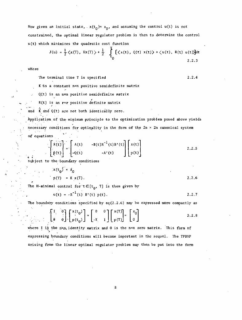
Now given an initial state, x(t0)= x0, and assuming the control u(t) is not
constrained, the optimal linear regulator problem is then to determine the control
u(t) which minimizes the quadratic cost function
J(u) = 12-<x(T), Kx(T)> + kx(t), Q(t) x(t)> + <u(t), R(t) u(t)Adt
t02 . 2 . 3
wHere
The terminal time T is specified 2.2.4
K a constant nxn positive semidefinite matrix
Q(t) is an nxn positive semidefinite matrix
R(t) is an rxr positive definite matrix
and 1( and Q(t) are not both identicålly zero.
Applicatipn of the. minimum principle to the optimization problem posed above yields
necessary conditions for optiikality in the form of the 2n x 2n canonical system
a •
G
stkbject to the 'boundary conditions
,x(t0)= XO
p(T) = K x(T).
The H-minimal control for 't E[to, T] is then given by
u(t) = -R-1(t) B'(t) p(t).
of equations
I[kcty . A(t) -B(t)12-1(t)B'(t) x(t)
(t) . -Q(t) -A' (t) p(t)2.2.5
2.2.6
2 .2 . 7
The boundary tonditions specified by eq(2.2.6) may be expressed more compactly as
[I
.oi r x(toi+ r ormi= r x01cd,Lp(toi L-K I p (T) 1_ 0
2. 2 . 8
where I ijS the nxii, identity matrix and 0 is the nxn zero matrix. This form of- -,
expressing boundary conditions will become important in the sequel. The TPBVP
arising from the linear optimal regulator problem may then be put into the form
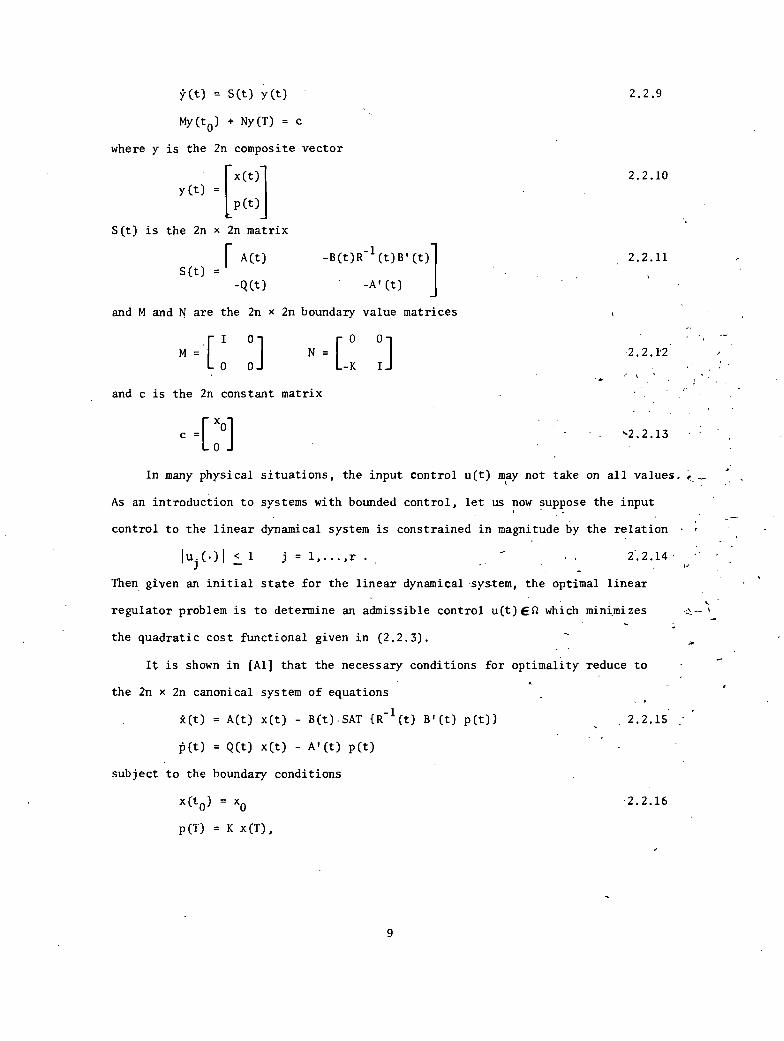
0 0
y(t) = S(t) y(t)
My(to) + Ny(T) = c
where y is the 2n composite vector
[x(t)]y (t) =
p(t)
S(t) is the 2n x 2n matrix
F A(t) -1-B(t)R (t)B'(t)
S(t) =-Q(t) -A'(t)
and M and N are the 2n x 2n boundary value matrices
I 0 ] [ 0 0N =
-K 1Jand c is the 2n constant matrix
xc =
0
0
2.2.9
2.2.10
2.2.11
2.2.12'
•
In many physical situations, the input control u(t) may not take on all values.
As an introduction to systems with bounded control, let us now suppose the input
control to the linear dynamical system is constrained in magnitude by the relation - •
< 1 j = 1,...,r . 2.2.14'
Then given an initial state for the linear dynamical system, the optimal linear
regulator problem is to determine an admissible control u(t)4E0 which minimizes
the quadratic cost functional given in (2.2.3).
It is shown in [A1] that the necessary conditions for optimality reduce to
the 2n x 2n canonical system of equations
i(t) = A(t) x(t) - B(t) SAT {R-1(t) B'(t) p(t)}
= Q(t) x(t) - A'(t) p(t)
subject to the boundary conditions
x(t0) = x0
p(T) = K x(T),
9
2.2.15 2
2.2.16
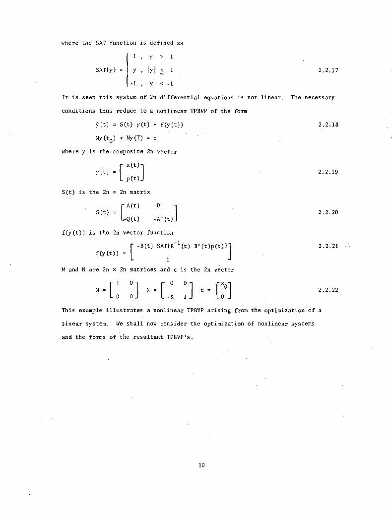
where the SAT function is defined as
1 , y > 1
SAT{y} = Y IYI < 1 2.2.17
-1 , y < -1
It is seen this system of 2n differential equations is not linear. The necessary
conditions thus reduce to a nonlinear TPBVP of the form
ý(t) = S(t) y(t) + f(y(t)) 2.2.18
My(t0) + Ny(T) = c
where y is the composite 2n vector
y(t) = I x(t)1L p(t)i
S(t) is the 2n x 2n matrix
S(t) A(t) 0
[-Q(t) 40(t)i
f(y(t)) is the 2n vector function
f(y(t)) =[ -B(t) SAM
-1 (t) P(t)p(t)}]
0
M and N are 2n x 2n matrices and c is the 2n vector
M =[ I 0
N[ 0 ]
c0
[x
0 0 -K I 0
2.2.19
2.2.20
2.2.21 -
2.2.22
This example illustrates a nonlinear TPBVP arising from the optimization of a
linear system. We shall now consider the optimization of nonlinear systems
and the forms of the resultant TPBVP's.
10
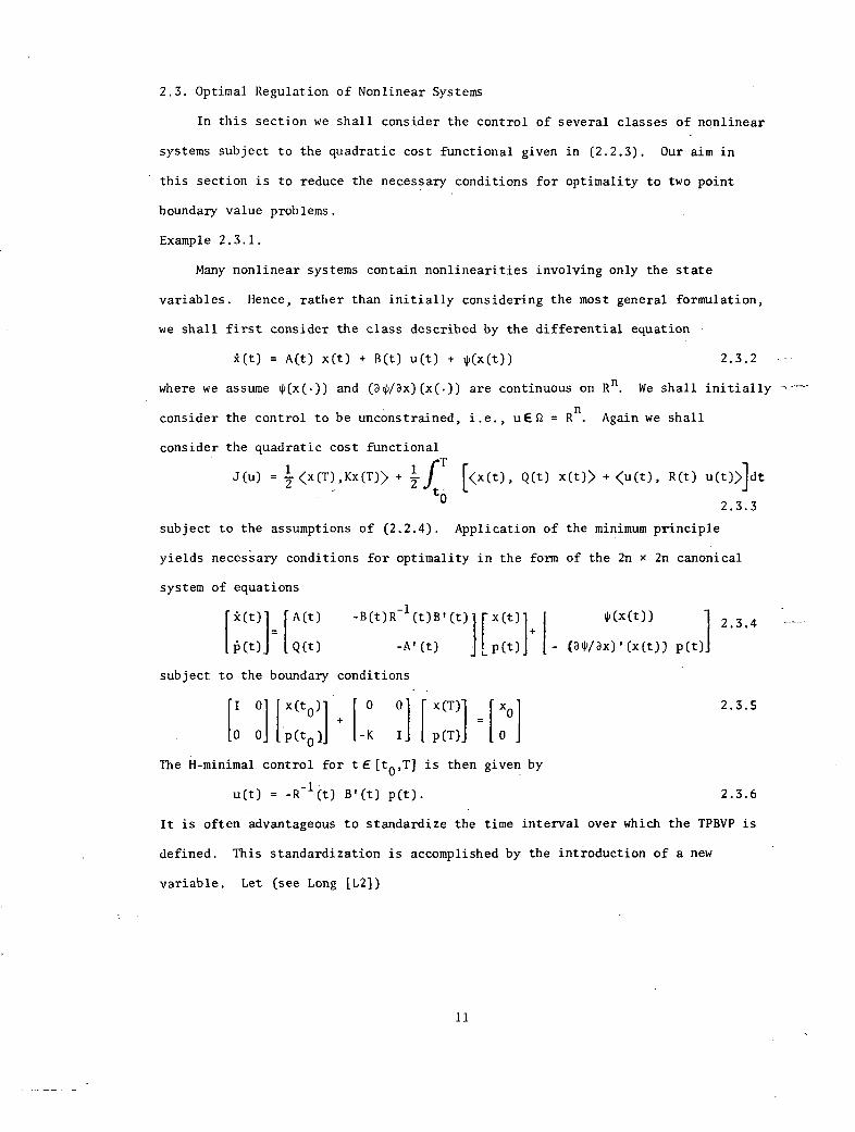
2.3. Optimal Regulation of Nonlinear Systems
In this section we shall consider the control of several classes of nonlinear
systems subject to the quadratic cost functional given in (2.2.3). Our aim in
this section is to reduce the necessary conditions for optimality to two point
boundary value problems.
Example 2.3.1.
Many nonlinear systems contain nonlinearities involving only the state
variables. Hence, rather than initially considering the most general formulation,
we shall first consider the class described by the differential equation
i(t) = A(t) x(t) + B(t) u(t) + Ip(x(t)) 2.3.2
where we assume *(x(.)) and (311)/Dx)(x(.)) are continuous on Rn. We shall initially
consider the control to be unconstrained, i.e., uE St = R. Again we shall
consider the quadratic cost functional
1J(u) = 7. <x(T),Kx(T)› + [<x(t), Q(t) x(t)› + <u(t), R(t) u(t)ddt-2f
02.3 3
subject to the assumptions of (2.2.4). Application of the minimum principle
yields necessary conditions for optimality in the form of the 2n x 2n canonical
system of equations
[kW]. A(t) -B(t)R-1(t)P(t)iix(t) ip(x(t))
2.3.4
[P(t)] Q(t) -A'(t) [1)(01 I- (310x)'(x(t)) P(t)]
subject to the boundary conditions
I 0 lx(to)1
0 0 p(t0)]
0 0 x(T) x0
-K I
{
p(T)
.
[ 0
2.3.5
The H-minimal control for t E [to,T] is then given by
u(t) = -R-1(t) B'(t) p(t). 2.3.6
It is often advantageous to standardize the time interval over which the TPBVP is
defined. This standardization is accomplished by the introduction of a new
variable. Let (see Long [L2])
11
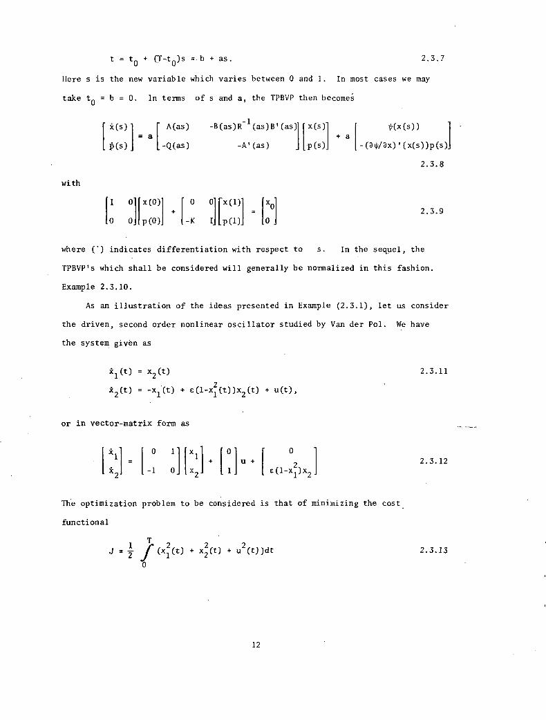
t = t0
+ ('F-t0 )s ..b + as. 2.3.7
Here s is the new variable which varies between 0 and 1. In most cases we may
take t0
= b = O. In terms of s and a, the TPBVP then becomei
with
i(s) A(as) -B(as)R-1(as)B'(as) x(s)
= ap(s) J -Q(as) -A' (as) p(s)
I 01 [ x (0) 0 01 rx (1)1 xd
0 0 p(0) d[p(1)] 10
+ aip(x(s))
-(4/3x)'(x(s))p(s)1
2.3.8
2.3.9
where (*) indicates differentiation with respect to s. In the sequel, the
TPBVP's which shall be considered will generally be normalized in this fashion.
Example 2.3.10.
As an illustration of the ideas presented in Example (2.3.1), let us consider
the driven, second order nonlinear oscillator studied by Van der Pol. We have
the system given as
*1(t) = x2(t) 2.3.11
)12(t) = -x
1(t) + e (1-x
12 (t))x
2(t) + u(t) ,
or in vector-matrix form as
k1
0 1 Exil 4. [01 u 4. 02.3.12
21 -1 1 x2 t [ c(1-x2)x 2 [1
The optimization problem to be considered is that of minimizing the cost
functional
T2
J = ¡
(x2 (t) + x (t) + u
2(t))dt
12.3.13
0
12
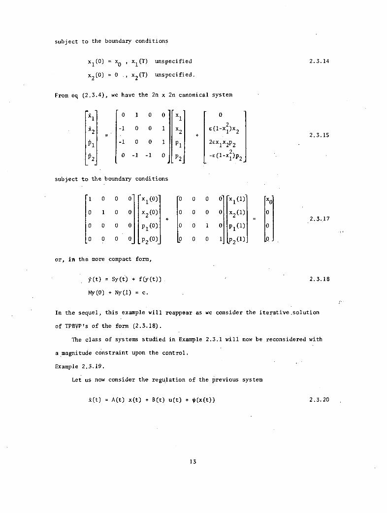
subject to the boundary conditions
x1(0) = x0 , xl(T) unspecified
x2(0) = 0 ., x2(T) unspecified.
2.3.14
From eq (2.3.4), we have the 2n x 2n canonical system
10100 x
10
2-1 0 0 1 x
2e(1-x1
2 )x2
2.3.15
pl-1 0 0 1
P12ex
1x2p2
P20 -1 -1 0
P22
-e(1-xdp2
subject to the boundary conditions
1 0 0 0 x1(0) o o x1(1) xo
0 1 0 0 x2(0) o o 0 ox2(1)
02.3.17
0000 p1(0) o o 1 oP1(1)
0 0 0 0 p2 (0)
_o o
P2(1)
or, in the more compact form,
Y(t) = Sy(t) + f(y(t)) 2.3.18
Ny(1) = c.
In the sequel, this example will reappear as we consider the iterative.solution
of TPBVP's of the form (2.3.18).
The class of systems studied in Example 2.3.1 will now be reconsidered with
amagnitude constraint upon the control.
Example 2.3.19.
Let us now consider the regulation of the previous system
i(t) = A(t) x(t) + B(t) u(t) + *(x(t)) 2.3.20
13
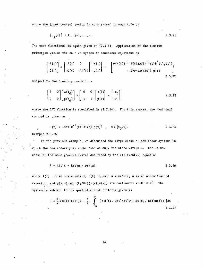
where the input control vector is constrained in magnitude by
111.(.)1 < 1 , j=1,...,r.
The cost functional is again given by (2.3.3). Application of the minimum
principle yields the 2n x 2n system of canonical equations as
2.3.21
r ),(t)] { A(t) 0 x(t) ip(x(t)) - B(t)SAT{R-1(t)B'Wp(t)}
[ -Q(t) -A'(t) p(t) - (Waxix(t)) p(t)
2.3.22
subject to the boundary conditions
I Olixx(t0) 1 0 0 x (T)1
0 0 p (to) -K I p (T).1 OxF 2.3.23
where the SAT function is specified in (2.2.16). For this system, the H-minimal
control is given as
u(t) = -SAT{R-1(t) B'(t) p(t)} , te[to,T]. 2.3.24
Example 2.3.25
In the previous example, we discussed the large class of nonlinear systems in
which the nonlinearity is a function of only the state variable. Let us now
consider the more general system described by the differential equation
ic = A(t)x + B(t)u + gx,u) 2.3.26
where A(t) is an n x n matrix, B(t) is an n x r matrix, u is an unconstrained
r-vector, and ti(x,u) and (4/3x)(x(.),u(.)) are continuous in Rn x Rn. The
system is subject to the quadratic cost criteria given as
1J =
2 —<x(T),Kx(T)> + 7 f [<x(t), Q(t)x(t)> +<u(t), R(t)u(t)>]dt
T
to2.3.27
14
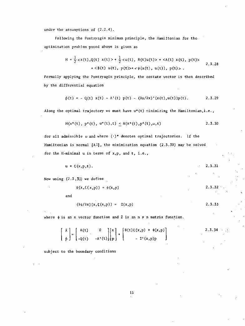
under the assumptions of (2.2.4).
Following the Pontryagin minimum principle, the Hamiltonian for the-
optimization problem posed above is given as
1H = T<x(t),Q(t) x(t)> +
1 <u(t), R(t)u(t)> + <A(t) x(t), p(t)>
2.3.28+ <B(t) u(t), p(t)>+ <--Ip(x(t), u(t)), p(t)> .
Formally applying the Pontryagin principle, the costate vector is then described
by the differential equation
p(t) = - Q(t) x(t) - A'(t) p(t) - (91p/ax)'(x(t),u(t))p(t). 2.3.29
Along the optimal trajectory we must have u*(t) minimizing the Hamiltonian,i.e.,
H(x*(t), p*(t), u*(t),t) < H(x*(t),p*(t),w,t) 2.3.30
for all admissible w and where (.)* denotes optimal trajectories. If the
Hamiltonian is normal [A1], the minimization equation (2.3.30) may be solved
for the H-minimal u in terms of x,p, and t, i.e.,
u = C(x,p,t). - 2.3.31
Now using (2.3.31) we define
xi(x,“x,P)) = gx,p) 2.3.32
and
(30/3x)(x,“x,p)) = Z(x,p) 2.3.33
where 0 is an n vector function and Z is an n x n matrix function.
k A(t) 0 x [B(t)“x,p) + 0(x,p)1 2.3.34
pi -Q(t) -A' (t) p - Z' (x,p)p
subject to the boundary conditions
15

I 0 x(t0)1 0 0 [ x(T)
[ 0 0 [[ p (to) -K I II p(T)
These results may be applied to various forms of gx,p). In the following
example we consider one such form.
Example 2.3.36
Consider the system described by
2.3.35
A = A(t)x + B(t)u + D(x)u 2.3.36
where A(t) is an n x n matrix, B(t) is an n x r matrix, D(x) is an n x r matrix,
jDii(x) and (3D
i/3x
k )(x(.)) are continuous in R
n , and u(•) is an unconstrained
r vector. Consider system (2.3.36) subject to the cost functional (2.3.27) and
tht initial condition x(t0) = xo.
Define the vector function “x,p,t) to contain the elements
yx,p,t) = lp, - (BD/axi)(x) R-1(t)W(t) + D'(x)h*
and define the matrix c(x,t) as
C(x,t) =-B(t) Oct) (t) - .D(x) 11-1(t)[}3t(t) + (x)]. '
2.3.37
2.3.38 =-
Usi,ng the results of Example 2.3.25 and (2.3.37), (2.3.38), the 2n x 2n canonical
sys,tem of equations is given as
A A(t) -13(t)R-1(t)13'(t) x C(x,t)p
p -czct) -A(t) J I p E(x,p,t)
I I 01x(tn)] 0 0 x(T) x0
0 0.11p (to) [-K Ill p(T) =[ 0
The various two point boundary value problems presented in the previous
16
2.3.39
2.3.40

examples can very rarely be solved analytically. Thus we shall investsigate
successive approximation techniques for the solution of TPBVP's in the next
chapter.
17

Page intentionally left blank
CHAPTER 3
METHODS OF SOLVING TPBVP's
3.1. Introduction
In the analysis of optimal control problems, the necessary conditions for
optimality are often in a form which may be reduced to a TPBVP of the form
y(t) = F(y,t), g(y(0)) + h(y(1)) = c. 3.1.1
In particular, we presented in Chapter 2 various TPBVP's which originate in the
optimal regulation of certain classes of nonlinear systems. We shall now illustrate
that under certain conditions, such TPBVP's may be represented by operator equations
of the form
Y = T(Y). 3.1.2
Then, following the lead of Falb and deJong [F1], we shall investigate the applica-
tion of successive approximation techniques to the iterative solution of these
operator equations.
3.2 Representation of TPBVP's
In this section we consider the (normalized) two point boundary value problem
Y(t) = F(y,t), g(y(0)) + h(y(1)) = c 3.2.1
where G, g, and h are vector valued functions and c is an element of R . We
shall first review some results relating to the development of equivalent integral
equation representations of the TPBVP(3.2.1). Most results in this section.
19
come from Falb and de Jong [F1]. Since linear TPBVP's will play an important
role in the integral equation representations, we begin our discussion with a
consideration of linear TPBVP's.
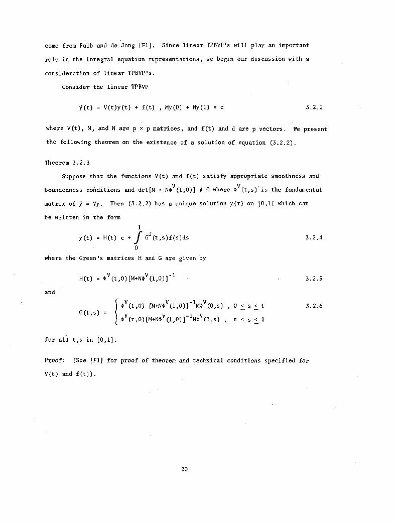
Consider the linear TPBVP
y(t) = V(t)y(t) + f(t) , My(0) + Ny(1) = c 3.2.2
where V(t), M, and N are p x p matrices, and f(t) and d are p vectors. We present
the following theorem on the existence of a solution of equation (3.2.2).
Theorem 3.2.3
Suppose that the functions V(t) and f(t) satisfy appropriate smoothness and
boundedness conditions and det[M + N4Y(1,0)] # 0 where 4Y(t,$) is the fundamental
matrix of jr = Vy. Then (3.2.2) has a unique solution y(t) on [0,1] which can
be written in the form
1y(t) = H(t) c + .ir Gj(t,$)f(s)ds
0
where the Green's matrices H and G are given by
and
H(t) =v(t,0)[M+N(DV(1,0)]
-1
G(t,$) =
for all t,s in [0,1].
4,11(t,0) [M+N4)v(1,0)] 1M4Y(0,$) , 0 < s < t
-4)11(t,0)[M+N4Y(1,0)]_ 1 40V(1,$) , t < s < 1
3.2.4
3.2.5
3.2.6
Proof: (See [F1] for proof of theorem and technical conditions specified for
V(t) and f(t)).
20
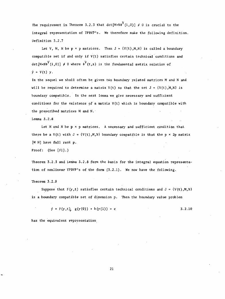
The requirement in Theorem 3.2.3 that det[M+NOV(1,0)] / 0 is crucial to the
integral representation of TPBVP's. We therefore make the following definition.
Definition 3.2.7
Let V, M, N be p x p matrices. Then J = {V(t),M,N} is called a boundary
compatible set if and only if V(t) satisfies certain technical conditions and
det[M+NOV(1,0)] / 0 where OV(t,$) is the fundamental matrix solution of
= V(t) y.
In the sequel we shall often be given two boundary related matrices M and N and
will be required to determine a matrix V(t) so that the set J = fV(t),M,N1 is
boundary compatible. In the next lemma we give necessary and sufficient
conditions for the existence of a matrix V(t) which is boundary compatible with
the prescribed matrices M and N.
Lemma 3.2.8
Let M and N be p x p matrices. A necessary and sufficient condition that
there be a V(t) with J = {V(t),M,N} boundary compatible is that the p x 2p matrix
N] have full rank
Proof: (See [F1].)
p.
Theorem 3.2.3 and Lemma 3.2.8 form the basis for the integral equation representa-
tion of nonlinear TPBVP's of the form ,(3.2.1). We now have the following.
Theorem 3.2.9
Suppose that F(y,t) satisfies certain technical conditions and J = {V(t),M,N}
is a boundary compatible set of dimension p. Then the boundary value problem
= F(y,t), g(y(0)) + h(y(1)) = c 3.2.10
has the equivalent representation
21
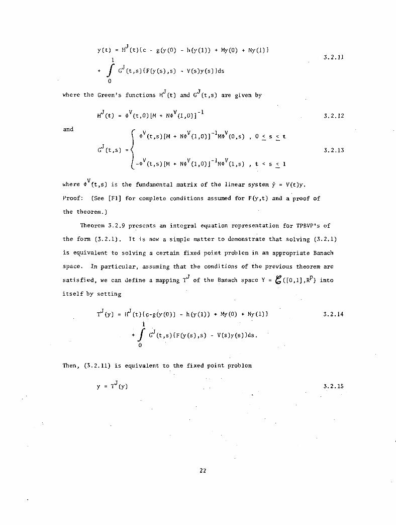
y(t) = Hj(t){c - g(y(0) - h(y(1)) + My(0) + Ny(1)}
1
f Gj(t,$)1F(y(s),$) - V(s)y(s)}ds
0
where the Green's functions Hj(t) and G (t,$) are given by
and
Hj(t) = (t,0)[M + Nod/(1,0)]-1
v(t,$)[M + NO
v(1,0)] 1MOV(0,$) ,0<s< t
-(01(t,$)[M + NOV(1,0)] 1NOV(1,$) , t< s < 1
where 4, (t,$) is the fundamental matrix of the linear system jr = V(t)y.
3.2.11
3.2.12
3.2.13
Proof: (See [Fl] for complete conditions assumed for F(y,t) and a proof of
the theorem.)
Theorem 3.2.9 presents an integral equation representation for TPBVP's of
the form (3.2.1). It is now a simple matter to demonstrate that solving (3.2.1)
is equivalent to solving a certain fixed point problem in an appropriate Banach
space. In particular, assuming that the conditions of the previous theorem are
satisfied, we can define a mapping Tj of the Banach space Y = t;([0,1],e) into
itself by setting
Tj(y) = Hj(t){c-g(y(0)) - h(y(1)) + My(0) + Ny(1)}
1
+f Gj(t,$){F(y(s),$) - V(s)y(s)lds.
0
Then, (3.2.11) is equivalent to the fixed point problem
Y = Tj(Y)
22
3.2.14
3.2.15
on e([0,1],RP). The operator equation (3.2.14) can now be solved by successive
approximation iterative techniques as presented by Kantorovich [K4] and particu-
larly Falb and de Jong [F1].
3.3. Frechet Derivatives and Lipschitz Norms
In the discussion of successive approximation iterative techniques, we shall
require an expression for the Frechet derivative or Lipschitz norm of the operator
T . In this section we shall present a brief treatment of these concepts. (Again,
many of these basic results are from Falb [F1].) Let us begin with the following
definition.
Definition 3.3.1.
Let Y be a Banach space with as norm. Let S2 be a closed subset of Y
and let T map Y into Y. The Lipschitz norm of T on 0, in symbols: IT O cl , is
given by
T I = us,uvP St T(u) - T(v)Il/ 11 u-v 111. 3.3.2
If T is Frechet differentiable on 0, then derivative norm of T on 0, in symbols:
OTO'0
is given by
II (Ty ) I f
We shall now compute expressions for (Ty )' and (T
yj)" . We have
and
(r YJ),(u) = Hj(t)(EM-(ag/3y)(y(0))]u(0) + [N-(311/3y)(y(1))]u(1)}
1
f Gj(t,$){(3F/ay)(y(s)) - V(s)}u(s)ds0
23
3.3. 3
3.3.4
(Tj)"(u,v) = Hj(t) E [ (a/ayi) (-ag/ay)] (y(0))ui (0)v (0))
E [(a/ayi) (-ah/ay)] (y (1))ui (1)v(1)
i=1
Gj(t,$) j E [ (a/ayi) (aF/3y)] (y(s))ui (s)v(s) ds 3.3.5
i=1
provided the indicated partial derivatives exist. When evaluating convergence
criteria, we shall require estimates, say for example of the norm of the operator
(T )' . There are of course several expressions for calculating or estimating
II (1. )111 . Since the more accurate expressions are difficult to evaluate in
practice, we shall present a coarse estimate that is more amenable to future
applications . We recall first of all that if v(•)E ((Om , RP), then
liv(.) 11 = sup sup Iv. (t) l 3.3.6i c P te [0,1] 1
is the norm of v(• ) where P = {1, ... ,p} and vi (•) is the ith component of v(• ).
Noting that li(T j) '11 = sup { 11 (Tuj) 'u 111 and letting Hj(t) = [ijii (t)] ,Y Hull <1
G (t,$) = [G. . (t,$)] , M = [injk] , N = [njk], V (s) = [vjk (s)] , we have as a coarse13
estimate
ff(Tjj) = sup li(T j) 'u II 1,Hull <1 Y
P P1i
1< sup sup 1 T` (1H . (t) a ( E {lmjk - (agj/ayk) (y (0)) 1i E P t 4—d
j
j=1 k=1
+ l n jk - (ah./ayk )(Y(1))1 1)j
24
3.3.7

P 1
+ ( 13
(t,$)Ids).( sup I :E: l(aF./aYk j )(Y(s),$) - v k (s)19 1
j=1 0 s k=1
Expression (3.3.7),will become quite important in the sequel. One of our primary
objectives shall be determining techniques for easily estimating this expression.
In some cases, the smoothness conditions required to obtain Frechet deriva-
tives are too strong. As an example, we have the nonlinearity containing the
SAT function in equation (2.2.15). This fact does not imply that successive
approximating techniques may not be applied to the iterative solution of the
operator equation. It simply means we have lost one method of evaluating
convergence criteria. Hence, under somewhat weaker smoothness conditions, we
shall compute the Lipschitz norm of the operator Tj(y).
We have the following result from Falb [F1].
Lemma 3.3.8
Let S be a bounded open set in e([0,1],RP) and let D be an open set in
RP containing the range of S. Suppose that (i) K(t,y,$) is a map of
[0,1] x D x [0,1] into D which satisfies certain technical conditions, and (ii)1
there is an integrable function m(t,$) of s with sup fm(t,$)ds = u < co sucht o
that I K(t,y,$) II < m(t,$) and OK(t,y1,$) - K(t,y2,$)I1 <411(t,$) Ry1-y2 on
[0,1] x D x [0,1]. Then the mapping T given by
1
T(u) (t) = f K(t,u(s),$)ds
0
maps e([0,1],e) into g([0,1],e) and the Lipschitz norm, IITQ s, satisfies
RTfi s < p. 3. 3. 9
Proof: (See [F1] for proof of theorem and specific conditions on K.)
25
Corrollary 3.3.10
Suppose that the function
K(t,y,$) = Gj(t,$){F(y,$) - V(s)y}
sattsfies the conditions of Lemma 3.3.8 and that
Let
Then
This
0 g(y1) - g(y2) il < 111 11 yl-y2 1t and 0 h(y1)-h(y2) II < P2 q y1-y2 II 3.3.11
a = max {p, II Hj(•) II 1.11, li Hj(•) II p2,0 Hj(•)M 0 , b Hj(•)N II }. 3.3.12
L. a 3.3.13
result will prove useful in particular when investigating regulators with
bounded input controls.
3.4. Contraction,Mappings Method
Contraction mappings (or Picard's method, [P2]) is well known in the mathemat-
ical literature and has long been a standard approach for proving existence and
uniqueness properties for ordinary differential equations. (See for example
Coddington and Levinson [C1], specifically Section 1.3 entitled "The Method of
Successive Approximations.") To formalize our discussion of this technique, let
us begin with the following definition.
Definition 3.4.1
Let Y be a topological space and let T map Y into itself. Let y0 be
an element of Y. The sequence {yn(•)} generated by the algorithm
yn+1 = T(yn) n = 0,1,2,... 3.4.2
is called a contraction mapping or CM sequence for T based on yo.
The following theorem is central to our future discussions concerning the
contraction mappings method.
26
Theorem 3.4.3
Let Y be a Banach space and let Š = g(yo,r) be the closed sphere in Y with
center yo and radius r. Let T map Y into Y and suppose that (i) T is defined
on kyo,r), and (ii) there are real numbers n and a with n >' 0 and 0 < a < 1
such that
y1 y0 " < n11 T
S < a < 1 or ITis < a < 1
1rl < r1-a —
3.4.4
3.4.5
3.4.6
where yl = T(y0). Then the CM sequence {yrn} for T based on y0 converges to the
unique fixed point y* of T in S and the rate of convergence is given by
y* yn < yn yn_1 < laa H y1 y0 II • 3. 4. 7
Proof: (See [F ]).
Let us now consider the application of this theorem to operator equations of the
form
y(t) = Tj(y)(t) = Hj(t){c-g(y(0))- h(y(1) + My(0) + Ny(1)}3.4.8
1
+ Gj(t,$)(F(y(s),$) - V(s)y(s)}ds
0
where J = {V(t) AN} is a boundary compatible set. Following the contraction
mapping prescription, we select an initial element yo(.) in g([0,1], Rp) and
successively generate a CM sequence (yn(.)) for Tj based on yo(.) by means of
the algorithm
Yn+1 = Tj(Yn)
27
3.4.9
or equivalently, by
Yn.1(t) = Hj(t){c g(y
n(0)) - h(yn(0)) + M
yn(0) + Nyn(1)}
3.4.10
+ f Gj(t,$){F(yn(s),$) - V(s)yn(s)}ds.
Since we know yn(-) at each successive step, we can write (3.4.10) in the form
yn+1
(t) = Hj(t)cn + f Gj(t,$)fn(s)ds
where
cn = c - g(yn(0)) - h(yn(1)) + Myn(0) + Nyn(1)
and
fn(s) = F(yn(s)) - V(s) yn(s).
3.4.11
3.4.12
3.4.13
Hence, it is seen from (3.4.11) and our results on linear TPBVP (eq. 3.2.4) that
the method of contraction mappings when applied to (3.4.8) essentially amounts
to the successive solution of the linear TPBVP's (3.4.11).
If the partial derivatives of (3.3.) exist, we then have the following.
Theorem 3.4.14.
Let yo(.) be an element of e([0,1],e) and let 8 = 8(y0,r). 5uppose that
(i) J = {V(t),M,n} is a boundary compatible set for which
= F(y(t),t) g(y(0)) + h(y(1)) = c 3.4.15
is differentiable on 8, and (ii) there are real numbers n and a with n > 0 and
0 < a < 1 such that
28
ITj(y0) - y0 H = sup te713 {1Tj(Y0)i(t) - y0,i(t)1} < n 3.4.16i
sup O(Tyj)' } < a 3.4.17
yE g
n < r1-a —- '3.4.18
Then the CM sequence {yn(.)} for the TPBVP based on yo and J converges uniformly
to the unique solution y*(.) of (3.4.15) in S and the rate of convergence is
given by
n
11 *(.) - Yn(*) L 3.4.19
Proof: Simply apply Theorem 3.4.3.
It should be noticed that if the TPBVP of interest is not differentiable,
but a Lipschitz norm can be obtained, then (3.4.17) is simply replaced by
0 TJ < a . 3.4.20
We shall use (3.4.20) in the investigation of optimal regulators with bounded
control.
At this point we shall make a few general comments concerning our representa-
tion of TPBVP's and, in partiuclar, the role of the boundary compatible set,
J = {V,M,N}. From Theorem 3.4.14, we see that the convergence rate factor, a,.
is determined by the Frechet derivative of the operator Tj(y). In particular,
from equation 3.3.6 we have an estimate for this norm.given as
29
H(Tj)'11 (TyJ) iu
a l
ag4 ah.
L .sup sup/7(1 le W) )•(E hm. -(---1-)(37(0))1+In. (y(1))11)Itp t a•-• 13 jk ay
j=1 k=1 3k aYk
1P C OF.\
EIGjij (t,$) cis4" I d R-1-"qs".-17. (s) 1/ 4
s . ay. Jkj=1 0 k=1 k
3.4.21
For convergence purposes we wish to make this quantity as small as possible,
and in this light, we shall discuss the dhoice of J = {V(t), M,N}. A11 of the
TPBVP's obtained in Chapter 2 have linear boundary conditions of the form
Ky(0) + Ly(1) = c. From this we shall clearly choose M and N to equal the
linear boundary conditions of the TPBVP, thus eliminating the first terms in
(3.4.21). We then have the simplified expression
1 ,aF.\' I(ry) ILL__ sup sue I E (f ,„• ,t,$) ds) - (sup Z., (-11 (y(s) , s)-v (s) 3.4.22
iep s av jicj=1 lj k=1
Consideration of this expression allows us to deduce that if yo is a good initial
estimate of the solution, then it is often effective to choose V(s) close to
(aF/9y)(yo(s),$). In fact, for V(s) = (aF/3y)(yo(s),$), the iterative method
is known as the "modified Newton's method." However, a general choice such as
this for the V matrix usually precludes any attempt at calculating or estimating
the term Gj(t,$)Ids , thus preventing an easy estimation of the convergence0
criteria. In the next section we shall consider a technique which is often
useful for evaluating convergence criteria.
30
3.5. Modified Contration Mappings
In some situations, the direct application of the contraction mappings
method does not lead to a convergent sequence of approximations. However,
it is frequently possible to modify T in such a way as to lead to a convergent
sequence of approximations. We consider the following.
Lemma 3.5.1.
Let T and U be maps of Y into Y. Suppose that I - U is invertible and let.
P. be the map of Y into itself given by
P(y) = [I-U]-1[T(y) - U(y)]. 3.5.2
Then y*(.) is a fixed point of T if and only if y*(.) is a fixed point of P.
Proof: (See [F1]).
We shall then consider the selection of an initial approximate solution y0 and
the generation of a sequence {yn} by the algorithm
yn+1 = P(Yn) = [I-U]-1
[T(Yn) "Yn)].
We shall call this algorithm the modified contraction mappings method. It
3.5.3
should be noted that the modified contraction mapping sequence for T based on
y0 and U coincides with the contraction mapping sequence for P based on yo.
Hence we may translate the results on contraction mappings into theorems for
modified contraction mappings. The primary theorem is given as follows.
Theorem 3.5.4.
If U is a linear operator with I-U invertible, if T is Olferentiable on Š,
and if there are real numbers n,a with n > 0 and 0 < a < 1 such that
31
II Y1 - Yo II n
sup { II [I-U]-1 [T(Y)
- U] H < ay E S
1n < r,1-a
then the modified contraction mappings sequence {yn} converges to the unique
fixed point y* of T and g and the rate of convergence is given by
nII Y* Yn L laa Yn Yn-1 11 L 1-
aa Y1 - YO II •
3.5.5
3.5.6
3.5.7
3.5.8
Proof: Apply Theorem 3.4.3.
The importance of these results lies in the fact that they extend the range of
applicability of the contraction mapping method to fixed point problems for
operators T that are not contraction mappings. In other words, the basic
contraction mapping criteria
sup f (T j)' 0 < a < 1yE S
is replaced by the condition that the Frechet derivative satisfies
sup {11 [I-U]-1[T
J)'-U]11 } < a < 1.
y S
A second possibility is to replace the single norm in (3.5.10) by a product
of two norms so that
sup { 0 [I-U] 14 • 0 [(T j) 1-U] 0 1 < a < 1.yEs
3.5.9
3.5.10
3.5.11
This formulation offers the possible advantage of easier evaluation, but also
results-in less sharp convergence conditions.
We shall now specify the form of linear operator U that will be used in
the modified contraction mappings algorithm. The following lemma involves
32
the relation between the operators T and TJ for different boundary compatible
sets J = {V(t),M,N} and J = {W(t),K,L}.
Lemma 3.5.12.
Let J = {V(t),M,N} and J = {14(t),K,L} be boundary compatible sets. Let
F(y,t) be continuous in y for each fixed t and measurable in t for each fixed
with IF(y,t)11< m(t), m(t) integrable. Let r be the linear manifold of
absolutely continuous functions in e:([0,1],R ).
given by
Let UKL
be the operator
UKL(y) (t) = H (t) {-Ky(0) - Ly(1) + My(0) + Ny(1)}
1
1Gj(t,$){W(s)y(s) - V(s)y(s)} ds
0
3.5.13
for y(.) in 8;([0,1],e). Then (i) UKL maps e([0,1],0) into g([0,1],e) andr into r ; (ii) the operator I -UKL has a bounded linear inverse on r with
[I-UL MN ]-1
y = [I-V j]yK
for y in r and
VmN 5
y = Hj(t){-My(0) Ny(1) + Ky(0) + Ly(1)}
+JrG (t,$){V(s)Y(s) - W(s)y(s)}ds
(iii) if y(.) is in e([0,1],RP), then
Tj(Y) = [Tj(Y) - Ulja(Y)]
and (iv) under the differentiability assumptions
J(T
UKL]-1
j)' = [I- • [(T )' - UjL ].
K
Proof: (See [F1]).
33
3.5.14
3.5.15
3.5.16
3.5.17
We shall limit our future discussions to operators U = UKL of the form given
by (3.5.13). It then follows from Lemma 3.5.12 that the modified contraction
mapping method when applied to the equation y = Tj(y) with modifying operator
U = UKJ L'
is equivalent to the contraction mapping method applied to the equation
Y = j(y).
The importantce of this point will become clearer as we develop techniques
for estimating (T )'. We shall now indicate the approach that will be considered.
Suppose that J is a boundary compatible set for which the corresponding Green's
matrices are easy to evaluate and estimate. Then if Mi. < q < 1 so that
—1ll[UKL]-1
< 11 — 1-q ,
we can obtain an estimate of (3.5.17) which involves only
the Green's matrices corresponding to J. This advantage may well offset the loss
of accuracy resulting from using (3.5.11). We now have the following.
Theorem 3.5.18
Let yo(.) be an element of e([0,1],RP) and let g = g(yo,r). Suppose that
(i) J = {1.1(t),M,N} is a boundary compatible set for which
= F(y,t) g(y(0)) + h(y(1)) = c 3.5.19
is differentiable on (ii) J = {U(t),K,L} is a boundary compatible set; and
(iii) there are real numbers n,q,8, and a with n > 0, 0 < q < 1, 8 > 0, and
a = 8/(1-q) < 1 such that .
ITj (yo) - yo II = supsup IlTj(yo)i(t) - yo 1(01} < n 3.5.20i t
HUjL < a
K —
sup { II (T j)1 -y E S Y
1 n < T.1-a
< a
34
3.5.21
3.5.22
3.5.23
Then the MCM sequence {yn(*)} for T based on y0(.) and UKL converges uniformly
to.the unique solution y*(.) of (3.5.19) in g and the rate of convergende is
given by
n
Y*(*) Yn" 1 ̀ 1a-a Y - v0(.) 0 . 3.5.24
PrOof: Apply Theorem 3.5.4.
In order to illUtinate the'preceding discussion, let us consider an example
utilizing the previous concepts.
Example 3.5.25.
Let us consider the iterative solution of the differentiable TPBVP given as
ý(t) = F(y,t) Ky(0) + Ly(1) = c. 3.5.26
•We shall discuss the choice of the boundary compatible set J = {W(t),M,N} to be
used in the integral representation of the TPBVP. Since the boundary conditions
of (3.5.26) are linear, we shall choose M = K and N = L. Let us suppose that
y0(t) is a good initial estimate for the solution of (3.5.26). Then as indicated,
let us choose W(t) as
W(t) = (3F/Dy)(y0(t)), 3.5.27
assuming this Choice of J = {W(t),K,L} is boundary compatible. However, this
general time varying choice for W(t) makes it extremely difficult, if not
impossible, to analytically calculate the fundamental matrix OW(t,$) and the
Green's functions.
Let us now decompose. the W(t) matrix as
W(t) = V + 6V(t) 3.5.28
35
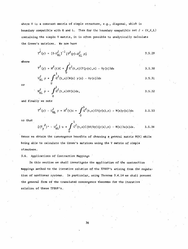
where V is a constant matrix of simple structure, e.g., diagonal, which is
boundary compatible with K and L. Then for the boundary compatible set J = {V,K,L}
containing the simple V matrix, it is often possible to analytically calculate
the Green's matrices. We now have
where
or
Tj(Y) = J
"-UM)-1
frj(Y)-LIKL Y]3.5.29
1
Tj(y) = Hj(t)C + fe(t,$)(F(y(s),$) - Vy(s)}ds 3.5.30
1 0
HJL = jre(t,$){W(s) y(s) - Vy(s)}ds 3.5.31
-K 0
1
UKL fjG(t,$)dV(s)ds,y = 3.5.32
0
and finally we note
1Tj(y) - Uj y Hj(t)c + j(Gj(t,$)(F(y(s),$) - W(s)y(s)1ds 3.5.33
KL0
so that 1
[(T j), - UjL ] u = fe(t,$){(3F/ay)(y(s),$) - W(s)}u(s)ds. 3.5.34
K 0
Hence we obtain the convergence benefits of choosing a general matrix W(t) while
being able to calculate the Green's matrices using the V matrix of simple
structure.
3.6. Applications of Contraction Mappings •
In this section we shall investigate the application of the contraction
mappings method to the iterative solution of the TPBVP's arising from the regula-
tion of nonlinear systems. In particular, using Theorem 3.4.14 we shall present
the general form of the translated convergence theorems for the iterative
solution of these TPBVP's.
36
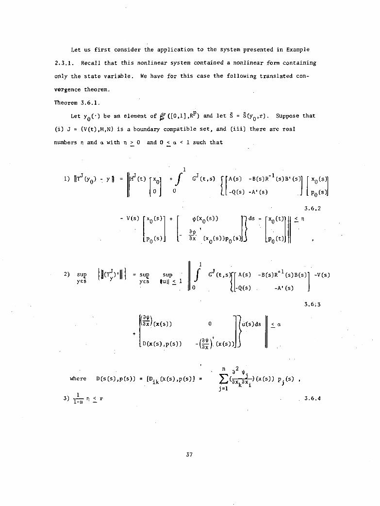
Let us first consider the application to the system presented in Example
2.3.1. Recall that this nonlinear system contained a nonlinear form containing
only the state variable. We have for this case the following translated con-
vergence theorem.
Theorem 3.6.1.
Let yo(•) be an element of ([0,1],RP) and let Š = g(yo,r). Suppose that
(i) J = {V(t),M,N} is a boundary compatible set, and (iii) there are real
numbers n and a with n > 0 and 0 < a< 1 such that
1
1) II (Y0) - Hj(t) + f G (t,$) A(s) -B(s)R-1(s)13'(s)1 xo(s)
0
{xi
0 -Q(s) -A' (s) 130(s)-1
- V(s) xo(s) +[
_
p0 (s)
2) sup 11(TjPill = sup supycs yes pull < 1
0(xo(s))
Ia*_.ax (x
0 (s))p
0 (s).S
ds- -
[Po (t)
3.6.2
<
Gj(t,$)f[A(s) -B(s)R1(s)B(s) -V(s)
0 -Q(s) -A' (s)
where D(s(s),p(s)) = [Dik(x(s),p(s)]
13) 1174 n < r
37
3.6.3
o }u(s)ds <
IPax
(x (s)
na2
tp.
L(ax kax )(x(s)) pi (s) ,
j=1
3.6.4
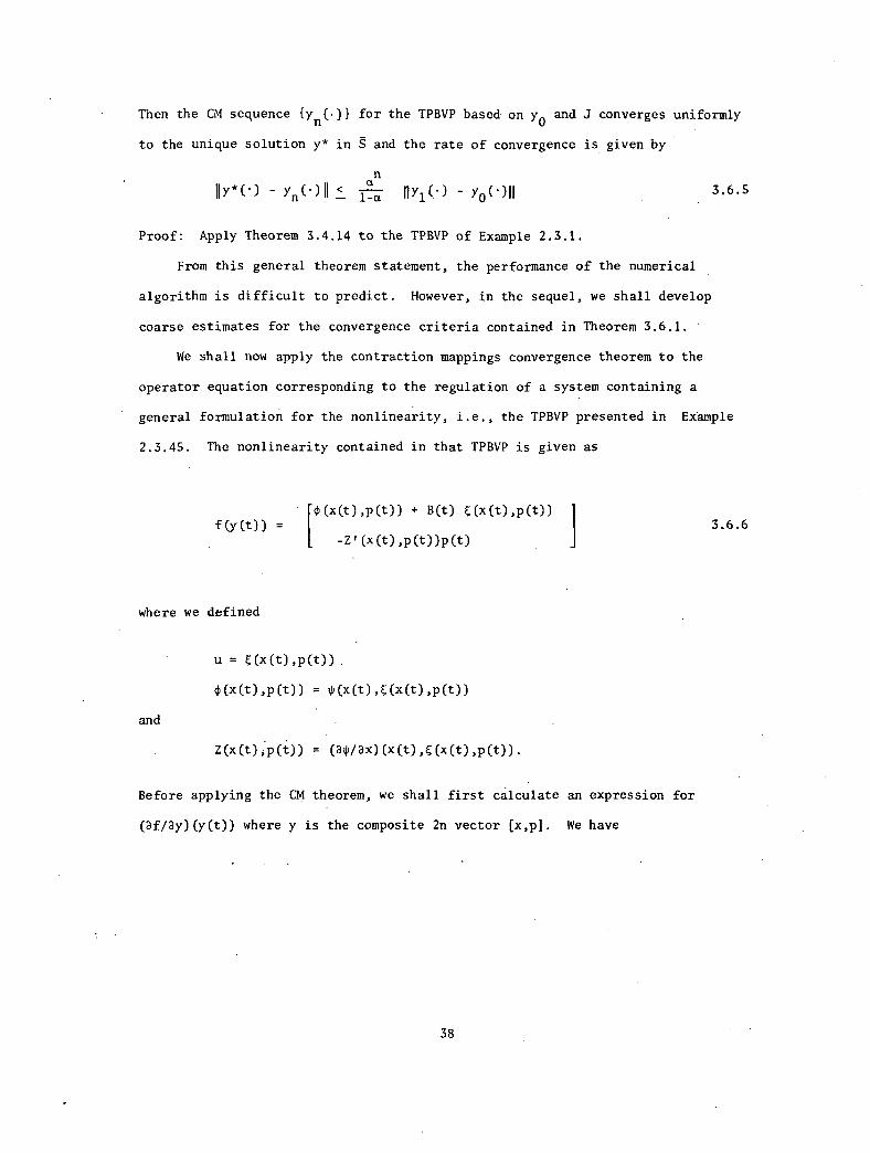
Then the CM sequence {yn(.)} for the TPBVP based on yo and J converges uniformly
to the unique solution y* in g and the rate of convergence is given by
an
HY*(*) - Yn(*)0 1-a 0Y1(*) YO(*)il3.6.5
Proof: Apply Theorem 3.4.14 to the TPBVP of Example 2.3.1.
From this general theorem statement, the performance of the numerical
algorithm is difficult to predict. However, in the sequel, we shall develop
coarse estimates for the convergence criteria contained in Theorem 3.6.1.
We shall now apply the contraction mappings convergence theorem to the
operator equation corresponding to the regulation of a system containing a
general formulation for the nonlinearity, i.e., the TPBVP presented in Example
2.3.45. The nonlinearity contained in that TPBVP is given as
[0(x(t),p(t)) + B(t) (x(t),p(t))f(y(t)) =
(x(t),p(t))p(t)
where we defined
and
n=g0c(t),p(t)).
4(x(t),p(t)) = tp(x(t),g(x(t),p(t))
Z(x(t),p(i)) = (Wax)(x(t)Mx(t),p(t)).
Before applying the CM theorem, we shall first calculate an expression for
(af/3y)(y(t)) where y is the composite 2n vector [x,p]. We have
38
3.6.6
[
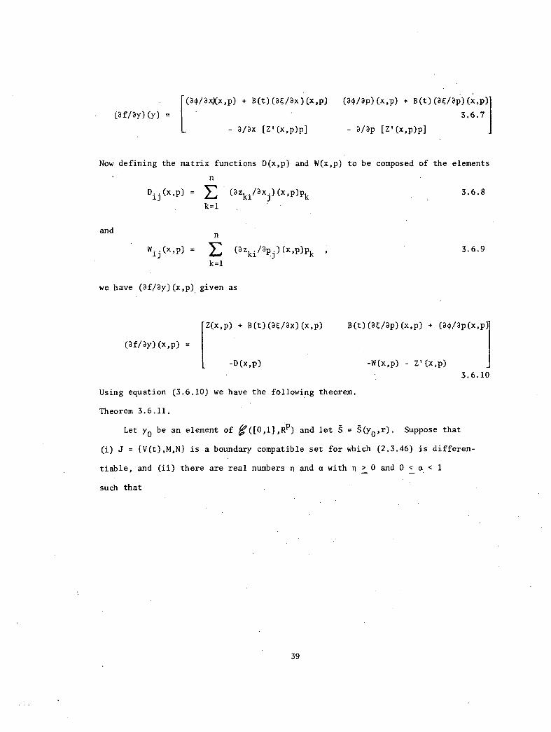
(af/aY)(Y) = 3.6.7
- a/ax [Z'(x,p)p] - a/ap [V(x, )PP]
(a0/ax)(x,p) + 8(t)(n/ax)(x,p) (Wap)(x,p) + B(t)(Wap)(x,p)
Now defining the matrix functions D(x,p) and W(x,p) to be composed of the elements
D..13(x,p) = (az
ki k /ax.)(x,P)P 3.6.8
k=1
and
Wij ..(x,p) = :E: (azkl ./ap))(x ,p)pk ,
k=1
we have (af/ay)(x,p) given as
(af/ay)(x,p) =
3.6.9
[
Z(x,p) + B(t)(aVax)(x,p) B(t)(aC/aP)(x,P) + (a0aP(x,P)
-D(x,p) -W(x,p) - Z'(x,p)
3.6.10
Using equation (3.6.10) we have the following theorem.
Theorem 3.6.11.
Let y0 be an element of gr([0,1],e) and let g = g(yo,r). Suppose that
(i) J = {V(t),M,N} is a boundary compatible set for which (2.3.46) is differen-
tiable, and (ii) there are real numbers n and a with n > 0 and 0 < a < 1
such that
39
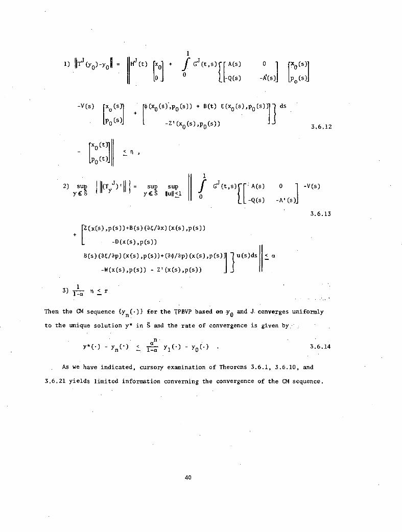
1) =1
Hj (t) [x0 + f j(t,$)t[ A(s) 0 ro(s)]to 0 -Q(s) -g(s) [po(s)]
-V(s) [xo(s1 r (x0(s),p0(s)) + B(t) E(x0(s),p0(s))I] ds
1-130(s)-1 -Z'(x0(s),p0(s))
r130(t10(t)-1
n ,
1
2) sup 10(Tyj)'ll I = sup supy S y E S
3.6.12
I
Gj(t,$)fr. A(s) 0 -V(s)
-Q(s) -A' (s)
[Z(x(s),p(s))+B(s)(aVax)(x(s),p(s))
-D(x(s),p(s))
B(s)(aE/ap)(x(s),p(s))+(aVap)(x(s),p(s)1 } u(s)ds
-W(x(s),p(s)) - Z' (x(s),p(s))
13) 1-a n < r
< a
3.6.13
Then the CM sequence {yn(•)} for the TPBVP based on -y0 and J. converges uniformly
to the unique solution y* in Š and the rate of convergence is given by.
n .
Y*(.) - yn(*) <a1a Y1(*) - Y0{.
3.6.14
As we have indicated, cursory examination of Theorems 3.6.1, 3.6.10, and
3.6.21 yields limited information converning the convergence of the CM sequence.
40

The difficulty to a great extent lies in the intricacy of evaluating the integral
containing the Green's function, Gj(t,$), and the derivative term of tie form
(2F/Dy)(y(s)) - V(s). In the next chapter, we shall consider techniques for
alleviating these difficulties so that meaningful convergence analysis can be
made without extensive computation.

Page intentionally left blank
CHAPTER 4
CALCULATION OF CONVERGENCE CRITERIA
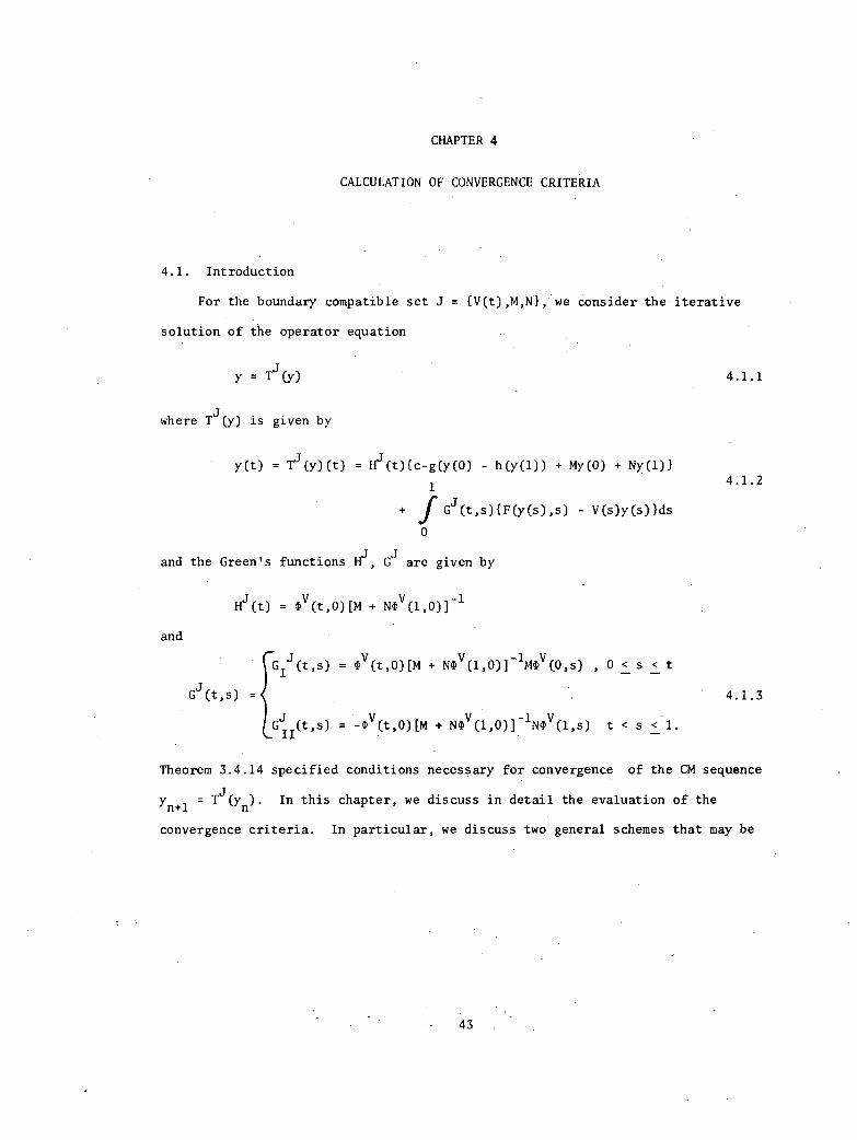
4.1. Introduction
For the boundary compatible set J = {V(t),M,N}, we consider the iterative
solution of the operator equation
Y = Tj(Y)
where Tj(y) is given by
y(t) = Tj(y)(t) = H(t){c-g(y(0) - h(y(1)) + My(0) + Ny(1)}
1
Gj(t,$){F(y(s),$) - V(s)y(s)}ds
0
and the Green's functions Hj, Gj are given by
and
Hj(t) = (t,OHM + N4Y(1,0)]-1
(t,$) = e(t,O)IM + Ne(1,0)] 1MOV(0,$) ,0<s< t
Gj (t,$) = -0V(t,0HM + N(I)v(1,0)] ,$) t < s <
4.1.1
4.1.2
4.1.3
Theorem 3.4.14 specified conditions necessary for convergence of the CM sequence
Yn+1 = Tj(yn).In this chapter, we discuss in detail the evaluation of the
convergence criteria. In particular, we discuss two general schemes that may be
43
used to lessen the analytical difficulties involved in calculating the convergence
parameters n and a.
The first scheme is simply that of selecting.very simple V matrices for use
in the representation. For example, one might select V as the'zero matrix or a
constant diagonal matrix. For these matrices the fundamental matrix is readily
obtained and the Green's function matrices are often easily calculated.
The second scheme involves the use of a similarity transformation. In this
approach, a more general constant V matrix is selected and transformed into a
canonical form. Then using the canonical form, the fundamental matrix is obtained.
However, for this approach, the calculation of the Green's function matrices is
somewhat complicated by the transformation matrices. In conclusion, an approximate
technique is developed which often yields accurate estimates.
4.2. Estimates of Convergence Criteria
Before considering specific boundary compatible sets, we first specify those
estimates of the convergence parameters which are desired. As indicated in
Theorem 3.4.14, the numbers to be calculated are estimates for 1Tj(Y0)-Yo ll
and 11(Tyj)'11 .
First consider the estimation of(y0)-Y0
• At this point, it will be
useful to discuss an effective techniqUe for obtaining the initial estimate of
the solution. Consider the iterative solution of the nonlinear TPBVP •
= F(y,t)
Ky(0) + Ly(1) = c,
4.2.1
and the choice of the boundary compatible set J = ON(t),M,N1 to be used in the
integral representation. Since the boundary conditions of (4.2.1) are linear,
44
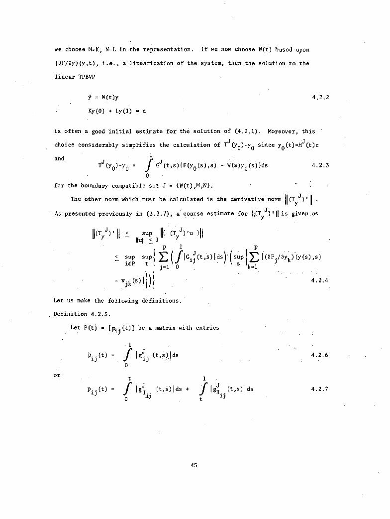
we choose M=K, N=L in the representation. If we now choose W(t) based upon
(3F/3y) (y,t), i.e., a linearization of the system, then the solution to the
linear TPBVP
= W(t)y
Ky(0) + Ly(1) = c
4.2.2
is often a good 'initial estimate for the solution of (4.2.1). Moreover: this
choice considerably simplifies the calculation of Tj(y0)-y0 since yo(t)=Hj(t)c
andTj(y0)-y0 = f
1
Gj(t,$)iF(y0(s),$) - W(s)y0(s)}ds 4.2.3
0
for the boundary compatible set J = {W(t),M,N}.
The other norm which must be calculated is .the derivative norm II (T),J)1 •As presented previ 11(T j)'11ously in (3.3.7), a coarse estimate for is given.as
il(T j) 11 < sup (T J) 'u 111Y Duo < 1 Y
P 1
sup sup{ E (f,G.J(t,$) ds) ( sup I E Jay ) (y(s),$)3.3 k
iEP tj=1 0 s k=1
- v'jks)11)1
Let us make the following definitions.
Definition 4.2.5.
Let P(t) = hoij(t)] be a matrix with entries
or
Pi).(t) g..
0
Pi)..(t) = f0
4.2.4
t,$)Ids 4.2.6
(t ds ign. (t,$)i ds.;
45
4.2.7
where gj and g are elements of GIj(t,$) and G
IIj(t,$) as given in (4.1.3).
ij Hij
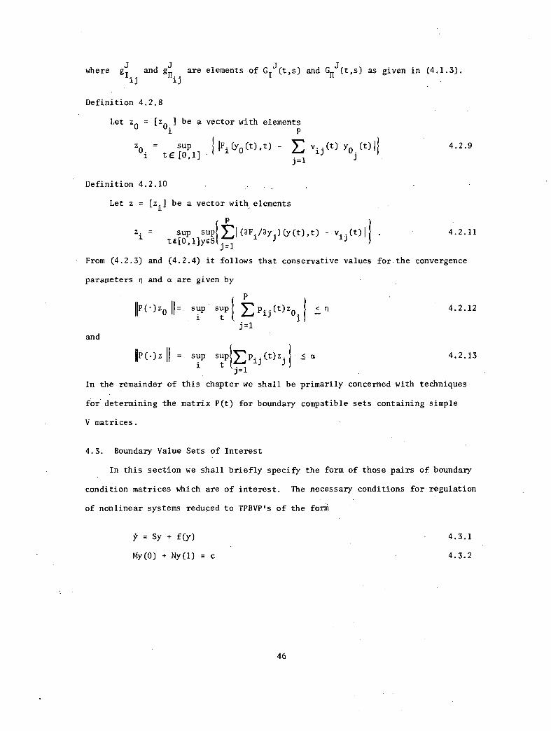
Definition 4.2.8
Let z0 = [zo.] be a vector with elements
zo.
= sup IFi (yo (t) ,t) - v. . (t) yo (t) 11te [0,1] ij
j=1
Definition 4.2.10
Let z = [z.] be a vector with elements
4.2.9
z. sup j suptEl(aF./ay)(y(t),t) - ij(t)11 . 4.2.11
ti[0,1breSj=1
From (4.2.3) and (4.2.4) it follows that conservative values for the convergence
parameters n and a are given by
P
IIP(.)z0 11= sup sup E p ij (t) z
0 I
. < n 4.2.12
33=1
and
OP(.)z sup suptEp..(t)z.} < a 4.2.1313 J
j=1
In the remainder of this chapter we shall be primarily concerned with techniques
for determining the matrix P(t) for boundary compatible sets containing simple
V matrices.
4.3. Boundary Value Sets of Interest
In this section we shall briefly specify the form of those pairs of boundary
condition matrices which are of interest. The necessary conditions for regulation
of nonlinear systems reduced to TPBVP's of the form
ÿ = sy f(Y) 4.3.1
My(0) + Ny(1) = c 4.3.2
46
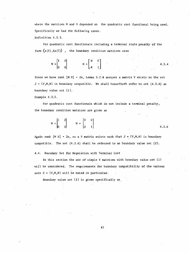
where the matrices M and N depended on the quadratic cost functional being used.
Specifically we had the following cases.
Definition 4.3.3.
For quadratic cost functionals including a terminal state penalty of the
form <x(T),Kx(T)) , the boundary condition matrices were
[ I 0m _1
0 0
0 01N =
[-K I4.3.4
Since we have rank [M N] = 2n, Lemma 3.2.8 assures a matrix V exists so the set
J = {VAN} is boundary compatible. We shall henceforth refer to set (4.3.4) as
boundary value set {1}.
Example 4.3.5.
For quadratic cost functionals which do not include a terminal penalty,
the boundary condition matrices are given as
MI di
[0 0N = L°
ol
11 4.3.6
Again rank [M N] = 2n, so a V matrix exists such that J = {V,M,N} is boundary
compatible. The set (4.3.6) shall be referred to as boundary value set {2}.
4.4. Boundary Set for Regulation with Terminal Cost
In this section the use of simple V matrices with boundary value set {1}
will be considered. The requirements for boundary compatibility of the various
sets J = {VAN} will be noted in particular.
Boundary value set {1} is given specifically as.
47
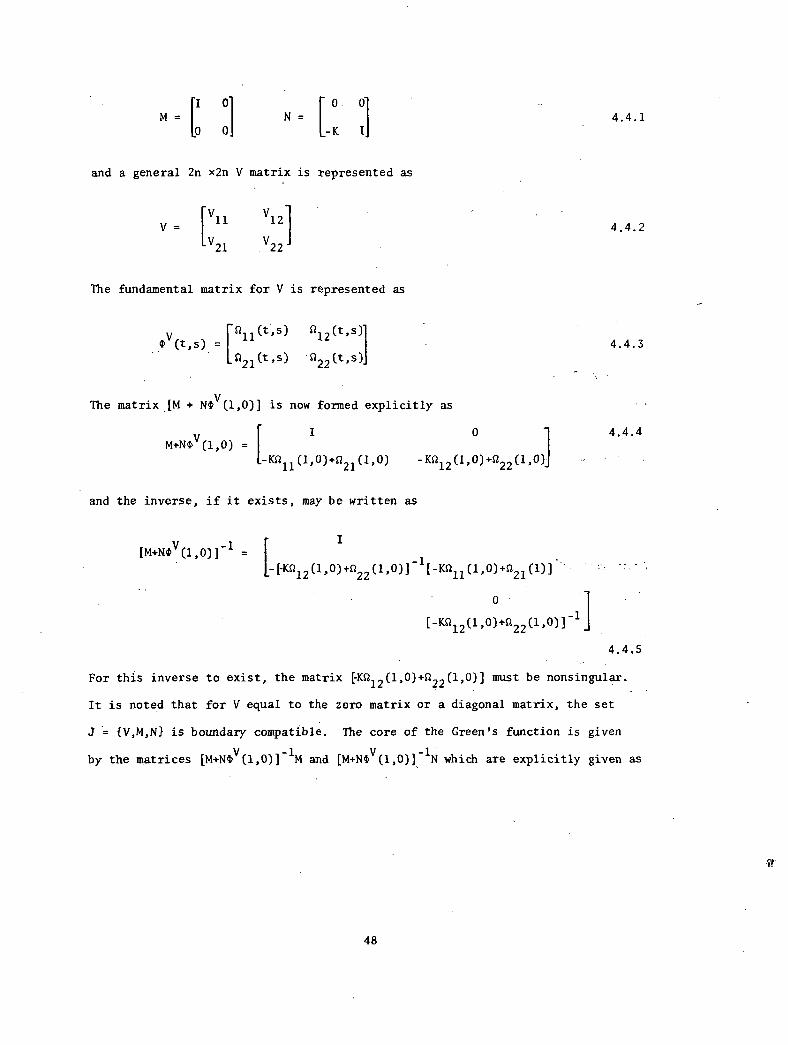
M =I 0
[0 0N[
-K4.4.1
and a general 2n x2n V matrix is represented as
V = [V11
V12
4.4.2V21
V22
The fundamental matrix for V is represented as
[211(t's),$) =
212(t's)14.4.3
SI21(t s) a
22(t s)]
The matrix [M + N4,11(1,0)] is now formed explicitly as
I 0 4.4.4M+N(t
v(1,0) =[
-K011(1'0)+0
21(1,0) -K0
12(1'0)+0
22(1,0)1
and the inverse, if it exists, may be written as
[M+NOV(1,0)]-I =
[-EK012(1'
0)+022(1,0)]-1[-K011(1,0)+021(1)].
0
[-Kg12(1'0)+Q
22(1'0)]-1
4.4.5
For this inverse to exist, the matrix FIGE12(1,0)
+n22(1,0)] must be nonsingular.
It is noted that for V equal to the zero matrix or a diagonal matrix, the set
J = {VAN} is boundary compatible. The core of the Green's function is given
by the matrices [M+101/(1,0)] IM and [M+Ntv(1,0)]
-1 N which are explicitly given as
48
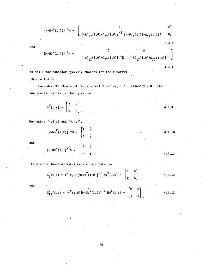
[M+N0V(1,0)]-1MI
'-f-°12(1,o)+222(1,o)]-1
[-KC/ 11(1'
0)44221)1'0)]
and
[Mi-N0V(1,0)]-1N
We shall now consider specific
Example 4.4.8.
4.4.6
-4-012 (1' 0)+O
22 (1' 0)]-1K I[-Kn
12)1'0)+0
22(1'0)]-1
4.4.7
choices for the V matrix.
Consider the choice of the simplest V matrix, i.e., assume V = O. The
fundamental matrix is then given as
I 00V (t,$) =
[ I0, 4.4.9
I .
Now using (4.4.6) and (4.4.7),
[1,44.Ncly(1,0)]-1m =
and
ol[IK
o4.4.10
0 0[M+N0V(1,0]-
{
-K I . 4.4.11
The Green's function matrices are calculated as
0]G(t' s) = (t,0)[M+N0 (1,0)]
-1 MOV(0,$) =
I
and
{I
K 04.4.12
GII(t's (t,0)[M+N0
V (1,0)]
-1Ne(1,$) -
[04.4.13
49
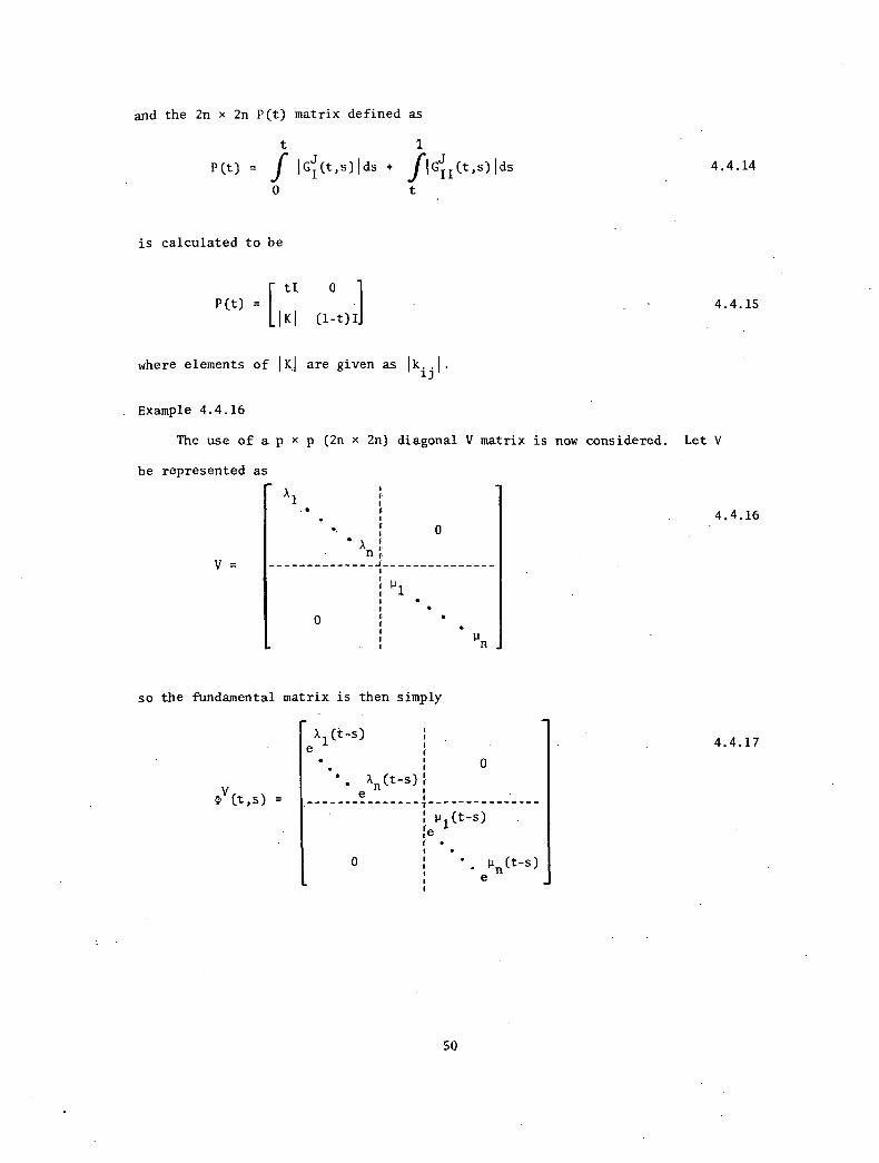
and the 2n x 2n P(t) matrix defined as
1
P(t) = f lei(t,$)Ids + II (t' s)lds
0
is calculated to be
[ tI 0P(t)
IK1 (1-01
where elements of 1K] are given as lkij. .1.
4.4.14
4.4.15
Example 4.4.16
The use of a p x p (2n x 2n) diagonal V matrix is now considered. Let V
be represented as
V =
1
•
.n
04.4.16
o
so the fundamental matrix is then simply
1(t-s)
4.4.17
0
• Xn(t-s)e
p1(t-s)
ie•
• ' Pn(t-s)e
50
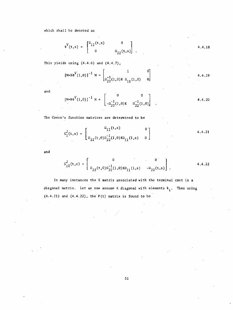
which shall be denoted as
o(1)V(t,$) =
r11(t's)
0 R22(t,$)]
•
This yields using (4.4.6) and (4.4.7),
[M+N0V (1,0)]
-1 M =
R22(1'0)K
11(1,0)
and0
[M+N(DV(1,0))-1 N =[
--022-1(1,0)K
221(1'
The Green's function matrices are determined to be
and
o
0)
Ril(t,$) 0 1
Gi(t,$) =R
-1(1 ,0)KR (1,$) 0 ]22(t,0)0
2211
0
GII(t's) = -122(t' 0)Q
22 (1' 0)KR
11 (1' s) -
022(t,$)
In many instances the K matrix associated with the terminal cost is a
diagonal matrix. Let us now assume K diagonal with elements ki. Then using
(4.4.21) and (4.4.22), the P(t) matrix is found to be
51
4.4.18
4.4.19
4.4.20
4.4.21
4.4.22
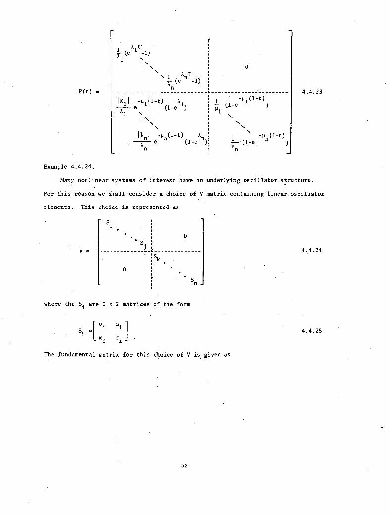
P(t) =
ax1t
(e -1). 1
t1-1-(e
n -1)
'n
1K1
-p1(1-t)
1
X1 e (1-e )
\
Ikn I -1.1n(1-t)
e (1-e n)n
0
(1-t))111
1 -Pn(1-t)P
(1-e )n
4.4.23
Example 4.4.24.
Many nonlinear systems of interest have an underlying oscillator structure.
For this reason we shall consider a choice of V matrix containing linear.oscillator
elements. This
V -
choice is represented as
S ,1 .
i. 1 0* S I(
J (r.
k
4.4.24
0
n
where the S. arei
2
a.
x 2 matrices
co.
of the form
S. = 1 4.4.25-w. Q.
The fundaMental matrix for this choice of V is. given as
52
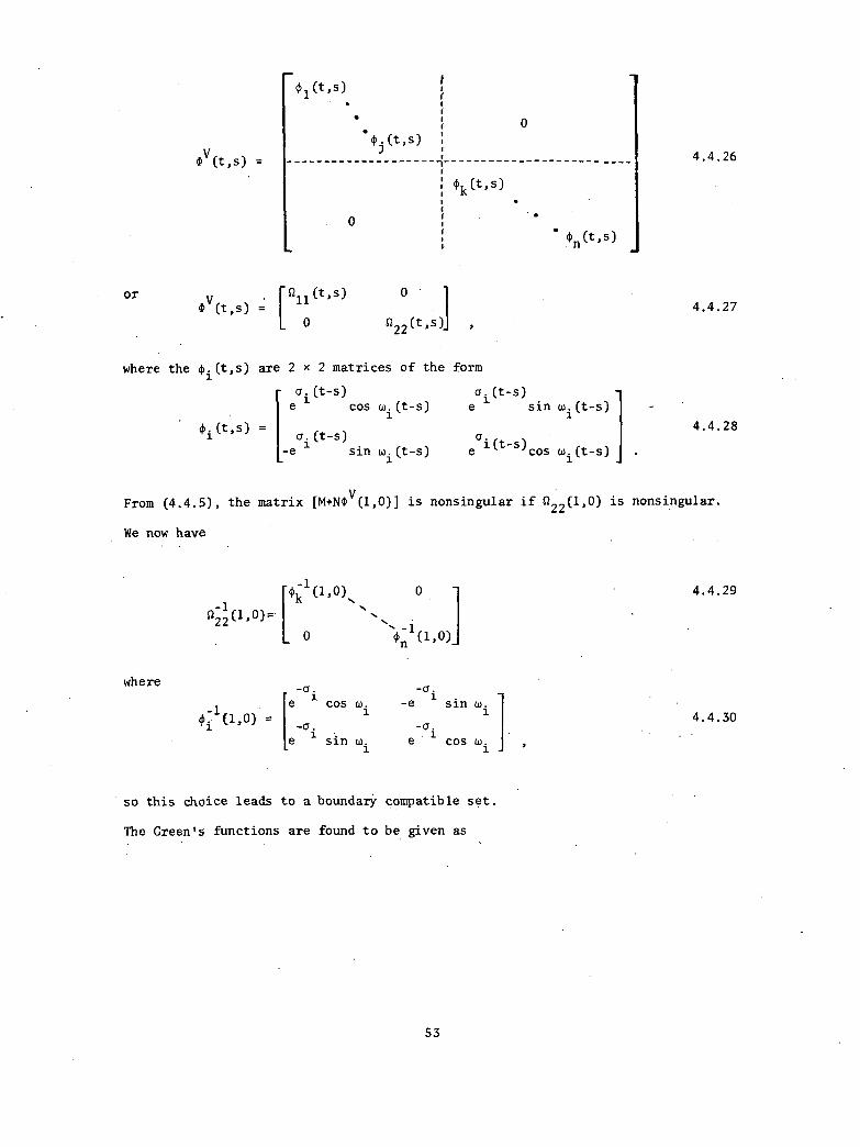
or
, ) =
v(t,$) =
(I)1(t s)
•
o
o
(Pk (t's)
(Pn(t,$)
/NS
011(t s)
o
where the 11)i(t,$) are 2 x 2 matrices of the form
a.(t-s) a.(t-s)1
1 ie cos w.(t-s) e sin w.(t-s)1
- sin wi(t-s)
(t,$) - (t-s) a.1(t-s)
COS w.(t-s)
4.4.26
4.4.27
4.4.28
From (4.4.5), the matrix [M+NOV(1,0)] is nonsingular if 022(1,0) is nonsingular.
We now have
where
0 cpn (1,0)]22(1'(3)= _
-a. -a.cos w. -e sin w.
-1 e 1
1 1
1Oi (1,0) =
- -a.
e ai 1sin w. e cos w.
1 1
so this choice leads to a boundary compatible set.
The Green's functions are found to be given as
53
4.4.29
4.4.30
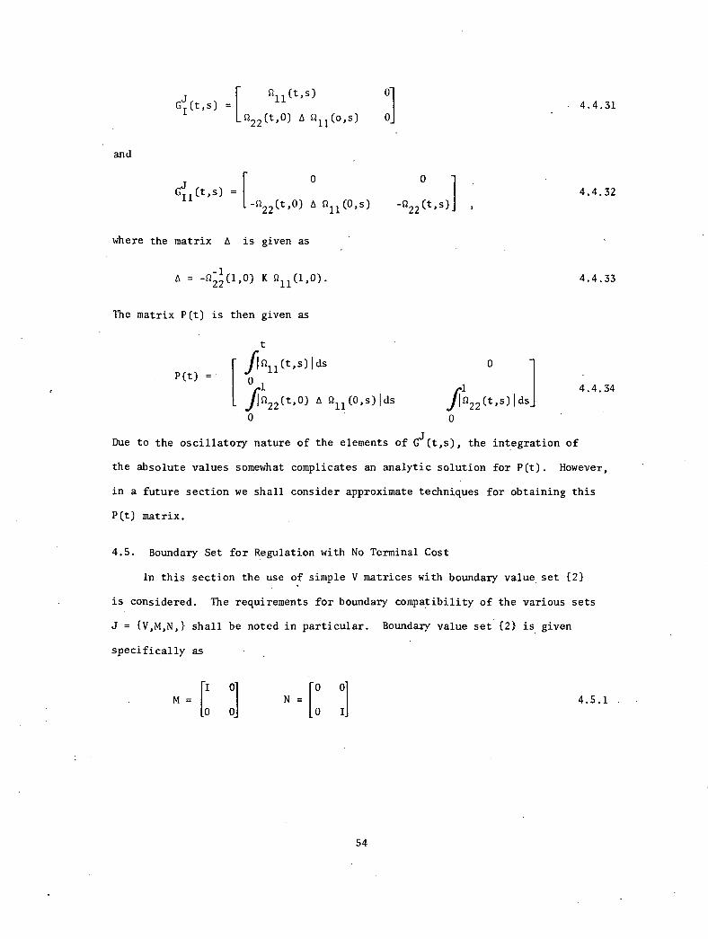
and
GI(t's) =
Q22(t'0) A Q
11(o s)
GII(t's)
0
-022(t'0) A R
11(0's)
where the matrix A is given as
A = .4222(1'0) K
11(1'0).
The matrix P(t) is then given as
P(t) =
[11(t s)
t
[fIS1n(t,$) Ids 0
0
-Q22(t's)]
01 4
JIR22(t,0) A Q (0,$)Ids
JI5222(t's) Ids
0 0
Due to the oscillatory nature of the elements of G (t,$), the integration of
the absolute values somewhat complicates an analytic solution for P(t). However,
in a future section we shall consider approximate techniques for obtaining this
P(t) matrix.
4.4.31
4.4.32
4.4.33
4.4.34
4.5. Boundary Set for Regulation with No Terminal Cost
In this section the use of simple V matrices with boundary value set {2}
is considered. The requirements for boundary compatibility of the various sets
J = {V,M,N,} shall be noted in particular. Boundary value set {2} is given
specifically as
I 0
M 10 0N = 4.5.1
0 I
54
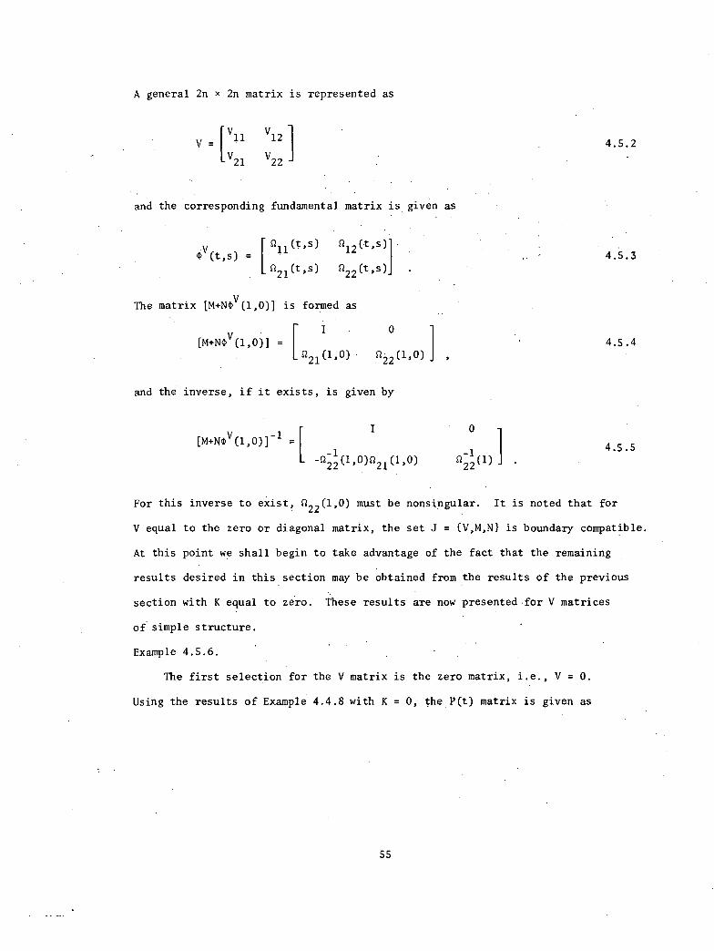
A general 2n x 2n matrix is represented as
V = V11 1112
V1121 22
and the corresponding fundamental matrix is given as
4.5.2
Q11(t's) Q 12(t's)(Dv(t,$) = 4.5.3
021(t's) 222(t's) •
The matrix [M+MV(1,0)] is formed as
[M+NOV(1,0)] =
[ 221(1'0) . S1
22 (1' 0)
and the inverse, if it exists, is given by
[[M+NOV(1,0)]-1 =-1 1
-Q22(1,0)0
21(1,0) Q
22(1)
4.5.4
4.5.5
For this inverse to exist, 022(1,0) must be nonsingular. It is noted that for
V equal to the zero or diagonal matrix, the set J = {V,M,N} is boundary compatible.
At this point we shall begin to take advantage of the fact that the remaining
results desired in this section may be obtained from the results of the previous
section with K equal to zero. These results are now presented for V matrices
of simple structure.
Example 4.5.6.
The first selection for the V matrix is the zero matrix, i.e., V = 0.
Using the results of Example 4.4.8 with K = 0, the P(t) matrix is given as
55
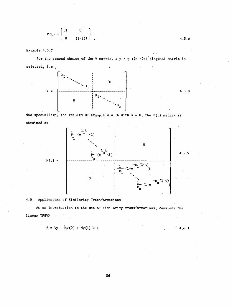
[tI 0P(t)
0 (1-t)I . 4.5.6
Example 4.5.7
For the second choice of the V matrix, a p x p (2n x2n) diagonal matrix is
selected, i.e.;
V -n
0
n
4.5.8
•Now specializing the results of Example.4.4.16 with K 0, the P(t) matrix is
obtained as
P(t) =
AL (e 1
t -1)
X1
0
0
-P1(1-t)(1-e
n
(l_e -pn(1-t))
4.5.9
4.6. Application of Similarity Transformations
As an introduction to the use of similarity transformations, consider the
linear TPBVP
= Vy My(0) + Ny(1) = c . 4.6.1
56
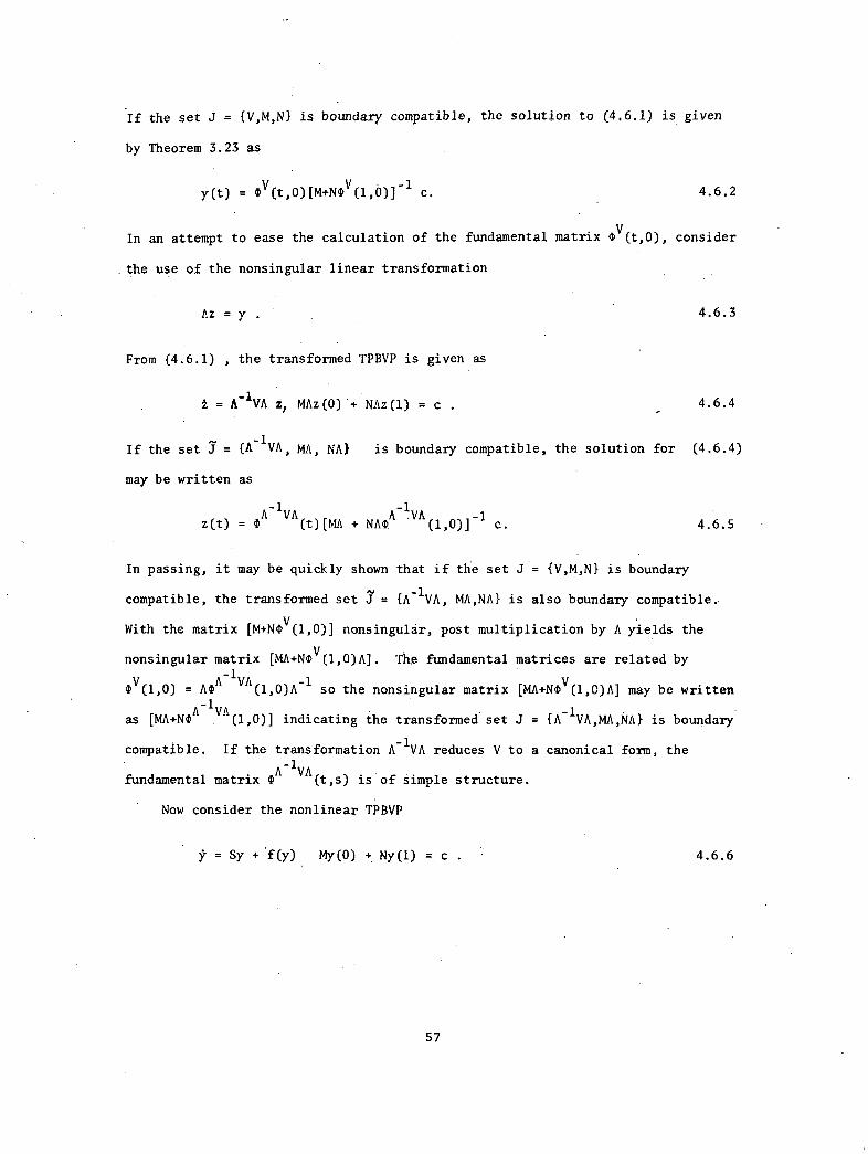
If the set J = {V,M,N} is boundary compatible, the solution to (4.6.1) is given
by Theorem 3.23 as
y(t) = OV(t,0)[M+NOV(1,0)]-1 c. 4.6.2
In an attempt to ease the calculation of the fundamental matrix 0V(t,0), consider
the use of the nonsingular linear transformation
Az = y . 4.6.3
From (4.6.1) , the transformed TPBVP is given as
= A-1
VA z MAz(0) + NAz(1) = c . 4.6.4
If the set I = {A-1VA, MA, NA} is boundary compatible, the solution for (4.6.4)
may be written as
-1 -1z(t) = 0
A VA (t)[MA + NAtA
VA(1,0)]
-1 c. 4.6.5
In passing, it may be quickly shown that if the set J = {VAN} is boundary
compatible, the transformed set I= {A-1VA, MA,NA} is also boundary compatible.
With the matrix [M+N0V(1,0)] nonsingular, post multiplication by A yields the
nonsingular matrix [MA+N0V(1,0)A]. Tho fundamental matrices are related by
A-1
VAv(1,0) = A0 (1,0)A-1 so the nonsingular matrix [MA+NOV(1,0)A] may be written
A-1
VAas [MA+N0 (1,0)] indicating the transformed set J = {A
-1VA,MA,NA} is boundary
compatible. If the transformation A-1
VA reduces V to a canonical form, the
A-1
VAfundamental matrix (t,$) is of simple structure.
Now consider the nonlinear TPBVP
= Sy + f(y) My(0) + Ny(1) = c . 4.6.6
57
Again consider the nonsingular linear transformation
and let
A z = y
-LD = A VA .
Then (4.6.6) becomes the transformed TPBVP
= A-1 SAz + A 1f(Az)
MAz(0) + NAz(1) = c .
4.6.7
4.6.8
4.6.9
If the set j = {A-1VA, MA, NA} is boundary compatible, the integral representation
for (4.6.9) is
1
TI(y) = H(t)c + j G5(t,$)(A 1SAz + A-1 f(Az(s)) - Dz}ds
0
where the Green's functions are given as
and
I7(t) =D(t,0)[MA+NAO
D(1,0)]
-1
D(t,0)[MA + NAO
D(1,0)]
-1MI)D(0,$) , 0<s< t
G (t,$) =1- -4) (t,0)[MA + NA4)
D(1,0)]
-1N4) 1,$) , t < s < 1 .
4.6.10
4.6.11
4.6.12
If it is desired to investigate the iterative solution of the operator equation
z = T (z) ,
the operator derivative CFz is given as
4.6.13
1(TzI )'u = j(G
J (t,$)(A
-1SAz(s) + A
-1(3f/3y)(Az(s))A - D}u(s)ds 4.6.14
0
58
if the TPBVP is differentiable. However, rather than using (4.6.14), another
approach may be taken It may easily be shown that a direct relationship exists
between the Green's functions for the boundary compatible set J = {V,M,N} and
the transformed boundary compatible set J = {D,MA,NA} . In particular,
and
Hj(t,$) = AH5(t,$) 4.6.15
Gj(t,$) = AG(t,$)A-1
I
GII(t,$)= AGIIet,$)e
1
4.6.16
4.6.17
Hence the integral representation for (4.6.6) may be written as
1
y(t) = Tj(y)(t) = AITT(t,$)c + jrAe(t,$)A-1{Sy(s)+f(y(s),$)-Vy(s)lds
0 4.6.18
Then if the matrix A-1
VA is a canonical form, (I)D(t,$) and G (t,$) are often much
easier to calculate, and it may very well be easier to calculate estimates for
(T J)'
The theory of canonical forms has received great attention in the past years.
General books of interest include Gantmacher [G1], Bodweig [B2],Turnbull [T1],
and Ferrar [F2]. Of interest to control analysts are the books of Bellman [B1]
and Ogata [01]. In particular, we now present a well known theorem concerning
the diagonalization of matrices.
Theorem 4.6.19
IfthecharacteristicrootsX.of the matrix V are distinct, there exists
a matrix A such that
59
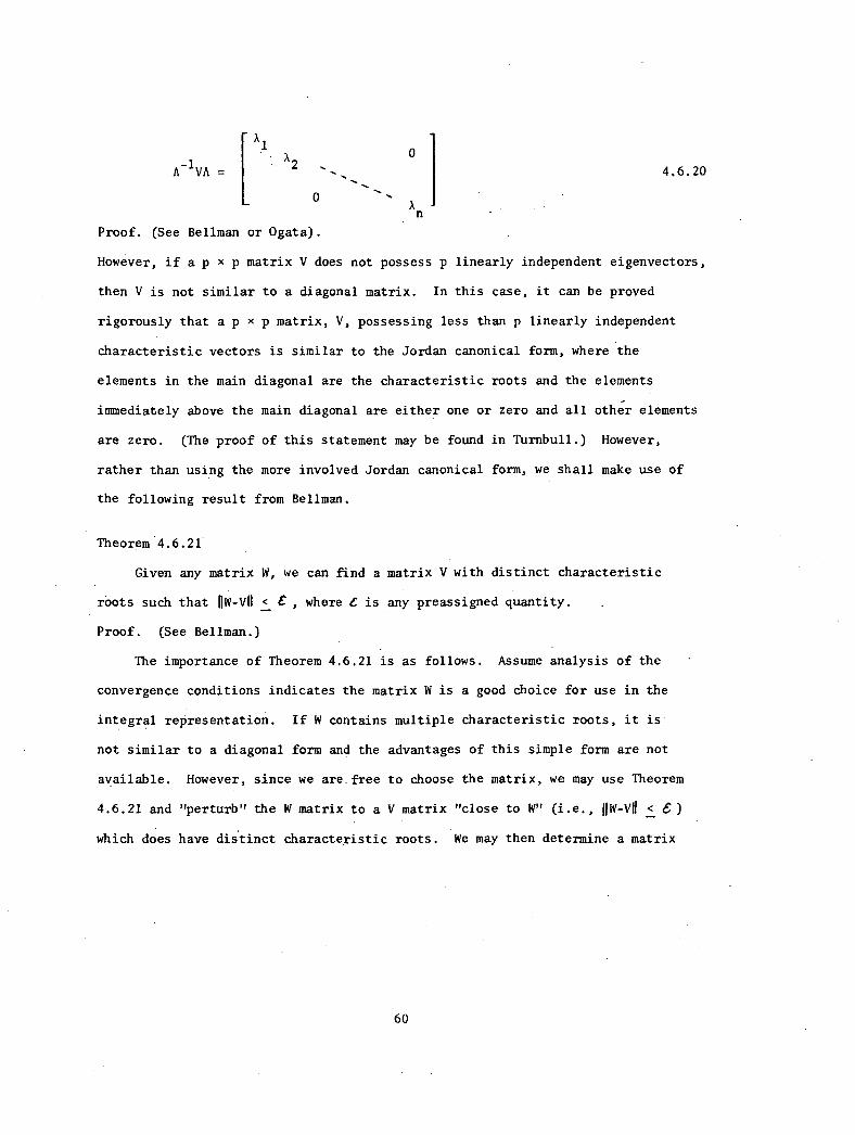
A-1
VA = 4.6.20
Proof. (See Bellman or Ogata).
However, if a p x p matrix V does not possess p linearly independent eigenvectors,
then V is not similar to a diagonal matrix. In this case, it can be proved
rigorously that a p x p matrix, V, possessing less than p linearly independent
characteristic vectors is similar to the Jordan canonical form, where the
elements in the main diagonal are the characteristic roots and the elements
immediately above the main diagonal are either one or zero and all other elements
are zero. (The proof of this statement may be found in Turnbull.) However,
rather than using the more involved Jordan canonical form, we shall make use of
the following result from Bellman.
Theorem 4.6.21*
Given any matrix W, we can find a matrix V with distinct characteristic
roots such that BW-VO < e , where C is any preassigned quantity.
Proof. (See Bellman.)
The importance of Theorem 4.6.21 is as follows. Assume analysis of the
convergence conditions indicates the matrix W is a good choice for use in the
integral representation. If W contains multiple characteristic roots, it is
not similar to a diagonal form and the advantages of this simple form are not
available. However, since we are.free to choose the matrix, we may use Theorem
4.6.21 and "perturb" the W matrix to a V matrix "close to W" (i•e. < e )
which does have dis'tinct characteristic roots. We may then determine a matrix
60

Not only does D have only real elements but, more significantly, K-1
A-1
and
AK have only real elements. Now setting
A = AK
A-1
= K-1
A-1
4.6.27
the transformation is given the standard form of
D = A VA . 4.6.28
As a result of this discussion, in the sequel the term canonical form shall
specifically refer either to diagonal or to the modified diagonal form as in
(4.6.24).
We shall now choose several forms for the V matrix to illustrate the use
of the similarity transformation with the boundary value sets of interest.
Example 4.6.29.
Let us consider
M =I 0
0 0
the boundary value
N =
set
0 0
-K I4.6.30
and the 2n x 2n V matrix with distinct characteristic roots
V =[0
V11
4.6.31V22
The similarity transformation has the form
A =[A
11 0 1
0 A22
-1 [AilA .
0
A-1
0 22
4.6.32
62
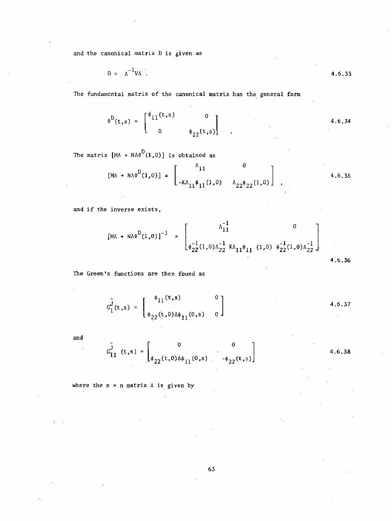
and the canonical matrix D is given as
D = A 1 V
The fundamental matrix of the canonical matrix has the general form
(1)D(t,s r
il(t,$)
0
o
4)22(t,$) •
The matrix [MA + NAOD(1,0)] is obtained as
[MA + NA0(1,0)] =
and if the inverse exists,
+ NA(I,D(1,0)]
-1
A11
0
[-KA11011(1'0) A cp (1 0)1 ,
22 22 '
0
022(1'0)A
22 KA11011
(1,0) (I)22(1,0)A22
The Green's functions are then found as
4,11(t,$) 0
Gi(t,$) =
(1) (t'°)411 (0,$) 0
GjI (t' s) =
I
0
(t,0) "11(O's)
where the n x n matrix 6 is given by
63
-02:(t,$)]
4.6.33
4.6.34
4.6.35
4.6.36
4.6.37
4.6.38
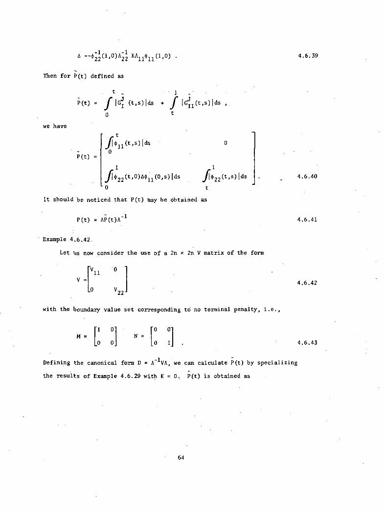
-1 -1° —4'22(1,O)A22 KA114)11(1,0) .
Then for P(t) defined as
we have
- •
P(t) = f l G I j ' sflds + f 1GII '
(t sflds
0
P(t) =
t
t.1 ds°11(t-s)l01 0
1 1
/*
:22(t,O)"11(o's)1.1 1.ds
.11:22 (t,$)Ids
0 t
It should be noticed that P(t) may be obtained as
P(t) = AP(t)A-1
Example 4,6.42
Let us now consider the use of a 2n x 2n V matrix of the form
V =
[1/11
0 V22
with the boundary value set corresponding to no terminal penalty, i.e.,
rI 0M = LO 0] N = 0 I]
Defining the canonical form D = A-1
V , we can calculate P(t) by specializing
the results of Example 4.6.29 with K = 0, P(t) is obtained as
64
4.6.39
4.6.40
4.6.41
4.6.42
4.6.43
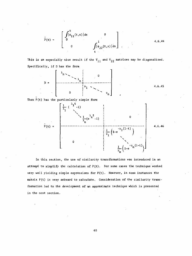
J11011(t,$)Ids 0
P(t)1
0 jr022(t,$)Ids
4.6.44
This is an especially nice result if the V11
and V22
matrices may be diagonalized.
Specifically, if D has the form
nD =
Then P(t) has the particularly simple form
P(t) =
1 t( 1 -1)
1 ••\
1 Xnt
7.--(e -1)^n
un
0
0
1 -u1(1-t) )
1-e
••
•
4.6.45
4.6.46
1 (1 e
7pn(1-t)\
Pn
In this. section, the use of similarity transformations was introduced in an
attempt to simplify the calculation of P(t). For some cases the technique worked
very well yielding simple expressions for P(t). However, in some instances the
matrix P(t) is very awkward to calculate. Consideration of the similarity trans-
formation led to the development of an approximate technique which is presented
in the next section.
65
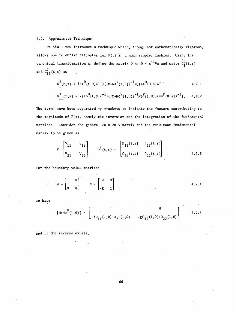
4.7. Approximate Technique
We shall now introduce a technique which, though not mathematically rigorous,
allows one to obtain estimates for P(t) in a much simpler fashion. Using the
canonical transformation A, define the matrix D as D = A-1
VA and write GiJ(t,$)
and GII(t,$) as
GI(t,$) = {A(1)
D(t,O)A
-1}{[M+N(1)
V (1,0)]
-I M}{A0
D (0,$)A
-1 } 4.7.1
GjI (t' s) = -{A.1)
D(t,O)A
-1}{[M+NO (1,0)] 1N4Y(1,0)}{A(I)
D(0,s)A
-1 }. 4.7.2
I
The terms have been separated by brackets to indicate the factors contributing to
the magnitude of P(t), namely the inversion and the integration of the fundamental
matrices. Consider the general 2n x 2n V matrix and the resultant fundamental
matrix to be given as
V =V11 V12
V21
V22
t,$) =
[ 5111(t,$) 5212(t,$)
5221(t's) 222(t's) • 4.7.3
For the boundary value matrices
0 0 01M =
[IN[
4.7.4
we have
0 0 -K I]
I 0[M+NO
v(1,0)] = 4.7.5
-K011(1,0)+0
21(1,0) _Kn
12 (1,0)+0
22(1,0)
and if the inverse exists,
66
[M+NOV(1,0)]-1I
-[-m12(1,°)+° 11-1
22(''' (1.°)+'
0
[-KO (1,0)12 +222(1'0)1
The center bracketed terms are then found as
and
[
I 0[M+NOV(1,0)]-1 M =
A 0
[M+NlY(1,0)]-1 NrDV(1,0) =
where the n x n matrix A is given as
0 0]
-A I
A = -pm12(1,0)+°22(1,0)14[-m11(1,0)+Q21(1,0)1.
(1,0)]
4.7.6
4.7.7
4.7.8
4.7.9
Now assuming that (I)D(t,$) represents the primary magnitude characteristics of
AOD(t,$)A
-1 , we shall form
and
{4)D(t,0)1{[M+N(1)
V (1,0)]
-1 M}{(1)
D(0,$)}
-(4)D(t,0)}{[M+N(1)
V (1,0)]
-1 N4Y(1,0)}{(1)
D(0,$)}
4.7.10
4.7.11
as approximations to GI(t,$) and G11(t,$). Following the discussion in Section 4.6
concerning canonical forms, the fundamental matrix 0D(t,$) may be represented in
the form
67
(I)D(t,$) =
[PIL(t,$) 0
o 022(t s)] 4.7.12
Using (4.7.10) and (4.7.11), we obtain the approximations
4111(t's)Gj(t,$)z. 4.7.13
and
D2 (t,0),64
D 1(0,$) 0
2
0 0Gj (t,$)
[
4.7.14O2 (t,O)A0D
1 (0,$)
(1'22(t's)2
Finally, this yields
D 1 ' (t s)lds 0
1
P (t)1
4.7.15
fle22(t,0)6ppli (0,$) ids 0D22 (t , s ) ds
For the boundary value set
01 0M =
[IN =
[04.7.16
0 0.1 0 I ,
we may specialize the results of (4.7.15) with K = 0 to obtain
68
where
P (t)1( SD 'sflds
0I 11
le (t' 1 0)4D
1 ' (0 s)lds flAD
2'.' r's'
ldsl'222
A = 4122(1'0)0
21(1'0) .
4.7.17
4.17.18
These approximations greatly simplify the calculation of P(t), and moreover, they
capture the primary quantitative behavior of the P(t) matrix. The concepts and
techniques introduced in this chapter will be illustrated in several numerical
examples in Chapter 6.

Page intentionally left blank
CHAPTER 5
CONTROLLABILITY FOR NONLINEAR SYSTEMS
5.1. Introduction
The concept of null controllability is a natural aspect of the study of
optimal regulation for nonlinear systems. Whereas the optimal regulator attempts
to drive the system from its initial state into a region near the origin, null
controllability is concerned with driving the system precisely to the origin.
Historically, the issues of regulation and controllability are closely intertwined.
The study of linear regulator problems in a general framework served to uncover
some of the underlying relationships that exist between the structure of the
optimal system and the fundamental concept of controllability [K1], [K3]. Much
of the effort to date concerning null controllability of nonlinear systems has
involved determination of feedback controllers such that the driven systems
satisfy certain Lyapunov-type stability arguments [B4], [G3]. In this chapter
the integral representation of TPBVP's and the contraction mapping theorem will
be used to investigate the controllability of nonlinear systems via existence of
solutions arguments.
5.2. Controllability for Linear Systems.
As an introduction to the controllability issue and the approach to be
taken in the study, we shall first consider the controllability of linear systems.
71.
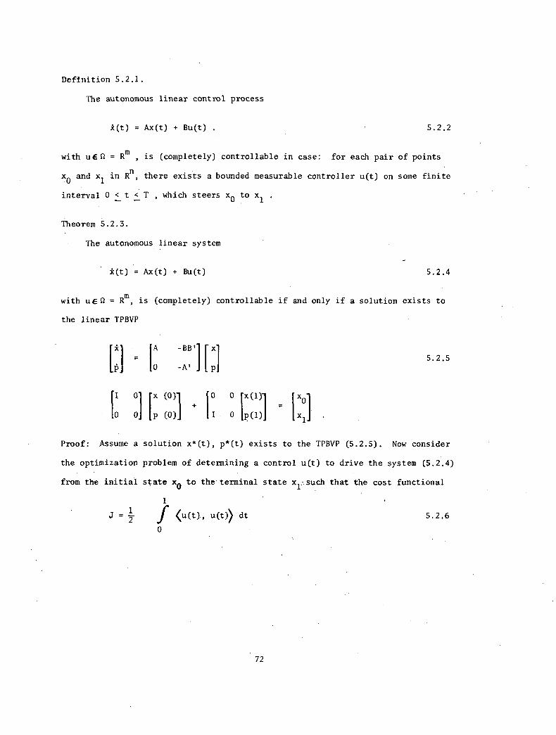
Definition 5.2.1.
The autonomous linear control process
k(t) = Ax(t) + Bu(t) . 5.2.2
with ue St = Rm , is (completely) controllable in case: for each pair of points
x0
and x1 in R
n, there exists a bounded measurable controller u(t) on some finite
interval 0 < t < T which steers x0 to x1 .
— —
Theorem 5.2.3.
The autonomous linear system
k(t) = Ax(t) + Bu(t) 5.2.4
with uE D= Rm, is (completely) controllable if and only if a solution exists to
the linear TPBVP
[kJ
IA -BB] [1
0 -A' p
1 0 (01 0 0 tx(, x00 01 p (0) I 0 lp(1) x1•1
•
5. 2.5
Proof: Assume a solution x*(t), p*(t) exists to the TPBVP (5.2.5). Now consider
the optimization problem of determining a control u(t) to drive the system (5.2.4)
from the initial state xo to the terminal state x1 such that the cost functional
11
J = 2 — f <u(t), u(t)) dt
0
72
5.2.6
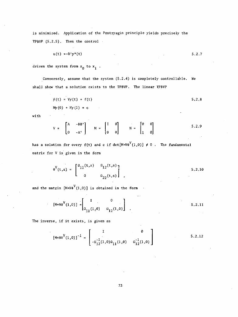
is minimized. Application of the Pontryagin principle yields precisely the
TPBVP (5.2.5). Then the control
u(t) =-B'p*(t) 5.2.7
drives the system from x0 to xl .
Conversely, assume that the system (5.2.4) is completely controllable. We
shall show that a solution exists to the TPBVP. The linear TPBVP
with
y(t) = Vy(t) + f(t)
My(0) + Ny(1) = c
[A -B131V =
1
0 -A'M =
0 0N =
o
has a solution for every f(t) and c if det[M+Ne(1,0)] # 0 . The fundamental
matrix for V is given in the form
tlY(t,$) = 1211(tis)L o
and the matrix [M+Ne(1,0)] is obtained in the form
I 0[M+Ne(1,0)] =
211(1'0) 2
12(1'0)]
The inverse, if it exists, is given as
I o[M+NclY(1,0)]-1 = -1
-212(1'o)n11
-1(1 o) '12(1.°)
73
5.2.8
5.2.9
5.2.10
5.2.11
5.2.12
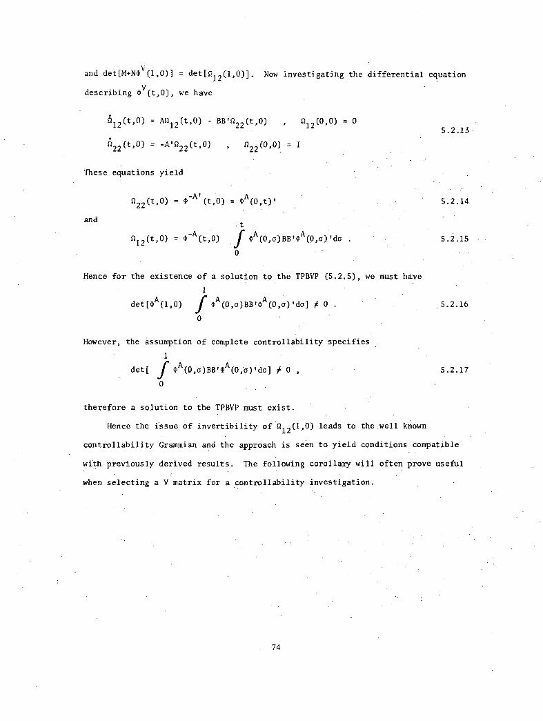
and det[M+N0V(1,0)] = det[1212(1,0)]; . Now investigating the differential equation
describing 0V (t,0), we have
Q12(t PS2(t0)22 ,612(t'°)
= A0) - B 012(0'0) 0
622(t,0) = -A,52
22(t,0) , 0
22(0'0) = I
These equations yield
and
-A'2(t,0) = (t,0) = 0
A(0,t)'
012(t,0) =
-A(t,0) f
A(0,a)B
B'0,
A(0,0)'da .
0
Hence for the existence of a solution to the TPBVP (5.2.5), we must have
1
det[0A(1,0) f
A(0,a)BB,0
A(0,o)'da] # 0 .
0
However, the assumption of complete controllability specifies
1
det[A(0,a)BB'0
A(0,0)'da] # 0 ,
0
5.2.13
5.2.14.
5.2.15
5.2.16
5.2.17
therefore a solution to the TPBVP must exist.
Hence the issue of invertibility of 5212(1,0) leads to the well known
controllability Grammian and the approach is seen to yield conditions compatible
with previously derived results. The following corollary will often prove useful
when selecting a V matrix for a controllability investigation.
74
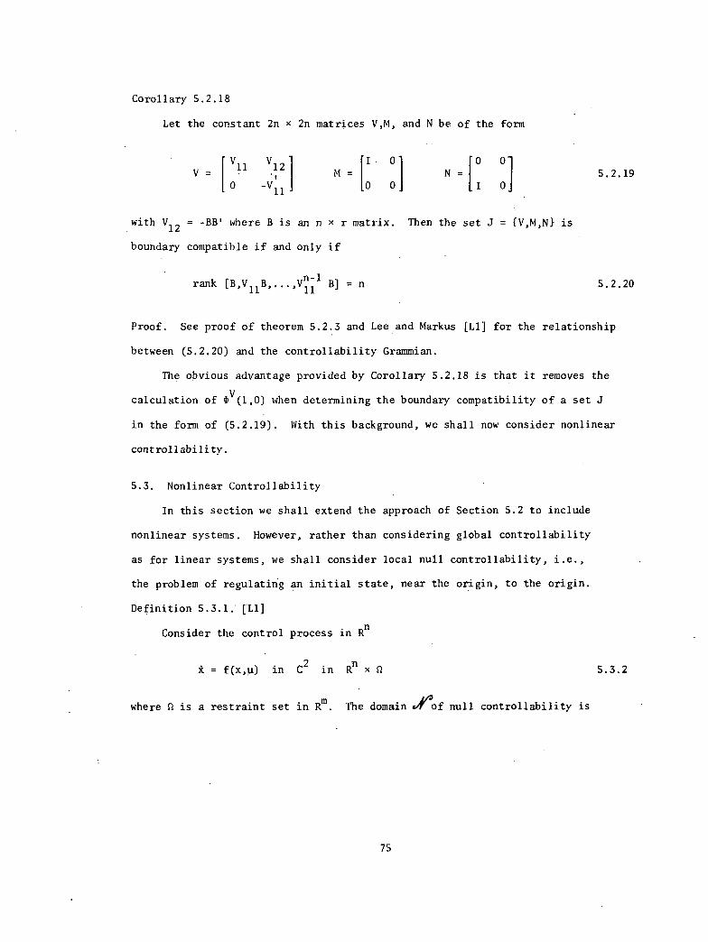
Corollary 5.2.18
Let the constant 2n x 2n matrices V,M, and N be of the form
V11
V 0 1 0 0V = • M = Il N0 -V11 0 0] II 0
with V12
= -BB' where B is an n x r matrix. Then the set J = {VAN} is
boundary compatible if and only if
rank [B,V11
B,...,V11 B] = n
1
5.2.19
5.2.20
Proof. See proof of theorem 5.2.3 and Lee and Markus [L1] for the relationship
between (5.2.20) and the controllability Grammian.
The obvious advantage provided by Corollary 5.2.18 is that it removes the
calculation of e(1,0) when determining the boundary compatibility of a set J
in the form of (5.2.19). With this background, we shall now consider nonlinear
controllability.
5.3. Nonlinear Controllability
In this section we shall extend the approach of Section 5.2 to include
nonlinear systems However, rather than considering global controllability
as for linear systems, we shall consider local null controllability, i.e.,
the problem of regulating an initial state, near the origin, to the origin.
Definition 5.3.1. [L1]
Consider the control process in Rn
= f(x,u) in C2
in Rn x 5.3.2
where S3 is a restraint set in Rm. The domain Yrof null controllability is
75
defined as the set of all points x0 E R
n, each of which can be steered to x
1 = 0
by some bounded measurable controller u(t) c:n in finite time. If AContains
an open neighborhood of xl = 0, then (5.3.2) is said to be locally controllable
(near the origin). We shall now consider the null controllability of nonlinear
systems by means of integral representations.
Theorem 5.3.3.
Consider the control process in Rn
= f(x,u) in C2
in Rn x
with u = 0 interior to the restraint set 0 C:11111 .
Assume
(a) f(0,0) = 0
(b) rank [B,AB,...,An-1
B] = n
where A = (3f/3x)(0,0) and B = (3fPu)(0,0)
Then the domainceof null controllability is open in Rn.
Proof. Let us define the function gx,u) as
so that
and
5.3.4
5.3.5
5.3.6
5.3.7
gx,u) = f(x,u) - Ax - Bu 5.3.8
4)(0,0) = 0
.311,(---) (0' 0) = 0
Dx
311,(---)(0' 0) = 0 .
Du
5.3.9
5.3.10
5.3.11
Now consider the optimization problem composed of the system
76
ic = Ax + Bu + 11)(x,u) , 5.3.12
the boundary conditions,
x(0) = x0 , x(1) = 0 , 5.3.13
and the cost functional
11
J = 2 — f (u(t),u(t)) dt. 5.3.14
0
The Hamiltonian for this problem is given by
1H =
2 — (u(t),u(t)) + (Ax(t),p(t)) (Bu(t),p(t))
and the costate variable is described by the differential equation
(x.,u) ,p (t))
5.3.15
p = A'p - (x,u)p . 5.3.16
Now assume a control of the form
u = -B'p 5.3.17
accomplishes the desired transfer. The canonical system of equations is now
given as
ic = Ax - BB'p + gx,u(p)) 5.3.18
= -Alp - (a)( (x,u(p))p 5.3.19
subject to the boundary conditions
77
1 I 01 lx(0)1 0 [x(1)1 x 10 0 0 p(0) II 0 [p(1)] I 0.1
This may be expressed as
where
and
= Sy + F (y)
MY(0) + Ny(1) = c
A -BB' 1S =
0 -A'
F(y) = [
M =
- (x,u(P))PI ••alp
114x,u(P))
N = C =
5.3.20
5.3.21
5.3.22
5.3.23
For the boundary compatible set J = {V,M,N} where M and N are given in (5.3.22),
the solution to (5.3.20) may be written as
1
y(t) = Hj(t)c + fe(t,$)(Sy(s) + F(y(s)) - V(s)y(s)}ds
0
or as an operator equation
Y = Tj(Y).
5.3.24
5.3.25
Clearly with c = 0, y(-) = 0 is a fixed point of T . We are now interested in
the existence of a solution, y(.), if c is varied in a neighborhood of the origin.
Define the variable z as
z = P (c,y) . 5.3.27
78
It is seen that a zero of Pj is a fixed point of T. We shall now show that
(P )' (0,0) has a bounded inverse and the desired conclusions concerning the
existence of a solution y may be deduced from the implicit function theorem.
(For presentations of the implicit function theorem, see Kantorovich [K4] and
Holtzman [H1]). The operator derivative is given as
or
1BF
(Pj)' (0,0)v(t) = v(t) - Gj(t,$){5 + (--)(0) - V(s)}v(s)ds 5.3.28
0
(Pj)' (0,0)v = [I-Dj]v .
BFIf the set 3" = IS + (--)(0), M,N,} is boundary compatible, then [I-Dj]
-1 is
Dy
bounded and is given as (see Falb [F1])
where
5.3.29
[I-Dj]-1 v = v 5.3.30
1
R3
= BF
Jr. j(t,$){V(s) - S - e--)(0)1 v(s)ds.By0
5.3.31
DFA11 that now remains is to show that 3% {s (--)(0),M,N1 is boundary compatible.
By
We have
and
[
li(x,u(p))
F(Y) = a,- (i--;c) ' (x,u(p))17.
4(u)(x,u(P))
alp-
3 7,-,[(-57)'(x,u(p))pl
79
4(--)(x,u(P))Bp
D 4--4(--P(x.u(P))13]ap Bx
5.3.32
5.3.33
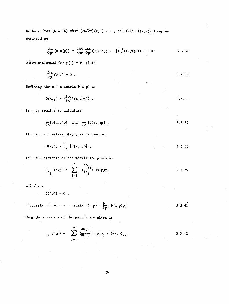
We have from (5.3.10) that (3Vax)(0,0) = 0 , and (atp/ap)(x,u(p)) may be
obtained as
alp alp au af(—ap)(x,11(1))) = (—au)(7-p)(x,u(P)) = -[(7-u)(x,u(P)) - BDP
which evaluated for y(.) = 0 yields
(---)(0,0) = 0 .ap
Defining the n x n matrix D(x,p) as
D(x,p) = 4P(x,u(p)) ,
it only remains to calculate
;R[D(x,p)p] and ap [D(x,p)p] .
If the n x n matrix Q(x,p) is defined as
aQ(x,p) = .57 [D(x,p)p] ,
Then the elements of the matrix are given as
and then,
n
cik(x,p) = L.
Q(0,0) = 0 .
apk,
(x,P)p-i
Similarly if the n x n matrix r(x,p) = a
[D(x,p)p]
then the elements of the matrix are given as
naDki
y .(x p) = (ap. )(x,p)pj p(x,p)ki •
j=1 1.
80
5.3.34
5.3.35
5.3.36
5.3.37
5.3.38
5.3.39
5.3.41
5.3.42
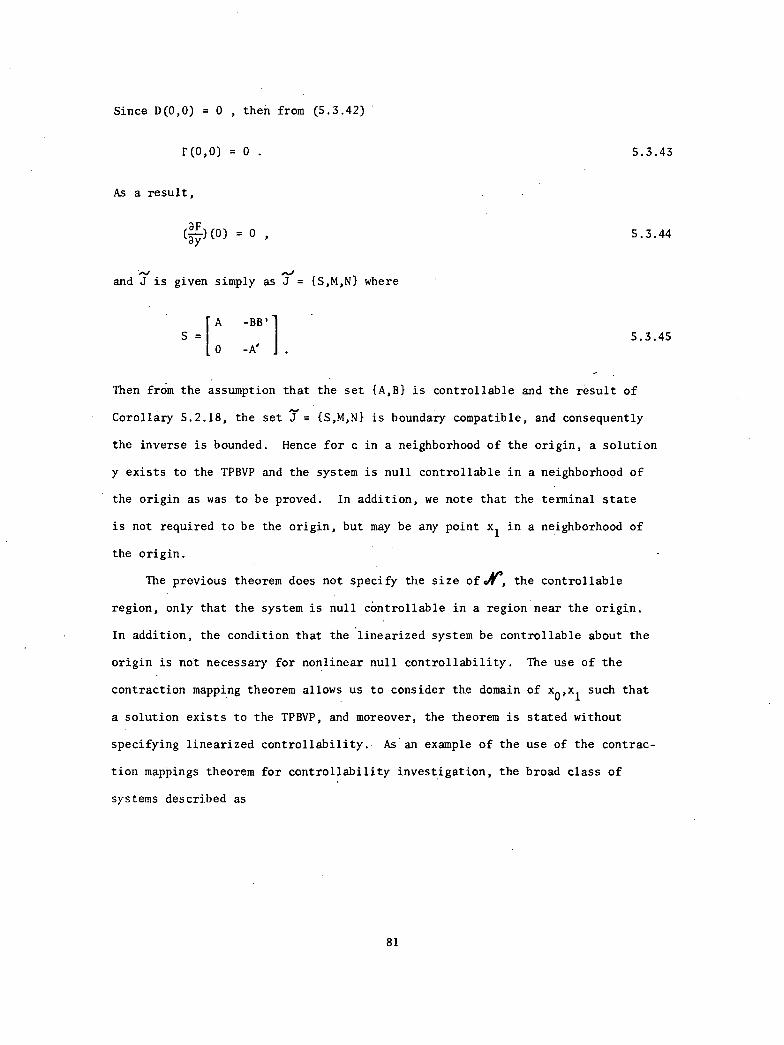
Since D(0,0) = 0 , then from (5.3.42)
r(o,o) = o .
As a result,
3F(—) (0) = 0 ,3y
and J is given simply as J = {SAN} where
A -BB'S =
0 -A' .
5.3.43
5.3.44
5.3.45
Then from the assumption that the set {A,B} is controllable and the result of
Corollary 5.2.18, the set .7= {SAN} is boundary compatible, and consequentlythe inverse is bounded. Hence for c in a neighborhood of the origin, a solution
y exists to the TPBVP and the system is null controllable in a neighborhood of
the origin as was to be proved. In addition, we note that the terminal state
is not required to be the origin, but may be any point xl in a neighborhood of
the origin.
The previous theorem does not specify the size ofir, the controllable
region, only that the system is null controllable in a region near the origin.
In addition, the condition that the linearized system be controllable about the
origin is not necessary for nonlinear null controllability. The use of the
contraction mapping theorem allows us to consider the domain of x0'
x1 such that
a solution exists to the TPBVP, and moreover, the theorem is stated without
specifying linearized controllability. As an example of the use of the contrac-
tion mappings theorem for controllability investigation, the broad class of
systems described as
81
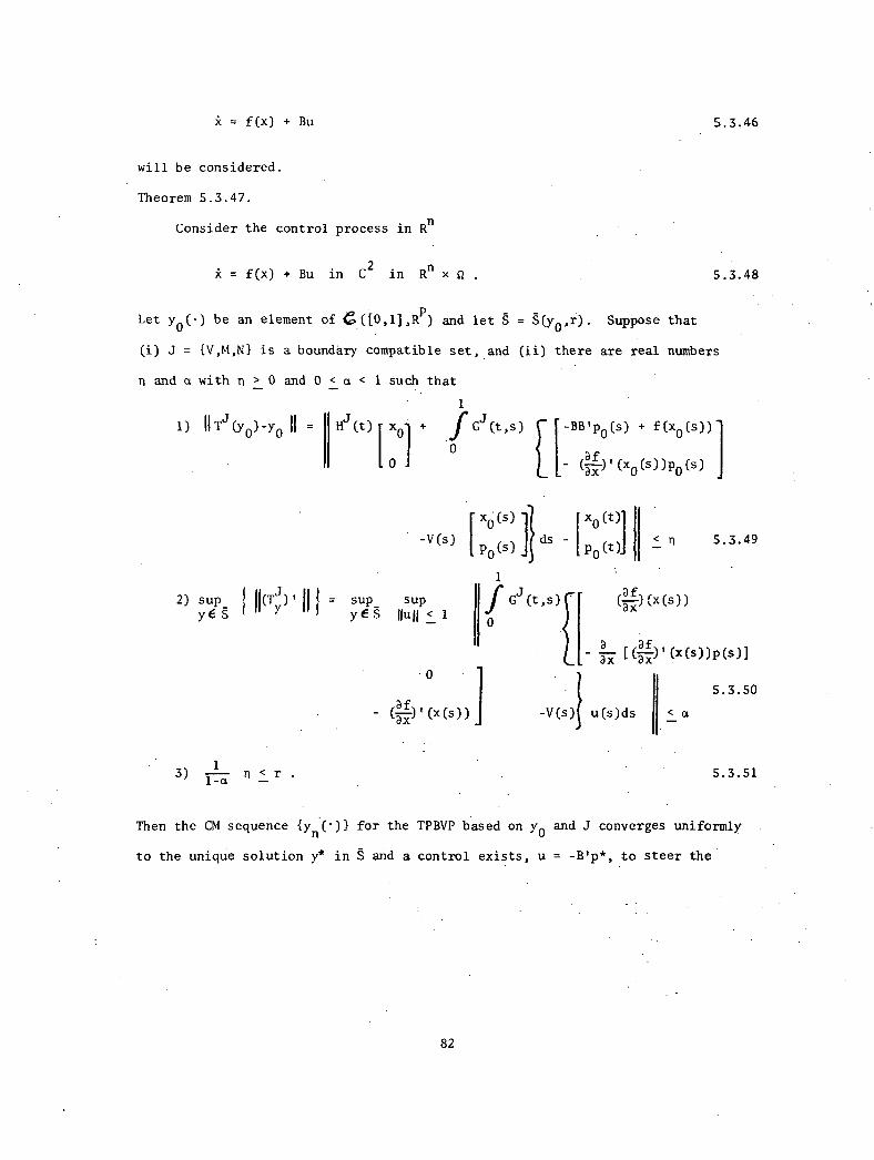
= f(x) + Bu 5.3.46
will be considered.
Theorem 5.3.47.
Consider the control process in Rn
x f(x) + Bu in C2 in Rn x
Let yo(-) be an element of 4;([0,1],e) and let g = g(yo, . Suppose that
5.3748
(i) J = (V,M,N1 is a boundary compatible set, and (ii) there are real numbers
n and a with n > 0 and 0
1) IlTj(y0)-y0 II =
< a < 1 such that
1
(t) xol
0
+ Gj (t,$)
I 0
-V(s)
2) sup_ / 11(T;)' sup_ supyE g • y E S Hun < 1
0
af- (rip (x(s))
3) 11
<a — n r .
[-BB'po(s) + f(x0(s))1
af- (ye (xo(s))po(s)
xo(s)1 1 )(0(01ds -
PP) PO "
1
f Gj(t,$)il
0
3x
< n
(uf)(x(s))
5.3.49
[(4)1 (x(s))p(s)]
-V(s) u(s)ds <
5.3.50
5.3.51
Then the CM sequence {yil(*)} for the TPBVP based on y0 and J converges uniformly
to the uniqUe solution y* in 8 and a control exists, u = -B'p*, to steer the
82
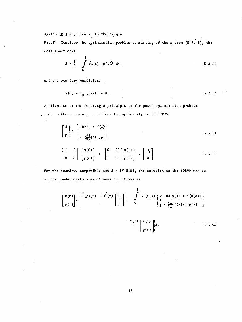
system (5.3.48) from x0
to the origin.
Proof. Consider the optimization problem consisting of the system (5.3.48), the
cost functional
=21
1
f<u(t), u(t)> dt,
0
5.3.52
and the boundary conditions
x(0) = x0 , x(1) = 0 . 5.3.53
Application of the Pontryagin principle to the posed optimization problem
reduces the necessary conditions for optimality to the TPBVP
1 -BB'p + f(x)I
a- e-
fd ' (x)p
I 01 lx(0)1 [0 0.1 [ x(1) }
0 0 p(0) I 0 p(1)
5.3.54
5.3.55
For the boundary compatible set J = {VAN}, the solution to the TPBVP may be
written under certain smoothness conditions as
lx(t) 0
] Tj(y)(t) = Hj(t) [x
p(t) 0
1
f Gj(t,$) -BB'p(s) + f(x(s))
af-t-c) (x(s))p(s)
- V (s) x(s)ds
p(s)
83
5.3.56
Applying contraction mappings Theorem 3.4.14 to the operator (5.3.56) yields
the conditions to be proved in Theorem 5.3.47.
For the general system formulation, k = f(x,u), the canonical equations
of 2.3.54 are used subject to the boundary conditions (5.3.55). Techniques for
calculating the criteria of Theorem 5.3.47 will now be considered.
5.4. Evaluation of Controllability Convergence Parameters
In Section 4.6, the variables z0'
z, and P(t) were defined such that coarse
estimates for n and a were obtained as
andn =
• a = .017(.)z .
5.4.1
5.4.2
In this section we shall consider the determination of z0, z, and P(t) for
the controllability Theorem 5.3.47. In particular, the conditions for boundary
compatibility and the use of simple V matrices and similarity transformations
will be considered.
The boundary value set for controllability problems is given as
oN =I oi
Assuming a general form for the .2n x 2n V matrix and the fundamental matrix
OV(t,$), i.e.,
[ V =
V11
V12
v v21 22
211(t's) C12(t's)v(t,$) =
The matrix [M+NOV(1,0)] is obtained as
84
1 221(t's) C122(t's) '
5.4.3
5.4.4
be used in the integral representation.
[M+NOV(1,0)] is given as
[M+10V(1,0)]-1 =
I
If det[212(1,0)]
1
0 ,
-1 2) 2-212(1 '11' (12) D (112 '
0)1
and then the core matrices of the Green's function are given as
and
o[wisloV(1,0]-11,4
-1-4.212
(1,0) 5211(1,0) 0
[[M+N(01(1,0)]-1N4Y(1,0) =
0 0
Q12 (1' 0)
11 (1' 0) I
[M+NdY(1,0)] =SI11(1'0) 52
12(1'0) .
5.4.5
This yields det[M+NOV(1,0)] = det[5212(1,0)]. Hence the condition for boundary
compatibility reduces to the nonsingularity of D12(1,0). In passing, it is seen
that neither the zero matrix nor a diagonal matrix (nor a modified diagonal) may
the inverse of
5.4.6
5.4.7
5.4.8
Since the boundary value set (5.4.3) disallows the use of particularly simple
V matrices, we shall consider an approximate technique for calculating Gj(t,$)
and P(t) for V matrices of general structure.
Example 5.4.9.
Using the canonical transformation
D = A-1
VA ,
85
5.4.10
the Green's function matrices are given as
G/(t,$) = {A(1)D(t,0)A-1
}{[M+N(1)V(1,0)]-1M}{A~D(O,$)A-1}
GII(t's) = {Ad?D(t,O)A
-1 }i[M+N(01(1,0)] 110V(1,0)}(A(1)
D(0,$)A
-11
5.4.11
5.4.12
for the boundary compatible set J = {VAN}. From (5.4.7) and (5.4.8), the
center bracketed terms in (5.4.11), (5.4.12) are given as
I 0[M+N(01(1,0)]-1M = 5.4.13
and
A 0
0 0[M+N(DV(1,0)] 1N4Y(1,0) = 5.4.14
where
-A I
A = -5212
1(1' 0) 52
11 (1' 0) 5.4.15
Assuming that (I)D(t,$) represents the primary magnitude characteristics of
AOD(t,$)A
-1 , approximations for G
I(t,$) and GII(t,$) are formed as
G, (t,$)D(t,0)[M+10
v(1,0)]
-1 /0
D (0,$)
and
5.4.16
Gj (t,$)D(t,0)[M+N(1) (1,0)]-1N(IY(1,0)(1)
D(0,$) . 5.4.17
Following the discussion in Section 4.6, V is chosen such that e(t,$) is
diagonal or modified diagonal and may be represented as
D 4)11(t,$)(t,$) = 5.4.18.
0 4)22(t's)1 •
86
Using this form of 0(t,$) in (5.4.16) and (5.4.17), the approximations for
yt,$) and G11(t,$) are given as
and
D011(t,$) 0
0D 2 1 (t,0) tap
D 1(0,$) 0
0 0
GII(t's) DAO
11(0,$)
4)22(t'O) °22(t's)1
The approximation for P(t) is then given as
where
P(t);;,-
- tfl D011(t,$)Ids0
(t,0) Aell
(0,$)Ids
A = -5212(1'0) 52
11(1,0) .
0
1
f l(pD22(t ,$) Ids
t
5.4.19
5.4.20
5.4.21
5.4.22
For D a diagonal matrix, P(t) given by (5.4.21) becomes a particularly simple
form. Several variables are now defined which will be used with P(t) to calculate
estimates for n and a in Theorem 5.3.47.
Definition 5.4.22.
Using the boundary compatible initial estimate, y0(t) = Hj(t)c, define the
2n vector z0
as
87
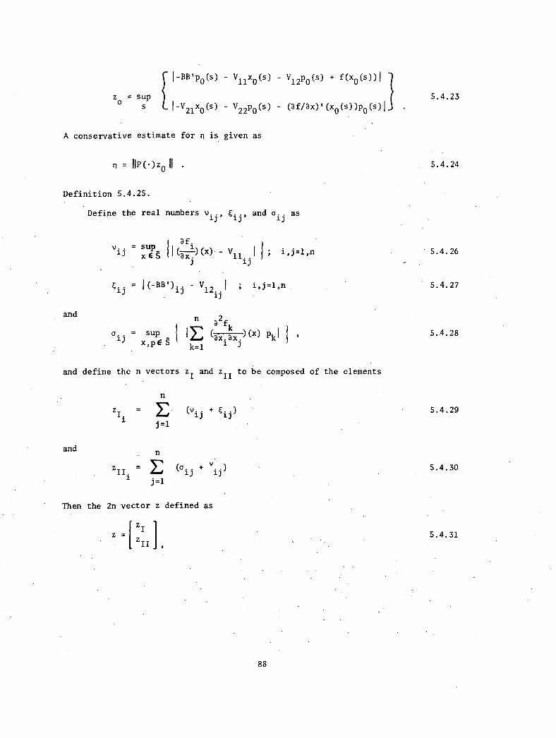
[
1-BB'p0(s) - V11x0(s) -
V12p0(s) + f(x0(s))1
z --. sup 5.4.23
I -V21x0(s) v22p0(s) - ofl2xF(x0(s))po(s)1
A conservative estimate for n is given as
n = HP(.)zo . 5.4.24
Definition 5.4.2S.
Define th erealnumbersv,Eand
vi4 = supixe51`3x.'`
asij ij, Gij
ir 3f„• iVll..l
5.4.26l i
x) - j=1- • 'n
"3
Ei=1(-1313')
ij
and
..aij
= sup
- V12.
1 ; i,j=1,nj
ij
n 2f
I ILE]
-5.4.27
5.4.28(axl .)(x) Pk' '
x,pe S k=1
and define the n vectors zI and z
II to be composed of the elements
n
(v . ij . + E .
1). ) 5.4.29
j=1
and n
zII.
= I: ij
5.4.30
j=1
Then the 2n vector
z =1 z
IzII
z defined as
,5.4.31
88

may be used with P(t) to obtain a coarse estimate for a as
a = .
Numerical evaluation of the convergence criteria is presented for various
examples in Chapter 6.
-89
:
5.4.32

. Page Intentionally Left Blank
CHAPTER 6
ITY ICAL EXAMPLES
6.1. Introduction
We examine the regulation and control of several nonlinear systems to
demonstrate the usefulness of contraction mappings and to illustrate the practical
applications of the major theorems. There are many well known and very powerful
iterative methods for the solution of optimal control problems. However, practical
convergence criteria are few and far between. In this chapter we demonstrate
that general results may be obtained via the application of the contraction
mappings convergence theorem. In addition, the practical application of the
contraction Mapping algorithm demonstrates that in many cases it is an efficient,
straightforward technique for the solution of optimal control problems. The
examples demonstrate that practical application has a much broader range than
the theoretical results might imply. This is primarily due to the coarse
estimates which are used to evaluate the convergence parameters.
The first example to be considered is the regulation of the well known
Van der Pol equation. As an illustrative exercise, both contraction mappings
and modified contraction mappings are applied to this problem. The results
obtained are compared with previously published data. The second example
begins a two part sequence investigating the null controllability of nonlinear'
systems. The first member of the sequence is a particularly simple system
which serves to introduce bounded control problems. The final example of the
91.
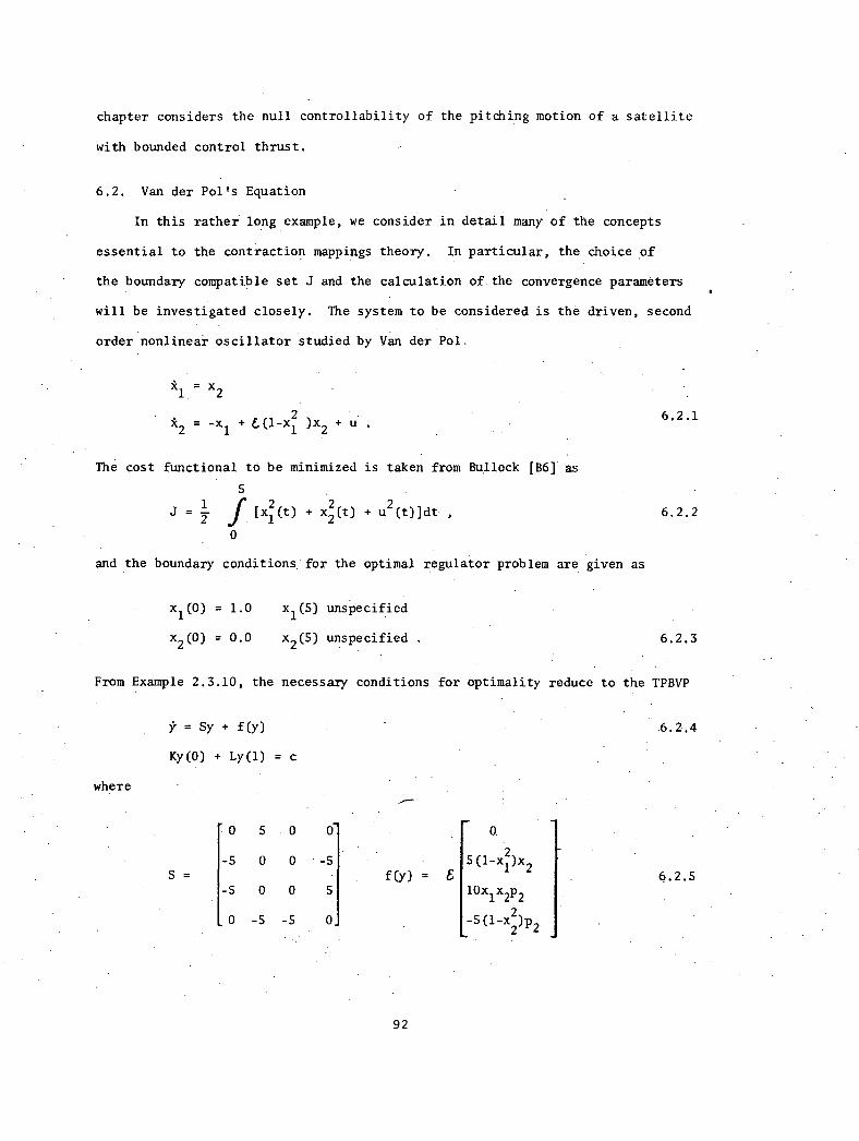
chapter considers the null controllability of the pitching motion of a satellite
with bounded control thrust.
6.2. Van der Pol's Equation
In this rather longexample, we consider in detail many of the concepts
essential to the contraction mappings theory. In particular, the choice of
the boundary compatible set J and the calculation of.the convergence parameters
will be investigated closely. The system to be considered is the driven, second
order nonlinear oscillator studied by Van der Pol.
k1 =x
2
k2 = -x
1 + E(1-x
1 )x2 + u .
The cost functional tO be minimized is taken from Bullock [B6] as
j21 2
+ x(t) + u2(t)]dt ,
and the boundary conditions for the optimal regulator problem are given as
x1(0) = 1.0 x1 (5) unspecified
x2(0) = 0.0 x2(5) unspecified .
6.2.1
6.2.2
6.2.3
From Example 2.3.10, the necessary conditions for optimality reduce to the TPBVP
= + f(y) 6.2.4
Ky(0) + Ly(1) = c
where
0 5 0 0 0
-5 0 0 -5 5(1-xl2 )x2
S = f(y) = 6 6.2.5-5 0 0 5 10x
1x2p2
_ 0 -5 -5 0, -5(1-x2
2)p2
92
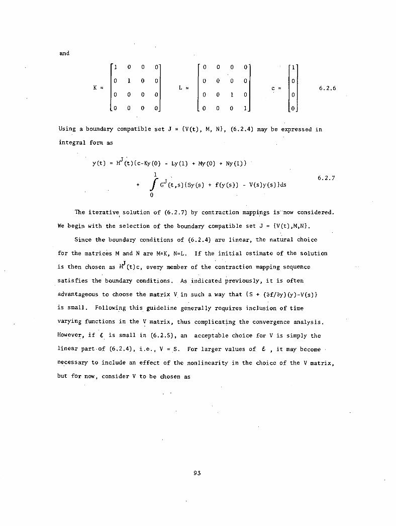
and
1 0 0 0 0 0 0 0 1
0 1 0 0 0 0 0 0K = L = C = 6.2.6
0 0 0 0 0 0 1 0 0
0 0 0 0 0 0 0 1_
Using a boundary compatible set J = {V(t), M, N}, (6.2.4) may be expressed in
integral form as
y(t) = Hj(t){c-Ky(0) - Ly(1) + My(0) + Ny(1)}
1
+ f ){sy(s) + f(y(s)) - v(s)y(s)}ds6.2.7
The iterative solution of (6.2.7) by contraction mappings is now considered.
We begin with the selection of the boundary compatible set J = {V(t),M,N}.
Since the boundary conditions of (6.2.4) are linear, the natural choice
for the matrices M and N are M=K, N=L. If the initial estimate of the solution
is then chosen as Hj(t)c, every member of the contraction mapping sequence
satisfies the boundary conditions. As indicated previously, it is often
advantageous to choose the matrix V in such a way that {S + (af/Dy)(y)-V(s)}
is small. Following this guideline generally requires inclusion of time
varying functions in the V matrix, thus complicating the convergence analysis.
However, if 6 is small in (6.2.5), an acceptable choice for V is simply the
linear part-of (6.2.4), i.e., V = S. For larger values of t , it may become
necessary to include an effect of the nonlinearity in the choice of the V matrix,
but for now, consider V to be chosen as
93
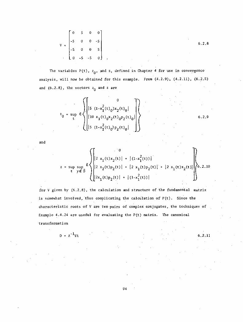
o s o
-5 0 0 -51.1
-5 0 0 5
_ 0 -5 -5 0
6.2.8
The variables P(t), zo, and z, defined in Chapter 4 for use in convergence
analysis, will now be obtained for this example. From (4.2.9), (4.2.11), (6.2.5)
and (6.2.8), the vectors z0 and z are
0
15 (1-xl2 (t)0)x2(t)0 1
z0
supt 110 x1(t)0x2(t)0p2(t)0 1
Is (1-xl2 (t)0)1)2(t)01
and
z = sup sup_t yE S
. '0
xl(t)x2(01 + 1(1-xf(t))1
2(t)p2(t)1 + 12 xl(t)p2(t)
(t)P2(01 1(1-4.(t))1
xl(t)x2(t)i
6.2.9
6.2.10
for V given by (6.2.8), the calculation and structure of the fundamental matrix
is sOmewhat involved, thus complicating the calcUlation of P(t). Since the
characteristic roots of V are two pairs of complex conjugates, the techniques of
Example 4.4.24 are useful for evaluating the P(t) matrix. The canonical
transformation
= A IVA
94
6.2;11
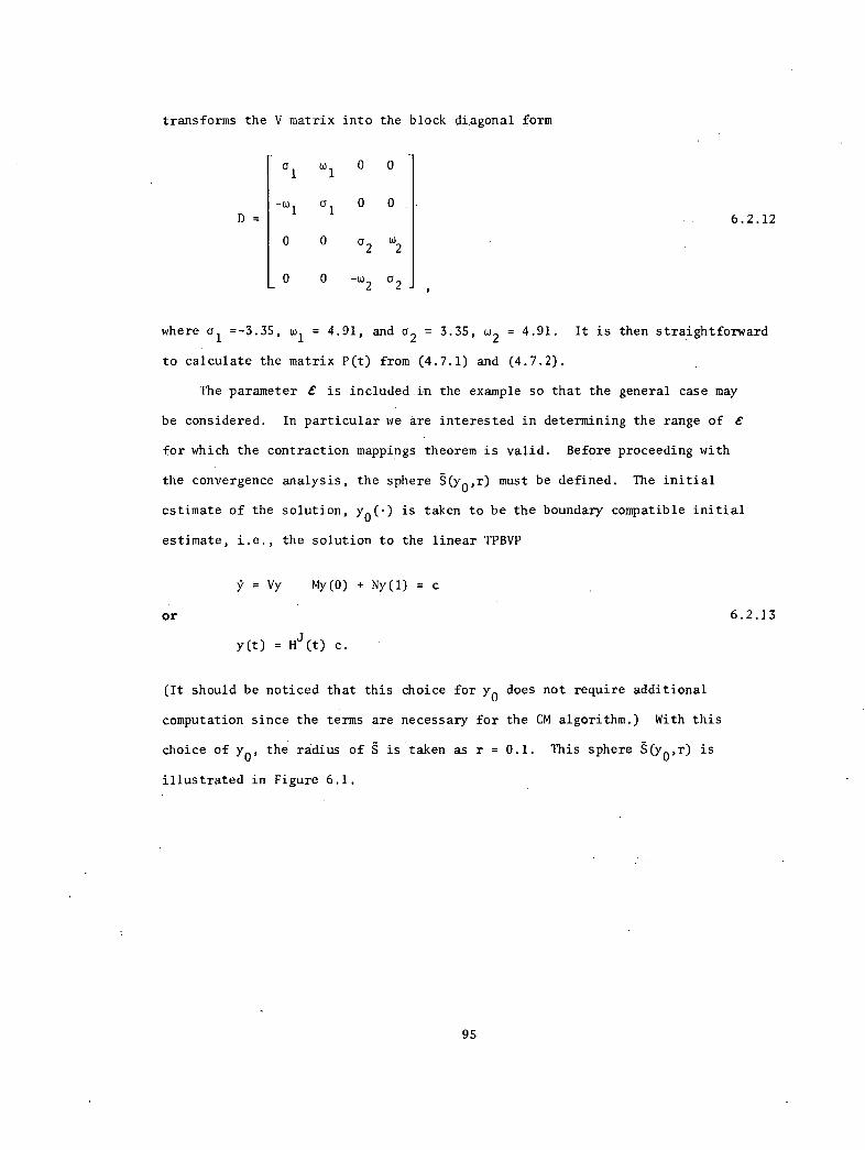
transforms the V matrix into the block diagonal form
a1
w1
0 0
D =-w
1a1
06.2.12
0 0 02 w2
_ 0 0 -w2
a2
where al =-3.35, wi = 4.91, and a2 = 3.35, w2 = 4.91. It is then straightforward
to calculate the matrix P(t) from (4.7.1) and (4.7.2).
The parameter e is included in the example so that the general case may
be considered. In particular we are interested in determining the range of C
for which the contraction mappings theorem is valid. Before proceeding with
the convergence analysis, the sphere g(yo,r) must be defined. The initial
estimate of the solution, yo(.) is taken to be the boundary compatible initial
estimate, i.e., the solution to the linear TPBVP
or
= Vy My(0) + Ny(1) = c
y(t) = Hjr(t) c.
6.2.13
(It should be noticed that this choice for yo does not require additional
computation since the terms are necessary for the CM algorithm.) With this
choice of yo, the radius of g is taken as r = 0.1. This sphere g(yo,r) is
illustrated in Figure 6.1.
95
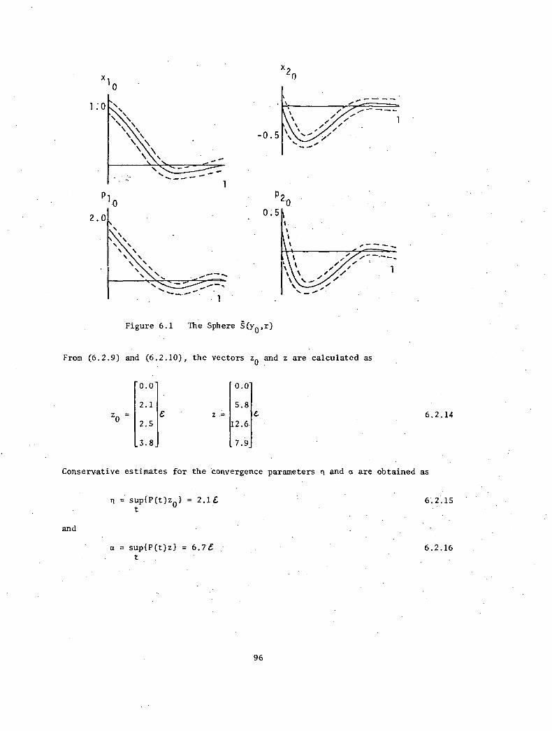
1
1:0
0
Figure 6.1
1
-0.5
P20
0:5
The Sphere (ycl,r)
••••.00
From (6.2.9) and (6.2.10), the vectors z0 and z are calculated as
z0
1
0.0- 0.0
2.1 5.8e z = 6 6.2.14
2.5 12.6
3.8 7.9
Conservative estimates for the convergence parameters n and a are obtained as
and
n = sup{P(t)z0} = 2.1 e 6.2.15t
a = sup{P(t)z} = 6.76 6.2.16t
96
Using (6.2.15) and (6.2.16), the requirements of Theorem 3.4.14 are specified as
and
6.7C < 1 6.2.17
2.1 C< 0.1
1-6.7E —6.2.18
Analysis of (6.2.17) and (6.2.18) shows that for 6 < 0.034 theconvergence
conditions of the theorem are satisfied.
The case for = 1.0 is treated in the paper "A Second-Order Feedback
Method for Optimal Control Computations", by Bullock and Franklin [B6]. In
the paper, the optimization problem presented by (6.1,2,3) is solved by the
techniques of steepest descent and second variation. We now consider the
application of contraction mappings to (6.2.4) with C = 1.0. Again the V matrix
is chosen V = S. Now rather than taking yo as the solution to the linear TPBVP,
y0(t) shall be given by the fifth iteration of the CM algorithm begun with the
initial guess Hj(t)c. This choice for yo is made so that the region Š(Y0,T) is
more likely to include the solution y(t) to the nonlinear TPBVP. We again take
r = 0.1. This sphere is illustrated in Figure 6.2.
We shall first determine the convergence rate factor a. Taking the supremum
over Š, z is given as
z =
97
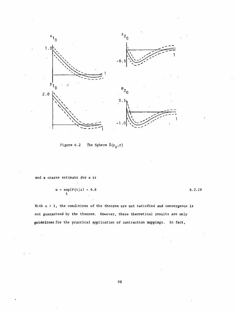
0
1.0
2.0
x20
-0.5
P20
Figure 6.2 The Sphere g(yo,r)
and a coarse estimate for a is
a = sup{P(t)z} = 6.8 6.2.19t
With a > 1, the conditions of the theorem are not satisfied and convergence is
not guaranteed by the theorem. However, these theoretical results are only
guidelines for the practical application of contraction mappings. In fact,
98
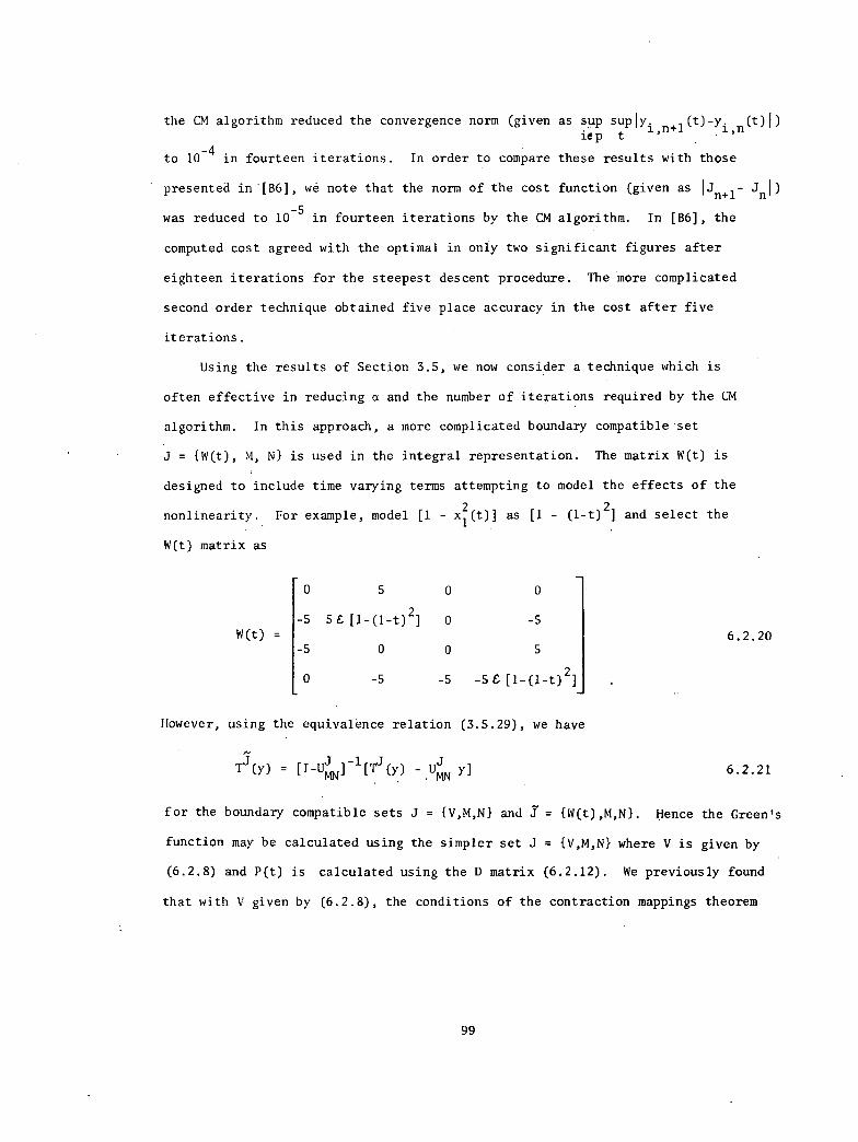
the CM algorithm reduced the convergence norm (given as sup suP1Yi n+1 (t) -Y-1 n (t )1), .,iep t
to 10 4
in fourteen iterations. In order to compare these results with those
presented in [86], we note that the norm of the cost function (given as 1J114.1
was reduced to 10-5
in fourteen iterations by the CM algorithm. In [B6], the
computed cost agreed with the optimal in only two significant figures after
eighteen iterations for the steepest descent procedure. The more complicated
second order technique obtained five place accuracy in the cost after five
iterations.
Using the results of Section 3.5, we now consider a technique which is
often effective in reducing a and the number of iterations required by the CM
algorithm. In this approach, a more complicated boundary compatible set
J = Mt), M, N} is used in the integral representation. The matrix W(t) is
designed to include time varying terms attempting to model the effects of the
nonlinearity. For example, model [1 - x12(t)] as [1 - (1-0
2] and select the
W(t) matrix as
0 5 0 0
-5 5 & [1-(1-t)2] 0 -5
-5 0 0 5
0 -5 -5 -5 E [1-(1-t)2]
However, using the equivalence relation (3.5.29), we have
W(t) =
J T3(y) = [I-U ]
-1 [1J
(y) - Uj
y]MN MN
6.2.20
6.2.21
for the boundary compatible sets J = {VAN} and = {W(OAN}. Hence the Green's
function may be calculated using the simpler set J = {V,M,N} where V is given by
(6.2.8) and P(t) is calculated using the D matrix (6.2.12). We previously found
that with V given by (6.2.8), the conditions of the contraction mappings theorem
99
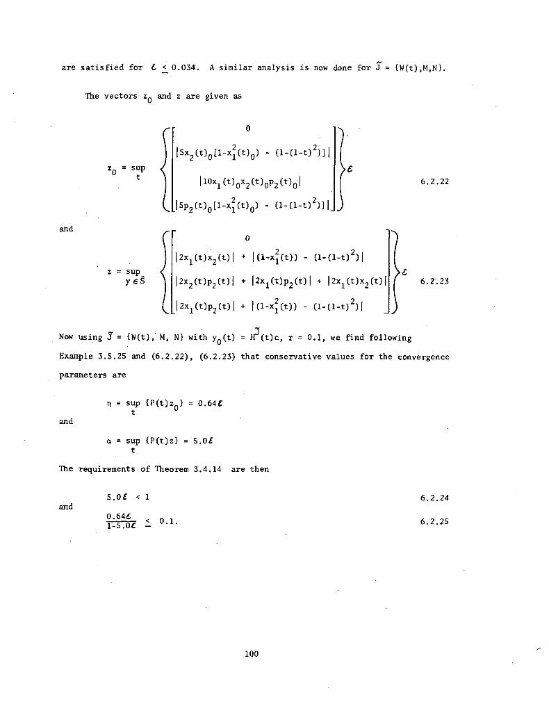
are satisfied for 6 < 0.034. A similar analysis is now
The vectors z0
and z are given as
0
done for .7= {w(t),m,N}.
15x2(t)
0[1-x
12 (t)
0) - (141-0
2
z0 = sup
t110x1(00x2W0p2(001{
15p2(t)0[1-x12 (00) - (1-(1-t)
2)]I_
6.2.22
and0
12x1(0x2(01 + 10-4(0) - (1-0-02)1
z = sup {yEs 1 2x2(0132(01 1 2x1(t)p2(t)1 + 12x1(t)x2(t)1
12x1(t)p2(t)1 + l(1-xf(t)) - (1-(1-t)2)1
6.2.23
Now using = {w(t), m, N} with yo(t) = 0(t)c, r = 0.1, we find following
Example 3.5.25 and (6.2.22), (6.2.23) that conservative values for the convergence
parameters are
and
n = sup {P(t)zio} = 0.64Ct
a = sup {P(t)z} = 5.OEt
The requirements of Theorem 3.4.14 are then
and5.0C < 1 6.2.24
0.64C 0.1. 6.2.251-5.0C —
100
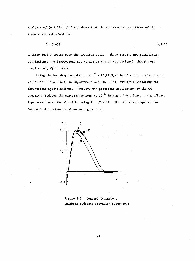
Analysis of (6.2.24), (6.2.25) shows that the convergence conditions of the
theorem are satisfied for
E< 0.092 6.2.26
a three fold increase over the previous value. These results are guidelines,
but indicate the improvement due to use of the better designed, though more
complicated, W(t) matrix.
Using the boundary compatible set 7 {W(t),M,N} for I = 1.0, a conservative
value for a is a = 5.1, an improvement over (6.2.14), but again violating the
theoretical specifications. However, the practical application of the CM
algorithm reduced the convergence norm to 10-5
in eight iterations, a significant
improvement over the algorithm using J = {V,M,N}. The iterative sequence for
the control function is shown in Figure 6.3.
Figure 6.3 Control Iterations
(Numbers indicate iteration sequence.)
101
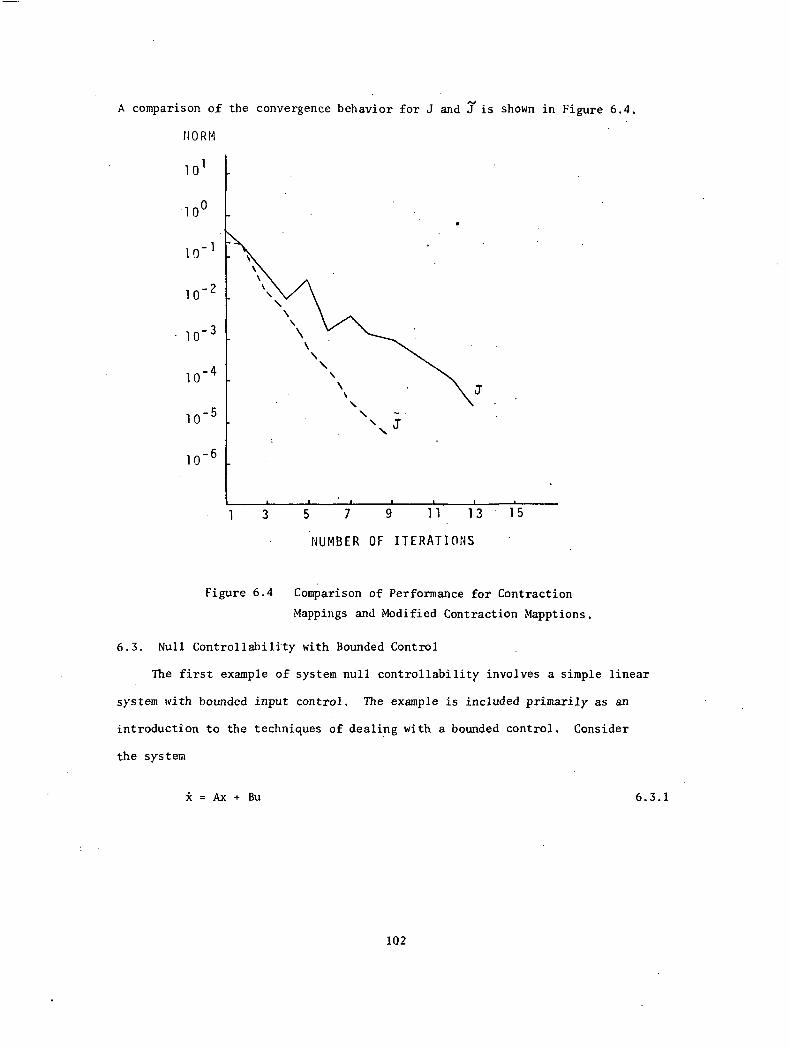
A comparison of the convergence behavior for J and Xis shown in Figure 6.4.
NORM
101
100
10
10-2
- 10-3
10-4
10-5
10-6
1 3 5 7 9 11'. 13 15
NUMBER OF ITERATIONS
Figure 6.4 Comparison of Performance for Contraction
Mappings and Modified Contraction Mapptions.
6.3. Null Controllability with Bounded Control
The first example of system null controllability involves a simple linear
system with bounded input control. The example is included primarily as an
introduction to the techniques of dealing with a bounded control. Consider
the system
= Ax + Bu 6.3.1
102
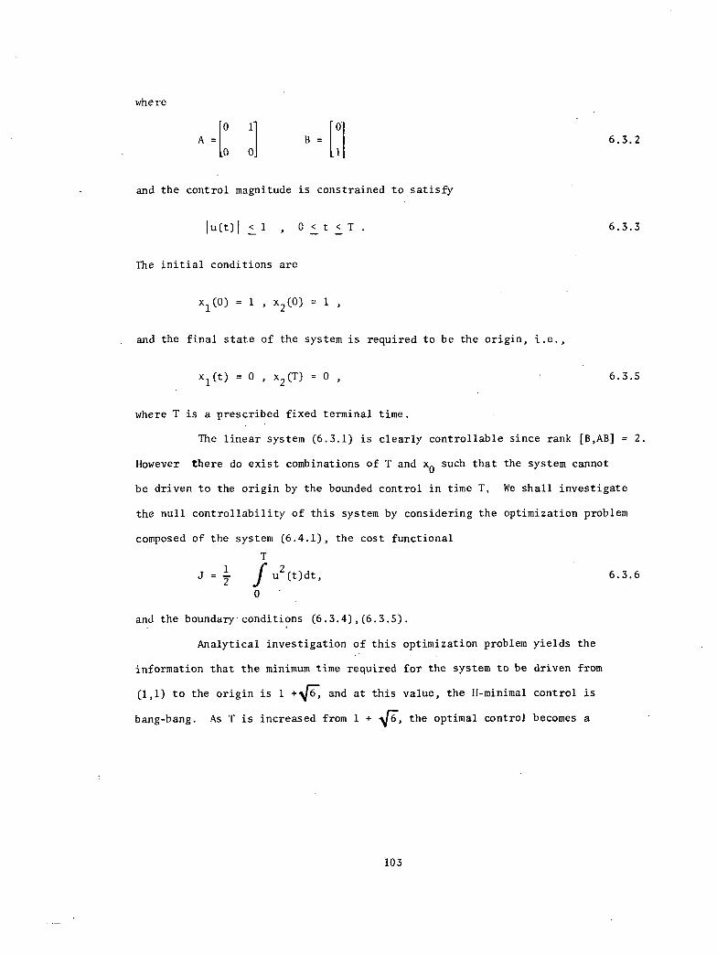
where
A=10 1
1 0 0B =
[O16.3.2
and the control magnitude is constrained to.satisfy
lu(t) < 1 , 0 < t < T . 6.3.3
The initial conditions are
x1(0) = 1 , x2(0) = 1 ,
and the final state of the system is required to be the origin, i.e.,
xl(t) = 0 , x2(T) = 0 , 6.3.5
where T is a prescribed fixed terminal time.
The linear system (6.3.1) is clearly controllable since rank [B,AB] = 2.
However there do exist combinations of T and x0
such that the system cannot
be driven to the origin by the bounded control in time T, We shall investigate
the null controllability of this system by considering the optimization problem
composed of the system (6.4.1), the cost functional
T
J = 2 f u2 (t)dt, 6.3.6
0
and the boundary conditions (6.3.4),(6.3.5).
Analytical investigation of this optimization problem yields the
information that the minimum time required for the system to be driven from
(1,1) to the origin is 1 +47, and at this value, the H-minimal control is
bang-bang. As T is increased from 1 + 4T, the optimal control becomes a
103
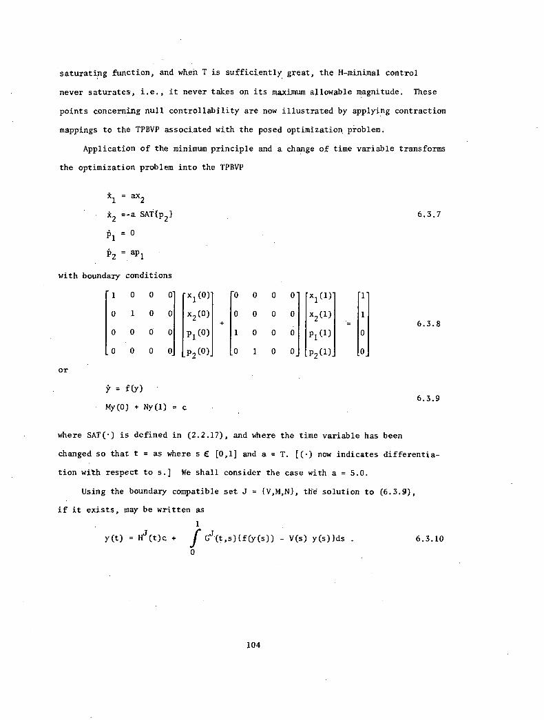
saturating function, and when T is sufficiently great, the H-minimal control
never saturates, i.e., it never takes on its maximum allowable magnitude. These
points concerning null controllability are now illustrated by applying contraction
mappings to the TPBVP associated with the posed optimization. pioblem.
Application of the minimum principle and a change of time variable transforms
the optimization problem into the TPBVP
ax21
i2 =-a SAT{p2} 6.3.7
1)1 = 0
P2 =ap1
with boundary conditions
1 0 0 0-xl(0)
0 0 0 0 x1(1)- 1
0 1 0x2(0)
0000 x2(1) 16.3.8
0000 p1(0) 1000 p1(1)0000
P2(0)-0 1 0 0_ 132(1)- o_
or
= f(y)6.3.9
• My(0) + Ny(1) = c
where SAT(•) is defined in (2.2.17), and where the time variable has been
changed so that t = as where s E [0,1] and a = T. [(.) now indicates differentia-
tion with respect to s.] We shall consider the case with a = 5.0.
Using the boundary compatible set J = {VAN}, the solution to (6.3.9),
if it exists, may be written as
1
y(t) = Hj(t)c + j(- Gj(t,$){f(y(s)) - V(s) y(s)}ds .
0
104
6.3.10
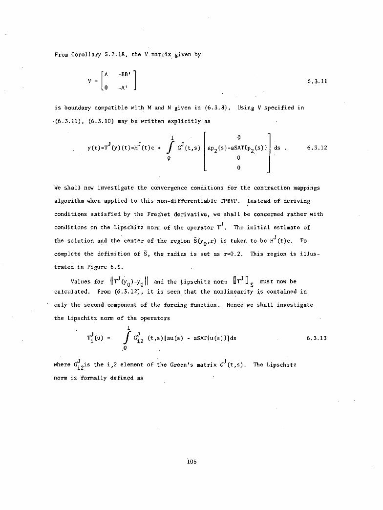
From Corollary 5.2.18, the V matrix given by
A -BP]V = 6.3.11
0 -A'
is boundary compatible with M and N given in (6.3.8). Using V specified in
(6.3.11), (6.3.10) may be written explicitly as
1 0
y(t)=Tj(y)(t)=Hj(t)c + J Gj(t,$) ap2(s)-aSAT{p2(s)} ds . 6.3.12
0
0
We shall now investigate the convergence conditions for the contraction mappings
algorithm when applied to this non-differentiable TPBVP. Instead of deriving
conditions satisfied by the Frechet derivative, we shall be concerned rather with
conditions on the Lipschitz norm of the operator Tj. The initial estimate of
the solution and the center of the region (yo,r) is taken to be Hj(t)c. To
complete the definition of Š, the radius is set as r=0.2. This region is illus-
trated in Figure 6.5.
Values for HTJ (y0)-yo ll and the Lipschitz norm OTj 0- must now be
calculated. From (6.3.12), it is seenthat the nonlinearity is contained in
only the second component of the forcing function. Hence we shall investigate
the Lipschitz norm of the operators
1
Ti(u) =i2 (t,$)[au(s) - aSAT{u(s)}]ds
0
where Gi2is the i,2 element of the Green's matrix GJ (t,$). The Lipschitz
norm is formally definod as
105
6.3.13
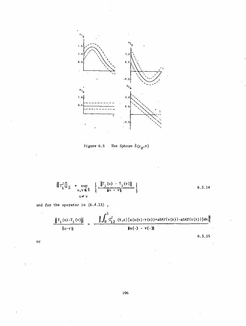
'20
p10
1.0
0 5
Figure 6.5 The Sphere g (y0 ,r)
IITI = sup_ liTi (u) - Ti (v)ll
u v E S - v 11S 6.3.14
,
v
and for the operator in (6.4.13) ,
OT
1
Ti (u)-Ti (v)11 fo Gji2 (t,$) [a(u (s )-v (s) )+aSAT{v (s ) }-aSAT{u (s) }jds
llu-v Hu(*) - v(.)11
106
6.3.15
hTi(u)-Ti (11Hu - vH
Now noting
1
a sup fIG1 (t,$){[u(s),v(s))4[SAT{v(s)}-SAT{u(s)}1}Ids< t 0
sup lu(P)-v(P)
sisiplu(p)-v(P)1 > lu(s)-v(s)1
and
we have
suplu(P)-v(P)1 > ISAT{u(s)}-SAT {v(s)}1
ri(u)-Ti(v)I1
Hu -
6.3.16
6.3.17
6.3.18
1
a sup flG
(t,s u(s)-v(s) SAT{v(s)}-SAT{u(s)}
Ids12 lu(š)-v(S)1 lu(s)-v(s)[0
It may be shown that with r = 0.2
I u(s)-v(s) SAT{v(s)}-SAT{u(s)} < 2
lu(s)-v(s)1 u(s)-v(s)
6.3.19
6.3.20
The required Lipschitz norm may now be evaluated in several ways, each of varying
degrees of accuracy. We now consider one of the more accurate techniques.
Note that as a result of the choice of (yo,r), saturation can only occur
for 0 < s < 0.25. We may now write
ri(u)—Ti(v)11
nu —
.25
<2asuplf1.G12
(t,$)Idst 0
which may be approximated as
107
6.3.21
where
Pag<supsup{2a(.25).P12(t)} = 5/16 < 1
i t
.11. (t) = IGj (t s)lds .P12 Gj (t s)lds +
II. 'Ii,2 1,2
0
Now determining 11Tj (y0) - y0 11 , we have
From yo(*)
and then
6.3.22
6.3.23
1Ti(y0) - yoi Gi2(t,$)[ap2(s)0 - aSAT{p2(s)0}]ds 6.3.24
sup{lap2(00 - aSAT{p2(t)0}1) < 0.04a , 6.3.25t
ITJ(Y0)-4.25
_ . 1< sup sup{0.04a 1G.
2 (t' s)ids}
i t 0
< (0.04a)(0.25)sup sup {Pi2(t)} = 60 '
i t
Taking conservative values a = 5/16, n = 1/60 ,
= 0.1 < r = 0.2
so that the theoretical application of contraction mappings is successful.
Hence a solution exists to the TPBVP and a control exists to accomplish the
desired transfer. These concepts will now be applied to a nonlinear system.
108
6.3.26
6.3.27
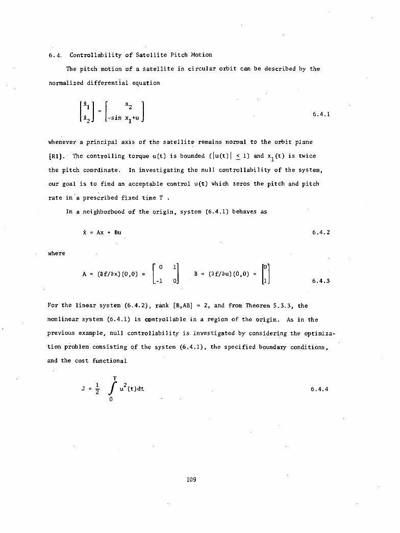
6.4. Controllability of Satellite Pitch Motion
The pitch motion of a satellite in circular orbit can be described by the
normalized differential equation
xl x2
=x2
-sin x1+u
6.4.1
whenever a principal axis of the satellite remains normal to the orbit plane
[R1]. The controlling torque u(t) is bounded (lu(t)1 1) and xl(t) is twice
the pitch coordinate. In investigating the null controllability of the system,
our goal is to find an acceptable control u(t) which zeros the pitch and pitch
rate in a prescribed fixed time T
In a neighborhood of the origin, system (6.4.1) behaves as
where
= Ax + Bu 6.4.2
A = (af/3x)(0,0) =-1 0
B = (3f/au)(0,0) =6.4.3
For the linear system (6.4.2), rank [B,AB] = 2, and from Theorem 5.3.3, the
nonlinear system (6.4.1) is cnntrollable in a region of the origin. As in the
previous example, null controllability is investigated by considering the optimiza-
tion problem consisting of the system (6.4.1), the specified boundary conditions,
and the cost functional
1J =
2 — f
u2 (t)dt
0
109
6.4.4
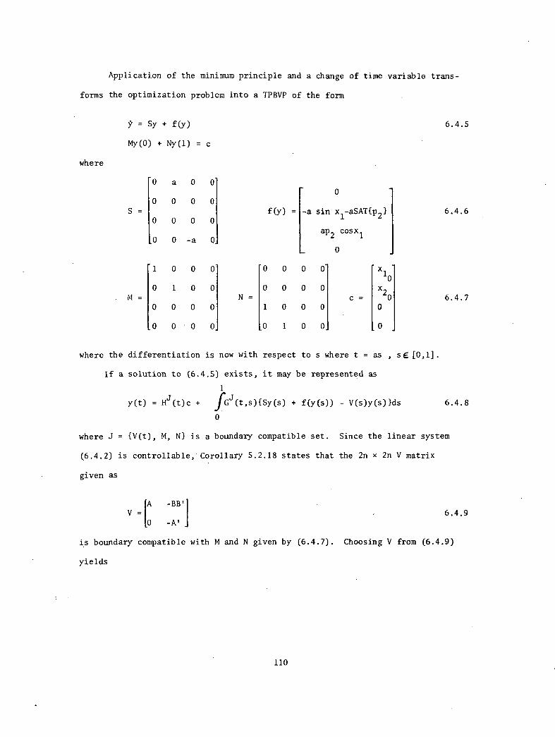
Application of the minimum principle and a change of time variable trans-
forms the optimization problem into a TPBVP of the form
= Sy + f(y)
My(0) + Ny(1) = c
where
6.4.5
0 a 0 00
0 0 0 0S = f(y) = -a sin xl-aSAT{p2} 6.4.6
0 0 0 0ap2 cosx1
0 0 -a 00
1 0 0 0 0 0 0 0 x10
0 1 0 0 0 0 0 0 x2
M = N = c = 0 6.4.70 0 0 0 1 0 0 0
0 0 0 0 0 1 0 0 0
where the differentiation is now with respect to s where t = as , sE [0,1].
If a solution to (6.4.5) exists, it may be represented as
1
y(t) = Hj(t)c + j(P(t,$){Sy(s) + f(y(s)) - V(s)y(s)}ds 6.4.8
0
where J = {V(t), M, N} is a boundary compatible set. Since the linear system
(6.4.2) is controllable, Corollary 5.2.18 states that the 2n x 2n V matrix
given as
A -BB'lV =
0 -A'6.4.9
is boundary compatible with M and N given by (6.4.7). Choosing V from (6.4.9)
yields
110
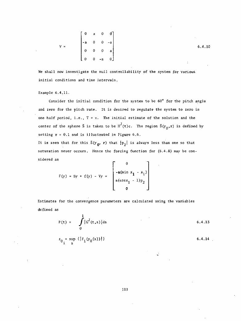
0 a 0 6-
-a 0 0 -aV = 6.4.10
0 0 0 a
0 0 -a 0
We shall now investigate the null controllability of the system for various
initial conditions and time intervals.
Example 6.4.11.
Consider the initial condition for the system to be 60° for the pitch angle
and zero for the pitch rate. It is desired to regulate the system to zero in
one half period, i.e., T = IT. The initial estimate of the solution and the
center of the sphere S is taken to be Hj(t)c. The region g(yo,r) is defined by
setting r = 0.1 and is illustrated in Figure 6.6.
It is seen that for this 8(yo, r) that Ip2 1 is always less than one so that
saturation never occurs. Hence the forcing function for (6.4.8) may be con-
sidered as
F(y) = Sy + f(y) - Vy =
0
-a(sin
a(cosx1
0
Estimates for the convergence parameters are calculated using the variables
defined as
1
P(t) = fle(t,$)Ids
0
6.4.13
z0 = sup {1Fi(y0(s))1) 6.4.14
s
111
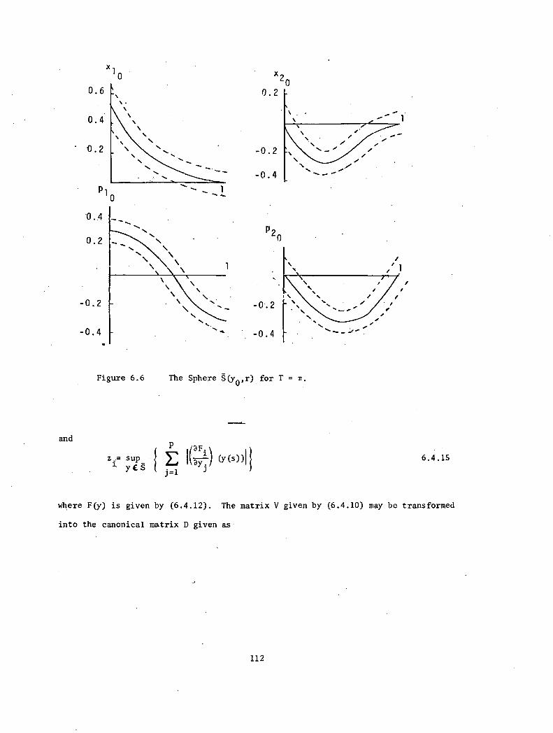
and
O. 4
0.2
-0 . 2
-0 . 4
1120
1
•
_ -0 . 2
-0 . 4
\
•\
•
Figure 6.6 The Sphere g(yo,r) for T = n.
P i(aFiz ;.= sup_ / E 1 ,77-) (y(s))11
y S j=1 dYj
6.4.15
where F(y) is given by (6.4.12). The matrix V given by (6.4.10) may be transformed
into the canonical matrix D given as
112
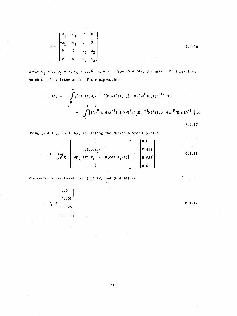
O
D =- wl 1
O O6.4.16
0 0a2 w2
0 0 -w2
a2
where al = 0, wl = a, a2 = 0.05, w2 = a. From (6.4.14), the matrix P(t) may then
be obtained by integration of the expression
P(t) = j6{A0(t,O)A-1
}([M+N(Dv(1,0)]-1
M}{114)D(0,$)A
-1}Ids
0
jr1{A0 (t,O)A-1}{[M+NOV(1,0)]-1NOV(1,0)}{A0(0,$)A-1}1ds
6.4.17
Using (6.4.12), (6.4.15), and taking the supremum over S yields
0 0.0
la(cosx1-1)1 0.418z = sup_
=
6.4.18yE S lap2 sin x1 l + la(cos x1-1)I 0.653
0 0.0
The vector z0 is found from (6.4.12) and (6.4.14) as
-0.0
0.095z0
6.4.190.028
_0.0
113
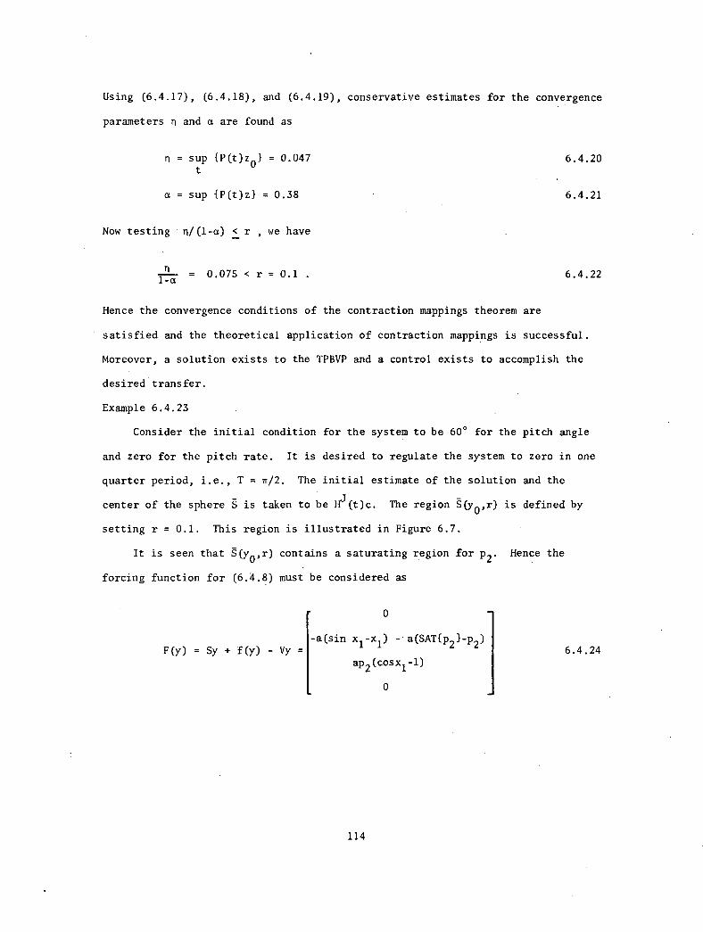
Using (6.4.17), (6.4.18), and (6.4.19), conservative estimates for the convergence
parameters n and a are found as
n = sup {P(t)z0} = 0.047 6.4.20t
a = sup {P(t)z} = 0.38 6.4.21
Now testing n/(1-a) < r , we have
ri1-a
= 0.075 < r = 0.1 . 6.4.22
Hence the convergence conditions of the contraction mappings theorem are
satisfied and the theoretical application of contraction mappings is successful.
Moreover, a solution exists to the TPBVP and a control exists to accomplish the
desired transfer.
Example 6.4.23
Consider the initial condition for the system to be 60° for the pitch angle
and zero for the pitch rate. It is desired to regulate the system to zero in one
quarter period, i.e., T= n/2. The initial estimate of the solution and the
center of the sphere S is taken to be Hj(t)c. The region kyo,r) is defined by
setting r = 0.1. This region is illustrated in Figure 6.7.
It is seen that g(yo,r) contains a saturating region for p2. Hence the
forcing function for (6.4.8) must be considered as
F(y) = Sy + f(y) - Vy =
0
-a(sin xl-x1) - a(SAT{p2}-p2)
ap2(c osx
1 -1)
0
114
6.4.24
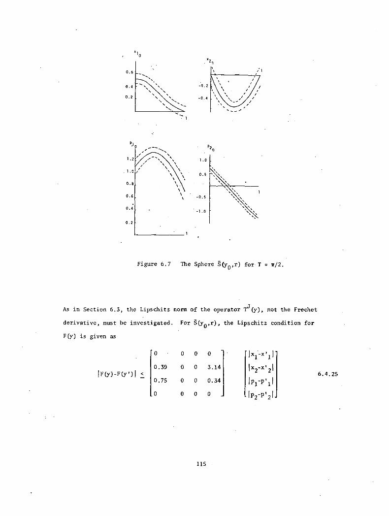
0.6
0.4
0.2
1.2
1.0
0.8
0.6
0.4
0.2
1.0
0.5
-0.5
-1.0
P20
Figure 6.7 The Sphere g(yo,r) for. T = w/2.
As in Section 6.3, the Lipschitz norm of the operator Tj(y), not the Frechet
derivative, must be investigated. For g(yo,r), the Lipschitz condition for
F(y) is given as
IF(y)-F(>")1 <
0
0.39
0.75
0
0 0 0 - -jx1.-)01 1
0 0 3.14 Ix2-x'210 0 0.34 Ipl-p'1 10 0 0 Ip2-p'2 1 -
115
6.4.25
or
IIF(y) - F6r911 < C Ily - II • 6.4.26
Using P(t) from (6.4.17) and defining the 2n vector z as composed of the elements
2n
jzi = 2: [C
ij , 6.4.27
j=1
a conservative estimate for a is UP(.)z11 . However, because the saturation
occurs only over a short interval of .(y(:), r) , this estimate would tend to be
quite inaccurate. Hence we deal with the saturation effect separately. Now let
0 0
0.34 3.14=
1 1.14and z
2 =
06.4.28
0 0
where z1
arises from the differentiable part and z2
from the saturating effect.
Then as in Section 6.3 ,
or
1.0
a = sup {P(t)21} + sup I f G (t,$)z2Ids
0,85
6.4.29
a = sup {P(t)z1} + sup{(3.14)(0.15)Pi2(t)} . 6.4.30
Using the values of P(t) from (6.4.17), a is evaluated as
a = 1.56 . 6.4.31
116
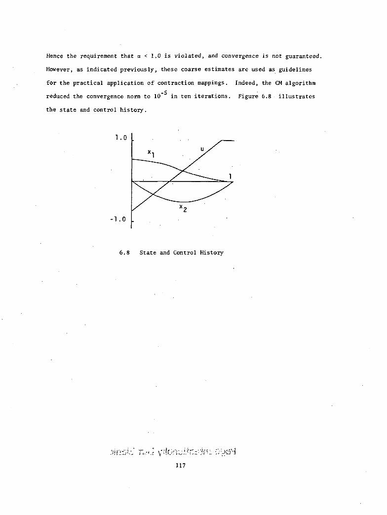
Hence the requirement that a < 1.0 is violated, and convergence is not guaranteed.
However, as indicated previously, these coarse estimates are used as guidelines
for the practical application of contraction mappings. Indeed, the CM algorithm
reduced the convergence norm to 10-5
in ten iterations. Figure 6.8 illustrates
the state and control history.
1 .0
- 1 .0
6.8 State and Control History
L
117

Page Intentionally Left Blank
CHAPTER 7
PRELIMINARY STUDY ON THE DYNAMICS OF
DRUG USAGE WITHIN A COMMUNITY
7.1. Introduction
The modeling of complex socio-economic systems has recently received con-
siderable attention. Arising initially as an aid to management decision making,
[F7], [R2], system modeling is now applied to many systems of public concern
[F5], [R3]. The primary objective of the modeling effort is the formulation of
improved administrative control policies. Typically, once a model is developed,
the process of designing improved policies is largely a trial and error process.
That is, the behavior of the system is first simulated with the model using one
control policy and then another. The simulation results are then compared to
determine which policy yielded the "best" behavior, clearly an inexact and
inefficient technique of analysis.
In this chapter we consider the feasibility of applying the systematic
techniques of optimal control theory to the determination of policies for
social systems. Specifically, a dynamic model attempting to represent the
causal, feedback structure of community drug usage is developed. Then using
optimization theory, we attempt to gain insight into how a community might best
respond to a rapidly growing heroin addiction problem. The initial phase of
the study is the creation of a dynamic model which reflects the modes of behavior
of the system being investigated.
119
7.2. Development of a Dynamic Model
The development of a model for a complex system such as drug usage is in
itself a major effort. The subtle interrelationships and multi-feedback loops
are often difficult to conceptualize. Likewise, the determination of various
parameters within the model is a difficult task involving much data analysis.
The main thrust of this chapter is not in the modeling direction. Rather, we
shall develop a simple model which hopefully reflects inpart the basic behavior
of a yery complex system. Similarly, parameter values are chosen after discussions
and readings and are believed to be reasonable. In this spirit, the development
of the model is begun. (For the development of a more comprehensive model,
see Roberts [R3]).
The model concerns itself with three groups of people within the community.
These groups represent the three levels of drug usage which will be considered in
the model. These three pools of people are:
i) potential drug users
ii) drug users
iii) heroin addicts
'Of course, much finer lines may be drawn, but these three are sufficient for this
study. The dynamical nature of this problem is refiected in the constantly
changing population of each level and the inherent relationships between these
changes. The multiple interrelationships are often difficultto conceptualize,
but are critical to the feedback, multiloop structure of the system. Figure 7..1
represents how one might initially conceive this system as simply involving
transitions of people from various stages of drug usage.
In Figure 7.1, the double lines represent the flow of people between levels and
the values controiling these flows are determined by the variables alongside.
120
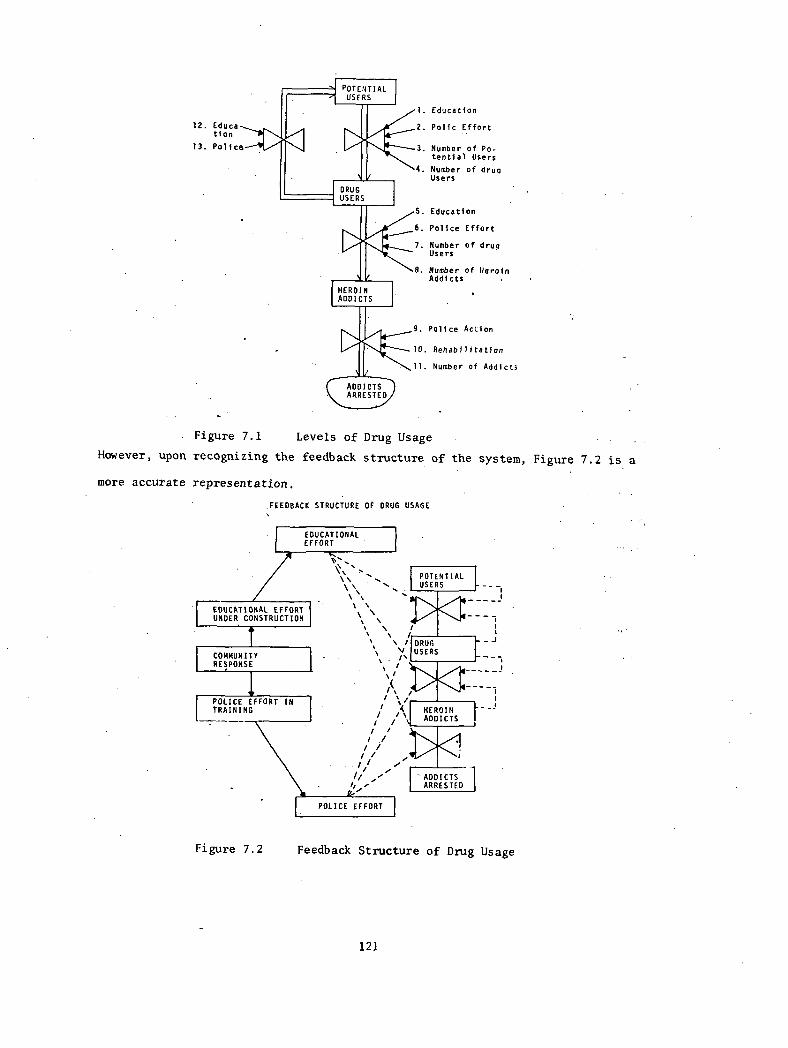
12. Educa--.,__tion
13. Police---.
POTENTIALUSERS
DRUGUSERS
/
HERO NADDICTS
1. Education
2. Polic Effort
Number of Po-tential Users
4. Number of drugUsers
5. Education
6. Police Effort
7. Number of drugUsers
8. Number of HeroinAddicts
9. Police Action4------
• 10. Rehabilitation
11. Number of Addicts
ADDICTS)ARRESTED
Figure 7.1 Levels of Drug Usage
However, upon recognizing the feedback structure of the system, Figure 7.2 is a
more accurate representation.
,FEEDRACK STRUCTURE OF DRUG USAGE
EDUCATIONALEFFORT
r-EDUCATIONAL EFFORTUNDER CONSTRUCTION
COMMUNITYRESPONSE
I POLICE EFFORT INTRAINING
POLICE EFFORT
POTENTIALUSERS
DRUGUSERS
HEROINADDICTS
'ADDICTSARRESTED
Figure 7.2 Feedback Structure of Drug Usage
121
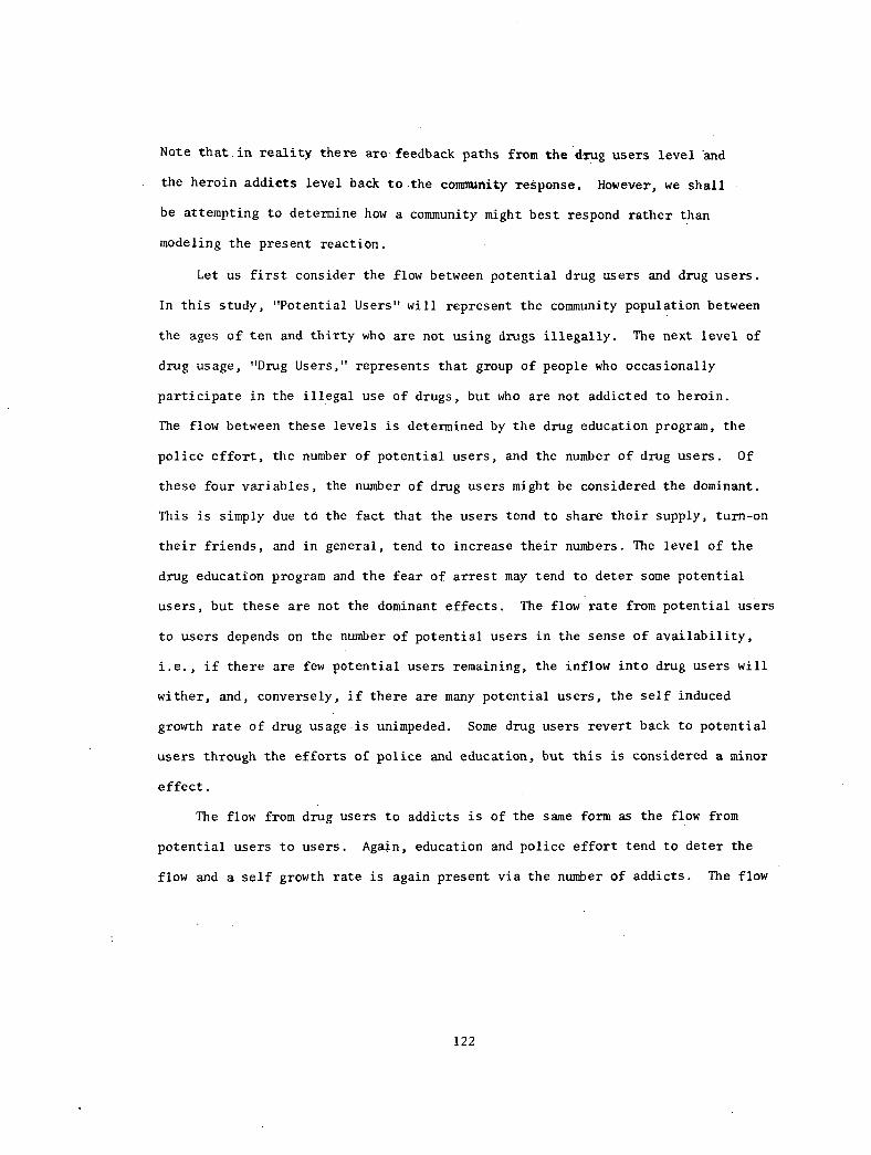
Note that in reality there are feedback paths from the drug users level -and
the heroin addicts level back to the community response, However, we shall
be attempting to determine how a community might best respond rather than
modeling the present reaction.
Let us first consider the flow between potential drug users and drug users.
In this study, "Potential Users" will represent the community population between
the ages of ten and thirty who are not using drugs illegally. The next level of
drug usage, "Drug Users," represents that group of people who occasionally
participate in the illegal use of drugs, but who are not addicted to heroin.
The flow between these levels is determined by the drug education program, the
police effort, the number of potential users, and the number of drug users. Of
these four variables, the number of drug users might be considered the dominant.
This is simply due to the fact that the users tend to share their supply, turn-on
their friends, and in general, tend to increase their numbers. The level of the
drug education program and the fear of arrest may tend to deter some potential
users, but these are not the dominant effects. The flow rate from potential users
to users depends on the number of potential users in the sense of availability,
i.e., if there are few potential users remaining, the inflow into drug users will
wither, and, conversely, if there are many potential users, the self induced
growth rate of drug usage is unimpeded. Some drug users revert back to potential
users through the efforts of police and education, but this is considered a minor
effect.
The flow from drug users to addicts is of the same form as the flow from
potential users to users. Again, education and police effort tend to deter the
flow and a self growth rate is again present via the number of addicts. The flow
122
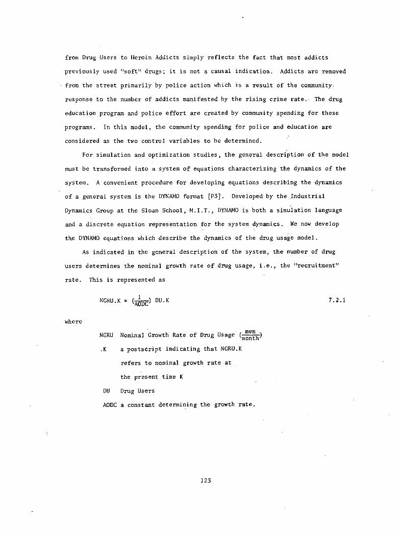
from Drug Users to Heroin Addicts simply reflects the fact that most addicts
previously used "soft" drugs; it is not a causal indication. Addicts are removed
from the street primarily by police action which is a result of the community
response to the number of addicts manifested by the rising crime rate.. The drug
education program and police effort are created by community spending for these
programs. In this model, the community spending for police and education are
considered as the two control variables to be determined.
For simulation and optimization studies, the general description of the model
must be transformed into a system of equations characterizing the dynamics of the
system. A convenient procedure for developing equations describing the dynamics
of a general system is the DYNAMO format [P3]. Developed by the Industrial
Dynamics Group at the Sloan School, M.I.T., DYNAMO is both a simulation language
and a discrete equation representation for the system dynamics. We now develop
the DYNAMO equations which describe the dynamics of the drug usage model.
As indicated in the general description of the system, the number of drug
users determines the nominal growth rate of drug usage, i.e., the "recruitment"
rate. This is represented as
where
NGRU.K - (AODC-) DU.K
-
1NGRU Nominal Growth Rate of Drug Usage (
mennonth'
.K a postscript indicating that NGRU.K
refers to nominal growth rate at
the present time K
DU Drug Users
AODC a constant determining the growth rate.
123
7.2.1
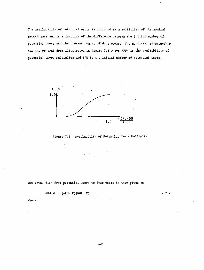
The availability of potential users is included as a multiplier of the nominal
growth rate and is a function of the difference between the initial number of
potential users and the present number of drug users. The nonlinear relationship
has the general form illustrated in Figure 7.3 where APUM is the availability of
potential users multiplier and IPU is the initial number of potential users.
APUM
1.0
1.0IPU-DUIPU
Figure 7.3 Availability of Potential Users Multiplier
The total flow from potential users to drug users is then given as
where
GRU.KL = (APUM.K)(NGRU.K) 7.2.2
124
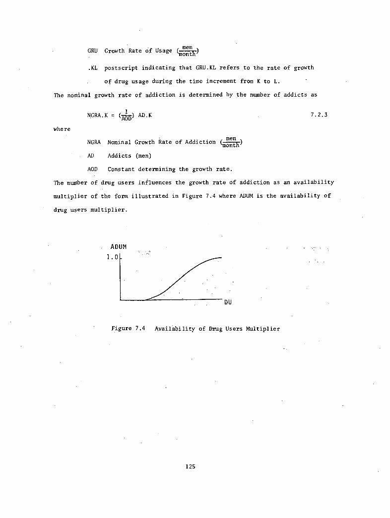
1GRU Growth Rate of Usage (
men-month'
.KL postscript indicating that GRU.KL refers to the rate of growth
of drug usage during the time increment from K to L.
The nominal growth rate of addiction is determined by the number of addicts as
where
NGRA.K = (Ta)
AD.K
1NGRA
4 Nominal Growth Rate of Addiction
menrcfEnoi j
AD Addicts (men)
7.2.3
AOD Constant determining the growth rate.
The number of drug users influences the growth rate of addiction as an availability
multiplier of the form illustrated in Figure 7.4 where ADUM is the availability of
drug users multiplier.
ADUM
1.0
DU
Figure 7.4 Availability of Drug Users Multiplier
125
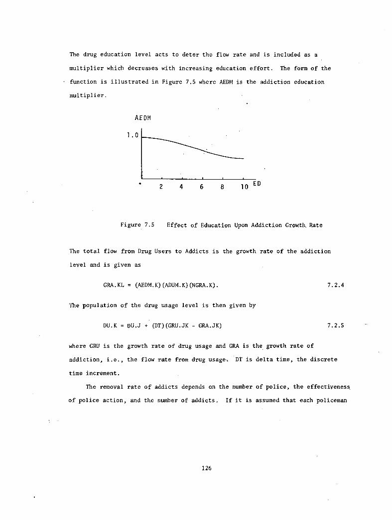
The drug education level acts to deter the flow rate and is included as a
multiplier which decreases with increasing education effort. The form of the
• function is illustrated in Figure 7.5 where AEDM is the addiction education
multiplier.
AEDM
1.0
2 4 6 8 10 ED
Figure 7.5 Effect of Education Upon Addiction Growth Rate
The total flow from Drug Users to Addicts is the growth rate of the addiction
level and is given as
GRA.KL = (AEDM.K)(ADUM.K)(NGRA.K).
The population of the drug usage level is then given by
DU.K = DU.J + (DT)(GRU.JK - GRA.JK)
where GRU is the growth rate of drug usage and GRA is the growth rate of
7.2.4
7.2.5
addiction, i.e., the flow rate from drug usage: DT is delta time, the discrete
time increment.
The removal rate of addicts depends on the number of police, the effectiveness
of police action, and the number of addicts. If it is assumed that each policeman
126
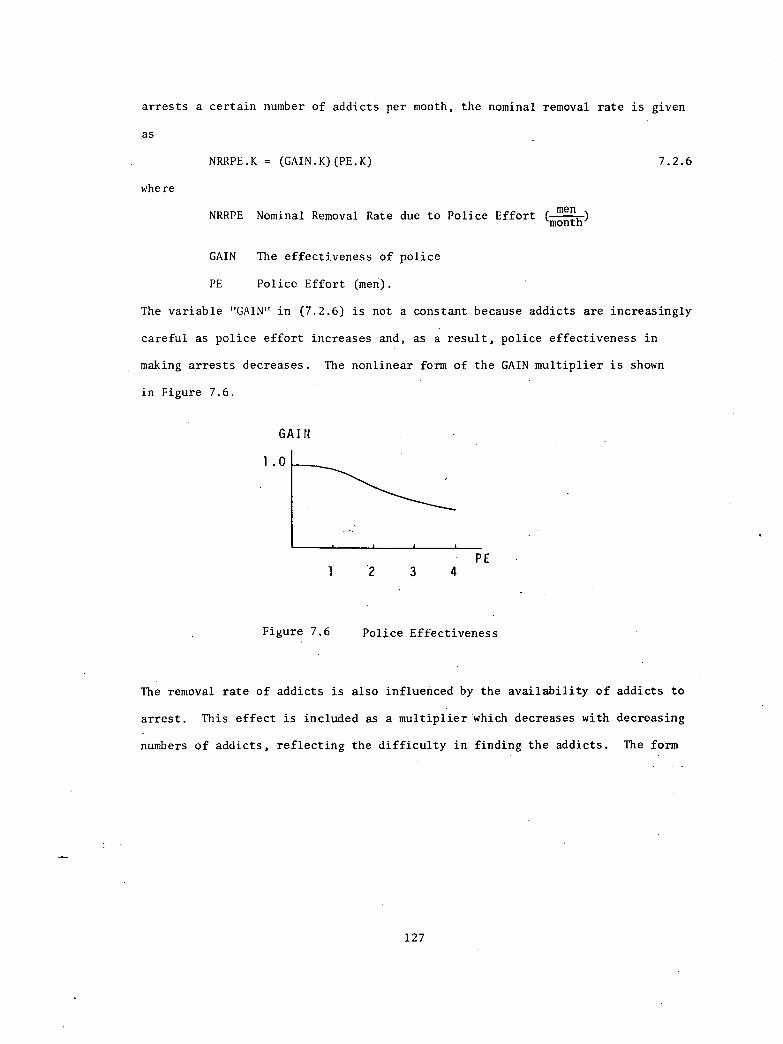
arrests a certain number of addicts per month, the nominal removal rate is given
as
where
NRRPE.K = (GAIN.K)(PE.K) 7.2.6
,NRRPE Nominal Removal Rate due to Police Effort (
men-month'
GAIN The effectiveness of police
PE Police Effort (men).
The variable "GAIN" in (7.2.6) is not a constant because addicts are increasingly
careful as police effort increases and, as a result, police effectiveness in
making arrests decreases. The nonlinear form of the GAIN multiplier is shown
in Figure 7.6.
GAIN
1.0
1 2 3 4
Figure 7.6
PE
Police Effectiveness
The removal rate of addicts is also influenced by the availability of addicts to
arrest. This effect is included as a multiplier which decreases with decreasing
numbers of addicts, reflecting the difficulty in finding the addicts. The form
127
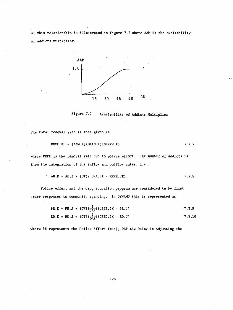
of this relationship is illustrated in Figure 7.7 where AAM is the availability
of addicts multiplier.
AAM
1.0
Figure 7.7
15 30 45 60AD
Availability of Addicts Multiplier
The total removal rate is then given as
RRPE.KL = (AAM.K)(GAIN.K)(NRRPE.K) 7.2.7
where RRPE is the removal rate due to pOlice effort. The number of addicts is
then the integration of the inflow and outflow rates, i.e.,
AD.K = AD.J + (DT)( GRA.JK RRPE.JK). 7.2.8
Police effort and the drug education program are considered to be.first
order responses to community spending. In DYNAMO this is represented as
PE.K = PE.J + (DT)(1757)(CSPE.JK - PE.J)
ED.K = ED.J + (DT)(---)(CSED.JK - ED.J)DAE
where PE represents the Police Effort (men), DAP the Delay in Adjusting the
128
7.2.9
7.2.10
ii) Police:
Police (months), CSPE the Community Spending on Police Effort (men), CSPE the
Community Spending on Police Effort (men), ED the Education program (men), DAP
the Delay in Adjusting the Education program (months), and CSED the Community
Spending on Education (men).
This completes the development of the system equations, however a simplifica-
tion is now considered. The three states "Potential Users", "Drug Users", and
"Heroin Addicts" are included in the model equations. These three states modeled
the changing population for three divisions of the youth population. However,
in many communities, especially those in which heroin addiction is becoming a
problem, the time dynamics of the first two variables have been completed. That
is, the percentage of the youth population which falls into the extremely broad
category "Drug Users" is relatively fixed or slowly time varying, the major
growth phase being essentially complete. For these reasons, only the variable
"Heroin Addicts" is included as a dynamic variable. This assumption yields the
following equations describing the system:
i) Addicts: AD.K = AD.J + (DT)(GRA.JK - RRPE.JK)
1PE.K + PE.J + (DT)(-----)(CSPE.JK - PE.J)
DAP
7.2.11
7.2.12
iii) Education: ED.K = ED.J + (DT)(40(CSED.JK - ED.J). 7.2.13
The growth rate of addiction, GRA, is given as
GRA.KL = (AEDM.K)(T5T)AD.K 7.2.14
where AEDM is the effect of drug education and AOD is the nominal growth rate
factor of addiction. The removal rate of addicts due to police effort is given
RRPE.KL = (AAM.K)(GAIN.K)PE.K 7.2.15
129
where AAM is the availability of addicts multiplier and GAIN is the effectiveness
of police effort.
These discrete representations may easily be transformed into the form of
continuous differential equations as
ki = fl(xl,x3) - f2(xl,x2) = f(xl,x2,x3)
X2 = -'r DAP
I) x2 '
r DAP'ul
1 1k3 (1TA—E)x3 (1:TAE)u2
7.2.16
where x1
represents addicts, x2 police effort, x
3 drug education program, u
l
community spending on police effort, u2 community spending on drug education,
(DAP) delay in adjusting police effort, and (DAE) the delay in adjusting the
education program. fl and f2 represent respectively the growth rate of addiction
and the removal rate of addicts. This system belongs to the broad class of
nonlinear systems described as
= Ax + Bu + ty(x). 7.2.17
The results obtained in Chapters 2 and 3 regarding the optimal regulation of
(7.2.17) will now be applied to the drug usage model.
7.3. Optimal Regulation of the Nonlinear System
The cost functional for the optimization problem is designed to regulate
the number of addicts yet maintain public expenditures at a reasonable level.
Consider the cost functional to be of the form
1J = T [qxf(t) + (CP)u21(t) + (CE)1122(tAdt
130
7.3.1
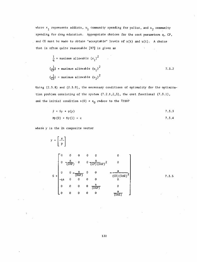
where x1 represents addicts, u
1 community spending for police, and u
2 community
spending for drug education.
and CE must be made to obtain
Appropriate choices for the cost parameters q, CP,
"acceptable" levels of x(t) and u(t). A choice
that is often quite reasonable [B7] is given as
1— = maximum allowable (x
1)2
= maximum
maximum
allowable (u1 )2
allowable (u2)2
Using (2.3.8) and (2.3.9), the
tion problem consisting of the
and the initial condition x(0)
= SY gY)
My(0) + Ny(1) = c
7.3.2
necessary conditions of optimality for the optimiza-
system (7.2.1,2,3), the cost functional (7.3.1),
= xo reduce to the TPBVP
where y is the 2n composite vector
S =
x
0 0 0
a° (DAP) 0
0 0 0
a 0(CP)(DAP)
2 0
0 0-a0(DAP)
-qa 0 0 0
0 0 0 0(DAP)
0 0 0 0 0
0
0
a
131
a
(CE)(DAE)2O.
0
a7:5ATT -
7.3.3
7.3.4
7.3.5
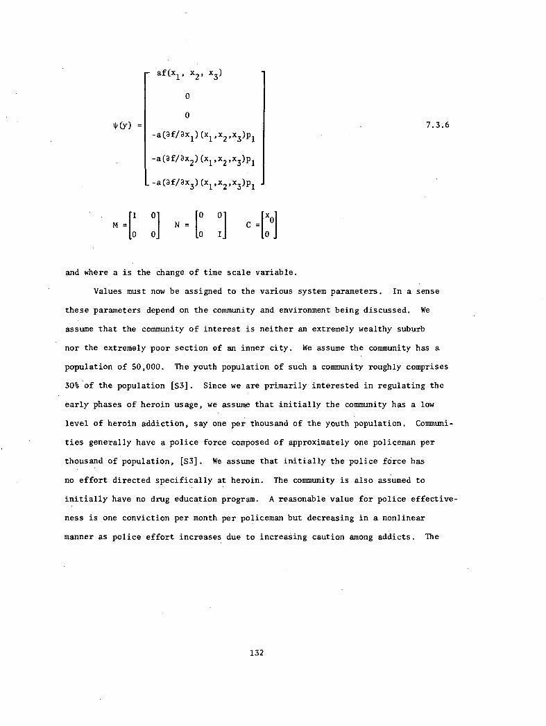
11)(y) =
— af(xl, x2, x3)
0
0
-a(3f/2x1)(xl,x2,x3)pl
-a(af/3x2)(xl,x2,x3)pl
_-a(3f/3x3)(xl,x2,x3)pl
I 01 M =
0 0.1N
0.1 Ixo]C =
0 I
7.3.6
and where a is the change of time scale variable.
Values must now be assigned to the various system parameters. In a sense
these parameters depend on the community and environment being discussed. We
assume that the community of interest is neither an extremely wealthy suburb
nor the extremely poor section of an inner city. We assume the community has a
population of 50,000. The youth population of such a community roughly comprises
30% of the population [S3]. Since we are primarily interested in regulating the
early phases of heroin usage, we assume that initially the community has a low
level of heroin addiction, say one per thousand of the youth population. Communi-
ties generally have a police force composed of approximately one policeman per
thousand of population, [S3]. We assume that initially the police force has
no effort directed specifically at heroin. The community is also assumed to
initially have no drug education program. A reasonable value for police effective-
ness is one conviction per month per policeman but decreasing in a nonlinear
manner as police effort increases due to increasing caution among addicts. The
132
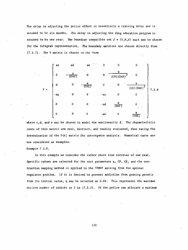
The delay in adjusting the police effort is essentially a training delay and is
assumed to be six months. The delay in adjusting the drug education program is
assumed to. be one year.. The- boundary compatible set J = {.V,M,N} must now be -chos.en
for the integral representation. . The...boundary matrices are .chosen directly from
(7.3.7). The V matrix is chosen in the form
V=
ac ad ae 0 0 0
a0
(I)A13
-act
0
0
0
0
a-TITAET
a0
(CP) (DAP) 2 0
.0 0 a
(CE)(DAE)2
-ac 0 0
- ada
(DAP)
-ae 0
0
a(DAE)
7.3.8
where c,d, and e may be chosen to model the nonlinearity f. The characteristic
roots of this matrix are real, distinct, and readily evaluated, thus easing the
determination of the - P(t) matrix for convergence analysis. Numerical cases are
now considered as examples.
Example 7.3.9.
In this example we consider the rather short time interval of one year.
Specific values are selected for the cost parameters q, CP, CE, and the con-
traction mapping method is applied to the TPBVP arising from the optimal
regulator problem. If it is desired to prevent addiction from growing greatly
from its initial value, q may be selected as 0.04. This represents the maximum
desired number of addicts as 5 in (7.3.2). If the police can allocate a maximum
133
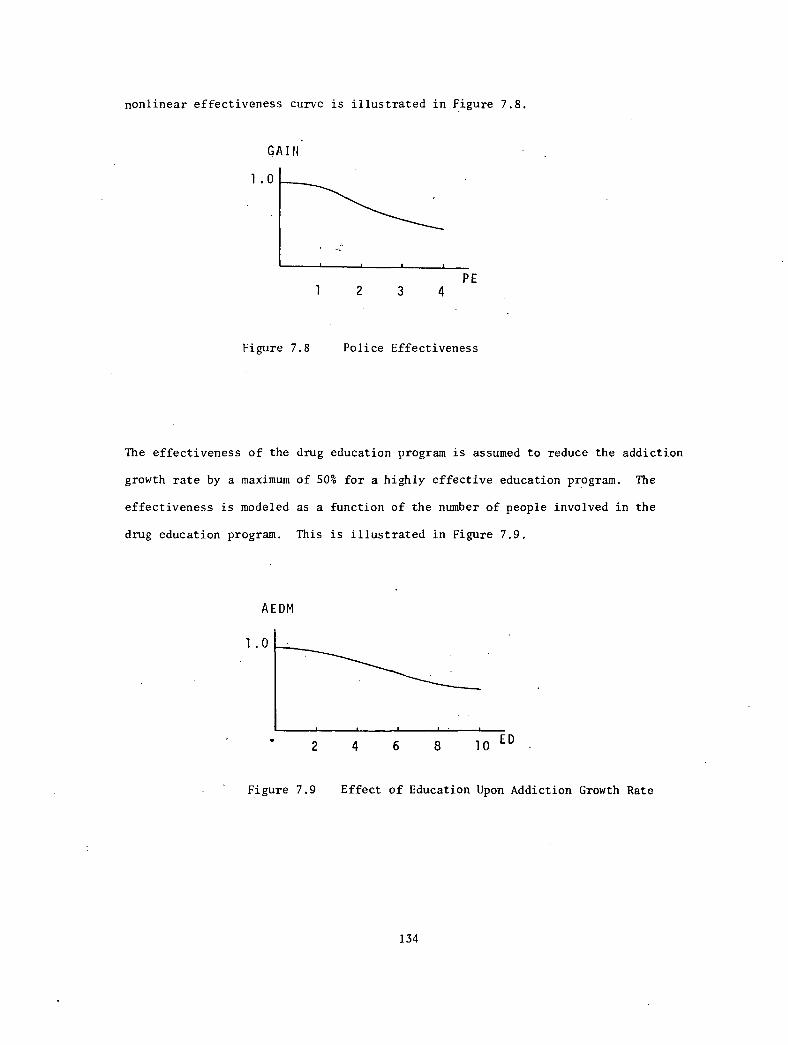
nonlinear effectiveness curve is illustrated in Figure 7.8.
GAIN.
1.0
PE1 2 3 4
Figure 7.8 Police Effectiveness
The effectiveness of the drug education program is assumed to reduce the addiction
growth rate by a maximum of 50% for a highly effective education program. The
effectiveness is modeled as a function of the number of people involved in the
drug education program. This is illustrated in Figure 7.9.
AEDM
1.0
•2 4 6 8 10
ED
Figure 7.9 Effect of Education Upon Addiction Growth Rate
134
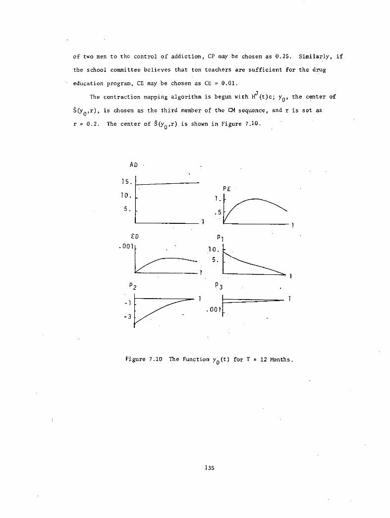
of two men to the control of addiction, CP may be chosen as 0.25. Similarly, if
the school committee believes that ten teachers are sufficient for the drug
education program, CE may be chosen as CE = 0.01.
The contraction mapping algorithm is begun with ie(t)c; y0, the center of
.(yo,r), is chosen as the third member of the CM sequence, and r is set as
r = 0.2. The center of g(yo,r) is shown in Figure 7.10.
AD
15
10.
5.
ED
. 001
1
PE
p2 p3
001
1
1
Figure 7.10 The Function y0(t) for T = 12 Months.
135
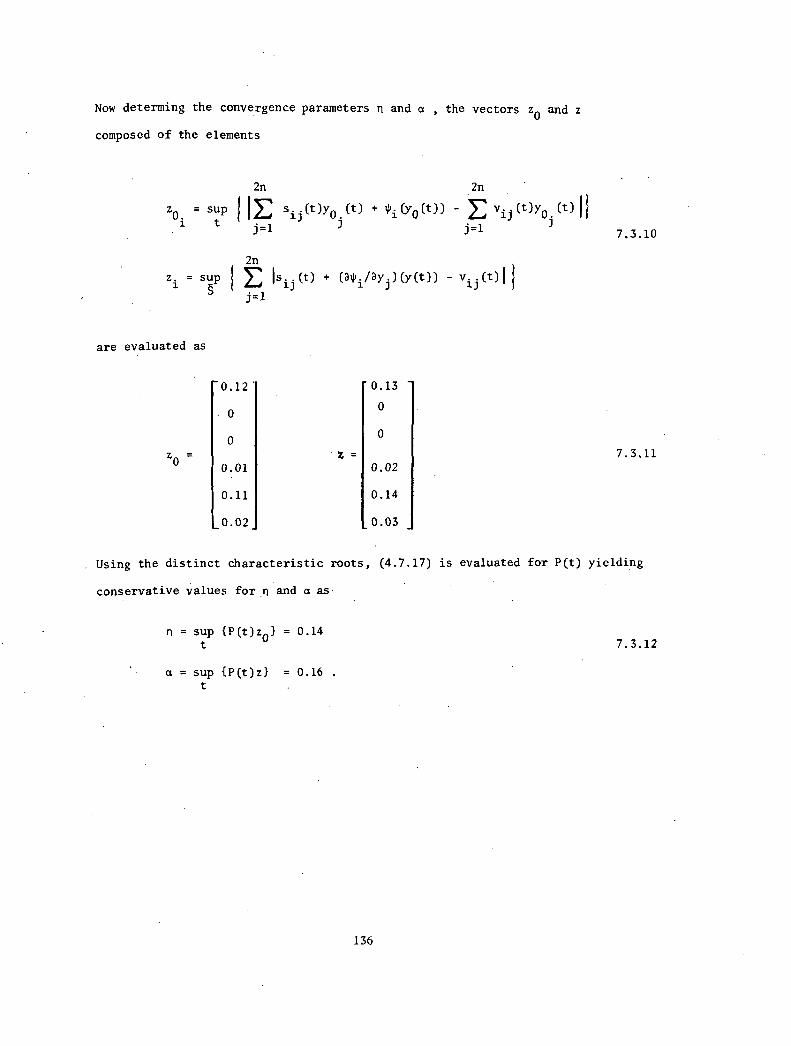
Now determing the convergence parameters n and a , the vectors z0 and z
composed of the elements
2n
zO.
= sup 1 1:E: sij(t)y0 (t) + *i(y0(t)) - I: vij (t)y0 (t) 11
1 t J Jj=1 j=1 7.3.10
2n
z. = sup :E: Is.-3.3 (t) 4. j(/aY)(Y(t)) - v..(01
j=1
are evaluated as
-0.12
0
0
0.13 -
0
0
z0 =
0.01"Z =
0.027.3.11
0.11 0.14
0.02 0.03
Using the distinct characteristic roots, (4.7.17) is evaluated for P(t) yielding
conservative values for n and a as.
n = sup (1)(t)z0} = 0.14t 7.3.12
a = sup {P(t)z} = 0.16 .t
136
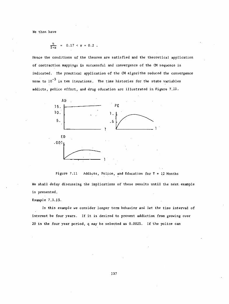
We then have
= 0.17 < r = 0.2 .1-a
Hence the conditions of the theorem are satisfied and the theoretical application
of contraction mappings is successful and convergence of the CM sequence is
indicated. The practical application of the CM algorithm reduced the convergence
norm to 10-3
in ten iterations. The time histories for the state variables
addicts, police effort, and drug education are illustrated in Figure 7.11.
AD
15.
10.
5.
ED
1
Figure 7.11 Addicts, Police, and Education for T = 12 Months
We shall delay discussing the implications of these results until the next example
is presented.
Example 7.3.13.
In this example we consider longer term behavior and let the time interval of
interest be four years. If it is desired to prevent addiction from growing over
20 in the four year period, q may be selected as 0.0025. If the police can
137
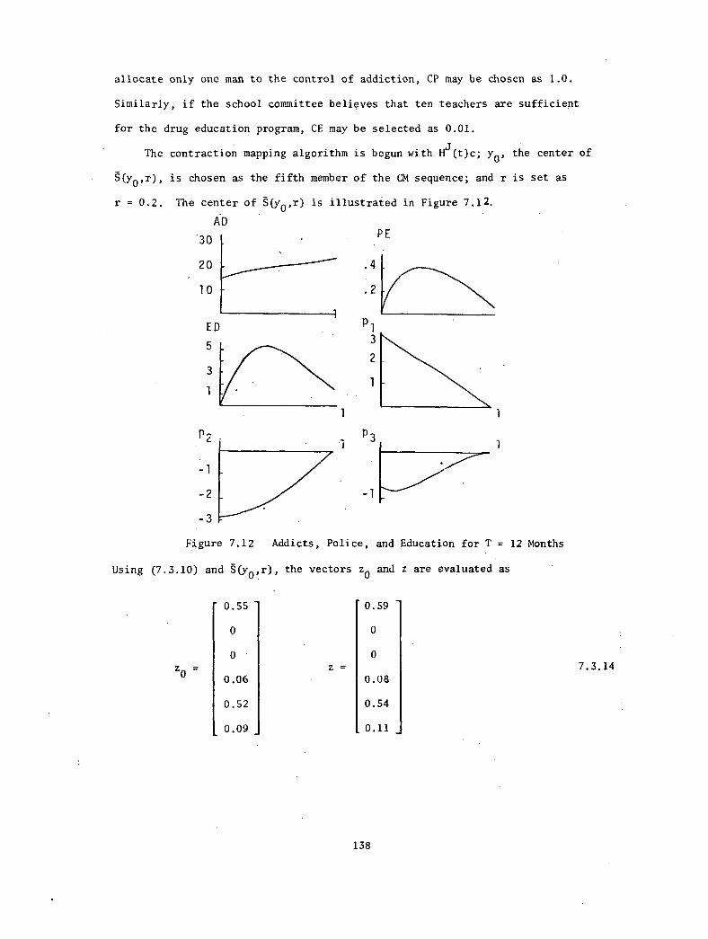
allocate only one man to the control of addiction, CP may be chosen as 1.0.
Similarly, if the school committee believes that ten teachers are sufficient
for the drug education program, CE may be selected as 0.01.
The contraction mapping algorithm is begun with Hj(t)c; yo, the center of
8(Y0,r), is chosen as the fifth member of the CM sequence; and r is set as
r = 0.2. The center of (yo,r) is illustrated in Figure 7.12.
AD
30
20
1 0
P2
-2
-3
Figure 7.12 Addicts, Police, and Education for T = 12 Months
Using (7.3.10) and 8(y0,r), the vectors z0 and z are evaluated as
1
. 2
3
2
p3
PE
•
0.55 - 0.59 -
0 0
0 0z =0 0.06
z =0.08
7.3.14
0.52 0.54
0.09 _ 0.11
138
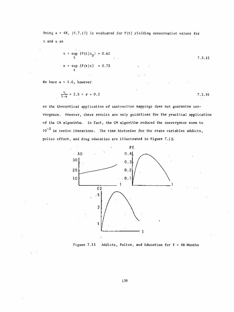
Using a = 48, (4.7.17) is evaluated for P(t) yielding conservative values for
n and a as
n = sup {P(t)z0} = 0.62t 7.3.15
a = sup AP(t)z} = 0.73t
We have a < 1.0, however
1-a = 2.5 > r = 0.2 7.3.16
so the theoretical application of contraction mappings does not guarantee con-
vergence. However, these results are only guidelines for the practical application
of the CM algorithm. In fact, the CM algorithm reduced the convergence norm to
10-3
in twelve iterations. The time histories for•the state variables addicts,
police effort, and drug education are illustrated in Figure 7.13.
PE.
AD 0.4
300.3
20 0.2
10 0 . 1
1
1
Figure 7.13 Addicts, Police, and Education for T = 48 Months
139
Discussion of Results
Although the stated purpose of this chapter is illustrative in nature,
perhaps one or two broad qualitative implicatons may be drawn from the results
of the two sample cases. First, the need for prompt action is clearly indicated.
With addiction growing at an exponential rate, any delay in dealing with the
problem is critical. In both examples, the police effort with a short reaction
time is used to begin removing the addiction core as quickly as possible. In
the first example, it is seen that the controller responds to the short term
situation with basically only a police effort. This is primarily due to the
fact that the controller does not have the time to establish a viable drug
education program. The second example is a longer term situation and the control
response is seen to be reasonably balanced, i.e., the optimal regulator responds
with both police effort and an education program. Again the police effort is
the first to be utilized, but the education program is brought into play as
quickly as possible and tends to deter long term growth. The drawing of
quantitative conclusions from these examples would be of dubious value. However,
the chapter illustrates that system modeling and optimal control theory may be
jointly utilized to obtain information and insight into policy formulation for
complex systems. Moreover, the chapter demonstrates that contraction mappings
is a useful concept and tool for both the theoretical and practical investigation
of nonlinear system control.
140
CHAPTER 8
SUMMARY, CONTRIBUTIONS AND RECOMMENDATIONS
8.1. Summary
In the broadest sense, the objective of this dissertation was t6 study the
theoretical and applied aspects of contraction mappings for the solution of
nonlinear control problems. This objective was achieved by considering the
theoretical and practical application of contraction mappings to the particular
issues of optimal regulation and controllability of nonlinear dynamical systems. .
It was shown in the study that application of the Pontryagin principle to
the optimal regulator problem yielded necessary conditions for optimality in
the form of a two point boundary value problem. Optimal system regulation Was
considered for. both. unconstrained and bounded controls and results were derived
for the. optimal regulation of linear dynamical systems and several classes of
nonlinear systems. By an..appropriate selection of boundary conditions, itWas
shown that the issue of controllability for dynamical Systems may also be reduced
to the study of two point boundary value problems.
The representation of two pointtoundary value problems'by an in'tegral
equation was then introduced and made it possible to consider.the solution of
two point'boundary value problems as the solution of corresponding operator
equations. The joint application of the integral representation and the implicit
function theorem provided new insight into the controllability of nonlinear
systems; The methods of contraction mappings and modified contraction. mappings
were then presented for the solution of operator equations. Convergence theorems
141
were presented for both methods, and translated convergence theorems were derived
for those operators arising from the optimal regulation of nonlinear systems.
A detailed investigation of the calculation of the theoretical convergence criteria
was conducted. Upper bounds were presented for the Lipschitz norm and derivative
norm, and various techniques for evaluating these bounds were introduced. In
particular, the use of simply structured matrices and similarity transformations
were considered. The use of partitioned matrices in these developments provide
considerable insight into the generic structure of the Green's matrices contained
within the integral representation.
Several numerical examples were presented to illustrate the theoretical and
practical application of contraction mappings to the regulation and control of
nonlinear systems. In particular, an example involving the regulation of
Van der Pol's equation was used to illustrate the calculation of the convergence
parameters and to demonstrate the manner in which the modified contraction mappings
method may be used to extend the range of applicability of contraction mappings.
An example considering the null controllability of the pitch motion of a satellite
with bounded control thrust was then presented. This example illustrated the
application of contraction mappings to an operator which did not satisfy differ-
entiability conditions. The Lipschitz norm rather than the derivative norm was
then used for the theoretical convergence analysis and to prove null controllabil-
ity from the initial point. The final example involved the development of a
dynamic model attempting to represent the causal, feedback structure of community
drug usage. Optimal regulator theory and contraction mappings were then used
to gain insight into how a community might best respond to a rapidly growing
heroin addiction problem. The various examples demonstrate that contraction
mappings is a useful tool for both the theoretical and practical investigation
of nonlinear system control.
142
8.2. Contributions
The author considers the following items to constitute the original contribu-
tions of this dissertation.
1. The determination of Green's functions in explicit form using simply
structured matrices and similarity transformations.
2. The development of insight into the generic structure of broad classes
of Green's functions by the use of partitioned matrices.
3. The development of a controllability theory for nonlinear dynamical
systems based on an integral representation of TPBVP's, the implicit function
theorem, and contraction mappings.
4. The theoretical and practical application of contraction mappings to a
nonlinear control problem with bounded input control and the subsequent use of the
Lipschitz norm to prove convergence for the nondifferentiable operator equation.
5. The theoretical and practical application of contraction mappings to the
optimal regulation of a dynamic model of a socio-economic system.
In addition, convergence theorems are presented for operators arising from
the optimal regulation of several classes of nonlinear systems. However, these
results are translations of the general theorems presented in Falb [F1] and in
that sense are not completely original.
8.3. Recommendations
In this section some areas of possible future research will be briefly
outlined. As indicated in the summary, the main thrust of this dissertation has
been directed toward the application of contraction mappings. However, Falb and
de Jong [F1] have succinctly revealed the close relationship which exists between
contraction mappings, modified contraction mappings, and Newton's method. The
143
first area for possible additional research lies in exploiting this relationship
and applying Newton's method to those operators arising from the optimal regula-
tion of nonlinear systems. Investigation of the convergence criteria for Newton's
method should yield additional insight into the theory of state regulation for
nonlinear systems. The second area of research lies in the extension of the
controllability results of Chapter 5. These results for the controllability of
nonlinear systems are essentially local in nature, i.e., they consider controll-
ability near the origin. However with additional analysis using the integral
representation, it should be possible to identify classes of problems for which
global results may be proved. The third and final area of recommended research
involves an in-depth analysis into the relationship between the drug system
model and the results of optimization. In particular, the data base for the
model, parameter identification, and a sensitivity analysis deserve significant
attention. In this manner, critical issues of the problem may be identified for
additional social investigation and data collection.
144
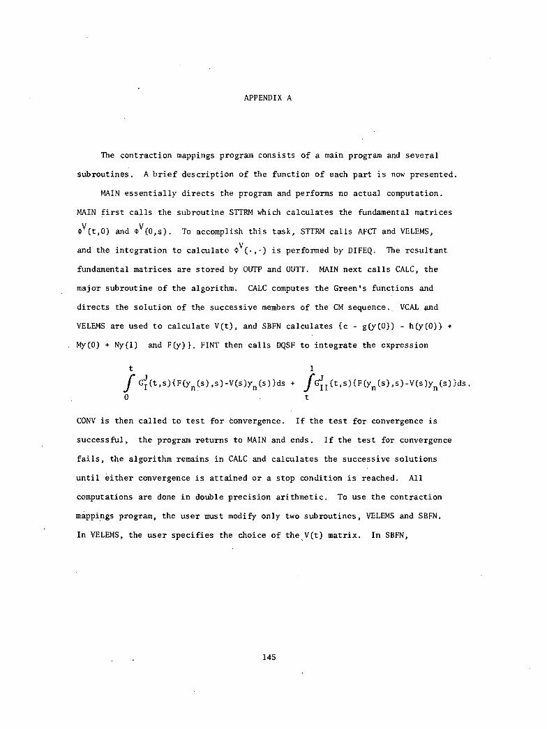
APPENDIX A
The contraction mappings program consists of a main program and several
subroutines. A brief description of the function of each part is now presented.
MAIN essentially directs the program and performs no actual computation.
MAIN first calls the subroutine STTRM which calculates the fundamental matrices
(DV(t,0) and clY(0,$). To accomplish this task, STTRM calls AFCT and VELEMS,
and the integration to calculate OV(.,.) is performed by DIFEQ. The resultant
fundamental matrices are stored by OUTP and OUTT. MAIN next calls CALC, the
major subroutine of the algorithm. CALC computes the Green's functions and
directs the solution of the successive members of the CM sequence. VCAL and
VELEMS are used to calculate V(t), and SBFN calculates {c - g(y(0)) - h(y(0)) +
My(0) + Ny(1) and F(y)1. FINT then calls DQSF to integrate the expression
1
jr G(t,$){F(y n(s),$)-V(s)yn(s))ds + )(G
II(t,$){F(yn(s),$)-V(s)yn(s)}ds.I
0
CONV is then called to test for convergence. If the test for convergence is
successful, the program returns to MAIN and ends. If the test for convergence
fails, the algorithm remains in CALC and calculates the successive solutions
until either convergence is attained or a stop condition is reached. All
computations are done in double precision arithmetic. To use the contraction
mappings program, the user must modify only two subroutines, VELEMS and SBFN.
In VELEMS, the user specifies the choice of the V(t) matrix. In SBFN,
145

the user specifies the differential equation y = F(y,t) and the boundary
condition g(y(0)) + h(y(1)) = c. The program contains many comment statements
to ease application.
146
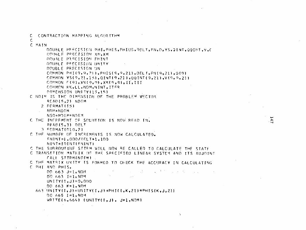
C CONTRACTION MAPPING ALCORITHMCC MATN
ncluBLE PPECISTON PHI,PHISIPHIUS,DELT,EN.D 9 YS.)INT,QQINT,V,C ITUHLE PPECTsInm XN,XMnour1LE wk=c1sION FNINTDOUBLE PRECISION UNITYnouBLE PRECISTON UNummoN PHI(9.9,;'1),PHIS(C.P.21),DEIT,EN(q,21),D(9)COMMON YS(9,21.15),OTNT(9,21),UOINT(9,21),Vlq,P,2])COr'!mON r(9),xN(9,q),xm(q,q),II,IIIcommm RK,LL.NDM,NINT,ITFRDTmENSION UNITY(15,15)
C NDIm IS THE DIMENSION OF THE PROBLEM VECTORREAD(5,2) NDTM
2 FORMAT(T5)NOM=NDTMNSO=NDIM*NDIM
C THE INCREMENT OF SOLOTTON IS Nrvi READ IN.RFA0(5,3) DELT
3 EORMAT(610.2)C THF NUMBEP OF INCREMENTS IS NOW CALCULATED.
FNINT=1.0DO/DFLT+1.100NINT=IDINT(ENINT)
C THE SURROUTINE srl-Pm WILL NOW RE CALLED TO CALCULATE THF STATF.C TRANSITION MATRIX OF THE SPECIFIED LINEAR SYSTEM AND ITS ADJOINT
CALI. STTPM(NOTM)C THF MATRIX UNITY IS FORMED TO UiECK THE ACCURACY IN CALCULATINGC PHI AND PHIS.
DO 663 J=1,NOM60 663 I=1,NDMUNITYIT,J)=0.090DO 663 K=1,NOM
66 IINITY(I,J1=UNITY(I,J14-PHI(I,K,21)*PHTS(K,J,21)DO 665 1=1,ND4WRITE(6,664) (UNITY(T,J), J=1,NDM)
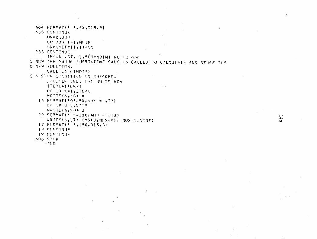
664 FORMAT(' ',5)(,015.91665 CONTINUE
ON=0.0D000 333 I=I,NOIMUN=UNITY(I,i1+ON
313 CONTINUEIF(UN .GT. 1.500*NOIM) GO TO 606
C NOW THF MAJOR SUPROUTINE CALC IS CALLED TO CALCULATE AND STORE THF:C NFW SOLUTTUN.
CALL CALC(NDIM1(7 4 sTrIP CONDITNN IS CHECKED.
IF(ITER .E.O. 151 '10 TO 606ITER1=ITER+1no 19 K=1,ITER1WRITF(6,16) KFORMAT('01,5X,4HK = 03)On 19. J=1,ND1MWRTTE(6,?01 J
?0 cORMAT(' 1 ,10X,411,1 = ,I3)WR ITE(6,17) (YS(J,NOS,K1, NDS=1,NINT1
17 FORMAT(",15X,015.811P CONTTNUFlq CONTINUE
606 sTnpFN0
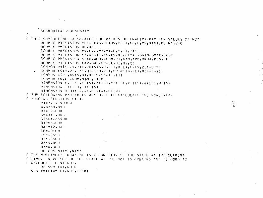
SUBROUTINE .SBENINDIMI
C THIS SuRPouTINE CALC)LATES THE VALUES OF FN=FIYI-Vg01, EPP. VALUES nF NDTnnuBLF. PHI,PHIS,PHIOS,OELT,EN,O,YS,QINT,DOINT,V,CDOULE PRECISION XN,XM001191. PRECISIIIN YV,F,7,YI,YT,G,H,TT,TTTDOUILE PRECISION X10(?,X30/i.X5,X6,7FIXT,GAIN,GmAX,DGDPOfluFALC PRECTSTUN GTAU,A0DIAEDNI,PI,AAm,AVB,9RPA,PCS.FFDOUBLE RRECISTIU EAP,Q4E,CP,CE,01,02,,,13COmmON PHI(9'.9.?1),PHIS(9.q,21)iDELT,ENI9,21),0(91COMMoN YSI9,21,151,0INT(9,21),D'ANT(9,7.11,V(9,9,21)commoN c.(9)0(N(9,9)0o1(9,q),TI,IttcnmwIN KK,I.L.N0m,NINT,ITFPDIMENSION YV(151,E(15).ZIT5).1,1(15).YTI15),GI15),H(I5)DIMENSION TTI15),TTT(15)DIMENSION OFDxT(4,4),PCS(41.FE(9)
C THE FOLLOWING VARIABLES ARE USEU, TO CALCULATE THE NONLINEARC EoRCING FUNCTION FIT).
(1 1=3.1415930)AvB=.0000T=I2.000GMAx=1.000GTAU=.255D0040-6.0D0OAE=I2.000CE=.01D0C9-.25rm01-.94on02=0.0D003=0.000O0 600NOT=I,NINT
C THF NONLINEAR EQUATION IS A FuNCTION OF THE.' STATF AT THU CuPRENTC TIME. A VECTOR np THF STATE AT THE NOT IS CREATED ANC IS usFn TOC CALCULATE F AT NOT.
00.599 I=I,Nolm599 YVIII=YSII,NDT,ITFRI
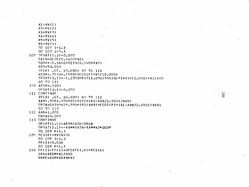
X1=YV(1)X2=YV(2)X3=YV(3)X4=YV(4)X5=YV(5)X6=YV(61DO 10? 1=1,3DO 102 J=2,3
10? 9F0XT(1,J)=0.000GAIN=DCOS(0.3600*X2)DGDP=-0.3600*DSIN(0.1600*X21AOD=50.0001F(X3 .GT. 10.000) GO TO 110AE0M=.75D0+.2500*DCOS(PI*v3/10.0001DFOXT(3,1)=-(.2500AtPI/10.000)*DSIN(PI*X3/10.000)*X1/A00Gn TO 111
1.10 AFOM=.5000OF0XT(3,11=0.000
111 CONT1NUFIF(X1 .GT. 60.000) GO TO 112AAM=.5D0+.500v0SIN(P1*(X1-AVB/2.0001/AVB)DROA=GAIN*X2*.500*(PI/AVB)*CCOS(PI*(X1-AVB/2.0D0)/AVB)GO TO 113
112 AAM=1.0P0DRDA=0.000
113 CONTINUFDFDXT(1,1)=AEDM/A0D-DROADFDXT(2,11=-AAM*GAIN-AAM*X2*DGDPDO 109 K=1 13
109 PCS(K)=YV(K+3)do 10R 1=1,3FF(1)=0.000DO 108 K=1,3
108 FF(T)=FF(1)+0FOXT(1,K)*PCS(K)GRA=AEDM*X1/A00RRPE=AAM*GAIN*X2
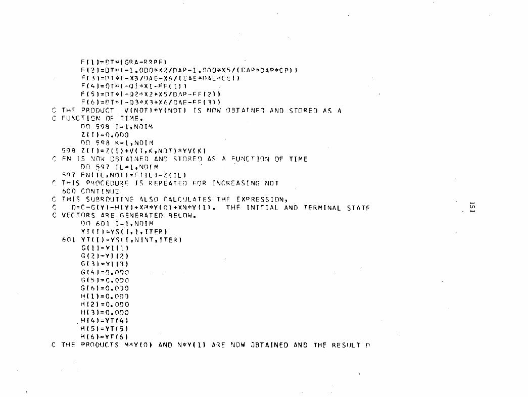
F(1)=DT*(GRA-PRPF)F(2)=DT*(-1.000*X:?/DAP-1.000*X51(CAP*DAP*CP))E(3)=PT*(-X3/DAE-X6/(CAE*DAE*CE))F(4)=QT*(-01*Xl-FF(1))F(5)=OT*(-1)2*X24-X5/DAP-FF(2))F(6)=DT*(-Q3*X3+X6/0AF-FF(1))
C THF PRODUCT N(NOT)*Y(NDT) TS NOW OBTATNE1 ANO STORED AS AC FUNCTION OF TIME.
no 598 I=1.NDIM7(1)=0.000on 598 K=1,NDIM
599 Z(I)=7.(1)+V(I,K,NOT)*YV(K)C FN IS NOW OBTAINED AND sTrIRED AS A FUNCTION OF TIME
00 597 IL=1,NDIMg47 FWIL,NOT)=F(IL)-7.(IL)
r THIS PROCEDuE IS REPEATED FOR INCREASING NOT600 CONTINUE
C THIS SUBROUTINE ALSO CALCULATES THE EXPRESSION,C 0=C-G(Y)-H(Y)+XM*Y(0)+XN*Y(1). THF INITIAL AND TERMINAL STATFC VECTORS ARE GENERATED BELOW.
on 601 I=1,NOIMYI(I)=YS(I,1,ITER)
601 YT(I)=YS(I,NINT,ITER)G(1)=YI(1)G(2)=YI(2)G(3)=YT(3)G(4)=0.090G(5)=C.000G(6)=0.0D0H(1)=0.00014(2)=0.090H(3)=0.090H(4)=YT(4)H(5)=YT(5)H(6)YT(6)
C THF PRODUCTS M*Y(0) AND N*Y(1) ARE NOW OBTAINED AND THE RESULT fl
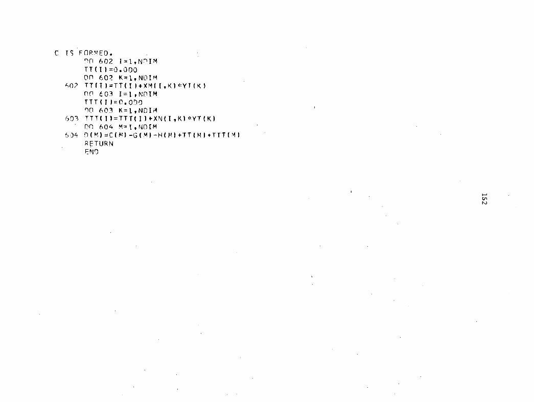
C. TS FORmE0.7)11 602 1=1,NnIMTT ( I 1=0.00000 602 K=1.NDIMTTTT )=TT( )+XM( I,K)tYT(Knr 603 1=1,NrypiTTT( T )=0.0!•)0On 603 K=1,NDIA
603 TTT( 1)=TTT( I )*XN( ,K)*NeT (K)NI 604 M=I,NCIiM
604 D(M)=C( m) -G(M)-H(M)+TT(M )+TTT(1RFTURNENO
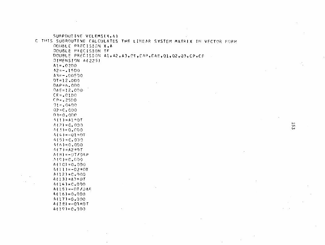
SUBROUTINE VELEMSIX,A1C THIS SUBROUTINE CALCULATES THE LINEAR SYSTEM MATRIX IN VECTOR FORM
DOUBLE PRECISION X,ADOUBLE PRECISION TFDOUBLE PRECISION A1,42,A3,PT,CAP CAE Q1,02,03,CP,CEDIMENSION A(z25)
A2=—.15DOA17—.00500OT=12.000DAP=6.000o4E=12.0no.CF=.0100CP.25D0:)17.04000?=C.000o3-o.onoA(1)=Al*nrA(?)-o.opoA(3)=0.000
A(5).C.000'W-170.000A(7)=A2*OTA(81=-1)T/DAP..'1()=C.000A(10)=0.000A(II)=-02*OTA(12)=0.000A(13)=A3*OT4(14)=C.000A(15)=-1')T/DAE4(16)=0.000A(171=0.000A(1R)=-034cDTA(191=0.000
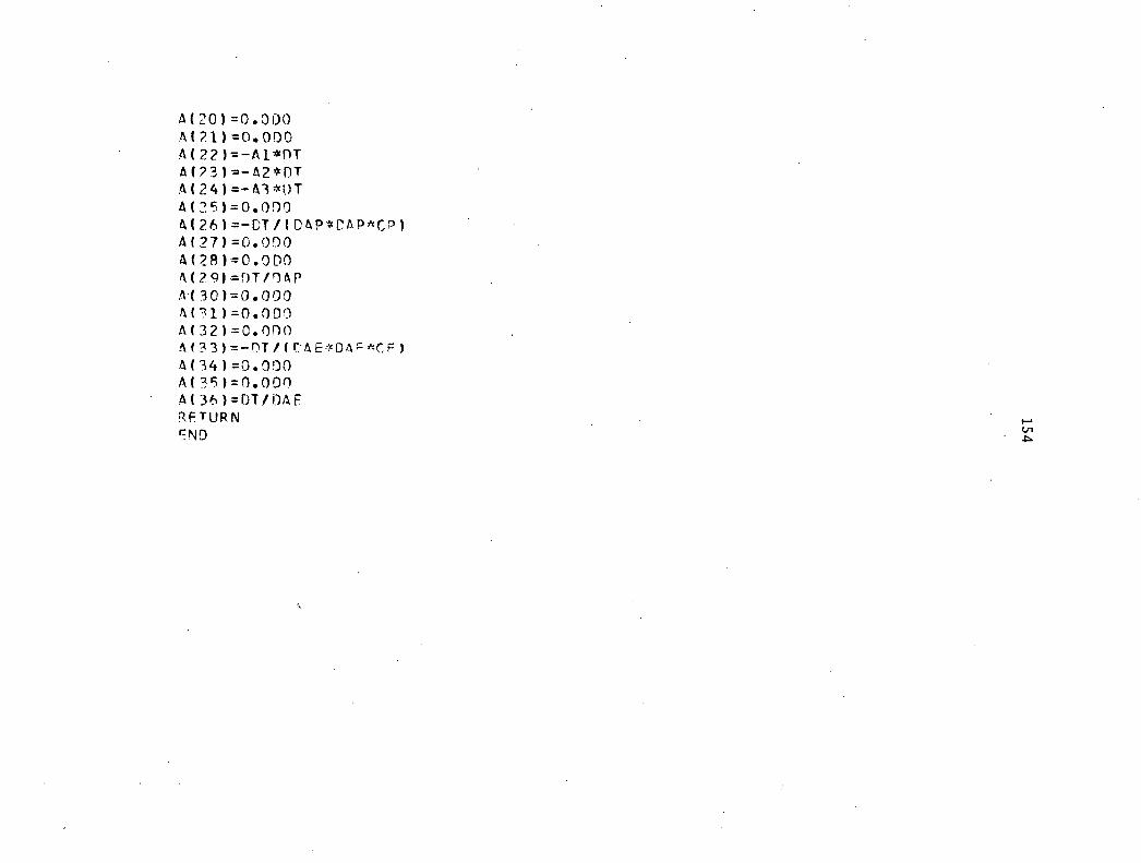
A(20)=0.000A(21)=0.000A(22)=—A1*DTA(23)=—A2*0TA(24)=—A3exOTA(25)=0.000A(26)=-0T/(0AP*CAP*CP)A(27)=0.000A(28)=0.000A(29)=0T/OAPA130)=0.000A(71)=0.000A(32)=0.000A(33)=—DT/(CAE,x0AF*CE)A(34)=0.000A(35)=0.000A(36)=DT/OAFRETURNEND
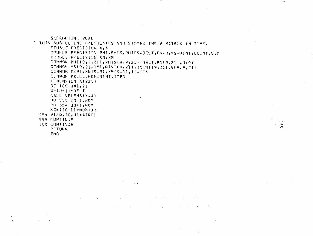
SURROUTINE VCALc THiS SUBROUTINE CALCIJLATFS AND STORES THE V MATRIX IN TIME.
nOuBLE PRECISION X,AOpUBLE PRECISION PHI,PHTS,PHIOS,DELT,FN,D,YS,AINT,CAINT,V,CDOUBLE PRECISION XN,XMCDMMON PHI(9,9,21),PHIS(9,9,21),DELT,EN(9,21)T0(9)COMMON YS(9,21,15),OINT(9,21),DDINT(9,21),V(9,9,21)COMMON C(9),XN(90)0(m(9,q),II,IIT.COMMON KK,LL,NDm,N(NT,ITERDIMENSION A(225)DO 100 J=1,21)(=(.1-1)*DELTCALL VELEMS(X,A)00 555 1Q=1,NDMnn 554 J0=1,NDMKQ=( TO-1)*NDM+JOVIJO,I0,J)=4(K(J)
555 CONTINUF100 CONTINUE
RFTURNEND
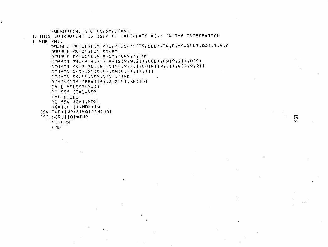
SUBROUTINE AECT(X,SM,DERVI
C THIS SUBROUTINE IS USED TO CALCULATE V(.) TN THE INTEUATION
C FOR PHI.DOUBLE PRECISION PHI,PHIS,PHIOSIDELT,EN,D,YS,:)INT,OQINT,V,CDOUBLE DRECTSION XN,xMDOUBLE PRECISION X,SM,DERV,A,TMP
crimmoN PHI(q0,21),PHIS(q19,21),DELT,EN(9,21),D(9)COMmoN YS(c1,21,15),QINT(9,21),QQINTI(1,21),W,19,211
COMMON C(9),XN(9,9),Xm(9,0),IT,TIT
COMMCN ICKILL,NOM,NINT,TTERnimF.NsION DERV(15),A(775),SM(15)
CAIL VELEMS(X,A)
DO 599 10=1,NOMTmP=0.0D0r)O 554 Ji)=1,NOMKO--(J0-1),rNDM+T(,)
554 Tmp.TmP+A(KOI*Sm(JO)fg5 DEPV(TO)=TmP
PETURNEND
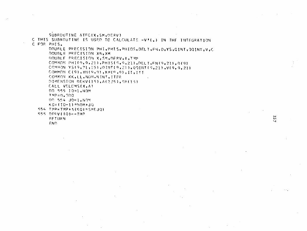
SUBROUTINE ATEC(X,SM.DERV)C THTS SUBROUTINE IS USED TO CALCULATE -V°(.1 IN THF INTEGRATIONC FOR PHIS.
nnuRLE PRECISION PHI,PHIS,PHIOS,DELT.FN.D,YS,QINT,MINT,V,CDOUBLE PRECISION XN,XMnnuBLE PRECISION X,SM,OFPV.A,T1PComMnN PHI(9.9.21),PHIS(c;,(1,211,DELT,FN(q,211,0(9)Crimm,:m YS(,?1,151.0INT(Q,21).Q9INT(q,21).V(9.9,21)(7.0MrAnN C(9),xmq,q),xm(0,9),IT,ITiCW9InN KK,LL,NDM.NTNT,TTERDIMENS1(3N DERV(15),A(225),SM(15)CALL VFLEMS(X,A)nn 955 I0=1,NDMTrop=0.200Dr 554 J0=1,Nnm
KO=IT(J-1)DM+J(J954 TMP.TMP+A(KO)SM(Jp)555 DERVITO1=-TrIP
RETURNENn
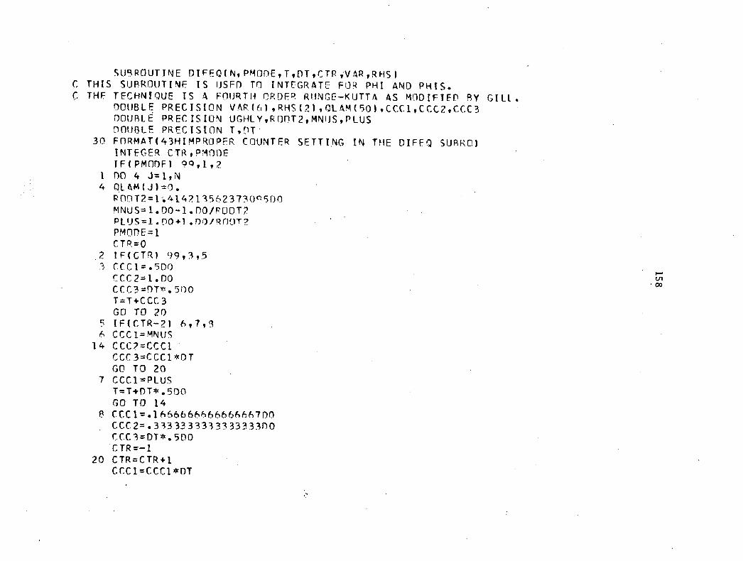
SUBROUTINE. DIFEON,PMODE,T,OTICTRiVAR,RHSIC THIS SUBROUTINE IS USED rn INTEGRATE FOR PHI AND PHIS.C THF TECHNIQUE IS A FOURTH ORDER RtINGE-KUTTA AS MODIFIED RY GILL.
DOUBLE PRECISION VARI61,RHSI2I,OLAM(50),CCC1,CCC2,CCC3DOUBLE PREC ISION UGHLY,ROOT2,MNUS,PLUSDOUBLE PRECISION TOT'
30 FORMAT(43HIMPROPER COUNTER SETTING IN THE DIFFQ SURROIINTEGER CTROMODEIFIPMODFI 99,1,2
1 nn 4 J=1,N4 DLAM(J)=0.
ROOT2=1..41421156237300500MNUS=1.00-1.00/POOT2PLUS=1.00+1.D0/RnoT2PMODE=1CTR=O
.2 IF(CTR) 99,3,53 CCCI=.5D0CCC2=1.D0CCC3=DT*.500T=T+CCC3GO TO 20
5 IF(CTR-2) 6,7,96 CCC1=MNUS14 CCO=CCC1
CCC3=CCC1*DTGO TO 20
7 CCC1=PLUST=T+DT*.500GO TO 14
P CCC1=.1666666666666667D0CCC2=.3133333333333333D0CCC3=DT*.500CTR=-1
20 CTR=CTR+1CCC1=CCCI*DT
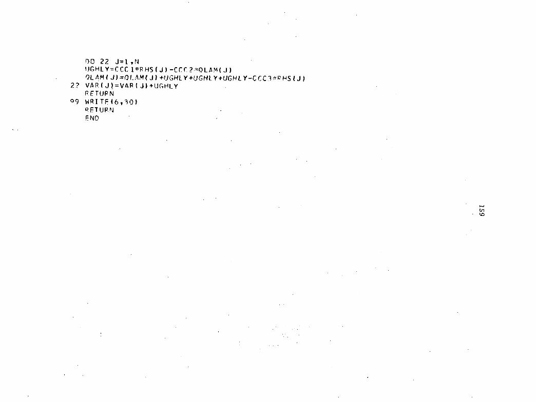
DO 22 J-.=1,NUGHLY=CCC1*RHS(JI-CCC2YtOLAM(J)OLAM(J)=OLAM(J)+UGHLY+UGHLY+UGHLY-CCC3*RHS(J)
22 VARW=VAR(J)+UGHLYRETURN
99 WRITE(6,30)PETURNFND
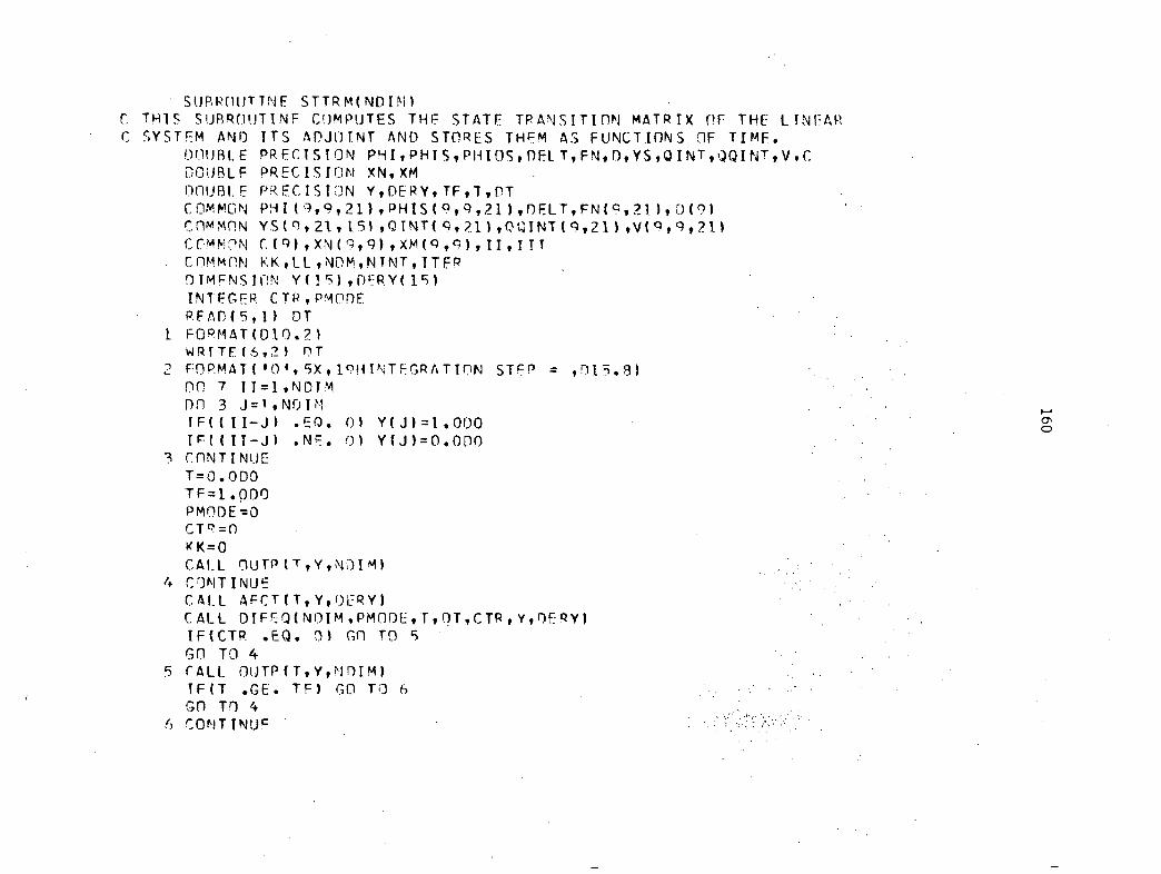
SUBROUTINE STTRM(NDIM)C 'THIS SUBROUTINE CoMPUTES THF STATE TRANSITION MATRIX OF THE LTNEARC SYSTFM AND TTS ADJOINT AND STORES THEM AS FUNCTIONS OF TIMF.
DOUBLE PRECTSTON PHI,PHIS,PHIOS,DELT,FN,D,YS,QINT,QQINT,V,CDOUBLE PRECISION XN,XMDOUBLE PRECISION Y,DERY,TF,T,OTCOMMON PHI(c4,9,211,PHISI9,q,211,0ELT,FNIC:,211,0(91COMMON YS(c1,21,151,0TNT(c0.11,0QINTI9,211,V(q,c),211COMMON CIR1,XN(9,91,XMCR,9),II,TITCOMMON KKILL,NOM,NTNT I TTFPDIMENSION Y(15),WTRY(151INTEGER CTR,PMO))EREAD(5,11 DT
1 FORMAT(010.21WRTTE(5,2) nT
2 FORMAT( 10 0,5X,I9HINTEGRATTON STEP = ,015.31no 7 II=1,NOTMon 3 J=1,NDIM
.E0. 0) Y(J)=1.000IFITII—J1 .NF. 01 11(.11=0.000
3 CONTINUET=0.000TF=1.000PMODE=0
KK=0CALL OuTP(T,Y,NDIM)
4 CANTINUECALL AECT(T,Y,DCRY)CALL DIFFATNDIM.PMODE,TOT,CTR,Y,DERY1IFICTR .EQ. 01 Gn TO 5GO TO 4
5 CALL OUTPIT,Y,NDIM)TETT .GE. TF) GO TO 6GO TO 4
6 CONTINUE
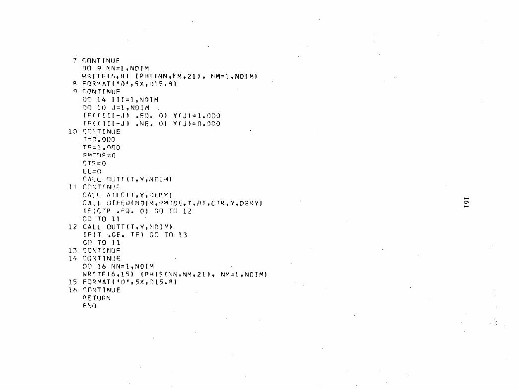
CONTINUEDO 9 NN=1.NOIMWRITE(604) (PHI(NN,rM,21), NM=1,NDIM)FORMAT('0',5X,015.3)
9 CONTINUEDo 14 III=1,NDTM00 lo J=1,NDIMIF((III-J) .EQ. 0) Y(J1=1.000IF((III-J) .NE. Y(J)=0.0r0
10 CONTINUET=0.0D0Tc=1.0D0PMODE,--0CTR=0LL=0CALL OUTT(T,Y,NDIM)
11 CONTINUECALL ATECAT,Y,IEPY)CALL DIFEO(NDIM,PMOOE,T,DT.CTR,Y,DERY)IF(CTP .EQ. 0) GO TO 12GO TO 11
1 2 CALL OUTT(T,Y,NF)IM)IF(T TF) GO TO 13GO TO 11
13 CONTINUE14 CONTINUE
DO 16 NN=1,NOIMWRTTE(6,15) (PHIS(NN.NM.211, NW=1,NCIM)
1.5 FORMAT('0 1,5X.015.9)16 CONTINUE
PETURNENO
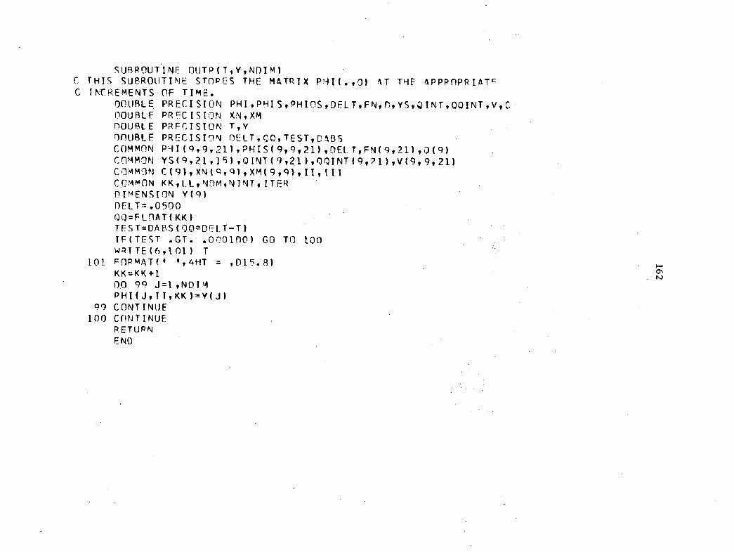
SUBROUTINE OUTP(T,Y,NDIM)C THIS SUBROUTINE STOPES THE MATRIX PHI(.0) AT THE APPPnPRIATFC INCREMENTS OF TIME.
DOUBLE, PRECISION PHI,PHISOHIOS,DELT,FNI D,YS.QINT,00INT.V,C .DOUBLE PRFCISION XN,XMnouBLE PRFCISION T,YwuBLE PRECISION DELT,CO,TEST,OA5SCOMMnN PAI(9.9,21),PHIS(9,9,21),DELT,FN(9,21)0(9)COMMON YS(9,21,15),QINT(9921)00INT(901),V(9,9,21)COMMON C(9),XN(99 910N(90),II,IIICOMMON KK,LL.NDM,NINT,ITERDIMENSION Y(9)DELT=.050000=FLOAT(KK)TEST=DAP,S(Q0*DFLT-T)IF(TEST .GT. .000100) GO TO 100WRITE(6,101) T
101 FORMAT(",4HT = 0015.8)KK=KK+1DO 99 J=1.NDIMPHI(J,TIOCK)=Y(J)
99 CONTINUE100 CONTINUE
RETURNFNO
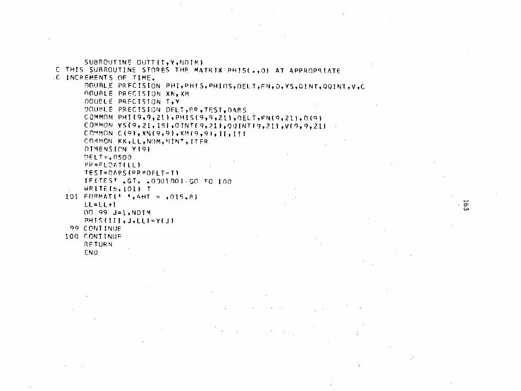
SUBROUTINE OUTT(T,Y,NDIM)C THIS SUBROUTINE STORES THF MATRIX PHISt.,0) AT APPROPRIATE.0 INCREMENTS OF TIME.
nntiBLE PRFCISION PHI,PHIS,RHIOS,DELT,EN,D,YS,QINT,OQINT,V,CDOUBLE PRECISION XN,XMDOUBLE PRECISION T,YOnoelE PRECISION DELT,RR,TEST,DARSCOMMnN PHI(9,9,21),PHIS(919,21),DELT,FN(9,211,D(91COMMON YS(9,21,151,0INT(9,211,0MINT(9,211,V(9,9,21)cn.imrIN c(9)oN(9,9),xm(9,9),TI,ITTcrimmoN KK,LL,Nom,NINT,TTERDIMENSInN Y(9)DELT=.05D0RR=FLOAT(LL)TEST=DAPS(RR*DELT-T1IF(TEST .GT. .000100), GO TO 100WRITE(6,101) T
101 FORMAT(' ',4HT = ,015,p)
LL=LL+100 99 J=1,NDIMPHIS(III,J,LL)=Y(J)
99 CONTINUE100 CONTINUF
RETURNENO
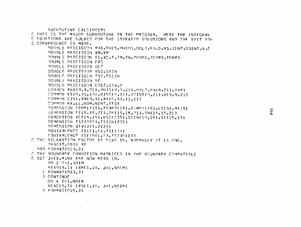
SUP:ROUTINE CALEANDIm)C THIS IS THE MAJOR SUBROUTINE TN THE PROGRAM. HERE THE INTFGRALC EDUATIONS ARE SOLVED FOR THE ITERATED SOLUTIONS AND THF TFST EnqC CONVERGENCE IS MADE.
nCMBLE PRECISInl PMPHIS,PHIOS,DELT,EM,D,YSDOUBLE PRECISION XN,XMImpltE PRECISION SI,XC,T,TM,TN,TEmPI,TEMP2,TEMP3TluBLE PRECISION FPSDOUBLE PRECISION DETDOUBLE PRECISION VSI,SIINonoBLP_ PRECISIN TSI,TSIINDOUBLE PRF.CISION REDOUBLE PRECISION COST,CIV,7commcIN PHI(9,9,21),PHIS(9,q,21),DELT,EN(R,211,D(9)COMMON YS(0,?1,15),OINT(c,21),QCINT(9,21),v(9,9,21)commr)NcommoN KKILL,NDM,NINT,ITERDIMENSION TEMP1(15),TEMP2(15),P2MP'.(15),L(15),M(15);)IMENSION T(15,15,21),TM(15,15,.71),TN(15,15,211DIMENSION XC(15,19),VSI(P25),SIIN(1 63,15),SI(15,15)DtmENSICN TSI(??5),TSIIN(2?.51DImENSION AIV(211,l(21)FOUIVAIENCE (SI(1,1),TSI(1))E00IVALENCF ISITN(1,1),TSIINMY
C THILT RELAXATION FACTOR IS READ IN. NORmALLY TT IS ONE.REAC(,555) RF
55 FORMAT(D10.2)C THE 40uNDARY CONDITION MATRICES TN THF BOUNDARY COMPATIBLEC SET J-1..(V,M,N) ARF Nnw READ IN.
nn 2 I=1,NDImREAD(5.11 (XM(I,J), J=1,NOIM)
I FORMAT(010.2)2 CONTINUEDO 4 I=I,NDIMREAD(5,3) (XN(I,J), J=1,NOIM)
3 Fop:MATO:110.21
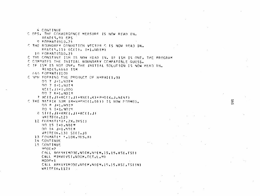
4 CONTINUEr FPS, THE CONVERGENCE MEASURE IS NOW READ IN.
RFAO(5,q) EPS? PMAT(010.21
C THE BOUNDARY CoNOITTON VECTOR C TS NOW READ IN.RFAfl(5,10) (C11), I=1,NnTm)
10 FORMAT(D10.,1C THE CONSTANT ISM TS Nnw READ IN. IF ISM IS nNE, THE PROGRAMC CoMPUTFS THE INITIAL BOUNDARY COMPATIBLE GUESS.C. IF ISM IS NOT ONF, THE INITIAL SOLUTION- IS NOW READ TN.
READ(5,666) JSM(s6'3 FORMAT(I10)
C NOW FOPMING TUE PRODUCT OF N*PHI(1,0)Do 7 J=1,NOTMno 7 I=1,NDIMXC(I,J)=0.000DO 7 K=1,NDIM
7 XC(I,J)=XC(1,J)4-XN(I,K)=PHI(K,J,NINT)C THE MATRIX SUM (m+N*PH1(1,0)1) I s Now FoRMED.
DO P J=1,NDIMDO B I=1,NOP1
8 SI(I,J)=XM(I,J14-XC(I,J)WRITE(6,121
12 FORMAT('0',2X,2HSI)no 15 I=1,NDImOn it J=1,NOIMWRITE(6,131 SI( I,J)
13 FORMAT(' ',10X,015.8)14 CONTINUE15 CONTINUE
WIDE=?CALL ApRAy(MODE,NoTm,N0IM,15,15,VSI,TS11CALL mINV(VSI,NDIM,OET,L,M)MODF=1CALL ARRAY(MODE,NDIN,NOIM,15,15,VSI,TSIIN)WRITE(6,1121
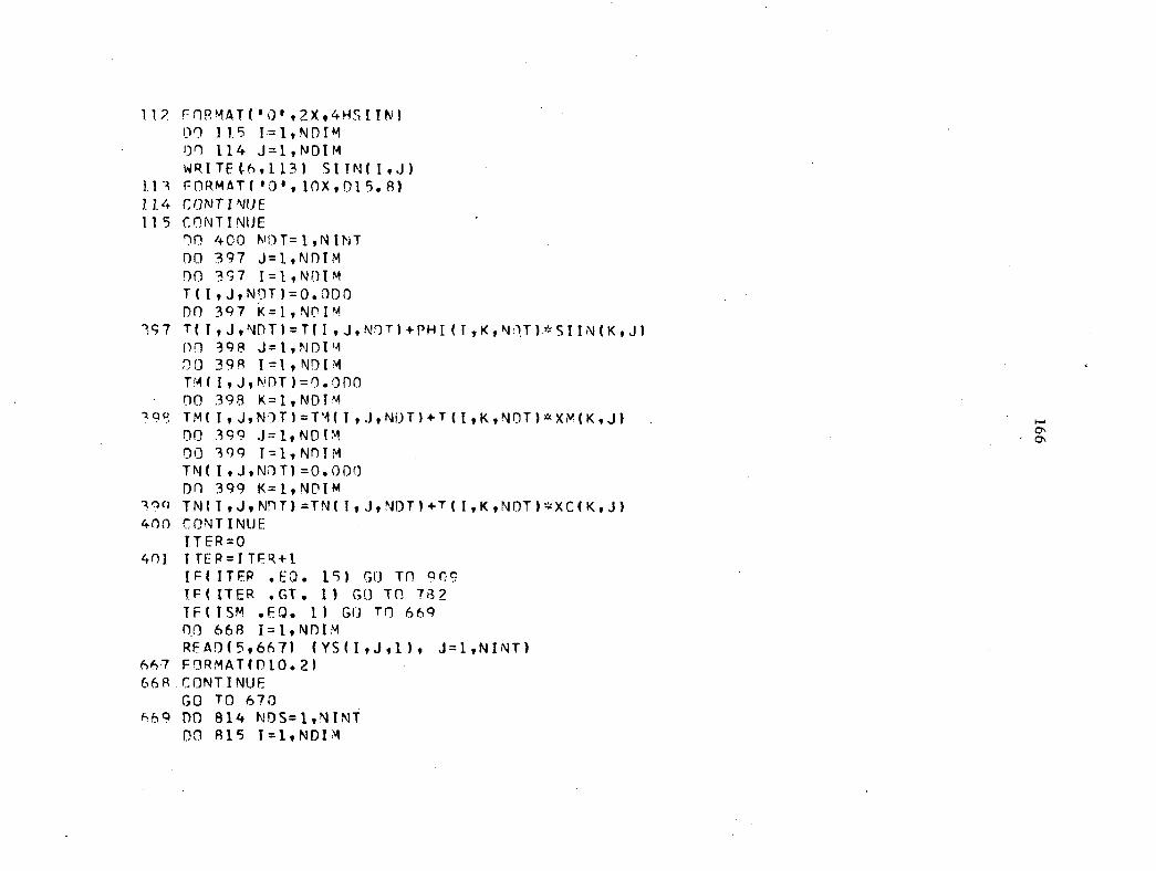
112 FOPMAT('0°,2X,4HSITN)09 115 I=1,NDIMDO 114 J=1,NDIMWRITE(6,1131 SIIN( I,J)
111 FORMAT( 101,10X,015.81 .114 CONTINUE115 CONTINUE
no 400 NDT=1,NINTDO 397 J=1,NDIMDO 397 I=1,NDIMT(I,J,NOT1=0.0D0DO 397 K=1,NOINI
197 T(I,J,NDT)=TII,J,NOT1+PHI(T,K,NO.T).*SIIN(K,j1no 398 J=1,NDImDO 398 I=IonimTM(I,J,NoT)=0.000DO 398 K=1,NDIM
199 TMII,J,NIT1=T1(T,J,NOT1+T(I,K,NOT14XM(K,J)DO 399 J=1,NDIM • (3\DO 399 I=1,NDIMTN(I,J,NDT1=-0.0D0Do 399 K=1,NOIM
199 TN(I,J,NDT)=TN(I,J,NDT1+T(I,K,NOT)*XC(K,J1400 CONTINUE
ITER=0401 ITER=ITER+1
IFfITER .E0. 15) GO Tfl 9C(7IF( ITER .GT. 11 GO TO 782IF(ISM .FQ. 11 GO To 669RO 668 I=IontmREAD(5,6671 (YS(I,J,1), J=1,NINT1
667 FORMAT(D10.2166R CONTINUE
GO TO 670669 DO 814 NDS=1,NINT
no 815 I=1,NDIM
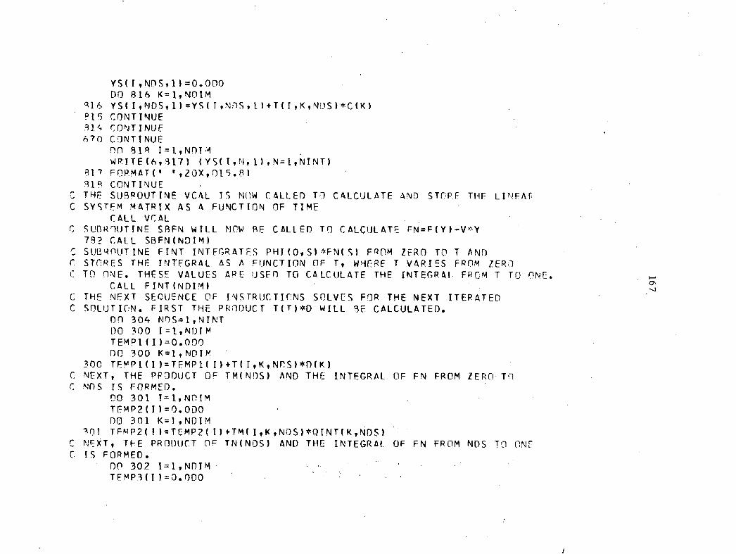
YS(I,NDS,1)=0.000DO 816 K=1,NDIM
916 YS(I,NDS,1)=YS(I,NDS,1)+T(I,K,NOS)*C(K)915 CONTINUE114 CONTINUE670 CONTINUE
DO 818 I=1,NDIMWRITE(691171 (YS(I0,1),N=1,NINT)
817 FORMAT(",20X,015.91919 CONTINUE
.„ THE SUBROUTINE VCAL IS NOW CALLED TO CALCULATE AND STORE THF LINFAPC SYSTEM MATRUX AS A FUNCTION OF TIME
CALL VCALC SUBROUTINE SBFN WILL NOW BE CALLED TO CALCULATE FN=F(Y)-V,%Y
792 CAI..L SBEN(NDIM)SUBROUTINE FINT INTFGRATFS PHI(0,S)*FN(S) FROM ZERO TO T AND
C STORES THF INTEGRAL AS A FUNCTION OF T, WHERE T VARIES FRom ZEROC TO ONE. THESE VALUES APE USED TO CALCULATE THE INTEGRAI. FRCM T TO ONE.
CALL FINT(NDIM) cr,
C THE NEXT SEQUENCE OF INSTRUCTIONS sno/Es FOR THE NEXT ITERATEDC SOLUTION. FIRST THE PRODUCT T(T)*D WILL BE CALCULATED.
00 304 NDS=1,NINTDO 300 I=1,N1)IMTEMP1(I)=0.0D0DO 300 K=1,NDIM
300 TEMPI(I)=TFMR1(I)+T(I,K,NDS)*D(K)C NEXT, THE PRODUCT OF TM(NDS) AND THE INTEGRAL C1F FN FROM zERo. TOC mns IS FORMED.
DO 301 T=1,NptmTEMP2(I)=0.opono 301 K=1,NDIM
101 TEMP2())=TEMP2(I)+TM(I,K,NDS)*QINT(K,NDS)C NEXT, TFE PRODUCT OF TN(NDS) AND THE INTEGRAI. OF FN FROM NDS TO ONFC IS FORMED.
DO 302 I=1,NntmTEMP3(i)=0.0D0
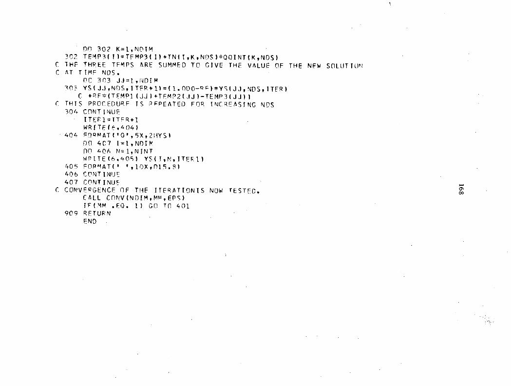
no 302 K=1,NOIM302 TEMP3(I)=TEMP3(I)+TN(I,K,NOS)*Q0INT(KODS)
C THF THREE TFMPS ARF SUMMED TO GIVE THE VALUE OF THE NFW S(ILUTIONC AT TIMF NDS.
PO 303 JJ=1,NDIM303 YS(JJ,NDS,ITER+1)=(1.000-RF)*YS(JJ,NDS,ITER)
C. 4-RE*(TEMP1(JJ)+TEMP2(JJ)-TEMP3(JJ))C THTS PROCEDURE TS REPEATED FOR INCREASING NOS304 CONTINUE
ITER1=TTER+1
WRITE(6,4(?4)404 FO0MAT('0',5X,211YS)
DO 4C7 1=1,NOIMno 406 N=1,NiNTwPITE(6,405) YS(I,N,ITEP1)
405 FORMAT(' ,,lox,n15.8)406 CONTINUE407 CONTINUE-
C CONVFRGENCE OF THE ITERATIONIS NOW TESTED rp. 00CALL CONV(NDIM,MM,EPS)IE(MM .FQ. I) GO TO 401
909 RETURNEND
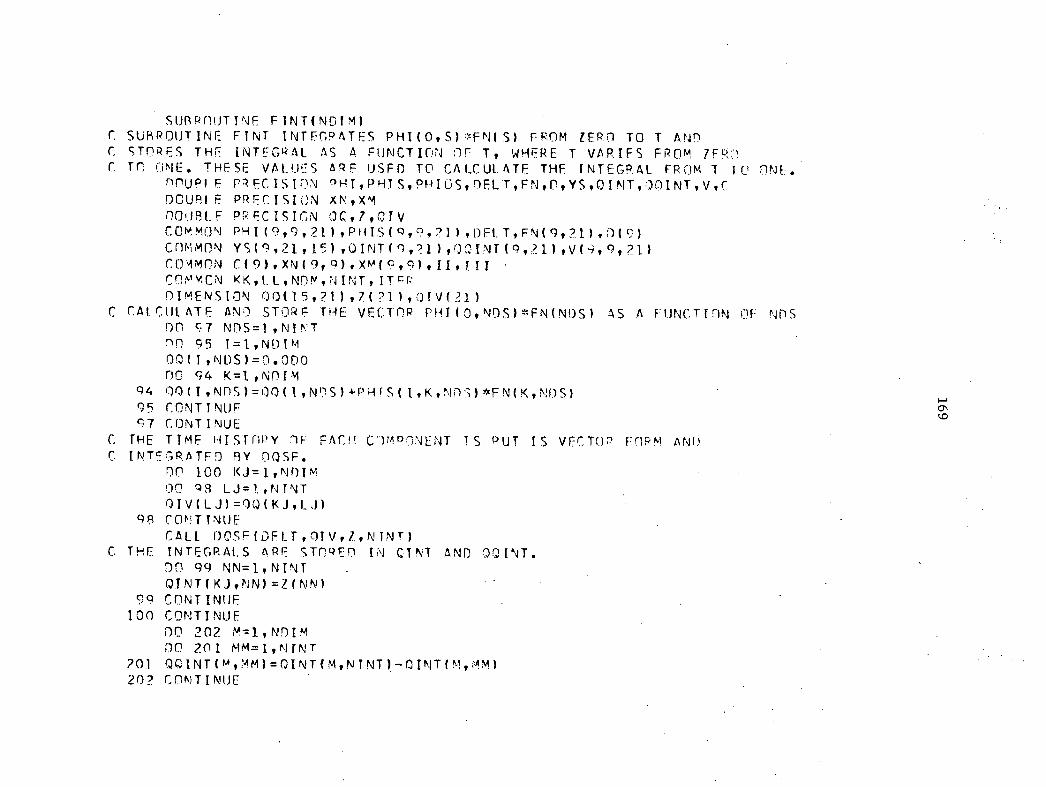
SUBROUTINE FINT(ND(M)r SUBROUTINE FTNT INTEGRATES PHI(0,S)*EN(S) FROM ZERO TO T ANDC STORES THE INTEGRAL AS A FUNCTIflN OF T, WHERE T VARIES FROM lFflC rn ONE. THESE VALUF.S ARP USED TO CALCULATE THE INTEGRAL FROM 1 To ONE.
0OURIF PRECISION BHI,PHTS,PHIOS,DFLT,EN,O,YS,OINT,WINT,V,CDOUBIE PRECISION XN,XMDOUBLE PRECISION OC,7,CIVCOMMON RHI(e,e,21),PHIS(9,9,?]),DELT,EN(9,21),0(e)crimmoN YS(9,21,15),OINT(9,?1),OINT(9,21),V(9,9,21)crAmnN c(9),xN(9,9),v0(9,9),I1,11rcrPmcN KK,LL,NOM,NINT,ITFPDIMENSION 00(15,?1),7(?1),CIV(211
C CAICULATE AND STORE THE VECTOR PHI(0,NDS)*EN(N0S) AS A FUNCTION OF NDS00 97 NDS=1,NINT2n 95 I=1,NDIM0Q(1,NDS)=0.000no e4 K=1,NDIM
94 00(I,NDS)=00(1,NDS)4PHfS(I,K,NDS)*EN(K,NOS)95 CONTINUE97 CONTINUE
C THE T TMF HIsrnPy 2F EACH COMDONENT TS, PUT I S VECTOR FORM ANDC INTE'GRATFD BY 00SE.
or 100 K.J=1,NOIM00 93 LJ=1,NINT01V(LJ)=QQ(KJ,LJ)
9R CONTINUECALL DOSF(DELT,OIVIZ,NINT)
C THE INTEGRALS ARF srnizEn IN CINT AND OQINT.DO 99 NN=1,NINTQINT(KJ,NN)=Z(NN)
99 CONTINUE100 CONTINUE
DO 202 M=1,NOIM00 201 MM=1,NINT
POI QQINT(m,MM)=OINT(M,NINT)-OINT(M,MM)202 CONTINUE

Page intentionally left blank
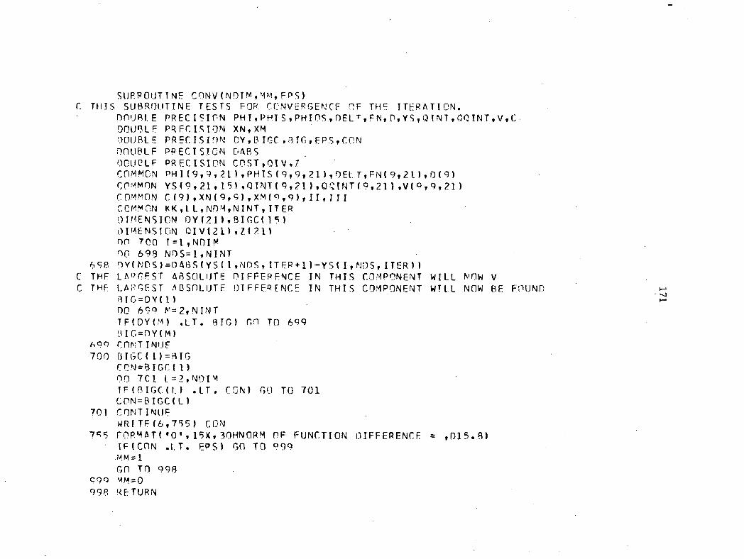
SUBROUTINE CONV(NDTM,Mm,FPS)C THIS SUBROUTINE TESTS FOR CONVERGENCE nF THE ITERATION.
nnUBIE PRECISION PHI,PHIS,RHIOS,DELT,FN,O,YS,0TNT,00INT,v,C.DOUBLE PRECISION XN,XMDOUBLE PRECISION CY,BIGC.BIG,'Eps,CoNDOUBLE PRECISION DABSDOUBLE PRECISION CnST,0Iv,7COMMON pHI(9,9,21 1 ,PHIS(9,9,21),DELT,FNI9,2II,O(9)COMMON YS(9,21,1),OINT(9,21),Of;INT(9,21),VIP,9,21)COMmON C(9),XN(9,9),Xm(9,9),II,IIICOMMON 10<0.1,NDM,NINT,ITERDIMENSION DY(211,BIGC(15)DIMENSION OIV(21),1.I211nn 700 I=1,NnIMDO 699 NnS=1,NINT
698 DY(NOS)=DABSIYS(I,NDS,ITER+1)-YSII,NDS,ITER))C THF LARGEST ABSOLUTE DIFFERENCE IN THIS COMPONENT WILL Nnw Vc THE,. LARGEST ABSOLuTE DIFFERENCE IN THIS COMPONENT WILL NOw BE FOUND
ITG=DYII)00 699 P=2,NINTTF(DY(m) .LT. BIG) Gn To 699BIC=DY(M)
61qc? CnNTINUF70o BIGC(1)=BIG
CrN=BIGCt1)DO 7C1 1=2,NDImIEIBIGC(L) .LT. CCN) GO TO 701CON=BIGCILI
701 CONTINUEWRITE(6,755) CON
7q5 FORmATI,01,15X,3OHNORM OF FUNCTION DIFFERENCE ,D15.8)IF(cnN .LT. EPS) GO TO 999A.m=1on TO 998
999 mm=0
99R RETURN

Page intentionally left blank
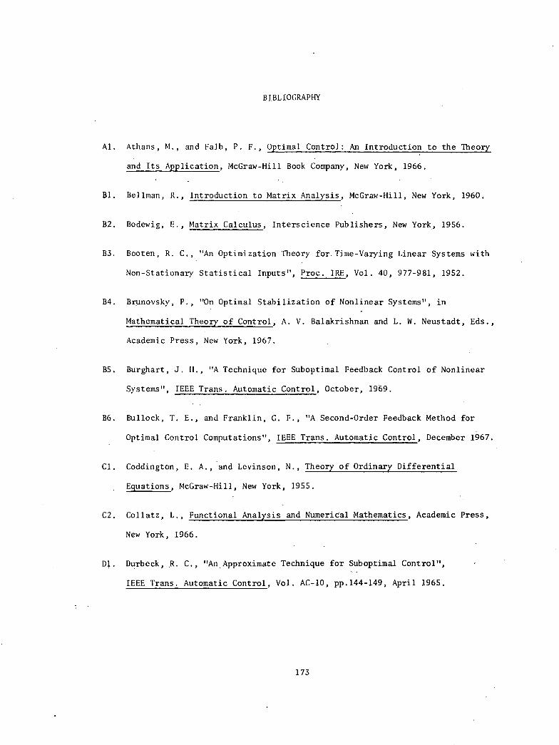
BIBLIOGRAPHY
A1. Athans, M., and Falb, P. F., Optimal Control: An Introduction to the Theory
and Its Application, McGraw-Hill Book Company, New York, 1966.
B1. Bellman, R., Introduction to Matrix Analysis, McGraw-Hill, New York, 1960.
B2. Bodewig, E., Matrix Calculus, Interscience Publishers, New York, 1956.
B3. Booten, R. C., "An Optimization Theory for.Time-Varying Linear Systems with
Non-Stationary Statistical Inputs", Proc. IRE, Vol. 40, 977-981, 1952.
B4. Brunovsky, P., "On Optimal Stabilization of Nonlinear Systems", in
Mathematical Theory of Control, A. V. Balakrishnan and L. W. Neustadt, Eds.,
Academic Press, New York, 1967.
B5. Burghart, J. H., "A Technique for Suboptimal Feedback Control of Nonlinear
Systems", IEEE Trans. Automatic Control, October, 1969.
B6. Bullock, T. E., and Franklin, G. F., "A Second-Order Feedback Method for
Optimal Control Computations", IEEE Trans. Automatic Control, December 1967.
C1. Coddington, E. A., and Levinson, N., Theory of Ordinary Differential
Equations, McGraw-Hill, New York, 1955.
C2. Collatz, L., Functional Analysis and Numerical Mathematics, Academic Press,
New York, 1966.
Dl. Durbeck, R. C., "An Approximate Technique for Subop.timal Control",
IEEE Trans. Automatic Control, Vol. AC-10, pp.144-149, April 1965.
173
D2. Dyer, Peter, and S. R. McReynolds, The Computation and Theory of Optimal
Control, New York, Academic Press, 1970.
F1. Falb, P. L., and deJong, J. L., Some Successive Approximation Methods in
Control and Oscillation Theory, Academic Press, New York, 1969.
F2. Ferrar, W. L., Finite Matrices, Oxford University Press, London, 1951.
F3. Forrester, J. W., Industrial Dynamics, M.I.T. Press, M.I.T., Cambridge,
Mass., 1961.
F4. Forrester, J. W., Principles of Systems, Wright-Allen Press, Cambridge,
Mass., 1968.
F5. Forrester, J. W., Urban Dynamics, M.I.T. Press, M.I.T., Cambridge, Mass.,
1969.
F6. Forrester, J. W., World Dynamics, Wright-Allen Press, Cambridge, Mass.,
1971.
F7. Forrester, J. W., "Industrial Dynamics: A Major Breakthrough for Decision
Makers", Harvard Business Review, July-August 1958.
F8. Friedland, B., "A Technique of Quasi-Optimal Control", J. Basic Engrg,
Vol. 88, June 1966.
G1. Gantmacher, F. R., The Theory of Matrices, New York, Chelsea Publishing
Company, 1959.
G2. Garrard, W. L., et.al., "An Approach to Suboptimal Feedback Control of
Nonlinear Systems", Internatl. J. Control, Vol. 5, pp.425-435, November 1967.
174
G3. Gershwin, S. B., and Jacobson, D. H., "A Controllability Theory for
Nonlinear Systems", IEEE Trans. Automatic Control, Vol. AC-16, No. 1,
February 1971.
H1. Holtzman, J. M., Nonlinear System Theory, Prentice Hall, Englewood Cliffs,
New Jersey, 1970.
J1. Jazwinski, A. H., "Quadratic and Higher-Order Feedback Gains for Control
of Nonlinear Systems", AIAA J., Vol 3, pp.925-935, May 1965.
K1. Kalman, R. E., "Contributions to the Theory of Optimal Control",
Bol. Soc. Mat. Mexico, pp.102-119, 1960.
K2. Kalman, R. E., "When Is a Linear System Optimal?", J. Basic Engineering,
(ASME Trans.), Vol. 86, pp. 1-10, 1964.
K3. Kalman, R. E., Bo,.and Narenda, "Controllability of Linear Dynamical Systems",
Contributions to Differential Equations, Vol. 1, 1962.
K4. Kantorovich, L. V., and Akilov, G. P.; Functional Analysis.in Normed Spaces,
Macmillan, New York, 1964.
K5. Kleinman, D. L., On the Linear Regulator Problem and the Matrix Riccati
Equation, Electronic Systems Laboratory Report ESL-R-271, M.I.T., tambridge,
1966.
L1. Lee, B.L., and Markus, L., Foundations of Optimal Control Theory, John Wiley
and Sons, Inc., New York, 1967.
L2. Long, R.S., "Newton-Raphson Operator.; Problems.with Undetermined Endpoints",
AIAA J., 3, pp. 1351-1352, 1965.
175
L3. Longmuir, A. G., and Bohn, E. V., "The Synthesis of Suboptimal Feedback
Control Laws", IEEE Trans. Automatic Control, Vol. AC-12, pp. 775-758,
December 1967.
L4. Lukes, D. L., "Optimal Regulation of Nonlinear Dynamical Systems";
SIAM J. Control, Vol. 7, No. 1, February 1969.
N1. Newton, Gould, and Kaiser, Analytical Design of Linear Feedback Controls,
John Wiley and Sons, Inc., New York, 1957.
01. Ogata, K., State Space Analysis of Control Systems, Prentice-Hall, Englewood
Cliffs, New Jersey, 1967.
P1. Pearson, J. D., "Approximate Methods in Optimal Control", J. Electron Control,
Vol. 13, pp.453-469, 1962.
P2. Picard, E., Traite d'Analyse, 3rd ed., Vol. III, Gauthiers-Villars, Paris,
1928.
P3. Pugh, A. L., DYNAMO User's Manual, M.I.T. Press, Cambridge, Mass., 1963.
R1. Rees, F. J., and Flugge-Lotz, I., Minimum Fuel Control of a Pitch Motion
of a Satellite in Circular Orbit, SUDAAR No. 352, Dept. of Aero. and Astro.,
Stanford Univ., Stanford, Cal., 1968.
R2. Roberts, E. B., The Dynamics of Research and Development, Harper and Row,
New York, 1964.
R3. Roberts, E. B., et. al., "Narcotics and the Community: A System Simulation",
To be published in the Journal of Health, May-June, 1972.
176
Sl. Simmons, G. F., Topology and Modern Analysis, McGraw-Hill, New York, 1963.
S2. Schoenberger, M., "Optimization and Implementation of System Control Laws",
Proc. 4th Ann. Allerton Conf. Circuit and System Theory, pp.557-566, 1966.
S3. Statistical Abstract of the United States: 1970, U. S. Bureau of the Census,
U. S. Department of Commerce.
T1. Turnbull, H. W., and Aitkin, A. C., An Introduction to the Theory of
Canonical Matrices, Blakies and Son, Ltd., London, 1932.
W1. Weiner, N., The Extrapolation, Interpolation and Smoothing of Stationary
Time Series, Technology Press, M.I.T., Cambridge, Mass., 1949.
W2. Willis, B. H., "The Frequency Domain Solution of Regulator Problems",
Presented at the 1965 JACC, Troy, N. Y., June 22-25, 1965.
Z1. Zadeh, L. A., and Ragazzini, J. R., "An Extension of Weiner's Theory of
Predictions", J. Appl. Phys., Vol. 21, pp.945-955, 1950.
177

Page Intentionally Left Blank
BIOGRAPHICAL NOTE
William Robert Killingsworth, Jr. was born in on
He attended public schools in Birmingham and graduated from
Banks High School in June, 1963. Mr. Killingsworth was awarded a Gorgas Science
Foundation Scholarship and entered Auburn University in June, 1963. He graduated
from Auburn in June, 1966, receiving the degree of Bachelor of Science in Aero-
space Engineering with highest honors. The President's Award for the School of
Engineering was awarded to Mr. Killingsworth, and he was elected to Phi Kappa Phi
and Tau Beta Pi honorary societies.
Mr. Killingsworth entered the Department of Aeronautics and Astronautics
at M.I.T. in September, 1966 and was elected to the Sigma Xi honorary society
the following year. He received the degree of Master of Science in June, 1968.
His S.M. thesis was entitled "Computation Frames for Strapdown Inertial Systems".
Through June, 1966 his graduate study was supported by a National Science Founda-
tion Graduate Fellowship. In September, 1968 Mr. Killingsworth became a research
assistant at the M.I.T. Measurement Systems Laboratory, where he pursued his
doctoral research.
During summers, Mr. Killingsworth has been employed by the Hayes International
Corporation (1966), working on a range safety analysis; the Electronic Systems
Laboratory, M.I.T. (1968), working on a computer display algorithm; and The
Analytic Sciences Corporation (1969), working on a navigation and control project.
Mr. Killingsworth is married to the former Joyce Caryn of Westwood,
Massachusetts.
179