Measurements of thermal properties of icy Mars regolith ...authors.library.caltech.edu/30059/1/Siegler2012p17729J_Geophys_Res... · Measurements of thermal properties of icy Mars

Measurements of thermal properties of icy Mars regolith analogs

Matthew Siegler,1,2 Oded Aharonson,2 Elizabeth Carey,2 Mathieu Choukroun,3

Troy Hudson,3 Norbert Schorghofer,4 and Steven Xu2,5

Received 18 August 2011; revised 20 December 2011; accepted 20 December 2011; published 7 March 2012.

[1] In a series of laboratory experiments, we measure thermal diffusivity, thermalconductivity, and heat capacity of icy regolith created by vapor deposition of water belowits triple point and in a low pressure atmosphere. We find that an ice-regolith mixtureprepared in this manner, which may be common on Mars, and potentially also present onthe Moon, Mercury, comets and other bodies, has a thermal conductivity that increasesapproximately linearly with ice content. This trend differs substantially from thermalproperty models based of preferential formation of ice at grain contacts previously appliedto both terrestrial and non-terrestrial subsurface ice. We describe the observedmicrophysical structure of ice responsible for these thermal properties, which displacesinterstitial gases, traps bubbles, exhibits anisotropic growth, and bridges non-neighboringgrains. We also consider the applicability of these measurements to subsurface ice onMars and other solar system bodies.

Citation: Siegler, M., O. Aharonson, E. Carey, M. Choukroun, T. Hudson, N. Schorghofer, and S. Xu (2012), Measurements ofthermal properties of icy Mars regolith analogs, J. Geophys. Res., 117, E03001, doi:10.1029/2011JE003938.

1. Introduction

[2] Thermal properties of icy regolith are an importantcomponent in modeling and measuring the migration andpresence of volatile-rich subsurfaces of rocky bodiesthroughout the Solar System. Thermal properties of icyregolith are also vital in quantifying surface and subsurfacevolatile content in remote sensing observations (namelyinfrared and microwave). Measurements of thermal proper-ties of terrestrial icy soils have been made [e.g., Kersten,1949; Lachenbruch et al., 1982], but ice formationmechanisms are generally unknown. Numerous models ofthermal properties of terrestrial icy soils have been devel-oped [e.g., Johansen, 1975; Farouki, 1981; Lachenbruchet al., 1982], but need to be extrapolated to extraterrestrialand extreme terrestrial conditions. Terrestrial icy soils typi-cally experience periods in which migration of water in theliquid phase occurs, which can occur as thin films even atsubfreezing temperatures [Putkonen, 2003; Zent, 2008].[3] On Mars, the Moon, Mercury, comets, and other

bodies with no atmospheres or atmospheric vapor pressuresbelow the triple point, water is not long present in a liquidstate. In these environments, H2O and other volatiles migrate

through the regolith by vapor diffusion, forming pore-fillingstructures that have been proposed to differ greatly fromterrestrial soils [Kossacki et al., 1994; Mellon et al., 1997;Piqueux and Christensen, 2009b]. Hudson et al. [2009]constructed an experiment designed to produce icy soilfrom atmospheric vapor deposition of water under Martianpressure (6 mbar) and sub-freezing conditions. Here, wereport the results of a series of thermal property measure-ments performed with this unique experimental setup at theCaltech Mars and Ice Simulations Laboratory.[4] Thermal conductivity of ice-free, porous materials are

reviewed by Schotte [1960], Dul’nev and Sigalova [1967],Wechsler et al. [1972], Jakosky [1986], Tsotsas and Martin[1987], Presley and Christensen [1997a], and Carson et al.[2005]. Measurements of dry particulate thermal conduc-tivity have been conducted for industrial applications [e.g.,Smoluchowski, 1910], and in association with the Apollolunar program [e.g., Wechsler and Glaser, 1965; Fountainand West, 1970; Cremers, 1971; Cremers and Hsia, 1974].More recent experiments have been carried out in a CO2

atmosphere in the Martian atmospheric pressure regime[Presley and Christensen, 1997b; Presley and Craddock,2006; Presley and Christensen, 2010].[5] Past experiments lead to several conclusions, the

foremost being that at low atmospheric pressures (andlow temperatures) the small physical contacts betweengrains limit heat conduction through the medium and leadto extremely low bulk thermal conductivity and thermaldiffusivity. This is demonstrated on the lunar surfacewhere vacuum conditions cause thermal conductivitiesbelow 10�3 W m�1K�1 [Langseth et al., 1976; Vasavadaet al., 1999]. Similarly, dry regolith on the Martian surface,with only �6 mbar total atmospheric pressure, can also haveextremely low thermal conductivities ranging from roughly

1Department of Earth and Space Sciences, University of California,Los Angeles, California, USA.

2Division of Geologic and Planetary Sciences, California Institute ofTechnology, Pasadena, California, USA.

3Jet Propulsion Laboratory, California Institute of Technology,Pasadena, California, USA.

4Institute for Astronomy, University of Hawaii, Honolulu, Hawaii,USA.

5Department of Astronautical Engineering, University of SouthernCalifornia, Los Angeles, California, USA.

Copyright 2012 by the American Geophysical Union.0148-0227/12/2011JE003938

JOURNAL OF GEOPHYSICAL RESEARCH, VOL. 117, E03001, doi:10.1029/2011JE003938, 2012

E03001 1 of 24

http://dx.doi.org/10.1029/2011JE003938

0.02 to 0.1 W m�1K�1 [Presley and Christensen, 1997b;Putzig and Mellon, 2007]. However, deposition of evensmall amounts of ice or cement placed at grain contacts canpotentially increase the conductivity dramatically and hasbeen proposed to dominate thermal properties even if pres-ent in small quantities [Mellon et al., 1997; Piqueux andChristensen, 2009b; Wood, 2011]. In this paper, we willexperimentally examine how pore-filling structures affectthermal properties when delivered by a condensing vapor.[6] To define the properties measured here, the heat flux in

one dimension is given by �l∂T/∂z, with thermal conduc-tivity, l, defined as a proportionality factor between the heatflux and the temperature gradient, ∂T/∂z. The one-dimen-sional heat equation is

rc∂T∂t

¼ ∂∂z

l∂T∂z

� �ð1Þ

where r is the bulk density and c is the heat capacity. If thethermal properties are constant in space then

∂T∂t

¼ lrc

∂2T∂z2

¼ k∂2T∂z2

ð2Þ

where thermal diffusivity is defined by k = l/(rc). Ourobjective is to measure thermal diffusivity, k, conductivity,l, and the volumetric heat capacity, rc as a function of icecontent. Another combination of these parameters, I ¼ffiffiffiffiffiffiffiffilrc

p, is known as thermal inertia and can also be calculated

from our measurements. This quantity is of special relevancebecause it can be determined by remote sensing of timevarying surface temperatures [Christensen and Moore,1992; Putzig and Mellon, 2007].[7] Several models for thermal conductivity of ice-filled and

cemented regolith in Martian environments have been pro-posed [Mellon et al., 1997; Schorghofer and Aharonson,2005; Piqueux and Christensen, 2009b]. However, thesemodels have not been tested experimentally under Martiananalog conditions. Here we examine a series of measurements

of thermal properties of icy regolith simulant filled by vapordiffusion at subfreezing temperatures under Martian atmo-spheric pressure. These experiments are pertinent to thermalproperties of icy regolith assumed to have formed by vaportransport on Mars, but also may be applicable for a variety ofsolar system bodies, including the shallow subsurfaces ofEarth, the Moon, Mercury, icy asteroids, comets, and otherbodies.

2. Experimental Setup and Methods

2.1. Experimental Apparatus

[8] The experiments described here measure thermalproperties of icy regolith created from direct deposition ofatmospheric water vapor under Martian surface conditions.A specially designed thermal properties probe was imbeddedin the vapor diffusion experiment to monitor changes in ther-mal conductivity, diffusivity, and volumetric heat capacitywith ice growth.[9] The experimental setup is similar to that described in

detail by Hudson et al. [2009] and Hudson [2009] andconsists of a small (30 cm diameter, 40 cm high, cylindrical)environmental chamber with controlled temperature, humid-ity, and pressure. Figure 1 illustrates this setup. The chamber isfilled with a steady flow-through of CO2 maintained at 6 mbarto simulate average Mars surface conditions. Within thischamber, a small regolith stimulant sample, generally 500–600 mm diameter glass spheres, Jaygo Dragonite, as given byPresley and Christensen [1997b] sits in a 7.5 cm acryliccylinder with a removable, 1 cm-thick, brass base. Tem-peratures are controlled at the surface of the sample (to 266�1.2 K) and the brass plate at the bottom of the sample iscooled by a recirculating methanol chiller. The temperatureof the bottom of the soil sample is typically 212 K with up toa 5 K variation between experiments. This results in anaverage gradient of �9–11 K cm�1 through the 5 cm tallsample. Surface temperature was controlled by a PID loopwhich takes in measurements from a small T-type thermo-couple placed on the sample surface within a few mm of the

Figure 1. Schematic of experimental setup. The chamber maintains a 6 mbar CO2 atmosphere with watervapor content regulated by several mass flow controllers. The sample is chilled from below by liquidmethanol and heated at the surface by a small halogen lamp. A detail of the probe is seen in Figure 2.

SIEGLER ET AL.: THERMAL PROPERTIES OF ICY MARS REGOLITH E03001E03001

2 of 24

top probe needle. A LabView controller then outputs a pro-portional voltage through an amplifier to a frosted halogenlamp sitting about 5 cm above the sample surface.[10] After reaching thermal equilibrium, water vapor is

mixed into the CO2 supply and released into the environ-mental chamber. When water vapor is introduced, the ther-mal gradient results in a strong saturation vapor densitygradient which drives water molecules down into themedium [Mellon and Jakosky, 1993; Hudson et al., 2009].The surface temperature, total atmospheric pressure, andwater vapor pressure are all independently controlled byseveral PID (Proportional-Integral-Derivative) control loopsrun through LabView software.[11] The water vapor density is controlled by a PID loop

according to measurements from one of three small relativehumidity sensors affixed inside the sample cup: one at thesample surface, one at 2 cm above the sample surface, andone just above the top edge of the sample cup (about 4 cmabove the sample surface). Each of these RH/RTD (RelativeHumidity/Resistance Temperature Device, Honeywell modelHIH-4602-C) sensors is calibrated to convert relative humidityto partial pressure of water [Hardy, 1998]. Vapor density iscalculated assuming the ideal gas law with the measured RTD

temperature. Using a 6 mbar total atmospheric pressure and1.6 g cm�3 water vapor density at the sample surface, thewater vapor reaches saturation at a 6–10 mm depth in thesample (where temperatures are about �268 K), and typicallyforms a sharp ice table in this region with decreasing icecontent below [Hudson et al., 2009]. Therefore, any givenexperiment produces a range of ice contents (reported as porefilling fractions) as a function of depth. The rate of ice depo-sition slows down exponentially with time throughout theexperiments due to pore space constriction, from a maximumof 2 kg m�3 s�1 to less than 0.2 kg m�3 s�1 over the course ofa several week experiment [Hudson et al., 2009].[12] Ice content is measured gravimetrically after com-

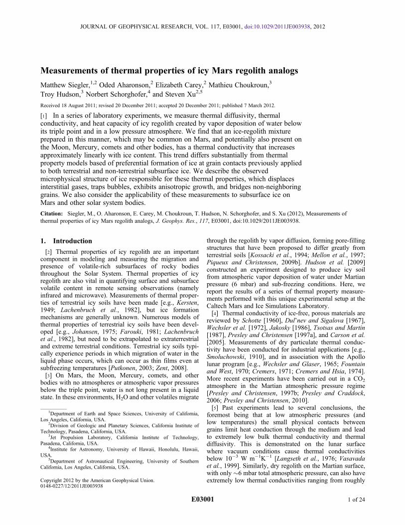
pletion of an experiment. To accomplish this, the column oficy soil was pushed out of the sample cup by using thebottom brass plate as a piston, then sliced into 5 mm thicksections. These sections were weighed before and afterbaking them for >24 h in a 130�C oven. Experiments pre-sented here use a multineedle, line source heat-pulse method[Campbell et al., 1991; Bristow et al., 1994], allowing for insitu measurement of thermal conductivity, thermal diffusiv-ity, and specific heat capacity. In this method, a single linearheater is briefly activated and then its cooling is monitoredto determine thermal conductivity of the surroundingmedium. The flow of heat to a neighboring, unheated needleis also monitored to extract thermal diffusivity and heatcapacity. The heat pulse is of short enough duration (�10 s)that it is assumed to have little effect on ice deposition in themedium. A probe with 11 horizontal needles remained in thesample medium during the experiment (Figure 2).[13] The 11 needles, each 60 mm long and 1 mm in

diameter, have an internal resistor of 1000 W m�1 runningthe length of the needle (Evanohm, custom constructed byEast 30 Sensors) and were typically pulsed with a constantvoltage of 6 � 0.01 V (outputting a total of 10.9 W m�1).The entire heat pulse is assumed delivered to the soil in ouranalysis. However, very low thermal conductivity measure-ments may be slightly affected by contact resistance betweenthe needles and the beads. With contact resistance, a fractionof the heat flows into the body of the probe instead of thesample. To decrease the chance of heat flow into the probe,the body was constructed of low thermal conductivity epoxyin a Teflon spine with the needles at 5 � 0.2 mm verticalspacing. The spine itself is a 15 mm � 15 mm � 70 mmhollowed channel with 11 holes. The needles each protrudedabout 46 mm from these holes and have an internal, E-typethermocouple at the center of the exposed portion of theneedle, 23 mm from the end. The probe is constructedpartially at 30-East Sensors and partially at Caltech. About2 mm of beads lay between the needle tips and the far wallof the sample cup, limiting conduction to the facing wall.The needle thermocouples are calibrated against a referenceT-type thermocouple in 0�C ice bath to correct for fluctua-tions within our data logger units (two Measurement Com-puting USB-TCs).[14] The heater, RH/RTD, lamp, and thermocouple wires

from the probe feed through the chamber wall individuallyand their measurement is digitized by National Instruments(DAQ-9172) and Measurement Computing (USB-1608FSand USB-TC) data loggers. Chamber temperature and pres-sure is controlled at approximately 3 s intervals while data

Figure 2. Schematic illustration of 11-needle thermal prop-erties probe. Each needle contains a heater and thermocou-ple. The brass base plate is in contact with a cold platechilled by liquid methanol, the surface is heated by the lamp.


3 of 24

from the needle thermocouples and heaters is recorded andtime-stamped once per second.

2.2. Regolith Simulants

[15] The ice filling experiment described here uses a bedof loosely packed (�43% porosity) glass spheres sieved tobetween 500 mm to 600 mm in diameter. The relatively largegrain size was chosen to allow for fast vapor diffusion, thespherical shape for ease of void space estimation and theo-retical modeling. The beads were chosen for their regularshape (see section 6) and to replicate the study of Presleyand Christensen [1997b]. Before each experiment, thebeads were washed in deionized water, resieved, and bakedat >130�C for at least one day.[16] The beads are approximately 72% SiO2, 14% Na2O,

and 9% CaO and should not have any strong surface wateradsorption properties (Jaygo Dragonite™ technical datasheet). This glass mixture has a solid density of about2750 kg m�3 and a solid thermal conductivity of about(1.5 � 10�3 (T-273) + 1.1277) W m�1 K�1 (for temperatureT in K, fit from Sciglass™ database).[17] We used a Setaram BT2.15 cryogenic calorimeter to

measure the heat capacity of the glass beads. This LN2-cooled calorimeter is equipped with a sample and a referencecell, which are housed inside the calorimetric block. Calvetelements (three-dimensional arrays of 64 thermocouples) areused to measure the heat flux to the cells with a precision of0.1 mW and use the reference cell as a differential, providinga direct measurement of the heat flux solely affecting thesample. Heat capacity is derived from the ratio of the heatflux delivered to the sample to sample mass as a function ofimposed heating rate.[18] The experimental results are plotted in Figure 3 and

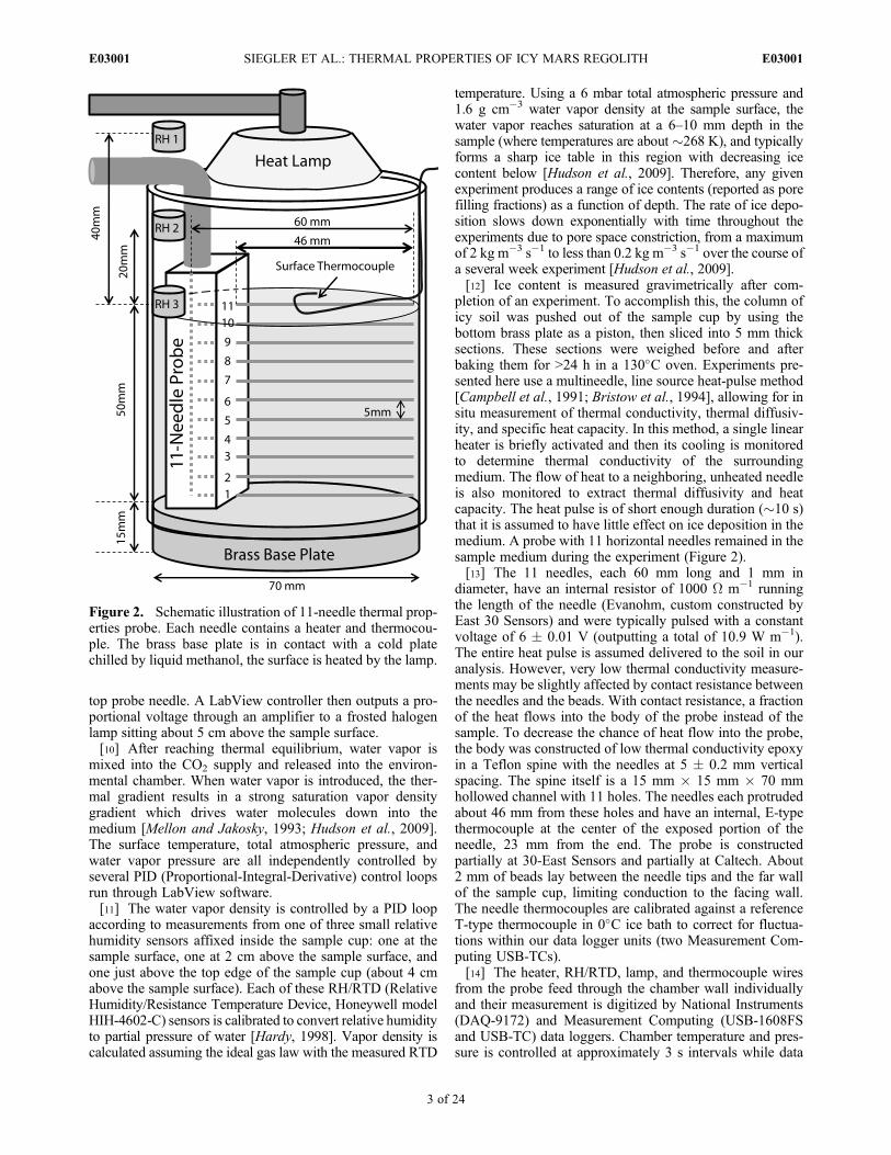
were conducted on a 12.1 g sample of glass beads heated ata rate of 0.2 K min�1 from 110 to 400 K. These results showa significant discrepancy (�10% above 200 K) from the fitto basalt samples presented by Winter and Saari [1969].

Parameters for equation (3) have been derived by nonlinearregression of our calorimeter data resulted in:

cdry ≈ ð1:28� 10�5T 3�1:19� 10�2T2þ5:14T� 110:4Þ J kg�1K�1

ð3Þ

valid between about 110 and 395 K. Equation (3) is used tocalculate cdry of our glass beads throughout this paper.[19] Further measurements were conducted with JSC

Mars-1 Regolith simulant [Allen et al., 1998; Seiferlin et al.,2008]. Though this simulant is designed as a spectral analogfor Mars, it can add confidence to the relevance of the glassbead thermal measurements to real Martian regolith which islikely to have basaltic composition and irregular shape. Forcomparison with glass bead measurements, the JSC Mars-1was also sieved between 500 and 600 mm and dried in asimilar manner. The sifted 500–600 mm JSC Mars-1 had ameasured a bulk density of 0.66 � 0.05 g cm�3 with anassumed particle density of 1.91 g cm�3 [Allen et al., 1998],resulting in a 65% porosity. We assign a 10% uncertainty ofour sieved JSC Mars-1solid particle density as we may haveremoved either a lighter or denser component. The solidconductivity of this basalt is expected to be approximately2 W m�1 K�1 [Langseth et al., 1976] and was not modeledto vary with temperature. This thermal conductivity shouldbe nearly twice that of the glass spheres, which will berevisited in section 5.5. The specific heat capacity repre-sented by equation (4) is based on past work applicable tobasalt minerals and used in this paper to best represent JSCMars-1 [Winter and Saari, 1969],

cdry basalt ≈ ð�34 T1=2 þ 8 T � 0:2 T3=2Þ J kg�1K�1: ð4Þ

As the beads are made of silica glass and were washed indeionized water, their surfaces may be hydrophobic relativeto JSC Mars-1 and other natural samples.

Figure 3. Measurement of specific heat capacity, c, and a 3rd-order fit (equation (3)) as compared to a fitto basaltic materials (equation (4)) [Winter and Saari, 1969, equation 16].


4 of 24

2.3. Experimental Procedure

[20] A set of vapor deposition experiments were per-formed under roughly identical conditions and stopped atvarious durations in order to span a range of ice contents.Table 1 presents a list of the experimental runs between0 and 570 h in length and the pore filling fractions achievedas well as several non-vapor deposited experiments.[21] Prior to each experiment roughly 280 g sample of

500–600 mm glass beads were baked in a 130�C oven for atleast 24 h and cooled, then poured into the sample cup, toform a 5 cm deep layer around the 11-needle probe. Thebottom of the brass base of the sample cup is coated with athin layer of silicon heat transfer compound, and then placedupon a cooling plate through which an external Neslab ULT95 chiller recirculates methanol at ��90�C.[22] The chamber is sealed, and then pumped down to

roughly 1 mbar for at least 8 h at room temperature prior tocooling the sample (which takes another 6–12 h to reachthermal equilibrium). Absolute atmospheric pressure is thencontrolled by a second PID loop to 6 � 0.2 mbar for theduration of the experiment. The PID loop controls a throttledbleed-in of dry or wet CO2 and a rough vacuum pump drawsexcess gas from the chamber. A small LACO cold trap (alsocooled by the methanol chiller) collects water vapor in thevacuum line. Once all the thermocouple temperatures arestable to within 0.1 K hr�1 the experiment is assumed inthermal equilibrium and a controlled flow CO2 and watervapor is allowed into the chamber (time zero in the quotedexperiment duration; see Table 1). During the experiment,water vapor density is controlled with a third PID loop(at 1.6 g cm�3 in the presented experiments) as measuredby the RH/RTD at the sample surface. Total atmosphericpressure is maintained at 6 � 0.2 mbar after the water vaporflow begins.[23] To measure thermal properties in situ, the 11 needles

of the probe are pulsed (out of order 1,7,2,8…, indexincreasing upward, to provide the largest distance betweenconsecutive pulses) with 6 V for 10 s each. The heat liber-ated per unit length per unit time, q′ (usually 10.9 W m�1), isdetermined within 5.5% from this input voltage and theheater specification. The uncertainty is mainly due to anunforeseen rise in resistance by �3 ohms as needle wiresaged, which is included as an error is our assumed q′. Pulseswere kept to 10 s so that the top needle (not used in thisanalysis) did not exceed 0�C, and all others did not exceed

�10�C as recommended by Putkonen [2003] who observeda dramatic change in thermal properties above this temper-ature, presumably due to thin films. Five minutes are givenbetween pulses to allow the heat to fully dissipate. Werequired at least three minutes of data after each pulse in fitsof heat pulses from a neighboring needle.[24] The experiment is then run in a stable environment

for a period of a few hours to nearly a month. Thermalproperties were measured at least once per hour at eachdepth. At the completion of an experiment the sample iscovered with aluminum foil and moved to a �10�C coldroom to be sampled as soon as possible. Within the coldroom, the sample is sliced into 5 mm thick discs, and thenweighed before and after a >24 h drying period in a 130�Coven [Hudson, 2009]. The mass loss between weighingcorresponds to the ice content in each sample layer. Thecorresponding thermophysical properties of each layer arederived from final heat pulses (within the last hour beforeremoval) of the needles adjacent to that layer.

3. Experimental Techniques

3.1. Line Source Heat-Pulse Method

[25] The 11-needle thermal probe utilizes both standardsingle and dual probe line source heat-pulse measurements.The single probe method [De Vries, 1952] uses a thin,epoxy-filled, hollow needle equipped with both an internalheater and thermocouple. When a brief pulse of electricity isapplied to the needle, the heat produced will flow into thesurrounding medium at a rate depending on the medium’sthermal properties. A higher thermal conductivity mediumwill cause the needle to reach a lower maximum temperatureduring heating and to cool more rapidly once the pulse hasceased.[26] De Vries [1952] developed a Green’s function solu-

tion (similar to that detailed in section 3.2) for a radial,cylindrically symmetric heat pulse (length t0) in whichthermal conductivity, diffusivity, and volumetric heatcapacity can be solved for assuming a homogeneous andisotropic medium:

DTðr; tÞ ¼ � q′

4pkrcEi

�r2

4kt

� �for 0 < t ≤ t0 ð5Þ

during the heat pulse, or

DTðr; tÞ ¼ q′

4pkrcEi

�r2

4kðt � t0Þ� �

� Ei�r2

4kt

� �� for t > to: ð6Þ

DT is the temperature change at a distance r from thesource, q′ the heat per unit length per unit time (generally�10.9 W m�1), and Ei is the Exponential Integral function

EiðxÞ ¼ Rx�∞

es=sð Þds.[27] Near the heat pulse source, r is small, and the Ei term

is approximated by Ei(x) ≈ g + ln(�x), where g is Euler’sconstant ≈0.5772. Bristow et al. [1994] denote the temper-ature offset with d and add an empirical time offset, tc.Equation (5) becomes

DT ≈q′

4plln t þ tcð Þ þ d 0 < t ≤ t0: ð7Þ

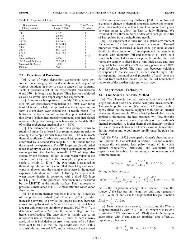
Table 1. Experimental Runs

Description orFilling Duration

Volumetric FillingRange, F (%)

Total PressureP, (mbar)

7 h 0–7.9 611 h 2.6–9.9 624 h 4.4–16.1 625.7 h 8.9–26.5 648.6 h 18.3–34.8 698 h 23.1–50.1 6220 h 41.8–69.9 6570 h 57.3–75.5 6Dry 0 1–12Saturated beads �100 6JSC Mars-1 269 hour 62.5–82.5 6Saturated JSC Mars-1 �100 6Pure ice N/A 6


5 of 24

In the same approximation, equation (6), the response afterthe pulse is complete, becomes

DT ≈q′

4plln t þ tcð Þ � ln t þ tc � toð Þ½ � þ d for t > t0: ð8Þ

[28] These quantities are solved for by a nonlinear regressionto the data. A principal shortcoming of the single probe methodis that it only results in a measurement of thermal conductivity,while thermal diffusivity and heat capacity of the mediumremain unmeasured. This can be seen in equations (7) and (8)where the quantity krc is rewritten as thermal conductivity, l.These equations assume that the thermal conductivity is iden-tical in all directions which, as discussed in section 3.2, may notnecessarily be true. Another shortcoming is the susceptibility ofthis measurement technique to contact resistance for shorttimescales (<�270 s, [Cull, 1978]), which can decrease theeffective heat, q′, released into the sample. This will increase themeasured value of l during heating (as heat is not allowed toescape the needle) and decrease the measured l during cooling(as heat is not deposited into the medium). Example heating/cooling data is shown in Figure 4.[29] In a dual-probe measurement one needle serves as a

heat source and a neighboring needle serves as a temperatureprobe. Therefore a nonlinear, piecewise fit to equation (5)and (6) can be used. Our method for deriving thermal

properties, which includes effects due to anisotropic heatflow, is discussed in section 3.2.

3.2. Line Source Heat-Pulse Methodin Anisotropic Medium

[30] As ice may preferentially grow along a thermal gra-dient, we generalize the equations used for single and dualprobe measurements of thermal conductivity to an aniso-tropic medium, where the conductivity in the vertical (z)direction may differ from that in a direction within the hor-izontal plane (x). The temperature and conductivity areassumed constant along the line source (y).[31] Due to the strong thermal gradient in the sample heat

will not only flow radially from each needle, but also verti-cally along the gradient. This requires a modification of thedual-probe fit. The gradient, dT/dz, defined as g, is assumedlinear (see Appendix A). For our analysis, the term gz isobtained from the time-averaged measured temperature fromthe needle prior to a heat pulse.[32] As first step, we seek the solution to the anisotropic,

i.e., k depends on direction, but spatially homogeneous, i.e.,k is independent of x and z, heat equation

∂T∂t

¼ kx∂2T∂x2

þ kz∂2T∂z2

; ð9Þ

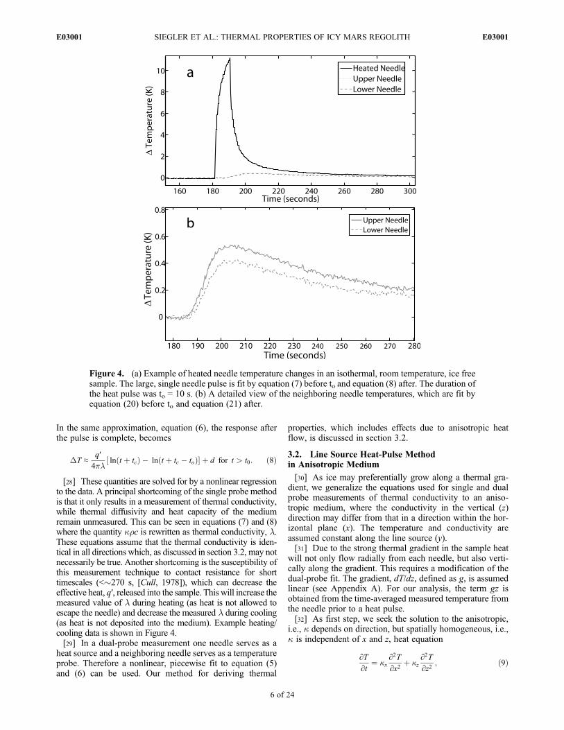
Figure 4. (a) Example of heated needle temperature changes in an isothermal, room temperature, ice freesample. The large, single needle pulse is fit by equation (7) before to and equation (8) after. The duration ofthe heat pulse was to = 10 s. (b) A detailed view of the neighboring needle temperatures, which are fit byequation (20) before to and equation (21) after.


6 of 24

for an instantaneous heat pulse at time t = 0 and an initiallylinear temperature profile. Because anisotropy in conduc-tivity is a result of preferential ice formation caused by thetemperature gradient, z is aligned with a principal axis of thediffusivity. It is convenient to write the solution in terms ofDT(x, z, t) = T(x, z, t) � gz, where the linear term gz satisfies(9) and also represents the initial condition, T(x, z, 0) = gz.While T(x, z, t) is the exact solution for an infinite domain, italso approximates the temperature distribution in the vicinityof the line source if the boundaries of the domain are farfrom the line source.[33] Using standard methods for partial differential equa-

tions, this solution is obtained as

DTðx; z; tÞ ¼ q

4prcffiffiffiffiffiffiffiffiffikxkz

ptexp � x2

4kxt� z2

4kzt

� �; ð10Þ

where q is the heat per unit length. The line source is locatedat (x, z) = (0, 0). It is easily verified that equation (10)satisfies the heat equation (9) and conserves the totalamount of heat (again per unit length),

rcZþ∞

�∞

dx

Zþ∞

�∞

dzDTðx; z; tÞ ¼ q: ð11Þ

[34] It also satisfies the desired boundary condition,DT = 0,infinitely far from the line source. Solution (10) is theGreen’s function of equation (9) for a source at (x, z) = (0, 0).The solution for a prolonged, finite heat pulse (subscript f )is obtained by integration of the Green’s function over time,

DTf ðx; z; tÞ ¼Z t

0

dt′DTðx; z; t � t′Þ ð12Þ

¼ � q′


p Ei � x2

4kxt� z2

4kzt

� �for 0 < t ≤ t0; ð13Þ

where Ei is again the Exponential Integral function and q′ isthe heat input per unit length per unit time. The solution for aheat pulse of finite duration, from t = 0 to t = t0, is obtainedby integration of the Green’s function over that period,

DTf ðx; z; tÞ ¼Zt00

dt′DTðx; z; t � t′Þ ð14Þ

¼ q′


p"Ei � x2

4kx t � t0ð Þ �z2

4kz t � t0ð Þ� �

� Ei � x2

4kxt� z2

4kzt

� �#for t > t0: ð15Þ

Again, it can be verified that equations (13) and (15) satisfy(9) and, respectively,

rcZþ∞

�∞

dx

Zþ∞

�∞

dzDTf ðx; z; tÞ ¼ q′t for 0 < t ≤ t0 ð16Þ

and

rcZþ∞

�∞

dx

Zþ∞

�∞

dzDTf ðx; z; tÞ ¼ q′t0 for t > t0: ð17Þ

[35] From equations (13) and (15) we obtain the relationneeded to invert the single probe measurements for small xand z,

DTf ¼ q′


p lnðtÞ þ d for 0 < t ≤ t0 ð18Þ

and

DTf ¼ q′


p lnt

t � t0ð Þ for t > t0: ð19Þ

This provides measurement of rcffiffiffiffiffiffiffiffiffikxkz

p ¼ ffiffiffiffiffiffiffiffiffilxlz

p, which is

the geometrically averaged conductivity. The relevantequations for dual probe measurements are

DTf ð0; z; tÞ ¼ � q′


p Ei � z2

4kzt

� �for 0 < t ≤ t0 ð20Þ

and

DTf ð0; z; tÞ ¼ q′


p Ei � z2

4kz t � t0ð Þ� �

� Ei � z2

4kzt

� �� for t > t0: ð21Þ

[36] The time and distance dependence provides mea-surement of kz; the prefactor combined with kz and q′ pro-vides rc

ffiffiffiffiffiffiffiffiffiffiffiffikx=kz

p. Only in the isotropic case does it provide a

separate measurement of rc. The measurement of rcffiffiffiffiffiffiffiffiffiffiffiffikx=kz

pdepends directly on knowledge of heat input, q′, and thus issensitive to any contact resistance and heat loss to the bodyof the probe. The thermal diffusivity, kz, is unaffected byerrors in q′, as it falls within the Exponent Integral inequations (20) and (21). Error analysis of the nonlinear fitto (20) and (21) is detailed in Appendix A.

3.3. Data Analysis Methods

[37] Heated needle data during the heat pulse are generallytoo coarse (only 10 data points at a collection rate of 1 persecond) for a robust fit, so thermal conductivity (as derivedfrom the single needle measurement) is obtained by a non-linear fit of equation (8), to the cooling trend of the needle.The single-needle method inherently samples the entiremedium around the needle and is not sensitive to possiblyanisotropic heat flow (see section 3.2). This method is alsomore susceptible to resistance caused by poor contactbetween the needle and the surrounding medium [Cull,1978], mimicking a change in thermal properties. Both ofthese errors directly effect the heat input to the sample, q′ inequations (7) and (8), and are not separated here.[38] The temperature change at a needle above and below

a pulsed needle can be used to determine the thermal diffu-sivity of the medium between the needles. The temperatureincrease at the neighboring needle was less than 1 K(Figure 4b), so a sensitive thermocouple is necessary fora good fit (the E-type thermocouples here had a roughly


7 of 24

0.02 K error). A fit to the next farthest needle (10 mm away)proved impossible without exceeding 263 K at some needle.[39] The effect of the thermal gradient was removed by

subtracting a time averaged temperature of the sensing nee-dle for the 100 s prior to the heat pulse. Then a nonlinear fitwas computed to the temperature profile using equation (20)for times t < to and equation (21) for t ≥ to. This allows aseparate estimate of kz and rc


p, or k and rc if the

medium is isotropic. Needles 1 and 11 (top and bottom)were not used for the thermal properties analysis due to theirproximity to the sample boundaries. The horizontal samplesize is a factor of a few larger than the characteristic lengthscale for diffusion of heat (for typical diffusivities <1 �10�6 m s�2) during the�3–5 min of data used for the fits, soedge effects are neglected.[40] The derived thermal property values at each needle

can then be directly associated with the gravimetricallymeasured ice fraction of the medium most closely repre-sented by that needle. Ice content is measured at the end of agiven experiment, so only conductivity values from the lasthours (last pulse of each needle) from each experiment arepresented here. These results may be used to estimate icecontent in situ in the future.[41] At the end of an experiment, the chamber is returned

to room pressure and the sample container is immediatelymoved to the 263 K sampling room. The brass bottom of thesample is designed to be incrementally pushed up throughthe sample cup to allow thin layers to be either brushed orsawed (in the case of ice cemented soils) for gravimetricanalysis. Horizontal slices of the sample, taken at 5 mmintervals, and all loose material are funneled into glass bea-kers and immediately weighed to give the total layer mass,mt. Material may be sampled at this point for microscopicdocumentation (such material is not included in mt, but isnegligible compared to the total mass). The beakers are thenbaked at 390 K for at least 24 h, cooled, then weighted toobtain the dry sample mass, ms.[42] The ice content can be expressed as the pore filling

fraction F = s/s0, where s is the ice density in the availablevolume, s = rbulk(mt/ms � 1), and s0 is the maximum pos-sible density of ice (filled pores), s0 = �0rice. The bulkdensity of the dry medium, rbulk, is 1570 � 10 kg m�3 forglass beads and rice is taken as 918 kg m�3 [Lide, 2003].

4. Theoretical Expectations

4.1. Modes of Heat Transport in Porous Media

[43] The effective thermal conductivity of a porousmedium is generally subdivided into three parallel heatpaths: lbs, the conduction through the bulk solid (whichincludes grain to grain contact resistance), lg, the conduc-tion via the pore space gas, and lr, the radiative conductionthrough the pore space [Wechsler et al., 1972; Jakosky,1986]. These same conceptual divisions apply to thermaldiffusivity, but are discussed in terms of conductivity herefor comparison with prior literature.[44] In particulate media, grain contact points create a bot-

tleneck for heat flow, and thus lbs can be very small. Thereforethe thermal conductivity of solid rock (or ice), ls, can beorders of magnitude higher than lbs of the same material. lbsdepends highly on grain size [Presley and Christensen, 1997b;

Slavin et al., 2002; Piqueux and Christensen, 2009a], grainroughness [Bahrami et al., 2006], shape, and particle mixture(Presley and Craddock [2006], including cemented grains[Presley and Christensen, 2010; Piqueux and Christensen,2009b]). At temperatures below those tested in our lab, lsmay have a strong temperature dependence as phonon heattransfer within the solid grains is inhibited. Throughout thispaper lbs is often combined with lg as ldry.[45] Presley and Christensen [1997b] found the gas con-

ductivity, lg, to have a P0.6 dependence of conductivity when

gases are confined in a fine grained porous medium. Thisdiffers from a free gas, where thermal conductivity is pres-sure independent due to the fact that at low pressure there arefewer molecules to transfer heat, but the mean free path ofeach of the particles increases. In a porous medium, thermalconductivity drops with decreasing pressure as the mean freepath cannot increase beyond the diameter of a pore.[46] In addition to gas collisions, deposition of a water

vapor molecule on a grain surface can also transfer heat. Inour experiment, the fluxes associated with advected heat bywater molecules and latent heat of their condensation aresmall compared to the heat flux from needle pulses andhence are neglected. The fastest observed deposition rate is2 � 10�3 kg m�3 s�1, about 2–4 times the average rate[Hudson et al., 2009], and a latent heat of deposition of2,585 kJ kg�1 (at 237 K) is assumed. This fastest observeddeposition is equivalent to a pulse of 0.96 W m�1, less than9% of the heat delivered by a typical needle measurement,excluding any heat lost upon sublimation which wouldreduce this value. The time-integrated latent heat transferwas found to cause the overall thermal gradient to be slightlynonlinear for the highest deposition rates [Hudson et al.,2009], but we do not believe this affected individualmeasurements.[47] At high temperatures radiative conduction, lr, can

dominate over lbs. The radiative component of conductionvaries as T3 [Schotte, 1960; Watson, 1964; Cuzzi, 1972].This T3 relation follows from a balance of the radiative heatflow (radiating proportional to T 4) between two grain sur-faces. For 1 mm sized particles, radiation does not become aconsiderable factor in heat transport until a temperature ofabout 400�C (1500�C for 0.1 mm) [Schotte, 1960] so it isnegligible for icy regolith.

4.2. Addition of Ice to a Porous Media

[48] Assuming slow deposition, the effect of ice on heattransport is primarily due to the geometry of the ice connec-tions within pores. Ice introduced into a dry porous mediumby vapor transport has been theorized to first form at graincontacts [Mellon et al., 1997], the concave meeting pointof any two grains. The inward curvature at these contactscauses a lower saturation vapor density in the gas above thesurface, similar to the process of evaporation-condensationsintering [Hobbs and Mason, 1964]. Through its influenceon the cross section available for conduction, such sinteredice necks may rapidly increase thermal conductivity withrelatively little ice cement [Mellon et al., 1997; Piqueuxand Christensen, 2009b]. If ice instead fills the voidsbetween grains homogeneously, one might expect smallerincrease in conductivity with ice content. A lower conduc-tivity trend of this sort is observed in thermal properties


8 of 24

measurements of permafrost on Earth [Johansen, 1975;Farouki, 1981; Lachenbruch et al., 1982] that have experi-enced a liquid state (or temperatures near 0�C) in the recentpast.[49] Mellon et al. [1997] and later Piqueux and

Christensen [2009b] applied the sintering theory to ice/cement welded soils on the Martian surface. The curvature ofthe grain causes a local vapor density gradient with a higherdensity above the convex surface and a low density above thegrain contact. Thus, the shape of the grain itself creates agradient in chemical potential between the overall grainsurface and grain contact points. In this theory, explored inmore detail in section 6, this density gradient acts as a force todrive molecules toward the contacts and form necks which,in our case being made of highly conductive ice, will greatlyincrease the solid conductivity of the material.[50] Assuming ice deposits at these low free-energy con-

tacts, one can directly relate the diameter of the conductiveneck to its volume. Hobbs and Mason [1964] solve the neckgeometry as: Vneck = p2x4/(4rgrain), Aneck = p2x3/rgrain, andrneck = x2/(2rgrain) where Vneck is the neck volume, Aneck isthe surface area of the neck exposed to gas, and rneck is theradius of curvature of the neck. rgrain refers to the grainradius and x to the cross-sectional neck radius. The cross-sectional area of the neck (the conduction pathway) is px2.Using this geometry,Mellon et al. [1997] recognized that thefractional area of the pore space which ice adds to heatconduction, fA, can be approximately represented by thesquare root of the fractional volume of the pore space takenup by ice, such that fA =

ffiffiffiffiF

p. This model treats the heat

conduction across a pore as

lp ¼ ð1� fAÞlp0 þ fAlice: ð22Þ

Adding this contribution in parallel, the bulk conductivitybehaves as

l ¼ lslp

ð1� �0Þlp þ �0ls; ð23Þ

where ls is the conductivity of the grain material and lp isthe conduction across the pores. lp0, the conduction acrossthe pores with zero ice content, is found by inverting thisequation and setting lp to lp0 (which is essentially lg) andsetting l equal to ldry, the bulk thermal conductivity of theice-free beads. In this paper, ldry is taken to be 0.068 �0.011 W m�1K�1 at 6 mbar, in agreement with our mea-surements at 298 K. Measurements were also taken at lowertemperatures, but a discernable trend in thermal conductivitywas not found within error. The thermal conductivity of ice,which varies strongly with temperature, lice(T), is taken tobe (488.19/T + 0.4685) W m�1 K�1 [Hobbs, 1974].[51] Multiple icy soil conductivity models exist for ter-

restrial applications. They are typically obtained fromempirical fits to data rather than physical models [Sass et al.,1971; Johansen, 1975; Farouki, 1981; Lachenbruch et al.,1982]. As terrestrial permafrost is invariably undergoing asuccession of freeze-thaw cycles, these models may beinapplicable to vapor derived ice. Indeed, warmer periods inwhich water is liquid will allow surface tension to dominateice structure. In addition, such empirical models could breakdown in situations of low pressures and temperatures.

[52] Fitting data from Kersten [1949], Johansen [1975]adopted a weighted geometric mean model for ice withentirely filled pores (F = 1),

lðF¼1Þ ¼ l1��0s l�0

ice: ð24Þ

Johansen’s original model included a third term for liquidwater, which was present in the Kersten data, but has beenremoved here as by Farouki [1981]. The thermal conduc-tivity of partially filled, icy regolith can then be written asthe linear interpolation,

l ¼ ðlðF¼1Þ � ldryÞF þ ldry: ð25Þ

This model implies that terrestrial permafrost structures aredominated by nucleation sites other than grain contact points.[53] Another simple model for ice is a volumetric mix of

ice and soil properties, as occurs with density dependentproperties like volumetric heat capacity. This results in therelation

l ¼ ldry þ �0liceF; ð26Þ

which is called the volumetric mixing model throughout thispaper. However, predictions by this model will likely breakdown at high ice contents for which the conduction will nolonger be dominated by grain contact points, but by heattransfer through the bulk solids.[54] A gas component can be added to any of these models

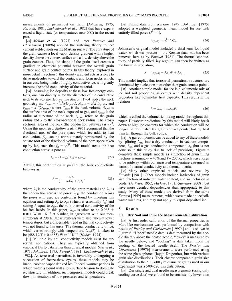
by splitting ldry into a dry conduction in vacuum compo-nent, lbs, and a gas conduction component, lg (but is notdone so in this study due to lack of precision). Figure 5compares these simple models as a function of grain fillingfraction (assuming �0 = 43% and T = 237 K, which was chosento be midway within our measured temperature extremes) interms of thermal conductivity and thermal inertia.[55] Many other empirical models are reviewed by

Farouki [1981]. Other models include intricacies of grainsize, fraction of unfrozen water content, and air inclusion invoids [De Vries, 1952; Mickley, 1951; Gavriliev, 2008], buthave more detailed dependencies than appropriate to thisstudy. Many of these models are derived from the sameKersten [1949] measurements, which were made on ice/soil/water mixtures, and may not apply to vapor deposited ice.

5. Results

5.1. Dry Soil and Pure Ice Measurements/Calibration

[56] A first order calibration of the thermal properties inMars-like environment was performed by comparison withresults of Presley and Christensen [1997b] and is shown inFigure 6. “Upper” needle data is data measured by the nee-dle directly above the heated needle, “lower” is measured bythe needle below, and “cooling” is data taken from thecooling of the heated needle itself. The Presley andChristensen [1997b] measurements were performed usingthe same glass spheres (Jaygo Dragonite), but with variousgrain size distributions. Their closest comparable grain sizedistribution to the 500–600 mm diameter grains used in ourexperiment was a 500–520 mm distribution.[57] Our single and dual needle measurements (using only

cooling curve data) were found to be consistently lower than


9 of 24

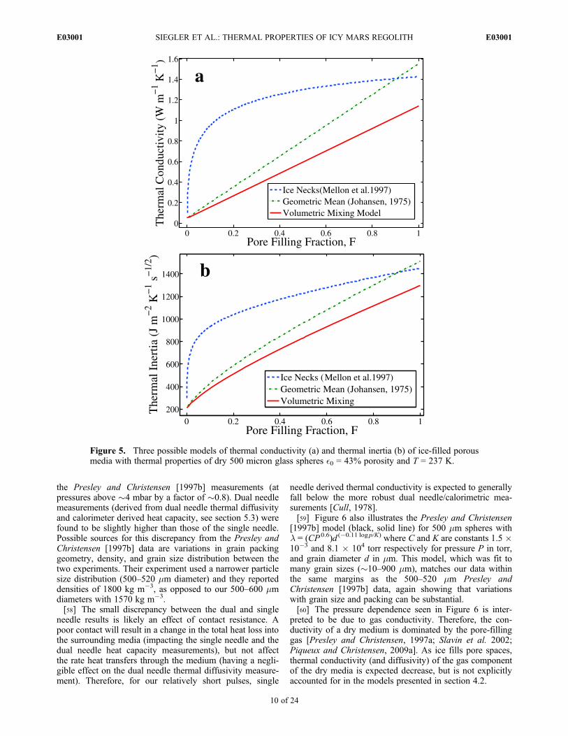
the Presley and Christensen [1997b] measurements (atpressures above �4 mbar by a factor of �0.8). Dual needlemeasurements (derived from dual needle thermal diffusivityand calorimeter derived heat capacity, see section 5.3) werefound to be slightly higher than those of the single needle.Possible sources for this discrepancy from the Presley andChristensen [1997b] data are variations in grain packinggeometry, density, and grain size distribution between thetwo experiments. Their experiment used a narrower particlesize distribution (500–520 mm diameter) and they reporteddensities of 1800 kg m�3, as opposed to our 500–600 mmdiameters with 1570 kg m�3.[58] The small discrepancy between the dual and single

needle results is likely an effect of contact resistance. Apoor contact will result in a change in the total heat loss intothe surrounding media (impacting the single needle and thedual needle heat capacity measurements), but not affectthe rate heat transfers through the medium (having a negli-gible effect on the dual needle thermal diffusivity measure-ment). Therefore, for our relatively short pulses, single

needle derived thermal conductivity is expected to generallyfall below the more robust dual needle/calorimetric mea-surements [Cull, 1978].[59] Figure 6 also illustrates the Presley and Christensen

[1997b] model (black, solid line) for 500 mm spheres withl = (CP0.6)d (�0.11 logp/K) where C and K are constants 1.5 �10�3 and 8.1 � 104 torr respectively for pressure P in torr,and grain diameter d in mm. This model, which was fit tomany grain sizes (�10–900 mm), matches our data withinthe same margins as the 500–520 mm Presley andChristensen [1997b] data, again showing that variationswith grain size and packing can be substantial.[60] The pressure dependence seen in Figure 6 is inter-

preted to be due to gas conductivity. Therefore, the con-ductivity of a dry medium is dominated by the pore-fillinggas [Presley and Christensen, 1997a; Slavin et al. 2002;Piqueux and Christensen, 2009a]. As ice fills pore spaces,thermal conductivity (and diffusivity) of the gas componentof the dry media is expected decrease, but is not explicitlyaccounted for in the models presented in section 4.2.

Figure 5. Three possible models of thermal conductivity (a) and thermal inertia (b) of ice-filled porousmedia with thermal properties of dry 500 micron glass spheres �0 = 43% porosity and T = 237 K.


10 of 24

[61] Pure ice represents another point of calibration. Anice sample was made by freezing water from the bottom ofthe sample upward, maintaining an ice free surface with theheating lamp to allow trapped gas to escape. Maintaining theice at a temperature of �259 K, both dual and single needlemeasurements of thermal conductivity are found to approx-imately match the theoretical value of 2.34 W m�1K�1

[Hobbs, 1974] with 2.41 � 0.41 W m�1K�1 and 2.35 �0.42 W m�1K�1 respectively. Volumetric heat capacity ofice also agree (with theoretical value 1.865� 106 J kg�1K�1

[Hobbs, 1974]) at 1.59 � 106 � 0.32 � 106 J kg�1K�1.

Thermal diffusivity (with theoretical value 1.26 � 10�6 m2

s�1) is measured as 1.29 � 10�6 � 0.22 � 10�6 m2 s�1.These agreements imply contact resistance is not a factorwhen good thermal contact between the needles and themedium (in this case the ice) exists. Once enough ice isemplaced, the vapor-filled samples are conjectured to be ingood thermal contact with the needles.[62] Experiments were run for various durations (see

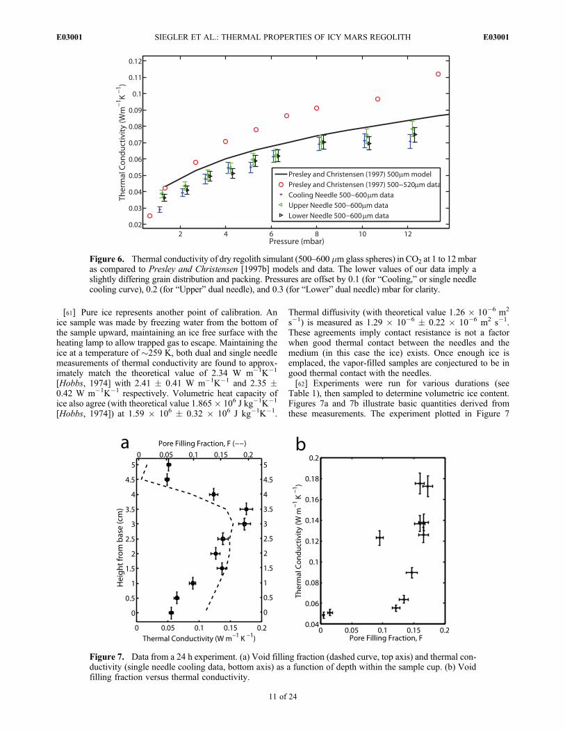
Table 1), then sampled to determine volumetric ice content.Figures 7a and 7b illustrate basic quantities derived fromthese measurements. The experiment plotted in Figure 7

Figure 6. Thermal conductivity of dry regolith simulant (500–600 mm glass spheres) in CO2 at 1 to 12mbaras compared to Presley and Christensen [1997b] models and data. The lower values of our data imply aslightly differing grain distribution and packing. Pressures are offset by 0.1 (for “Cooling,” or single needlecooling curve), 0.2 (for “Upper” dual needle), and 0.3 (for “Lower” dual needle) mbar for clarity.

Figure 7. Data from a 24 h experiment. (a) Void filling fraction (dashed curve, top axis) and thermal con-ductivity (single needle cooling data, bottom axis) as a function of depth within the sample cup. (b) Voidfilling fraction versus thermal conductivity.


11 of 24

(24 h in length) shows single needle derived conductivity.Individual measurements show an upward trend in conduc-tivity for higher ice content data (Figure 7a). Figure 7billustrates how thermal conductivity and volumetric fillingfraction vary with depth. There is a general increase inthermal conductivity with ice content, but increasing farmore rapidly in more ice-rich layers.

5.2. Dual Needle Data: Thermal Diffusivityand Nominal Volumetric Heat Capacity

[63] Dual needle measurements can be used to derivethermal diffusivity in the vertical direction, kz, and nominalvolumetric heat capacity, rc


p(which assumes no

contact resistance). kz, is nearly unaffected by anisotropyand contact resistance, but like the single needle data rc�ffiffiffiffiffiffiffiffiffiffiffiffikx=kz

pis intimately intertwined with anisotropic ice

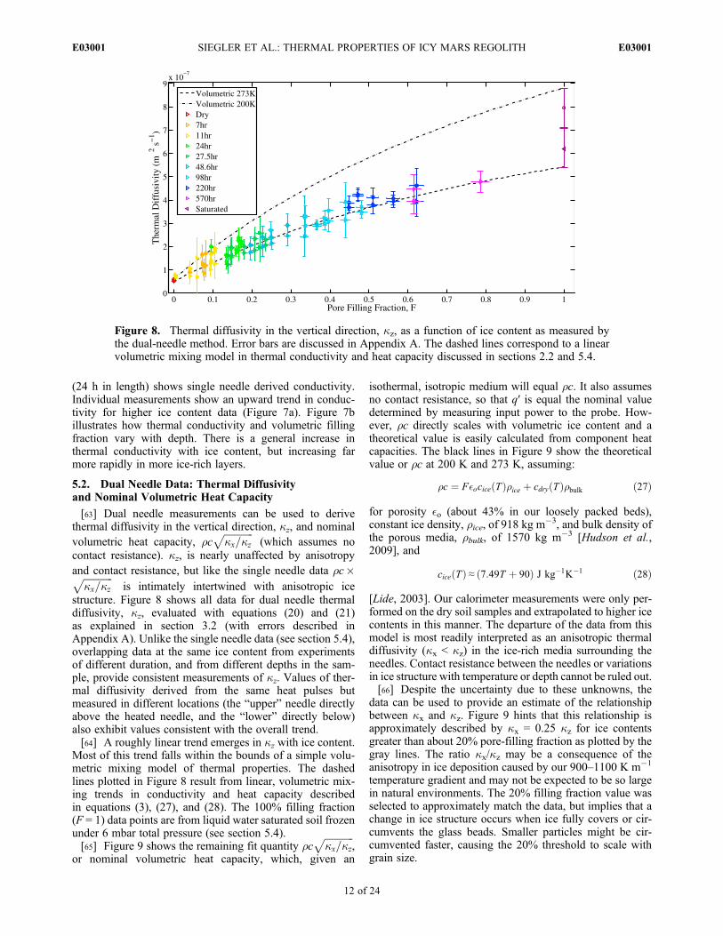
structure. Figure 8 shows all data for dual needle thermaldiffusivity, kz, evaluated with equations (20) and (21)as explained in section 3.2 (with errors described inAppendix A). Unlike the single needle data (see section 5.4),overlapping data at the same ice content from experimentsof different duration, and from different depths in the sam-ple, provide consistent measurements of kz. Values of ther-mal diffusivity derived from the same heat pulses butmeasured in different locations (the “upper” needle directlyabove the heated needle, and the “lower” directly below)also exhibit values consistent with the overall trend.[64] A roughly linear trend emerges in kz with ice content.

Most of this trend falls within the bounds of a simple volu-metric mixing model of thermal properties. The dashedlines plotted in Figure 8 result from linear, volumetric mix-ing trends in conductivity and heat capacity describedin equations (3), (27), and (28). The 100% filling fraction(F = 1) data points are from liquid water saturated soil frozenunder 6 mbar total pressure (see section 5.4).[65] Figure 9 shows the remaining fit quantity rc


p,

or nominal volumetric heat capacity, which, given an

isothermal, isotropic medium will equal rc. It also assumesno contact resistance, so that q′ is equal the nominal valuedetermined by measuring input power to the probe. How-ever, rc directly scales with volumetric ice content and atheoretical value is easily calculated from component heatcapacities. The black lines in Figure 9 show the theoreticalvalue or rc at 200 K and 273 K, assuming:

rc ¼ F�ocice Tð Þrice þ cdryðTÞrbulk ð27Þ

for porosity �o (about 43% in our loosely packed beds),constant ice density, rice, of 918 kg m

�3, and bulk density ofthe porous media, rbulk, of 1570 kg m�3 [Hudson et al.,2009], and

ciceðTÞ ≈ ð7:49T þ 90Þ J kg�1K�1 ð28Þ

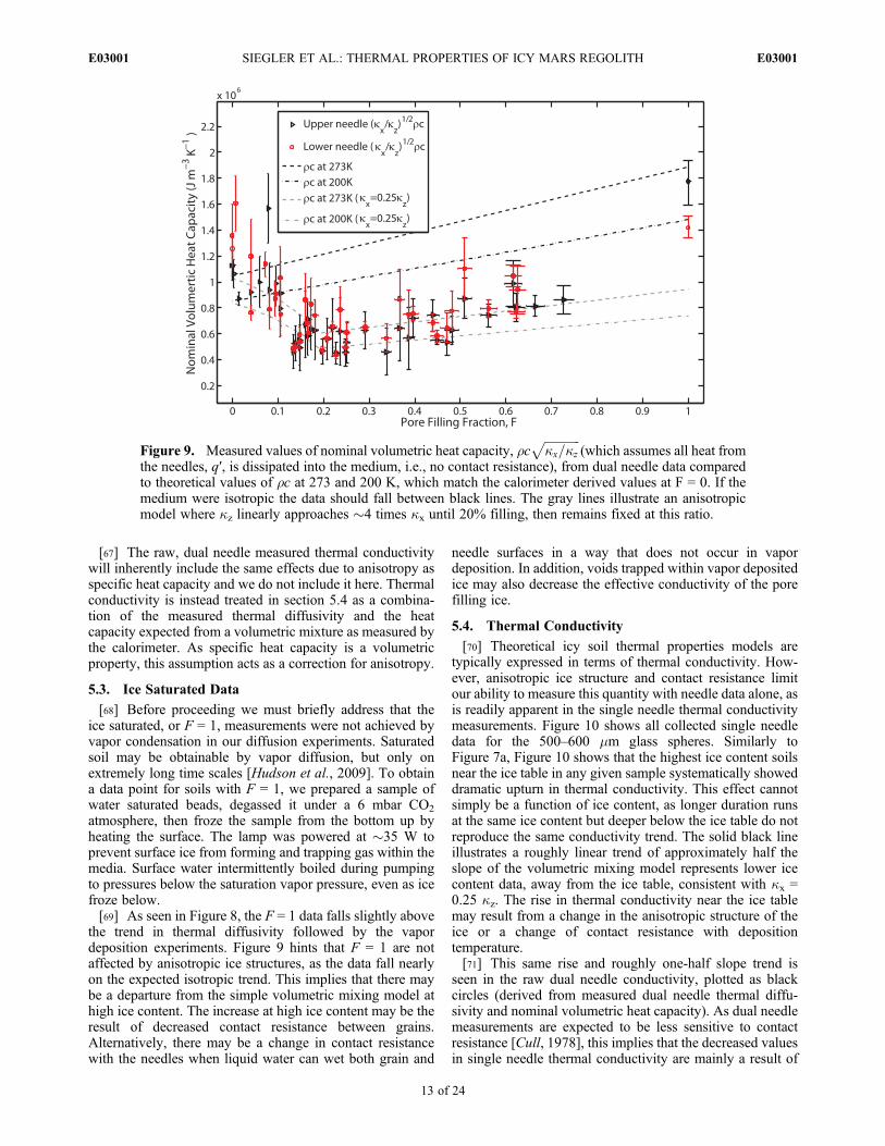
[Lide, 2003]. Our calorimeter measurements were only per-formed on the dry soil samples and extrapolated to higher icecontents in this manner. The departure of the data from thismodel is most readily interpreted as an anisotropic thermaldiffusivity (kx < kz) in the ice-rich media surrounding theneedles. Contact resistance between the needles or variationsin ice structure with temperature or depth cannot be ruled out.[66] Despite the uncertainty due to these unknowns, the

data can be used to provide an estimate of the relationshipbetween kx and kz. Figure 9 hints that this relationship isapproximately described by kx = 0.25 kz for ice contentsgreater than about 20% pore-filling fraction as plotted by thegray lines. The ratio kx/kz may be a consequence of theanisotropy in ice deposition caused by our 900–1100 K m�1

temperature gradient and may not be expected to be so largein natural environments. The 20% filling fraction value wasselected to approximately match the data, but implies that achange in ice structure occurs when ice fully covers or cir-cumvents the glass beads. Smaller particles might be cir-cumvented faster, causing the 20% threshold to scale withgrain size.

Figure 8. Thermal diffusivity in the vertical direction, kz, as a function of ice content as measured bythe dual-needle method. Error bars are discussed in Appendix A. The dashed lines correspond to a linearvolumetric mixing model in thermal conductivity and heat capacity discussed in sections 2.2 and 5.4.


12 of 24

[67] The raw, dual needle measured thermal conductivitywill inherently include the same effects due to anisotropy asspecific heat capacity and we do not include it here. Thermalconductivity is instead treated in section 5.4 as a combina-tion of the measured thermal diffusivity and the heatcapacity expected from a volumetric mixture as measured bythe calorimeter. As specific heat capacity is a volumetricproperty, this assumption acts as a correction for anisotropy.

5.3. Ice Saturated Data

[68] Before proceeding we must briefly address that theice saturated, or F = 1, measurements were not achieved byvapor condensation in our diffusion experiments. Saturatedsoil may be obtainable by vapor diffusion, but only onextremely long time scales [Hudson et al., 2009]. To obtaina data point for soils with F = 1, we prepared a sample ofwater saturated beads, degassed it under a 6 mbar CO2

atmosphere, then froze the sample from the bottom up byheating the surface. The lamp was powered at �35 W toprevent surface ice from forming and trapping gas within themedia. Surface water intermittently boiled during pumpingto pressures below the saturation vapor pressure, even as icefroze below.[69] As seen in Figure 8, the F = 1 data falls slightly above

the trend in thermal diffusivity followed by the vapordeposition experiments. Figure 9 hints that F = 1 are notaffected by anisotropic ice structures, as the data fall nearlyon the expected isotropic trend. This implies that there maybe a departure from the simple volumetric mixing model athigh ice content. The increase at high ice content may be theresult of decreased contact resistance between grains.Alternatively, there may be a change in contact resistancewith the needles when liquid water can wet both grain and

needle surfaces in a way that does not occur in vapordeposition. In addition, voids trapped within vapor depositedice may also decrease the effective conductivity of the porefilling ice.

5.4. Thermal Conductivity

[70] Theoretical icy soil thermal properties models aretypically expressed in terms of thermal conductivity. How-ever, anisotropic ice structure and contact resistance limitour ability to measure this quantity with needle data alone, asis readily apparent in the single needle thermal conductivitymeasurements. Figure 10 shows all collected single needledata for the 500–600 mm glass spheres. Similarly toFigure 7a, Figure 10 shows that the highest ice content soilsnear the ice table in any given sample systematically showeddramatic upturn in thermal conductivity. This effect cannotsimply be a function of ice content, as longer duration runsat the same ice content but deeper below the ice table do notreproduce the same conductivity trend. The solid black lineillustrates a roughly linear trend of approximately half theslope of the volumetric mixing model represents lower icecontent data, away from the ice table, consistent with kx =0.25 kz. The rise in thermal conductivity near the ice tablemay result from a change in the anisotropic structure of theice or a change of contact resistance with depositiontemperature.[71] This same rise and roughly one-half slope trend is

seen in the raw dual needle conductivity, plotted as blackcircles (derived from measured dual needle thermal diffu-sivity and nominal volumetric heat capacity). As dual needlemeasurements are expected to be less sensitive to contactresistance [Cull, 1978], this implies that the decreased valuesin single needle thermal conductivity are mainly a result of

Figure 9. Measured values of nominal volumetric heat capacity, rcffiffiffiffiffiffiffiffiffiffiffiffikx=kz

p(which assumes all heat from

the needles, q′, is dissipated into the medium, i.e., no contact resistance), from dual needle data comparedto theoretical values of rc at 273 and 200 K, which match the calorimeter derived values at F = 0. If themedium were isotropic the data should fall between black lines. The gray lines illustrate an anisotropicmodel where kz linearly approaches �4 times kx until 20% filling, then remains fixed at this ratio.


13 of 24

anisotropic ice structure. The near overlap of these two datasets supports, but does not guarantee, that we are measuringanisotropic thermal structure and not contact resistance withthe single needle measurement.[72] However, the ambiguity introduced by anisotropic

thermal structure and contact resistance can be cir-cumvented. Since volumetric ice content is measured sepa-rately, one can use volumetric heat capacity as measuredfrom the calorimeter, rc, to calculate the quantity lz = kzrc(thermal conductivity in the vertical direction). As discussedin section 5.2, the volumetric heat capacity can be reliablycalculated from volumetric mixing (equation (27)) and the

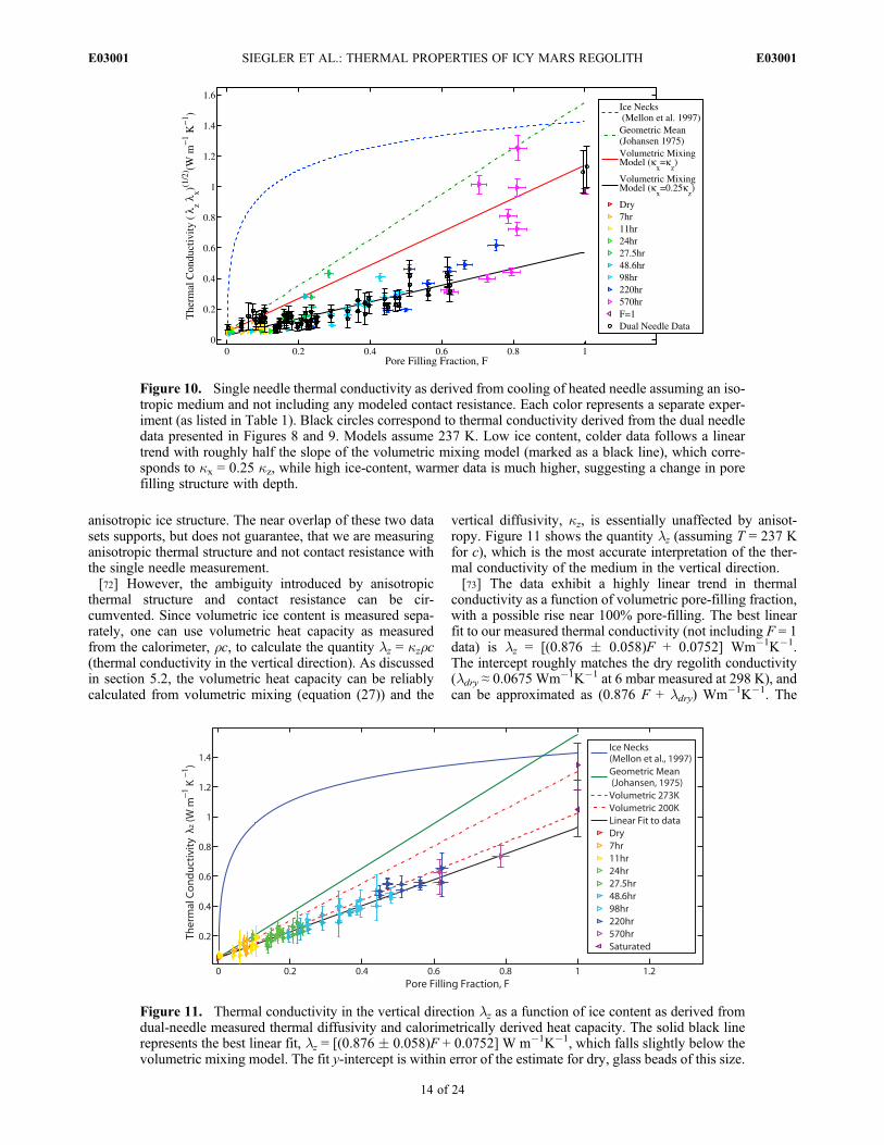
vertical diffusivity, kz, is essentially unaffected by anisot-ropy. Figure 11 shows the quantity lz (assuming T = 237 Kfor c), which is the most accurate interpretation of the ther-mal conductivity of the medium in the vertical direction.[73] The data exhibit a highly linear trend in thermal

conductivity as a function of volumetric pore-filling fraction,with a possible rise near 100% pore-filling. The best linearfit to our measured thermal conductivity (not including F = 1data) is lz = [(0.876 � 0.058)F + 0.0752] Wm�1K�1.The intercept roughly matches the dry regolith conductivity(ldry ≈ 0.0675 Wm�1K�1 at 6 mbar measured at 298 K), andcan be approximated as (0.876 F + ldry) Wm�1K�1. The

Figure 10. Single needle thermal conductivity as derived from cooling of heated needle assuming an iso-tropic medium and not including any modeled contact resistance. Each color represents a separate exper-iment (as listed in Table 1). Black circles correspond to thermal conductivity derived from the dual needledata presented in Figures 8 and 9. Models assume 237 K. Low ice content, colder data follows a lineartrend with roughly half the slope of the volumetric mixing model (marked as a black line), which corre-sponds to kx = 0.25 kz, while high ice-content, warmer data is much higher, suggesting a change in porefilling structure with depth.

Figure 11. Thermal conductivity in the vertical direction lz as a function of ice content as derived fromdual-needle measured thermal diffusivity and calorimetrically derived heat capacity. The solid black linerepresents the best linear fit, lz = [(0.876 � 0.058)F + 0.0752] W m�1K�1, which falls slightly below thevolumetric mixing model. The fit y-intercept is within error of the estimate for dry, glass beads of this size.


14 of 24

measured values fall at roughly 61% the slope of the value alinear Johansen [1975] model and 80% that of the volu-metric mixing model is as described in section 4 (at 237 K).A trend line including the F = 1 data is best fit by (1.122 F +0.0246) Wm�1K�1 (which would be �75% of the Johansenmodel and �103% that of the volumetric model).[74] One clear, and perhaps surprising, result is that our

laboratory data shows little resemblance to the expectedconductivity of the ice neck model. This is of particularimportance to thermal modeling of the Martian environment,where past work typically relied on the assumption thatvapor deposition will result in ice necks [Mellon et al., 1997;Piqueux and Christensen, 2009b]. The laboratory dataimplies that our system is not forming sintered ice necksbetween neighboring grains. Why this occurred, andwhether this is also expected to occur on Mars is discussedin further detail in sections 6 and 7.

5.5. JSC Mars-1 Measurements

[75] Of the models presented, the volumetric mixingmodel best represents our experimental data. However, datataken in saturated glass spheres, with an average conduc-tivity of 1.31 W m�1K�1, fall close to the Johansen geo-metric mean model (1.54 W m�1K�1), implying that thesoil-independent, volumetric mixing model breaks down athigh ice content (it predicts 1.10 W m�1K�1). This suggeststhe best fit model might be one resembling the volumetricmixing model at low to moderate ice contents, but increasingtoward the geometric model at greater than �80% porefilling when grains become fully interconnected.[76] A second hypothesis could be that the geometric

mean model [Johansen, 1975] best explains the data, but a

lower than expected thermal diffusivity/conductivity occursdue to unusual grain connecting structures. In this secondmodel, when ice contents are between 80 and 100% this porestructure becomes so full that soil grains can be consideredfully cemented and contribute to the thermal conductivity asJohansen predicted. This model would predict far higherthermal diffusivity (and conductivity) at mid-range ice con-tents than the volumetric mixing model hypothesis.[77] One can differentiate between these two models

(volumetric mixing with an upward trend at high ice contentand a void-rich geometric mean model) by measuring amaterial with a different thermal conductivity, ls, than theglass beads. With a larger ls, the first model would imply alarger jump in thermal conductivity between the vapordeposited experiments and F = 1 data. This experiment alsogives us an opportunity to explore the effect of natural par-ticles on ice deposition. If our glass beads are hydrophobic,ice deposited by vapor deposition on natural, irregular grainsmight not show the same volumetric mixing model trend.[78] Both for its increased solid conductivity and its use as

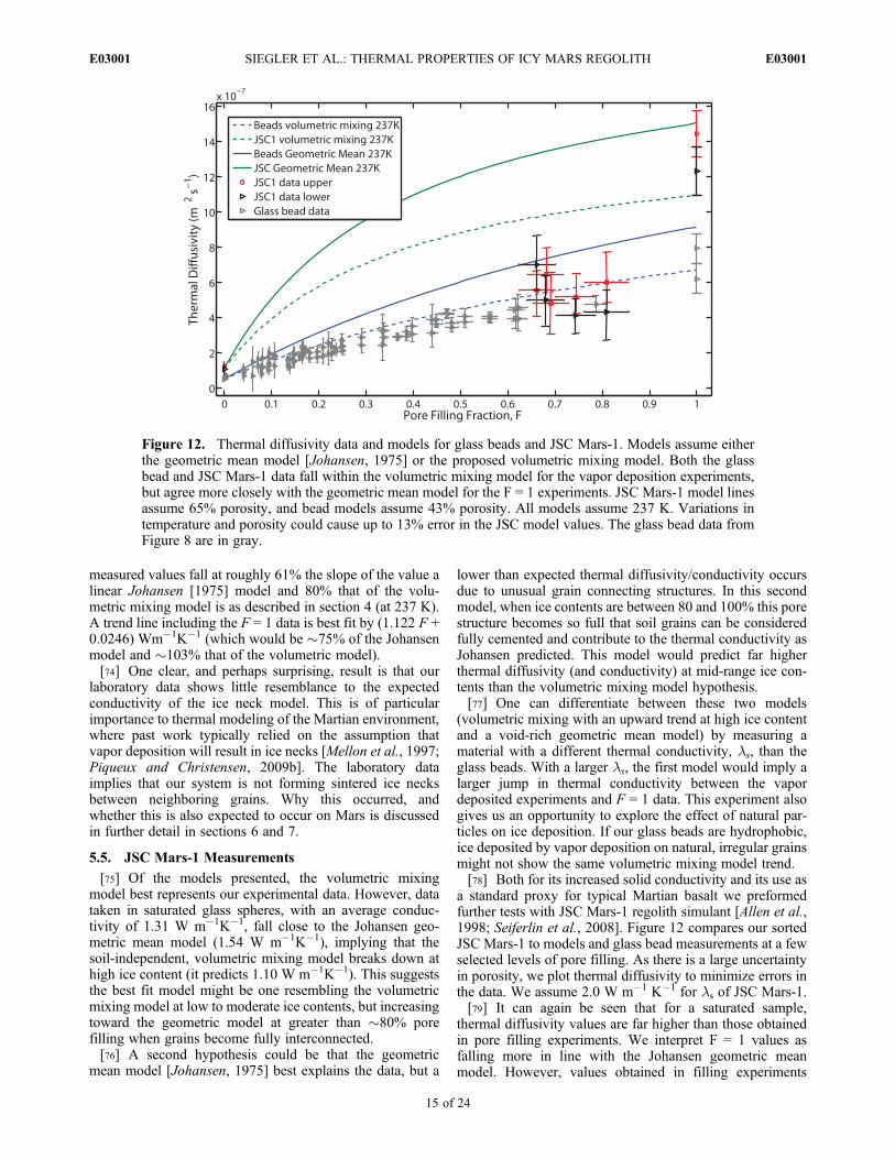
a standard proxy for typical Martian basalt we preformedfurther tests with JSC Mars-1 regolith simulant [Allen et al.,1998; Seiferlin et al., 2008]. Figure 12 compares our sortedJSC Mars-1 to models and glass bead measurements at a fewselected levels of pore filling. As there is a large uncertaintyin porosity, we plot thermal diffusivity to minimize errors inthe data. We assume 2.0 W m�1 K�1 for ls of JSC Mars-1.[79] It can again be seen that for a saturated sample,

thermal diffusivity values are far higher than those obtainedin pore filling experiments. We interpret F = 1 values asfalling more in line with the Johansen geometric meanmodel. However, values obtained in filling experiments

Figure 12. Thermal diffusivity data and models for glass beads and JSC Mars-1. Models assume eitherthe geometric mean model [Johansen, 1975] or the proposed volumetric mixing model. Both the glassbead and JSC Mars-1 data fall within the volumetric mixing model for the vapor deposition experiments,but agree more closely with the geometric mean model for the F = 1 experiments. JSC Mars-1 model linesassume 65% porosity, and bead models assume 43% porosity. All models assume 237 K. Variations intemperature and porosity could cause up to 13% error in the JSC model values. The glass bead data fromFigure 8 are in gray.


15 of 24

(269 h results are plotted here) show that all vapor-filledsamples fall closer to, and even lower than, those expectedby the volumetric mixing model. We suggest that the volu-metric model best explains the vapor deposition data asproposed by the first hypothesis above. In this model, thenon-ice soil matrix has little to no effect on the bulk thermalconductivity at lower ice contents (below the maximumfilling fractions achieved in the filling experiments), but alarge rise in thermal conductivity occurs between 80% and100% volumetric pore-filling. The difference between thevapor filled and F = 1 data may be a result of bubbles andvoids trapped within the ice that may both inhibit heattransfer and preserve anisotropic heat flow as discussedin section 6.

6. Microstructure of Vapor Deposited Ice

6.1. Microstructure: Low Ice Content

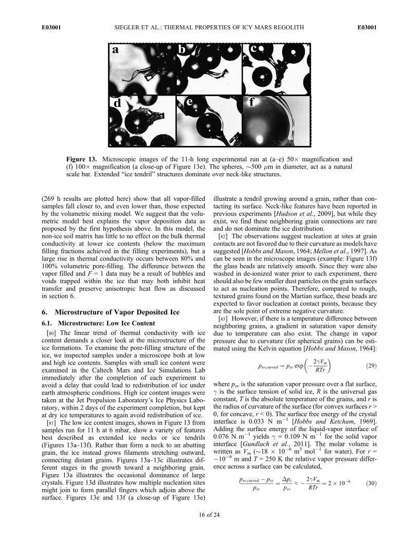
[80] The linear trend of thermal conductivity with icecontent demands a closer look at the microstructure of theice formations. To examine the pore-filling structure of theice, we inspected samples under a microscope both at lowand high ice contents. Samples with small ice content wereexamined in the Caltech Mars and Ice Simulations Labimmediately after the completion of each experiment toavoid a delay that could lead to redistribution of ice underearth atmospheric conditions. High ice content images weretaken at the Jet Propulsion Laboratory’s Ice Physics Labo-ratory, within 2 days of the experiment completion, but keptat dry ice temperatures to again avoid redistribution of ice.[81] The low ice content images, shown in Figure 13 from

samples run for 11 h at 6 mbar, show a variety of featuresbest described as extended ice necks or ice tendrils(Figures 13a–13f). Rather than form a neck to an abuttinggrain, the ice instead grows filaments stretching outward,connecting distant grains. Figures 13a–13c illustrates dif-ferent stages in the growth toward a neighboring grain.Figure 13a illustrates the occasional dominance of largecrystals. Figure 13d illustrates how multiple nucleation sitesmight join to form parallel fingers which adjoin above thesurface. Figures 13e and 13f (a close-up of Figure 13e)

illustrate a tendril growing around a grain, rather than con-tacting its surface. Neck-like features have been reported inprevious experiments [Hudson et al., 2009], but while theyexist, we find these neighboring grain connections are rareand do not dominate the ice distribution.[82] The observations suggest nucleation at sites at grain

contacts are not favored due to their curvature as models havesuggested [Hobbs and Mason, 1964;Mellon et al., 1997]. Ascan be seen in the microscope images (example: Figure 13f)the glass beads are relatively smooth. Since they were alsowashed in de-ionized water prior to each experiment, thereshould also be few smaller dust particles on the grain surfacesto act as nucleation points. Therefore, compared to rough,textured grains found on the Martian surface, these beads areexpected to favor nucleation at contact points, because theyare the sole point of extreme negative curvature.[83] However, if there is a temperature difference between

neighboring grains, a gradient in saturation vapor densitydue to temperature can also exist. The change in vaporpressure due to curvature (for spherical grains) can be esti-mated using the Kelvin equation [Hobbs and Mason, 1964]:

psv;curved ¼ psv exp � 2gVm

RTr

� �ð29Þ

where psv is the saturation vapor pressure over a flat surface,g is the surface tension of solid ice, R is the universal gasconstant, T is the absolute temperature of the grains, and r isthe radius of curvature of the surface (for convex surfaces r >0, for concave, r < 0). The surface free energy of the crystalinterface is 0.033 N m�1 [Hobbs and Ketcham, 1969].Adding the surface energy of the liquid-vapor interface of0.076 N m�1 yields g = 0.109 N m�1 for the solid vaporinterface [Gundlach et al., 2011]. The molar volume iswritten as Vm (�18 � 10�6 m3 mol�1 for water). For r =�10�6 m and T = 250 K the relative vapor pressure differ-ence across a surface can be calculated,

psv;curved � psvpsv

¼ Dpcpsv

≈ � 2gVm

RTr¼ 2� 10�6 ð30Þ

Figure 13. Microscopic images of the 11-h long experimental run at (a–e) 50� magnification and(f) 100� magnification (a close-up of Figure 13e). The spheres, �500 mm in diameter, act as a naturalscale bar. Extended “ice tendril” structures dominate over neck-like structures.


16 of 24

Meanwhile, the local difference in partial pressure caused bythe temperature difference across a grain (diameter d) can beapproximated as

DpT ¼ ∂psv∂T

gd; ð31Þ

where psv is the saturation vapor pressure

psvðTÞ ¼ pt exp �QLH

R

1

T� 1

Tt

� �� ; ð32Þ

with pt (611.7 Pa) and Tt (273.16 K) are the triple pointpressure and temperature of H2O, and QLH is the latent heatof sublimation (QLH/R ≈ 6130 K). In our experimental setup,with a nominal temperature gradient g = 900 K m�1,assuming the average T of 237 K,

DpTpsv

¼ QLH

RT2gd ≈ 0:049: ð33Þ

Thus, for our assumed neck radius and temperature gradientthe temperature effect exceeds the curvature effect by morethan four orders of magnitude (comparing equations (30)and (33)).[84] The radius of curvature at the contact can be better

approximated by examining the grain roughness. Roughgrains do not simply touch at a point [Bahrami et al., 2006]and the separation distance at the contact point of neigh-boring grains can be estimated to scale as twice the surfaceroughness [Slavin et al., 2002]. Using a MicroXAM opticalprofiler (ADE Phase Shift Co.) at the UCLA Ion ProbeFacility, the average surface of a fresh glass bead was foundto have surface imperfections on the order of 2 to 3 mm. Thatleads to an estimated contact point separation, and thereforeradius of curvature of the grain contact of �0.5 mm.[85] The radius of curvature will increase with ice content

if ice were to form at the contact point. Therefore, ice formingat a grain contact will decrease the curvature driving forcesand inhibit further growth at the contact. For random packingan average of 6 grain contacts occur around each void [Slavinet al., 2002], half of which contribute to ice volume within avoid, which results in 3 entire neck volumes per unit cell.Assuming a void volume of Vvoid ≈ (4/3p�o rgrain

3 )/(1 � �o)[Slavin et al., 2002] and Vneck = p2x4/(4rgrain) as the volumeof a single neck with neck radius of curvature rneck = x2/(2rgrain) [Hobbs and Mason, 1964], results in the relation

rneck ≈2rgrain3

ffiffiffiffiffiffiffiffiffiffiffiffiffiffiffiffiffiffiffiF�o

pð1� �oÞ

s; ð34Þ

which for 500 mm grains and 43% porosity, �o, even a smallF = 0.015 already results in rneck = 10 mm, decreasing thedriving force discussed in equation (30) by an order ofmagnitude.[86] If instead the temperature gradient is the driving force

behind the observed structures, then when Dpc > DpT, asdefined in equations (30) and (33), ice necks should be thedominant formation of inter-granular ice. In our experiment,which uses 500 mm spheres with an assumed 0.5 mm radiusof cuvature due to grain roughness, temperatures between�200 and 268 K fall above the transition for gradients

higher than about 10�2 K m�1. Though local, grain-to-graingradients have not been measured in our set-up, taking thelarge scale gradients to be representative of those at the grainscale results in 900 K m�1, five orders of magnitude higher.Therefore, sintered ice necks are not expected to form in ourexperiment.[87] The vapor density gradient is dependent both on the

local temperature gradient and the absolute temperature.Therefore, for a given gradient at various absolute tempera-tures, one might expect a transition between curvaturedominated (neck-like) and temperature dominated (tendril-like) inter-grain ice formation. Despite having average tem-peratures gradients much lower than this experimental setup,it is unlikely that surface conditions on Mars, the Moon orother potentially icy bodies cross this boundary. Even thegeothermal gradient of the Moon, which would serve as alower limit for the time averaged gradient, was measured tobe 0.79 K m�1 or higher [Langseth et al., 1976]. Further-more, at lower temperature gradients, water molecules willnot move efficiently by vapor diffusion. Lower absolutetemperatures may cause amorphous, rather than crystalline,ice to dominate [Schmitt et al., 1989].[88] In light of these considerations, the ice filling struc-

tures observed in our experiment can be explained by localtemperature conditions. Even the near-perfect grains in thisexperiment have small surface defects. Water vapor enteringa void would be most stable at a small defect on the coldestavailable grain, where there is both a thermal and Gibbs free-energy advantage due to a possible surface defect withinward curvature. Conversely, the grain contact wouldpresent a point of inward curvature with one cool and onewarm face. In addition, the high heat flux through the graincontact will cause the contact point in the cold grain to besubstantially warmer than the rest of the grain [Piqueux andChristensen, 2009a], potentially driving molecules awayfrom, rather than toward, this point. The contact is thecoolest point on the warm grain, but is warmer than anypoint on the cold grain. This would inhibit ice growth at thegrain contact, favoring initial ice growth at any otherimperfection on the cold bead’s surface.[89] Once ice begins to grow at a cold defect it may be a

preferential site for further ice growth, as it maximizes thesurface area exposed to the saturated gas. In a saturatedenvironment (as we have below the ice table) this point willcontinue to gain ice, growing outward from the surface. Ifthere is a nearby, but not directly connected, grain across thepore that is also cold, there will be a lower vapor densitynear the surface of this grain (attracting water vapor fromareas of higher density), aiding in directing the growth of theice tendril in that direction (as in Figures 13e and 13f). Thisgrowth scenario would explain the connection between rel-atively distant neighbors seen in the microscope images.Figures 13e and 13f illustrate a tendril growing around agrain which, in this scenario, would have been slightlywarmer and unfavorable for surface ice growth.[90] It is also possible that the grain surface is hydropho-

bic relative to JSC Mars-1 and other natural materials,repelling water molecules that landed there. However, as thehydrophobic and hydrophilic nature of a grain will onlyaffect surface tension, it can be expected that any such sur-face effect will be on the same order as that from graincurvature (i.e., equation (30)), and therefore be relatively


17 of 24

unimportant in determining ice formation. Regardless ofthe cause, molecules being repelled from a grain (i.e.,Figure 13f) and neighboring grain surfaces may form a laneof high vapor concentration, along which tendrils preferen-tially grow. The feature in Figure 13f could be explained bytwo independent tendrils growing along such an avenue anduniting mid-way.

6.2. Microstructure: Medium Ice Contentand Anisotropic Ice Growth

[91] The small scale structures, which appear to be con-trolled by local thermal gradients, will adjoin to form largerice formations. The net thermal gradient orients individualtendrils which can join to create long filamentous structures.At low ice content (<�20% pore filling fraction in ourexperiment) ice grows primarily along the thermal gradient.At higher ice contents, ice growth proceeds, but the ratio ofkx to kz remains relatively constant (Figure 9).[92] Figure 14 illustrates a sample from the upper 4 cm of

a 24 h long experiment (�15–20% pore filling fraction).Figure 14a shows a clear fabric of ice connected glass beadswhich forms a lineation in the vertical (z) direction (thesample surface is to the right in these images). Figures 14band 14c illustrate the filaments of the ice/grain fabric atvarious stages of dissection. Figures 14d and 14e aremicroscopic images of the dissected filaments seen in 14cand show that these filaments are constructed of multipleice tendrils, like those examined in Figure 13. Figures 14dand 14e are oriented in the same manner as Figure 14a,with the sample surface to the right.[93] We interpret these structures to be responsible for the

anisotropic thermal diffusivity observed in Figures 9 and 10.Ice growth, initially controlled by the forces described byequation (33), will preferentially link a grain to its coldest

neighbor. Due to the underlying thermal gradient in oursample, that next coldest grain is likely to be lower in thesample. As can be seen in Figures 14d and 14e, the coldgrain is often several grains away, and ice often takes tor-tuous pathways to reach the cold surface. The net results ofthis growth are heat pathways in the z-direction, as impliedby the single needle conductivity and dual needle hetcapacity measurements. The heat capacity measurementssuggest that this anisotropic growth stabilizes at about 20%pore filling fraction. At this point, the rate of anisotropicgrowth slows, maintaining a ratio of kx/kz of about 0.25.However, as seen in Figures 9 and 10, this underlyinganisotropic structure continues to dominate thermal proper-ties until very high ice contents (at least 80%). Our ice sat-urated (F = 1) experiments show no evidence of anisotropicthermal properties.

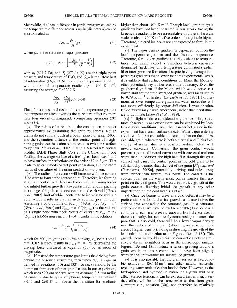
6.3. Microstructure: High Ice Content

[94] As ice growth continues, tendrils will further inter-twine, but, as hinted in the dual needle measurements, willretain an underlying anisotropic structure. Images at high icecontents can aid in interpreting what remnants of the initialpore filling structure control high ice content thermal prop-erties. The images in Figure 15 have been obtained undertransmitted illumination with an Olympus BX51 microscopeequipped with a LN2-cooled Linkam LTS 350 cryostage atthe Jet Propulsion Laboratory’s Ice Physics Laboratorywhich was pre-cooled to �30�C to avoid any melting of thesamples.[95] Figure 15 shows evidence of voids and bubbles

within ice resulting from an experimental run after 570 h.The samples in these images were found to have roughly75–80% pore filling fraction, F, by a gravimetric measure.

Figure 14. Photographic and microscopic evidence for preferential ice tendril growth in the z direction.These samples taken from a 24 hour long experiment, reveal anisotropic ice growth and are consistent withthe anisotropic thermal diffusivity observed with the dual needle measurements (as seen in Figures 9–11).(a–c) The large-scale fabric of the ice tendrils. (d and e) The ice linkages that form between individualgrains to create tendrils.


18 of 24

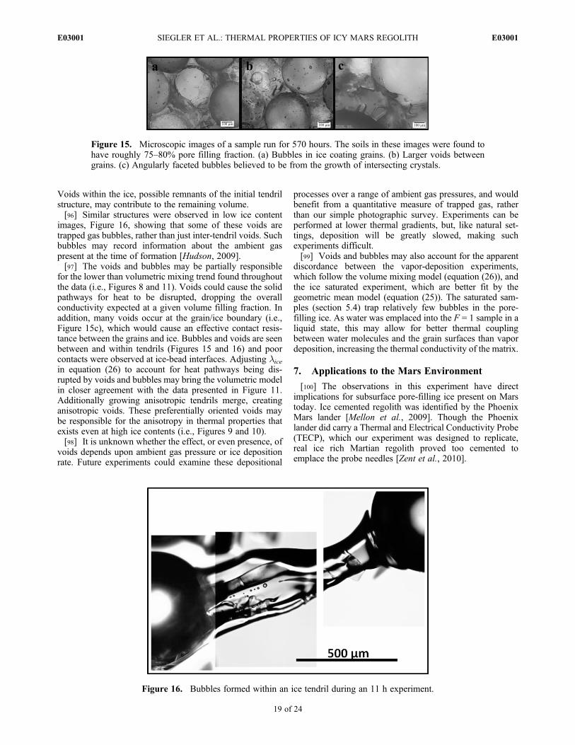
Voids within the ice, possible remnants of the initial tendrilstructure, may contribute to the remaining volume.[96] Similar structures were observed in low ice content

images, Figure 16, showing that some of these voids aretrapped gas bubbles, rather than just inter-tendril voids. Suchbubbles may record information about the ambient gaspresent at the time of formation [Hudson, 2009].[97] The voids and bubbles may be partially responsible

for the lower than volumetric mixing trend found throughoutthe data (i.e., Figures 8 and 11). Voids could cause the solidpathways for heat to be disrupted, dropping the overallconductivity expected at a given volume filling fraction. Inaddition, many voids occur at the grain/ice boundary (i.e.,Figure 15c), which would cause an effective contact resis-tance between the grains and ice. Bubbles and voids are seenbetween and within tendrils (Figures 15 and 16) and poorcontacts were observed at ice-bead interfaces. Adjusting licein equation (26) to account for heat pathways being dis-rupted by voids and bubbles may bring the volumetric modelin closer agreement with the data presented in Figure 11.Additionally growing anisotropic tendrils merge, creatinganisotropic voids. These preferentially oriented voids maybe responsible for the anisotropy in thermal properties thatexists even at high ice contents (i.e., Figures 9 and 10).[98] It is unknown whether the effect, or even presence, of

voids depends upon ambient gas pressure or ice depositionrate. Future experiments could examine these depositional

processes over a range of ambient gas pressures, and wouldbenefit from a quantitative measure of trapped gas, ratherthan our simple photographic survey. Experiments can beperformed at lower thermal gradients, but, like natural set-tings, deposition will be greatly slowed, making suchexperiments difficult.[99] Voids and bubbles may also account for the apparent

discordance between the vapor-deposition experiments,which follow the volume mixing model (equation (26)), andthe ice saturated experiment, which are better fit by thegeometric mean model (equation (25)). The saturated sam-ples (section 5.4) trap relatively few bubbles in the pore-filling ice. As water was emplaced into the F = 1 sample in aliquid state, this may allow for better thermal couplingbetween water molecules and the grain surfaces than vapordeposition, increasing the thermal conductivity of the matrix.

7. Applications to the Mars Environment

[100] The observations in this experiment have directimplications for subsurface pore-filling ice present on Marstoday. Ice cemented regolith was identified by the PhoenixMars lander [Mellon et al., 2009]. Though the Phoenixlander did carry a Thermal and Electrical Conductivity Probe(TECP), which our experiment was designed to replicate,real ice rich Martian regolith proved too cemented toemplace the probe needles [Zent et al., 2010].

Figure 15. Microscopic images of a sample run for 570 hours. The soils in these images were found tohave roughly 75–80% pore filling fraction. (a) Bubbles in ice coating grains. (b) Larger voids betweengrains. (c) Angularly faceted bubbles believed to be from the growth of intersecting crystals.

Figure 16. Bubbles formed within an ice tendril during an 11 h experiment.


19 of 24

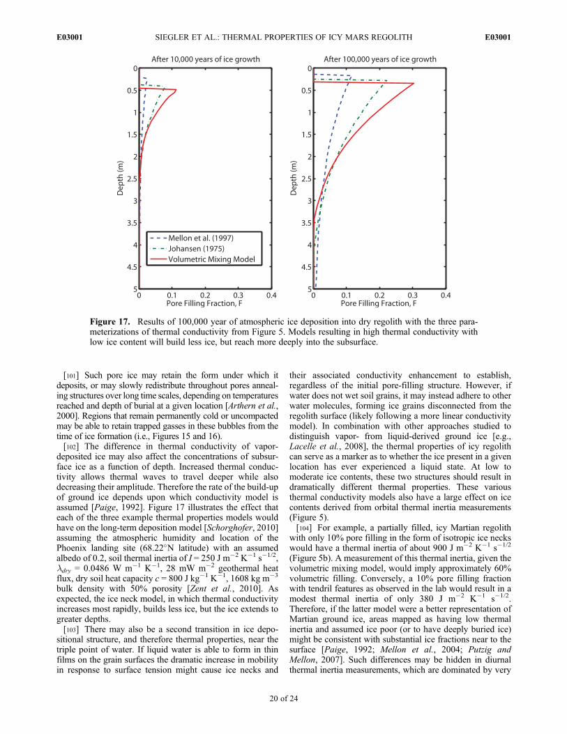
[101] Such pore ice may retain the form under which itdeposits, or may slowly redistribute throughout pores anneal-ing structures over long time scales, depending on temperaturesreached and depth of burial at a given location [Arthern et al.,2000]. Regions that remain permanently cold or uncompactedmay be able to retain trapped gasses in these bubbles from thetime of ice formation (i.e., Figures 15 and 16).[102] The difference in thermal conductivity of vapor-

deposited ice may also affect the concentrations of subsur-face ice as a function of depth. Increased thermal conduc-tivity allows thermal waves to travel deeper while alsodecreasing their amplitude. Therefore the rate of the build-upof ground ice depends upon which conductivity model isassumed [Paige, 1992]. Figure 17 illustrates the effect thateach of the three example thermal properties models wouldhave on the long-term deposition model [Schorghofer, 2010]assuming the atmospheric humidity and location of thePhoenix landing site (68.22�N latitude) with an assumedalbedo of 0.2, soil thermal inertia of I = 250 J m�2 K�1 s�1/2,ldry = 0.0486 W m�1 K�1, 28 mW m�2 geothermal heatflux, dry soil heat capacity c = 800 J kg�1 K�1, 1608 kg m�3

bulk density with 50% porosity [Zent et al., 2010]. Asexpected, the ice neck model, in which thermal conductivityincreases most rapidly, builds less ice, but the ice extends togreater depths.[103] There may also be a second transition in ice depo-

sitional structure, and therefore thermal properties, near thetriple point of water. If liquid water is able to form in thinfilms on the grain surfaces the dramatic increase in mobilityin response to surface tension might cause ice necks and

their associated conductivity enhancement to establish,regardless of the initial pore-filling structure. However, ifwater does not wet soil grains, it may instead adhere to otherwater molecules, forming ice grains disconnected from theregolith surface (likely following a more linear conductivitymodel). In combination with other approaches studied todistinguish vapor- from liquid-derived ground ice [e.g.,Lacelle et al., 2008], the thermal properties of icy regolithcan serve as a marker as to whether the ice present in a givenlocation has ever experienced a liquid state. At low tomoderate ice contents, these two structures should result indramatically different thermal properties. These variousthermal conductivity models also have a large effect on icecontents derived from orbital thermal inertia measurements(Figure 5).[104] For example, a partially filled, icy Martian regolith

with only 10% pore filling in the form of isotropic ice neckswould have a thermal inertia of about 900 J m�2 K�1 s�1/2

(Figure 5b). A measurement of this thermal inertia, given thevolumetric mixing model, would imply approximately 60%volumetric filling. Conversely, a 10% pore filling fractionwith tendril features as observed in the lab would result in amodest thermal inertia of only 380 J m�2 K�1 s�1/2.Therefore, if the latter model were a better representation ofMartian ground ice, areas mapped as having low thermalinertia and assumed ice poor (or to have deeply buried ice)might be consistent with substantial ice fractions near to thesurface [Paige, 1992; Mellon et al., 2004; Putzig andMellon, 2007]. Such differences may be hidden in diurnalthermal inertia measurements, which are dominated by very

Figure 17. Results of 100,000 year of atmospheric ice deposition into dry regolith with the three para-meterizations of thermal conductivity from Figure 5. Models resulting in high thermal conductivity withlow ice content will build less ice, but reach more deeply into the subsurface.


20 of 24

near surface material that tends to be ice free in depositionmodels (Figure 17), but may be prominent in more deeplypenetrating, seasonal temperature variations.

8. Conclusions

[105] Icy regolith was created in the laboratory by vapordeposition under Martian atmospheric pressure (6 mbar) andsub-freezing temperatures. We have measured the thermaldiffusivity with a multineedle probe and the heat capacitywith a calorimeter. For this purpose, we have extended theequations for inversion of single and dual needle probemeasurements to an anisotropic medium. The thermal con-ductivity of 500–600 mm sized glass beads and JSC Mars-1is best fit by a linear volumetric mixing model between iceand dry regolith.[106] For the glass beads, the quantitative results for ther-

mal conductivity are plotted in Figure 11 and given by

lz Fð Þ ¼ ½ð0:88� 0:06ÞF þ 7:5� 10�2� Wm�1K�1 ð35Þ

at T = 237 K for pore filling fractions between 0 and 0.75.This is essentially identical to volumetric mixing model,equation (26), except the thermal conductivity of ice isreduced to 80%. Equation (35) can be approximatelyrewritten as

lz F; Tð Þ ¼ ð0:80� 0:05Þ�0lice Tð ÞF þ ldry Tð Þ ð36Þ

within error of our measured ldry. At different ambientpressures, or under different thermal gradients, the prefactormay differ from 0.80 because thermal conductivity mayincrease as void and bubble volumes decrease. ldry alsodecreases with decreasing pressure (i.e., Figure 6). Thermaldiffusivity, kz, can be calculated as lz/rc as a function ofF and T.[107] A linear trend is also found in filling experiments

with JSC Mars-1 regolith simulant up to approximately 80%volumetric pore filling, as shown in Figure 12. At higherfilling fractions than those tested, thermal conductivity risestoward a saturated value and is consistent with the geometricmean of the components given by equations (24) and (25).[108] Photographic evidence reveals the formation of an

inter-grain structure of long ice tendrils (Figure 13). Thesetendrils differ from ice necks in that ice generally links agrain to a semi-distant neighbor. In the ice neck model, pore-filling ice initially forms links between grains in directcontact with each other. This tendril dominated structurecauses thermal conductivity to vary linearly with ice content,as in equation (36).[109] The absence of ice necks may be understood as an

effect of the large thermal gradients that can exist betweengrains at low atmospheric pressures. Under these conditions,vapor pressure changes caused by the local curvature of ameniscus are typically many orders of magnitude smallerthan those caused by temperature differences betweengrains, as described by equations (29)–(33). Therefore, evenunder very small local thermal gradients, tendrils should beexpected to form along the gradient, rather than isotropic iceneck structures. According to this theory, anisotropic icestructures are obtained even for smaller gradients than areexpected in nature.

[110] Our results further indicate that vapor-deposited icegrows anisotropically and preferentially along the directionof the vapor density gradient. Our experimental setup is notdesigned to accurately measure thermal diffusivity in thehorizontal direction, but an approximate value extractedfrom volumetric averages indicates the ratio of vertical tohorizontal thermal diffusivity reaches a factor of roughlyfour (Figures 9 and 10), and remains so to �80% pore fillingfractions. In addition, microscope images of undisturbedsamples whose orientation was maintained shows that thetendrils grow along the thermal gradient and form chains ofice-bonded grains (Figure 14).[111] Though the temperature gradients in our experiment

are larger than the time averaged temperature gradientsexperienced on Mars and the Moon, the arguments presentedhere for anisotropic ice growth and void formation shouldhold under natural conditions. Furthermore, ice will be mostmobile in these environments when instantaneous localthermal gradients, which may dominate ice mobility, arehigh. Depending on the pore-filling geometry, a given ther-mal inertia can correspond to substantially different ice con-tent (larger than a factor of two at a 10% pore filling fraction).[112] These experimental results may also have an impact

on assumed electrical and diffusive properties of planetaryregolith. Thermal and electrical conductivities are oftenintimately linked and considerations of pore-filling struc-tures may also affect interpretation of ice probed by radarmeasurements. Vapor diffusion models may also need toaccount for such structures. The tortuosity of an ice-filledmedium may be different if ice forms tendrils rather thannecks. Future experiments can attempt to measure thesequantities in light of ice formation processes as well as toprobe the effects of time varying temperatures and grain sizedistribution on ice filled thermal properties.

Appendix A: Error Analysis of Fit to Needle Data

[113] Many sources of error are accounted for in themeasured thermal properties in this experiment. Errorsshown for in derived thermal diffusivities arise from a non-linear fit and variation in supplied heat (q). Other errors,such as variation in needle spacing and edge effects areneglected, but small in comparison. Data from the lowestneedle touching the brass baseplate are not used.[114] Initially, the measured DT values (as illustrated in

Figure 4), are fit to equations (8) (for the cooling of theheated needle), (20) or (21) (for the neighboring needles) bya nonlinear least squares regression. The error in the non-linear fit also contain any uncertainty caused by inadequatetime or temperature resolution.[115] For single needle data (only data from the cooling

trend is presented in this paper) best fits for each variable l,tc, or d from equation (8) for a 300 s interval are calculatedas a fit coefficient, residual, and Jacobian. To find the rela-tive error in single needle thermal conductivity result, therelative error of a 95% confidence interval in the fit to l isadded in quadrature with the relative error in q′ (whichincludes uncertainties in current 0.109 � 0.006 A, voltage6.00 � 0.01 V, and length 0.060 � 0.001 m). This typicallygives a relative error of �6% a given measurement (verticalerror bars in Figures 7, 9, and 10). The effect of contact


21 of 24

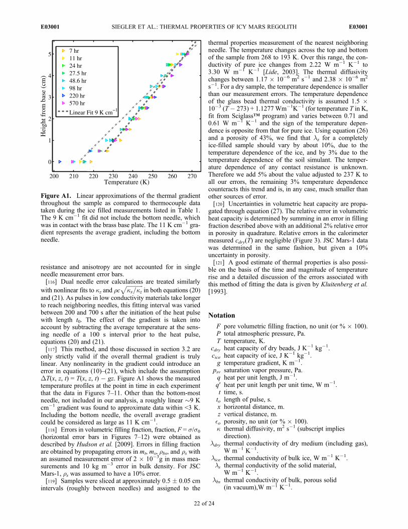
resistance and anisotropy are not accounted for in singleneedle measurement error bars.[116] Dual needle error calculations are treated similarly

with nonlinear fits to kz and rcffiffiffiffiffiffiffiffiffiffiffiffikx=kz

pin both equations (20)

and (21). As pulses in low conductivity materials take longerto reach neighboring needles, this fitting interval was variedbetween 200 and 700 s after the initiation of the heat pulsewith length t0. The effect of the gradient is taken intoaccount by subtracting the average temperature at the sens-ing needle of a 100 s interval prior to the heat pulse,equations (20) and (21).[117] This method, and those discussed in section 3.2 are

only strictly valid if the overall thermal gradient is trulylinear. Any nonlinearity in the gradient could introduce anerror in equations (10)–(21), which include the assumptionDT(x, z, t) = T(x, z, t) � gz. Figure A1 shows the measuredtemperature profiles at the point in time in each experimentthat the data in Figures 7–11. Other than the bottom-mostneedle, not included in our analysis, a roughly linear �9 Kcm�1 gradient was found to approximate data within <3 K.Including the bottom needle, the overall average gradientcould be considered as large as 11 K cm�1.[118] Errors in volumetric filling fraction, fraction, F = s/s0

(horizontal error bars in Figures 7–12) were obtained asdescribed by Hudson et al. [2009]. Errors in filling fractionare obtained by propagating errors in mt, ms, rbs, and rs withan assumed measurement error of 2 � 10�3g in mass mea-surements and 10 kg m�3 error in bulk density. For JSCMars-1, rs was assumed to have a 10% error.[119] Samples were sliced at approximately 0.5 � 0.05 cm

intervals (roughly between needles) and assigned to the

thermal properties measurement of the nearest neighboringneedle. The temperature changes across the top and bottomof the sample from 268 to 193 K. Over this range, the con-ductivity of pure ice changes from 2.22 W m�1 K�1 to3.30 W m�1 K�1 [Lide, 2003]. The thermal diffusivitychanges between 1.17 � 10�6 m2 s�1 and 2.38 � 10�6 m2

s�1. For a dry sample, the temperature dependence is smallerthan our measurement errors. The temperature dependenceof the glass bead thermal conductivity is assumed 1.5 �10�3 (T� 273) + 1.1277 Wm�1K�1 (for temperature T in K,fit from Sciglass™ program) and varies between 0.71 and0.61 W m�1 K�1 and the sign of the temperature depen-dence is opposite from that for pure ice. Using equation (26)and a porosity of 43%, we find that lz for a completelyice-filled sample should vary by about 10%, due to thetemperature dependence of the ice, and by 3% due to thetemperature dependence of the soil simulant. The temper-ature dependence of any contact resistance is unknown.Therefore we add 5% about the value adjusted to 237 K toall our errors, the remaining 3% temperature dependencecounteracts this trend and is, in any case, much smaller thanother sources of error.[120] Uncertainties in volumetric heat capacity are propa-

gated through equation (27). The relative error in volumetricheat capacity is determined by summing in an error in fillingfraction described above with an additional 2% relative errorin porosity in quadrature. Relative errors in the calorimetermeasured cdry(T) are negligible (Figure 3). JSC Mars-1 datawas determined in the same fashion, but given a 10%uncertainty in porosity.[121] A good estimate of thermal properties is also possi-

ble on the basis of the time and magnitude of temperaturerise and a detailed discussion of the errors associated withthis method of fitting the data is given by Kluitenberg et al.[1993].

Notation

F pore volumetric filling fraction, no unit (or % � 100).P total atmospheric pressure, Pa.T temperature, K.

cdry heat capacity of dry beads, J K�1 kg�1.cice heat capacity of ice, J K�1 kg�1.g temperature gradient, K m�1.

psv saturation vapor pressure, Pa.q heat per unit length, J m�1.q′ heat per unit length per unit time, W m�1.t time, s.to length of pulse, s.x horizontal distance, m.z vertical distance, m.�o porosity, no unit (or % � 100).k thermal diffusivity, m2 s�1 (subscript implies

direction).ldry thermal conductivity of dry medium (including gas),

W m�1 K�1.lice thermal conductivity of bulk ice, W m�1 K�1.ls thermal conductivity of the solid material,

W m�1 K�1.lbs thermal conductivity of bulk, porous solid

(in vacuum),W m�1 K�1.

Figure A1. Linear approximations of the thermal gradientthroughout the sample as compared to thermocouple datataken during the ice filled measurements listed in Table 1.The 9 K cm�1 fit did not include the bottom needle, whichwas in contact with the brass base plate. The 11 K cm�1 gra-dient represents the average gradient, including the bottomneedle.


22 of 24

rbulk bulk density of the porous medium, kg m�3.rice density of bulk ice, kg m�3.rs density of the solid material, kg m�3.

[122] Acknowledgments. We thank Julie Castillo, Doug Cobos,Michael Hecht, Gerard Kluitenberg, Kenneth Libbrecht, Michael Mellon,David Paige, Marsha Presley, Al Slavin, and Steven Wood for their usefuldiscussions and Axel Schmidt for aid in measuring grain surface roughness,Karen Wacker for the construction of and insightful discussion in designingour thermal properties probe, and Hermann Engelhardt, Liz Carey, andKenny Oslund for years of guidance and dedication in the lab. This workwas supported by the Mars Fundamental Research Program. Part of thiswork has been conducted at the Jet Propulsion Laboratory, California Insti-tute of Technology, under contract to NASA. Government sponsorshipacknowledged.

ReferencesAllen, C. C., R. V. Morris, D. J. Lindstrom, M. M. Lindstrom, and J. P.Lockwood (1998), JSC Mars-1: Martian regolith simulant, Lunar Planet.Sci., XXVIII, Abstract 1259.

Arthern, R. J., D. P. Winebrenner, and E. D. Waddington (2000), Densifi-cation of water ice deposits on the residual north polar cap of Mars, Icarus,144, 367–381, doi:10.1006/icar.1999.6308.

Bahrami, M., M. M. Yovanovich, and J. R. Culham (2006), Effective ther-mal conductivity of rough spherical packed beds, Int. J. Heat MassTransfer, 49, 3691–3701, doi:10.1016/j.ijheatmasstransfer.2006.02.021.

Bristow, K. L., R. D. White, and G. J. Kluitenberg (1994), Comparison ofsingle and dual probes for measuring soil thermal properties with tran-sient heating, Aust. J. Soil Res., 32, 447–464, doi:10.1071/SR9940447.

Campbell, G. S., K. Calissendorff, and J. H. Williams (1991), Probe formeasuring soil specific heat using a heat pulse method, Soil Sci. Soc.Am. J., 55, 291–293, doi:10.2136/sssaj1991.03615995005500010052x.

Carson, J. K., S. J. Lovatt, D. J. Tanner, and A. C. Cleland (2005), Thermalconductivity bounds for isotropic, porous materials, Int. J. Heat MassTransfer, 48, 2150–2158, doi:10.1016/j.ijheatmasstransfer.2004.12.032.

Christensen, P. R., and H. J. Moore (1992), The Martian surface layer,in Mars, edited by H. H. Kieffer et al., pp. 686–729, Univ. of Ariz. Press,Tucson.

Cremers, C. J. (1971), Thermal conductivity cell for small powdered sam-ples, Rev. Sci. Instrum., 42, 1694–1696, doi:10.1063/1.1684970.

Cremers, C. J., and H. S. Hsia (1974), Thermal conductivity of Apollo 16lunar fines, Proc. Lunar Sci. Conf., 5th, 2703–2708.

Cull, J. P. (1978), Thermal contact resistance in transient conductivity mea-surements, J. Phys. E Sci. Instrum., 11, 323–326, doi:10.1088/0022-3735/11/4/014.

Cuzzi, J. N. (1972), The subsurface nature of Mercury and Mars from ther-mal microwave emission, Ph.D. thesis, Calif. Inst. of Technol., Pasadena,Calif.

De Vries, D. A. (1952), A nonstationary method for determining thermalconductivity of soil in situ, Soil Sci., 73, 83–90, doi:10.1097/00010694-195202000-00001.

Dul’nev, G. N. and Sigalova Z. V. (1967), Effective thermal conductivity ofgranular materials, J. Eng. Phys. Thermophys., 13, 670–685.

Farouki, O. T. (1981), Thermal properties of soils in cold regions, Cold Reg.Sci. Technol., 5, 67–75.

Fountain, J. A., and E. A. West (1970), Thermal conductivity of particulatebasalt as a function of density in simulated lunar and Martian environ-ments, J. Geophys. Res., 75, 4063–4069, doi:10.1029/JB075i020p04063.

Gavriliev, I. (2008), Thermal conductivity of segregated ground ice, Perma-frost Periglacial Proc., 19, 333–340, doi:10.1002/ppp.628.

Gundlach, B., S. Kilias, E. Beitz, and J. Blum (2011), Micrometer-sized iceparticles for planetary-science experiments I. Preparation, critical rollingfriction force, and specific surface energy, Icarus, 214, 717–723,doi:10.1016/j.icarus.2011.05.005.

Hardy, B. (1998), ITS-90 formulations for vapor pressure, frostpoint, tem-perature dewpoint temperature, and enhancement factors in the range�100 to +100�C, in Proceedings of the Third International Symposiumon Humidity and Moisture, edited by B. Hardy, pp. 1–15, Natl. Phys.Lab., London.

Hobbs, P. V. (1974), Ice Physics, Oxford Univ. Press, New York.Hobbs, P. V., and W. M. Ketcham (1969), The planar growth of ice from thepure melt, in Physics of Ice: Proceedings of the International Symposiumon Physics of Ice, edited by N. Riehl, B. Bullemer, and H. Engelhardt,pp. 95–112, Plenum Press, New York.

Hobbs, P. V., and B. J. Mason (1964), The sintering and adhesion of ice,Philos. Mag., 9(98), 181–197, doi:10.1080/14786436408229184.

Hudson, T. L. (2009), Growth, diffusion, and loss of subsurface ice onMars: Experiments and models, Ph.D. thesis, Calif. Inst. of Technol.,Pasadena, Calif.

Hudson, T. L., O. Aharonson, and N. Schorghofer (2009), Laboratoryexperiments and models of diffusive emplacement of ground ice on Mars,J. Geophys. Res., 114, E01002, doi:10.1029/2008JE003149.

Jakosky, B. M. (1986), On the properties of Martian fines, Icarus, 66,117–124, doi:10.1016/0019-1035(86)90011-4.

Johansen, O. (1975), Thermal conductivity of soils, Ph.D. thesis, Univ. ofTrondheim, Trondheim, Norway.

Kersten, M. S. (1949), Laboratory research for the determination of the ther-mal properties of soils, Bull. 28, final report, Univ. of Minn. Eng. Exp.Sta., U.S. Army Corps of Eng., Minneapolis, Minn.

Kluitenberg, G. J., J. M. Ham, and K. L. Bristow (1993), Error analysis ofthe heat pulse method for measuring soil volumetric heat capacity, Soil Sci.Soc. Am. J., 57, 1444–1451, doi:10.2136/sssaj1993.03615995005700060008x.

Kossacki, K. J., N. I. Komle, G. Kargl, and G. Steiner (1994), The influenceof grain sintering on the thermal conductivity of porous ice, Planet. SpaceSci., 42, 383–389, doi:10.1016/0032-0633(94)90127-9.

Lacelle, D., D. Fisher, I. D. Clark, and A. Berinstain (2008), Distinguishingbetween vapor- and liquid-formed ground ice in the northern Martian rego-lith and potential for biosignatures preserved in ice bodies, Icarus, 197(2),458–469, doi:10.1016/j.icarus.2008.05.017.

Lachenbruch, A. H., J. H. Sass, B. V. Mashall, and T. H. Moses Jr. (1982),Permafrost, heat flow, and the geothermal regime at Prudhoe Bay, Alaska,J. Geophys. Res., 87, 9301–9316, doi:10.1029/JB087iB11p09301.

Langseth, M. G., S. J. Keihm, and K. Peters (1976), Revised lunar heat-flowvalues, Proc. Lunar Sci. Conf., 7th, 3143–3171.

Lide, D. R. (2003), CRC Handbook of Chemistry and Physics, 84th ed.,CRC Press, Boca Raton, Fla.

Mellon, M. T., and B. M. Jakosky (1993), Geographic variations in the thermaland diffusive stability of ground ice on Mars, J. Geophys. Res., 98(E2),3345–3364, doi:10.1029/92JE02355.

Mellon, M. T., B. M. Jakosky, and S. E. Postawko (1997), The persistence ofequatorial ground ice on Mars, J. Geophys. Res., 102(E8), 19,357–19,369,doi:10.1029/97JE01346.

Mellon, M. T., W. C. Feldman, and T. H. Prettyman (2004), The presenceand stability of ground ice in the southern hemisphere of Mars, Icarus,169, 324–340, doi:10.1016/j.icarus.2003.10.022.

Mellon, M. T., et al. (2009), Ground ice at the Phoenix landing site: Stabilitystate and origin, J. Geophys. Res., 114, E00E07, doi:10.1029/2009JE003417.

Mickley, A. S. (1951), The thermal conductivity of moist soil, Trans. Am.Inst. Electr. Eng., 70(2), 1789–1797.

Paige, D. (1992), The thermal stability of near-surface ground ice on Mars,Nature, 356(6364), 43–45, doi:10.1038/356043a0.

Piqueux, S., and P. R. Christensen (2009a), A model of thermal conductiv-ity for planetary soils: 1. Theory for unconsolidated soils, J. Geophys.Res., 114, E09005, doi:10.1029/2008JE003308.

Piqueux, S., and P. R. Christensen (2009b), A model of thermal conductiv-ity for planetary soils: 2. Theory for cemented soils, J. Geophys. Res.,114, E09006, doi:10.1029/2008JE003309.

Presley, M. A., and P. R. Christensen (1997a), Thermal conductivity mea-surements of particulate materials: 1. A review, J. Geophys. Res., 102(E3),6535–6549, doi:10.1029/96JE03302.

Presley, M. A., and P. R. Christensen (1997b), Thermal conductivity mea-surements of particulate materials: 2. Results, J. Geophys. Res., 102(E3),6551–6566, doi:10.1029/96JE03303.

Presley, M. A., and P. R. Christensen (2010), Thermal conductivity mea-surements of particulate materials: 5. Effect of bulk density and particleshape, J. Geophys. Res., 115, E07004, doi:10.1029/2009JE003483.

Presley, M. A., and R. A. Craddock (2006), Thermal conductivity measure-ments of particulate materials: 3. Natural samples and mixtures of particlesizes, J. Geophys. Res., 111, E09013, doi:10.1029/2006JE002706.

Putkonen, J. (2003), Determination of frozen soil thermal properties byheated needle probe, Permafrost Periglacial Proc., 14, 343–347, doi:10.1002/ppp.465.

Putzig, N. E., and M. T. Mellon (2007), Apparent thermal inertia and thesurface heterogeneity ofMars, Icarus, 191, 68–94, doi:10.1016/j.icarus.2007.05.013.

Sass, J. H., A. H. Lachenbruch, and R. J. Munroe (1971), Thermal conduc-tivity of rocks from measurements on fragments and its application toheat-flow determinations, J. Geophys. Res., 76, 3391–3401, doi:10.1029/JB076i014p03391.

Schmitt, B., S. Espinasse, R. J. A. Grim, J. M. Greenberg, and J. Klinger(1989), Laboratory studies of cometary ice analogues, Eur. Space AgencySpec. Publ., ESA SP-302, 65–69.

Schorghofer, N. (2010), Fast numerical method for growth and retreat ofsubsurface ice on Mars, Icarus, 208, 598–607, doi:10.1016/j.icarus.2010.03.022.


23 of 24

Schorghofer, N., and O. Aharonson (2005), Stability and exchange of sub-surface ice on Mars, J. Geophys. Res., 110, E05003, doi:10.1029/2004JE002350.

Schotte, W. (1960), Thermal conductivity of packed beds, Trans. Inst.Chem. Eng., 6, 63–67.

Seiferlin, K., P. Ehrenfreund, J. Garry, K. Gunderson, E. Hütter, G. Kargl,A. Maturilli, and J. P. Merrisone (2008), Simulating Martian regolith inthe laboratory, Planet. Space Sci., 56, 2009–2025, doi:10.1016/j.pss.2008.09.017.

Slavin, A. J., V. Arcas, C. A. Greenhalgh, E. R. Irvine, and D. B. Marshall(2002), Theoretical model for the thermal conductivity of a packed bed ofsolid spheroids in the presence of a static gas, with no adjustable parametersexcept at low pressure and temperature, Int. J. Heat Mass Transfer, 45,4151–4161, doi:10.1016/S0017-9310(02)00117-5.

Smoluchowski, M. (1910), Sur la conductibilité calorifique des corps pul-verizes, Bull. Acad. Sci. Cracovie, Ser. A, 5, 129–153.

Tsotsas, E., and H. Martin (1987), Thermal conductivity of packed beds:A review, Chem. Eng. Process., 22, 19–37, doi:10.1016/0255-2701(87)80025-9.

Vasavada, A. R., D. A. Paige, and S. E. Wood (1999), Near-surface tem-peratures on Mercury and the Moon and the stability of polar ice deposits,Icarus, 141, 179–193, doi:10.1006/icar.1999.6175.

Watson, K. (1964), I. The thermal conductivity measurements of selectedsilicate powders in vacuum from 150�–350�K, II. An interpretation ofthe Moon’s eclipse and lunation cooling as observed through the Earth’sAtmosphere from 8–14 microns, Ph.D. thesis, 186 pp., Div. of Geol. andPlanet. Sci., Calif. Inst. of Technol., Pasadena, Calif.

Wechsler, A. E., and P. E. Glaser (1965), Pressure effects on postulatedlunar materials, Icarus, 4, 335–352, doi:10.1016/0019-1035(65)90038-2.

Wechsler, A. E., P. E. Glaser, and J. A. Fountain (1972), Thermal propertiesof granulated materials, in Thermal Characteristics of the Moon, editedby J. W. Lucas, pp. 215–241, MIT Press, Cambridge, Mass.

Winter, D. F., and J. M. Saari (1969), A particulate thermophysical modelof the lunar soil, Astrophys. J., 156, 1135–1151, doi:10.1086/150041.

Wood, S. E. (2011), A general analytic model for the thermal conductivityof loose, indurated, or icy planetary regolith, Proc. Lunar Planet. Sci.Conf., 42nd, 2795.

Zent, A. P. (2008), A historical search for habitable ice at the Phoenix land-ing site, Icarus, 196(2), 385–408, doi:10.1016/j.icarus.2007.12.028.

Zent, A. P., M. H. Hecht, D. R. Cobos, S. E. Wood, T. L. Hudson, S. M.Milkovich, L. P. DeFlores, and M. T. Mellon (2010), Initial results fromthe thermal and electrical conductivity probe (TECP) on Phoenix, J. Geophys.Res., 115, E00E14, doi:10.1029/2009JE003420.

O. Aharonson, E. Carey, and S. Xu, Division of Geological and PlanetarySciences, California Institute of Technology, 1200 E. California Blvd.,Pasadena, CA 91125, USA.M. Choukroun and T. Hudson, Jet Propulsion Laboratory, California

Institute of Technology, 4800 Oak Grove Dr., Pasadena, CA 91109, USA.N. Schorghofer, Institute for Astronomy, University of Hawaii,

2680 Woodlawn Dr., Honolulu, HI 96822, USA.M. Siegler, Department of Earth and Space Sciences, University of

California, 595 Charles Young Dr. E., Box 951567, Los Angeles,CA 90095, USA. ([email protected])


24 of 24

Documents

Measurements of thermal properties of icy Mars regolith ...authors.library.caltech.edu/30059/1/Siegler2012p17729J_Geophys_Res... · Measurements of thermal properties of icy Mars