Embed Size (px)
Citation preview

Measures of congestionMeasures of congestionin container terminalsin container terminals
AIRO 2008 - Ischia10 September 2008
Matteo Salani – TRANSP-OR EPFLIlaria Vacca – TRANSP-OR EPFL
Arnaud Vandaele – Univ. of Louvain

OutlineOutline
Introduction and motivationIntroduction and motivation LiteratureLiterature ModelingModeling Congestion measuresCongestion measures OptimizationOptimization Preliminary resultsPreliminary results Future workFuture work

Container Terminals (CT)Container Terminals (CT)
Zone in a port to import/export/transship containers
Different areas in a terminal : berths, yard, gates
Container utilisation is the easiest way to transport goods
Optimization in CT:
•Berth allocation
•Quay Cranes scheduling
•Yard operations
Different types of vehicles to travel between the yard and the berth

MotivationMotivation
Along the quay, several boats with thousand containers are loaded/unloaded
These containers movement lead to an high traffic in the yard zone, where the most of slowdowns occur.
(Tactical) Terminal planners often optimize the distance (time) traveled by container carriers because it impacts directly on the performance indicators, disregarding:
- Congestion issues (operations slowdowns because of bottlenecks)
- Alternative solutions (symmetries)
considering deterministic data
Aim of this study:
- Model the terminal and develop mesures of congestion
- Evaluate the impacts of the optimization of such measures on the terminal

AssumptionsAssumptions
In the berth/yard allocation plans, we define a path as an OD pair:
- An origin (berth or block)
- A destination (berth or block)
- number of containers
We consider flows of containers over a working shift.
Decisions could be taken on:
- The berth allocation plan (boats and berths)
- The yard allocation plan (destination blocks)
- Demand splitting (for berth to block flows only)
Given Given a set of a set of pp paths, determine the destination blocks paths, determine the destination blocks

LiteratureLiterature
Layout:Kim et al. An optimal layout of container yards, OR Spectrum, 2007.
Congestion:Lee et al. An optimization model for storage yard management in transshipment hubs, OR Spectrum, 2006.
Beamon. System reliability and congestion in a material handling system, Computers Industrial Engineering, 1999.
R. Möhring, Routing in graphs, Plenary session - AIRO 2008
ModelingModeling
Basic element

ModelingModeling
(m x n) basic elements for a yard
Only Berth-to-Yard and Yard-to-Berth paths :
(xo,yo) – (xd,yd)
Coordinates system to indicate origin and destination of containers
yard
berth0,0 1,0 2,0 3,0
0,1
0,2
0,3
0,4
1,1
1,2
1,3
1,4
2,1
2,2
2,3
2,4

RoutingRouting
yard
berth0,0 1,0 2,0 3,0
0,1
0,2
0,3
0,4
1,1
1,2
1,3
1,4
2,1
2,2
2,3
2,4
Routing rules:
- Horizontal lanes are one way
- Vertical lanes are two way
Toward the block, closest left vertical lane, turn right.
Toward the quay, turn right at the first vertical lane.
Back to origin berth position.
Distance travelled, closed formula (Manhattan)
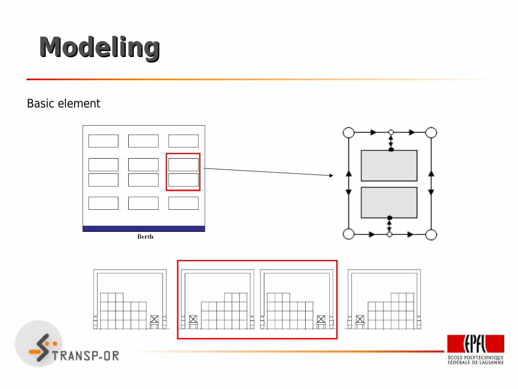
SymmetriesSymmetries
Minimize distance:
In a 2x2 yard with 2 paths, no capacity on blocks
Number of solutions with equal distance

MeasuresMeasures
Aim: Estimate the state/congestion of a yard when implementing a plan (using simple closed formulas) in order to identify secondary objectives.
We considered:
- Interference among blocks sharing the same lane
- Lane congestion
- Path interference

Block congestionBlock congestion
1
0ijb path j arrive in area iotherwise
# of containers in each area and best case :
we have s = 2n + n(m-1) areas
N i=∑j=1
p
b ij c jNx
=∑j=1
p
c j
r
Considered norm-1 and norm-2 with respect to the best over the worst case.
r = min(s, p)
Cb=D
Dmax
=∑j=1
p
N i−Nx2
r−1r
∑j=1
p
c j

Example with 2 normExample with 2 norm
Possible solutions = 1728

Edge congestionEdge congestion
It simply measure the average traffic over an edge
best traffic situation when flows are spread over the network
=maxk
f k0 =mink
f k0
Ce=−
∑j=1
n
c j
Ce=
n −∑j=1
p
c j
n−1 ∑j=1
p
c j
improved:

Path congestionPath congestion
Measure disturbances among paths.
Proximity matrix P (2p X 2p), symmetric, 0 on the diagonal, influenced by routing rules.
Worst case: all 1 matrix (except diagonal)
C p=1T P c
2p−1∑j=1
2p
c j
0,0 1,0 2,0 3,0
0,1
0,2
0,3
0,4
1,1
1,2
1,3
1,4
2,1
2,2
2,3
2,4

ExampleExample
Objective function : z=C bCeC p

ExampleExample
Objective function : z=C bCeC p
112,85120,4617354262144(2x2) – 6 paths
0,13
0,3473
0,4764
0,5068
0,3473
0,4764
MIN
4271
470
52
1831
282
46
Nb different values
108
350
116
21
30
10
Nb MIN
121,65248832(2x3) – 5 paths
7,2920736(2x3) – 4 paths
0,671728(2x3) – 3 paths
12,2332768(2x2) – 5 paths
1,44096(2x2) – 4 paths
0,2512(2x2) – 3 paths
CPU (s)Nb solutions

Algorithm: GRASPAlgorithm: GRASP
Greedy randomized adaptive search procedure
250,5121,650,13(2x3) – 5 paths
1503112,850,461(2x2) – 6 paths
15
0,1
0,1
0,5
0,2
0,1
CPU (s) (algorithm)
??
7,29
0,67
12,23
1,4
0,2
CPU (s)(enumeration)
1000
5
5
30
10
5
Nb iteration to reach optimum
0,1953(2x3) – 6 paths
0,3473(2x3) – 4 paths
0,4764(2x3) – 3 paths
0,5068(2x2) – 5 paths
0,3473(2x2) – 4 paths
0,4764(2x2) – 3 paths
MIN

more Testsmore Tests
More realistic instances
0,16460,16460,16460,16920,26(3x10) – 8
0,1624
0,1582
0,2763
0,267
0,195
0,13
0,3473
0,4764
in 10s
0,1609
0,1817
0,2763
0,267
0,195
0,13
0,3473
0,4764
in 20s
0,2670,2670,343(3x10) – 7
0,1950,1950,389(3x10) – 6
0,1663
0,1705
0,2763
0,13
0,3473
0,4764
in 5s
0,2276
0,1931
0,2763
0,13
0,3473
0,4764
in 1s
0,1389
0,1602
in 60s
0,3275(3x10) – 20
0,2446(3x10) – 15
0,304(3x10) – 9
0,13(3x10) – 5
0,3473(3x10) – 4
0,4764(3x10) – 3
in 0,1s

more Testsmore Tests
Other ongoing tests (3x10), 3 to 5 ships, up to 20 paths:
- Balanced/unbalanced repartition of loads among paths
- Balanced/unbalanced repartition of loads among ships
- Number of paths per ship (2 to 5)
Optimizing measures does not degradate too much the main objectives while helping in differentiate symmetric solutions

Conclusions and OutlookConclusions and Outlook
Simple closed formulas to evaluate congestion in container terminals
Useful to differentiate symmetric solutions with equal distance (or expected completion time)
TODO:
- Additional tests
- Multi-objective optimization problem, explore other than weighted sum
- Evaluate the effects with a CT simulator (queuing model)
- Improve the algorithm: study an exact approach, relax the assumptions, i.e. extend the set of possible decisions (berth allocation, demand splitting, working shifts)