Measures of problem uncertainty for scheduling with interval processing times

OR Spectrum (2013) 35:659–689DOI 10.1007/s00291-012-0306-3

REGULAR ARTICLE

Measures of problem uncertainty for schedulingwith interval processing times

Yuri N. Sotskov · Tsung-Chyan Lai ·Frank Werner

Published online: 19 September 2012© Springer-Verlag 2012

Abstract The paper deals with scheduling under uncertainty of the job processingtimes. The actual value of the processing time of a job becomes known only whenthe schedule is executed and may be equal to any value from the given interval. Wepropose an approach which consists of calculating measures of problem uncertaintyto choose an appropriate method for solving an uncertain scheduling problem. Thesemeasures are based on the concept of a minimal dominant set containing at least oneoptimal schedule for each realization of the job processing times. For minimizing thesum of weighted completion times of the n jobs to be processed on a single machine,it is shown that a minimal dominant set may be uniquely determined. We demonstratehow to use an uncertainty measure for selecting a method for finding an effectiveheuristic solution of the uncertain scheduling problem. The efficiency of the heuristicO(n log n)-algorithms is demonstrated on a set of randomly generated instances with100 ≤ n ≤ 5,000. A similar uncertainty measure may be applied to many otherscheduling problems with interval processing times.

Keywords Scheduling · Interval processing times · Uncertainty measure

Y. N. SotskovUnited Institute of Informatics Problems, National Academy of Sciences of Belarus,Surganova Street, 6, 220012 Minsk, Belaruse-mail: [email protected]

T.-C. LaiDepartment of Business Administration, National Taiwan University,2nd Management Building, 85, Sector 4, Roosevelt Road, 10672 Taipei, Taiwane-mail: [email protected]

F. Werner (B)Faculty of Mathematics, Otto-von-Guericke-University,Universitätsplatz 2, 39106 Magdeburg, Germanye-mail: [email protected]

123

660 Y. N. Sotskov et al.

1 Introduction

In real-life scheduling, the precise processing time may remain unknown until thecompletion of a job. Due to this reason, it may be impossible to implement a deter-ministic method (Pinedo 2002; Tanaev et al. 1994a,b) for constructing a really optimalschedule. In the OR literature, several methods for solving uncertain scheduling prob-lems have been developed (Kouvelis and Yu 1997; Pinedo 2002; Slowinski and Hapke1999; Sotskov et al. 2010). In a stochastic method (Ebben et al. 2005; Ivanescu etal. 2002; Pinedo 2002; Weiss 1976), it is assumed that the processing times are ran-dom variables with known probability distributions. If the processing times may bedefined as fuzzy numbers, a fuzzy logic is used for scheduling under fuzziness (Itohand Ishii 2005; Slowinski and Hapke 1999; Stanfield et al. 1996). If the processingtimes can be represented neither as random variables nor as fuzzy numbers, othermethods are needed for scheduling under uncertainty (Aytug et al. 2005; Kouvelisand Yu 1997; Sabuncuoglu and Goren 2009; Sotskov et al. 2010). A robust method(Daniels and Kouvelis 1995; Kasperski 2005; Kasperski and Zelinski 2008; Kouvelisand Yu 1997; Yang and Yu 2002) assumes that the decision-maker prefers a schedulehedging against the worst-case scenario. A stability method (Lai and Sotskov 1999;Sotskov et al. 2009; Sotskov and Lai 2012; Sotskov et al. 2010) combines a stabilityanalysis with a multi-stage decision framework.

Each of the above methods and other ones have a specific field for an efficientimplementation, a method suitable for one class of scheduling problems involvinguncertainty may fail for another class. A decision on selecting a method for solving aconcrete scheduling problem influences the quality of the schedule obtained and thetime needed for constructing an effective schedule.

In this paper, we propose using a measure of problem uncertainty for selectinga suitable method and for estimating the quality of a schedule which may be con-structed. In Sects. 2–7, we consider the single-machine problem of minimizing thesum of weighted completion times with a continuum of possible scenarios (Sect. 2).A survey of various methods is presented in Sects. 3.1–3.4. The uncertainty measures,which we suggest, are based on the cardinality of a minimal dominant set of job per-mutations (Sect. 3.4). For any feasible scenario, a minimal dominant set contains atleast one optimal permutation. In Sect. 4, we present a criterion for the largest car-dinality of a minimal dominant set. We show that a minimal dominant set may beuniquely determined (Sect. 5). Several examples are discussed in Sect. 6. The effi-ciency of the O(n log n)-algorithms is tested on randomly generated instances with100 ≤ n ≤ 5,000 (Sect. 7). In Sect. 8, we describe how to introduce a similar uncer-tainty measure for other more general scheduling problems. Section 9 is devoted toan application perspective in predictive–reactive scheduling. Concluding remarks aregiven in Sect. 10.

2 Problem description and preliminaries

In real-world scheduling, it is often necessary to manage a bottleneck machine.So, we first consider the following single-machine scheduling problem. A set of jobsJ = {J1, J2, . . . , Jn}, n ≥ 2, has to be processed on a single (bottleneck) machine, a

123

Measures of problem uncertainty for scheduling 661

weight wi > 0 being given for a job Ji ∈ J to reflect its importance. All the jobs J areready for processing from the start time t0 = 0 of the planning horizon. No preemptionis allowed while processing a job Ji ∈ J .

It is assumed that the processing time of a job Ji can take any real value pi ∈[pL

i , pUi ], only the bounds pL

i ≥ 0 and pUi ≥ pL

i of the segment [pLi , pU

i ] being givenbefore scheduling. The precise value pi remains unknown until the completion of jobJi . Such an assumption is realistic for most real-life scheduling problems since roughbounds pL

i and pUi may be given for a practical job Ji ∈ J : For a most uncertain job

Ji ∈ J , one can let pUi to be equal to the length of the planning horizon and pL

i = 0.

The set T of possible vectors p = (p1, p2, . . . , pn) of the job processing times iscalled the set of scenarios: T = {p | p ∈ Rn+, pL

i ≤ pi ≤ pUi , i ∈ {1, 2, . . . , n}}.

Note that there is a continuum of possible scenarios p ∈ T . Let S = {π1, π2, . . . , πn!}be the set of permutations πk = (Jk1 , Jk2 , . . . , Jkn ) of the jobs J .

If the scenario p ∈ T is fixed and the permutation πk ∈ S is chosen, then onecan calculate the completion time Ci = Ci (πk, p) of job Ji ∈ J in a semi-activeschedule (Ck1 , Ck2 , . . . , Ckn ) uniquely determined by the permutation πk . (A schedule(Ck1 , Ck2 , . . . , Ckn ) is called semi-active if no job Ji ∈ J can start earlier withoutdelaying the completion time of another job or altering the order πk for processingthe jobs J , see Pinedo 2002; Tanaev et al. 1994b.) Since the jobs J are ready forprocessing from time t0 = 0 and job preemptions are not allowed, one can calculate:Ck1 = pk1 , Cki = Cki−1 + pki−1 , i ∈ {2, 3, . . . , n}.

Using the three-field notation α|β|γ (Pinedo 2002), the problem consideredis denoted as 1|pL

i ≤ pi ≤ pUi | ∑ wi Ci , where the criterion γ = ∑

wi Ci

denotes the minimization of the sum of the weighted completion times: γ =∑Ji ∈J wi Ci = ∑

Ji ∈J wi Ci (πt , p) = minπk∈S{∑Ji ∈J wi Ci (πk, p)}, permutationπt = (Jt1 , Jt2 , . . . , Jtn ) ∈ S being optimal for the scenario p ∈ T .

As the scenario p ∈ T remains unknown until the completion of the jobs J ,

the values Ci , Ji ∈ J , cannot be calculated before the schedule realization. Thus,the problem 1|pL

i ≤ pi ≤ pUi | ∑wi Ci of finding an optimal permutation πt is not

correct (in general, it is not possible to find an exact solution to this problem since ascenario is not fixed). If a scenario p ∈ T is fixed, i.e., pL

i = pUi = pi ∈ [pi , pi ],

then problem 1|pLi ≤ pi ≤ pU

i | ∑wi Ci reduces to the problem 1||∑wi Ci , whichcan be solved in O(n log n) time (Smith 1956).

In what follows, the problem α|pLi ≤ pi ≤ pU

i |γ with the objective functionγ = f (C1, C2, . . . , Cn) is called uncertain in contrast to the problem α||γ which iscalled deterministic. Note that there is a principal difference between a deterministicproblem and its uncertain counterpart. While for solving any individual determinis-tic problem α||γ, one can apply the same method and an optimal schedule will beobtained (provided that an exact method will be applied), any two individual uncer-tain problems may need different methods to obtain a schedule which will be anex-post optimal or will provide objective function value close to an ex-post optimalone. (An ex-post optimal schedule is the best one that could been obtained if exactprocessing times of jobs J would have been available before scheduling.) First, theremay be no information available for implementing a particular method. Second, amethod may be not efficient or not effective for a specific instance of the problem

123


α|pLi ≤ pi ≤ pU

i |γ. Furthermore, while using a multi-stage decision framework, thesame instance may need a different method at different stages of the decision-making.

3 Literature review

While an optimal sequencing rule for the deterministic problem 1||∑ wi Ci has beenknown since 1956 (Smith 1956), its uncertain counterpart 1|pL

i ≤ pi ≤ pUi | ∑ wi Ci

continues to attract the researchers developing algorithms to solve it exactly (in somesense) or approximately, see Daniels and Kouvelis (1995), Kasperski (2005), Kasper-ski and Zelinski (2008), Pinedo (2002), Sotskov et al. (2009), Sotskov and Lai (2012),Weiss (1976) and Yang and Yu (2002) among others.

3.1 Robust method

For the problem α|pLi ≤ pi ≤ pU

i |γ, there usually does not exist a semi-active sched-ule (a job permutation for the problem 1|pL

i ≤ pi ≤ pUi |γ ) that remains optimal for all

scenarios from the set T . Due to this reason, an additional criterion is often introducedfor a problem α|pL

i ≤ pi ≤ pUi |γ. In particular, a robust schedule minimizing the

worst-case deviation from optimality was introduced in Daniels and Kouvelis (1995);Kouvelis and Yu (1997). Let γ t

p denote the optimal value of the non-decreasing objec-tive function γ = f (C1, C2, . . . , Cn) for the deterministic problem α||γ with thescenario p : γ t

p = minπk∈S γ kp = minπk∈S f (C1(πk, p), . . . , Cn(πk, p)). For the

permutation πk ∈ S and a scenario p ∈ T, the difference γ kp − γ t

p = r(πk, p)

is called the regret for πk, where permutation πt ∈ S is optimal. The valueZ(πk) = max{r(πk, p) | p ∈ T } is the worst-case absolute regret. The worst-caserelative regret is as follows: Z ′(πk) = max{ r(πk ,p)

γ tp

| p ∈ T }, γ tp �= 0. In Daniels

and Kouvelis (1995); Kasperski (2005); Kasperski and Zelinski (2008); Yang and Yu(2002), the problem 1|pL

i ≤ pi ≤ pUi | ∑ Ci has been considered (the job weights

are equal). For a specific scenario p j ∈ T, the deterministic problem 1||∑ Ci canbe solved using the shortest processing time (SPT) rule: Process the jobs J in non-decreasing order of their processing times p j

i , Ji ∈ J . While the deterministicproblem 1||∑ Ci is solvable in O(n log n) time, finding a permutation πt ∈ S ofminimizing either the worst-case absolute regret Z(πt ) or the relative regret Z ′(πk)

for the uncertain problem 1|pLi ≤ pi ≤ pU

i | ∑ Ci is NP-hard (Daniels and Kouvelis1995; Yang and Yu 2002). For the latter problem, a 2-approximation algorithm wasdeveloped to minimize the worst-case regret (Kasperski and Zelinski 2008) and sev-eral algorithms were tested (Daniels and Kouvelis 1995; Yang and Yu 2002). A fewspecial cases are known to be polynomially solvable for minimizing the worst-caseregret for the problems α|pL

i ≤ pi ≤ pUi |γ (Kasperski 2005).

3.2 Stochastic method

Part II of monograph (Pinedo 2002) is devoted to a stochastic method, allowing ascheduler to minimize the expectation E( f (C1, C2, . . . , Cn)) of the objective func-tion γ = f (C1, C2, . . . , Cn) for random processing times with known probability

123


distributions. An optimal schedule for problem 1|pLi ≤ pi ≤ pU

i |E(∑

wi Ci ) in theclass of non-preemptive static list policies (Pinedo 2002) (the jobs have to be orderedat time t0 = 0 according to a chosen priority rule) may be constructed by the weightedshortest expected processing time (WSEPT) rule: process the jobs in non-increasingorder of the ratios wi

E(pi ), where E(pi ) denotes the expected value of the random

processing time pi of the job Ji ∈ J (Pinedo 2002; Weiss 1976).In Tam et al. (2011), stochastic integer programming is used for airline crew schedul-

ing (it is necessary to find a set of pairings for a crew group to minimize the plannedcost of operating a schedule of aircraft flights). Taking into account the uncertainnature of aircraft delays, the authors of Tam et al. (2011) looked for a robust airlinecrew schedule which is less likely to be disrupted in the case of an aircraft delay. Theprobability of a flight delay was modeled by logistic regression and a flight delay timeby multi-variable regression.

3.3 Fuzzy method

If the processing times of the jobs J are given as fuzzy numbers, a fuzzy method isavailable for solving a scheduling problem under fuzziness. The book Slowinski andHapke (1999) is devoted to the fuzzy method used in a scheduling environment.

In Itoh and Ishii (2005), Tada et al. (1990), the authors propose a scheduling model,where the due dates for the jobs are random variables. The job processing times arescript, and one assigns satisfaction levels to the job completion times according tonon-increasing membership functions, their positions depending on the expected duedates, which are exponentially distributed.

3.4 Stability method

If no additional criterion is introduced (contrary to a robust method), there is noinformation on the probability distributions of the random processing times (contrary toa stochastic method) and there are no membership functions for non-script processingtimes (contrary to a fuzzy method), then a stability method (Sotskov et al. 2010) maybe used for a problem α|pL

i ≤ pi ≤ pUi |γ. This method combines a stability analysis,

a multi-stage decision framework and the solution concept of a minimal dominant set(Lai and Sotskov 1999; Sotskov et al. 2009, 2010).

Definition 1 A set of permutations S(T ) ⊆ S is a minimal dominant set for theproblem 1|pL

i ≤ pi ≤ pUi |γ, if for any scenario p ∈ T, the set S(T ) contains at least

one optimal permutation for the deterministic counterpart α||γ associated with thescenario p, this property being lost for any proper subset of set S(T ).

We recall some known results for the deterministic problem 1||∑wi Ci and for theuncertain problem 1|pL

i ≤ pi ≤ pUi | ∑ wi Ci .

123


Theorem 1 (Smith 1956) The permutation πk = (Jk1 , Jk2 , . . . , Jkn ) ∈ S is optimalfor the problem 1||∑ wi Ci if and only if the following inequalities hold:

wk1

pk1

≥ wk2

pk2

≥ · · · ≥ wkn

pkn

. (1)

Due to Theorem 1 (Smith 1956), the deterministic problem 1||∑ wi Ci can besolved by the weighted shortest processing time (WSPT) rule: process the jobs innon-increasing order of the weight-to-process ratios

wkipki

. For the uncertain problem

1|pLi ≤ pi ≤ pU

i | ∑ wi Ci , a minimal dominant set S(T ) may be determined due tocondition (2) for a dominance relation defined as follows.

Definition 2 Job Ju dominates job Jv, if there exists a minimal dominant set S(T )

for the problem 1|pLi ≤ pi ≤ pU

i | ∑ wi Ci such that job Ju precedes job Jv in eachpermutation of the set S(T ).

Theorem 2 (Sotskov et al. 2009) For the problem 1|pLi ≤ pi ≤ pU

i | ∑ wi Ci , job Ju

dominates job Jv if and only if

wu

pUu

≥ wv

pLv

. (2)

In the simplest case, a minimal dominant set for the uncertain problem 1|pLi ≤

pi ≤ pUi | ∑wi Ci is a singleton, {πk} = S(T ), which is an exact solution to the

deterministic counterpart 1||∑wi Ci associated with any scenario p ∈ T .

Theorem 3 (Sotskov et al. 2009) There exists a dominant singleton S(T ) = {πk} ={(Jk1 , Jk2 , . . . , Jkn )} for the problem 1|pL

i ≤ pi ≤ pUi | ∑wi Ci if and only if

wk1

pUk1

≥ wk2

pLk2

; wk2

pUk2

≥ wk3

pLk3

; . . . ; wkn−1

pUkn−1

≥ wkn

pLkn

. (3)

In what follows the notation 1|p|∑ wi Ci is used for indicating an instance (indi-vidual problem) associated with the scenario p ∈ T .

4 A minimal dominant set with cardinality n!

The cardinality |S(T )| of a minimal dominant set may be used to measure the uncer-tainty of the problem 1|pL

i ≤ pi ≤ pUi | ∑wi Ci .; e.g., equality |S(T )| = 1 means that

there is no influence of uncertainty to the instance 1|pLi ≤ pi ≤ pU

i | ∑wi Ci at all.Such an instance may be solved exactly via the WSPT rule similarly as its deterministiccounterpart 1|p|∑wi Ci with any scenario p ∈ T . If S(T ) = {πk}, then the permu-tation πk provides an exact solution to the instance 1|pL

i ≤ pi ≤ pUi | ∑ wi Ci since

this permutation is optimal for an instance 1|p|∑ wi Ci with any scenario p ∈ T . Thepermutation πk may be constructed in O(n log n) time using the proof of Theorem 3given in Sotskov et al. (2009): one can use the WSPT rule for ordering the jobs J

123


with the processing time pi of a job Ji ∈ J equal either to pLi or to pU

i . Due to (3),in both orderings, the same permutation πk is obtained.

The most uncertain instance of the problem 1|pLi ≤ pi ≤ pU

i | ∑wi Ci is that with

|S(T )| = n!. Let a = min

{wipU

i| Ji ∈ J

}

, b = max

{wipL

i| Ji ∈ J

}

, and r be a real

number from the segment [a, b]. The following subsets Jr of the set J are used for

establishing the largest cardinality of a set S(T ) : Jr ={

Ji ∈ J | r = wipU

i= wi

pLi

}

.

Theorem 4 Assume that there does not exist a number r ∈ [a, b] with |Jr | ≥ 2. Aminimal dominant set S(T ) for the instance 1|pL

i ≤ pi ≤ pUi | ∑wi Ci attains the

minimal cardinality |S(T )| = n! if and only if

max

{wi

pUi

| Ji ∈ J}

< min

{wi

pLi

| Ji ∈ J}

. (4)

Corollary 1 Assume that there does not exist a number r ∈ [a, b] with |Jr | ≥ 2. Forany permutation πk ∈ S, there exists a scenario p ∈ T such that permutation πk is theunique optimal one for the instance 1|p|∑wi Ci if and only if inequality (4) holds.

The proofs of Theorem 4 and Corollary 1 are omitted since they are similar to theproofs of their special cases proven in Sotskov et al. (2009), where the strict inequalitypL

i > pUi has been assumed for each job Ji ∈ J .

5 The uniqueness of a minimal dominant set

Let Z denote the set of all instances 1|pLi ≤ pi ≤ pU

i | ∑wi Ci . Each instance zk ∈ Zis totally determined by the set of scenarios Tk = {p | p ∈ Rn+, pL

i ≤ pi ≤ pUi , i ∈

{1, 2, . . . , n}} and the set of weights {w1, w2, . . . , wn}. We shall consider a mappingϕ : Z → R+, where

ϕ(zk) = 1 − n! − |S(Tk)|n! − 1

, zk ∈ Z. (5)

The numerator n! − |S(Tk)| (denominator n! − 1) of the fraction in (5) is equal to thenumber (to the maximal number) of permutations of the set S which are not necessaryto treat for searching an optimal permutation within a minimal dominant set S(Tk)

(within the set S(T ) of minimal cardinality: |S(T )| = 1).The value ϕ(zk) may be defined as a measure for the instance zk ∈ Z, if the map-

ping ϕ : Z → R+ is an additive non-negative function. It is clear that inequalityϕ(zk) ≥ 0 holds for any instance zk ∈ Z. The additivity of the mapping ϕ : Z → R+is determined by setting that the measure of uncertainty of the sequence X =(z1, z2, . . . , zk, . . .) ⊂ Z is equal to

ϕ(X ) =∞∑

i=1

ϕ(zi ) (6)

123


provided that there are no jobs with identical data in any two instances zg ∈ X andzh ∈ X . For a finite set X = {z1, z2, . . . , zk}, we define

ϕ(X) =k∑

i=1

ϕ(zi ). (7)

For the extreme cases (characterized by Theorem 4 for the hardest case, |S(T )|=n!,and by Theorem 3 for the easiest case, |S(T )| = 1), the mappingϕ : Z → R+ is clearlyunique. Next, we show how to provide the uniqueness of the mapping ϕ : Z → R+in the general case.

5.1 A criterion for the uniqueness of a minimal dominant set

A mapping ϕ : Z → R+ is unique if the minimal dominant set S(T ) for an instance1|pL

i ≤ pi ≤ pUi | ∑ wi Ci is unique.

Theorem 5 For the instance 1|pLi ≤ pi ≤ pU

i | ∑wi Ci , a minimal dominant setS(T ) is unique if and only if there is no r ∈ [a, b] with |Jr | ≥ 2.

Thus, the set S(T ) is unique if and only if there are no jobs in the set J with bothfixed processing times and equal weight-to-process ratios. The next claim followsfrom Lemma 2 and the proof of Theorem 5 given in the Appendix.

Corollary 2 For any permutation πk ∈ S(T ), there exists a scenario p ∈ T such thatπk is the unique optimal permutation for the instance 1|p|∑wi Ci if and only if thereis no r ∈ [a, b] with |Jr | ≥ 2.

Due to Theorem 5, if there is no r ∈ [a, b] with |Jr | ≥ 2), then the value ϕ(zk)

may be defined as an uncertainty measure of the instance zk ∈ Z. Otherwise, aminimal dominant set is not uniquely determined. Next, we show how to overcomethis drawback.

5.2 How to provide the uniqueness of a minimal dominant set?

We propose a modification of the mapping ϕ : Z → R+ which is a function onthe whole set Z and show that the size n of the instance 1|pL

i ≤ pi ≤ pUi | ∑ wi Ci

may be reduced by |Jrq | − 1 for each non-singleton Jrq . Due to Theorem 1, in anyoptimal permutation πl ∈ S existing for the instance 1|p|∑ wi Ci , all the jobs ofthe set Jrq ⊆ J must be adjacently located one by one: πl = (. . . , π(Jrq ), . . .),

where π(Jrq ) denotes a permutation of the jobs Jrq . Moreover, the order of the jobs{Jq(1), Jq(2), . . . , Jq(|Jrq |)} = Jrq in the permutation π(Jrq ) does not influence thevalue of the objective function γ = ∑

Ji ∈J wi Ci calculated for any permutationπk ∈ S of the form πk = (. . . , π(Jrq ), . . .) (since the processing time of a jobJq(v) ∈ Jrq is fixed and the weight-to-process ratios are the same for all jobs in the setJrq ). Thus, while looking for an optimal permutation for any instance 1|p|∑ wi Ci

123


generated by the instance 1|pLi ≤ pi ≤ pU

i | ∑ wi Ci via fixing a scenario p ∈ T, onecan treat all the jobs {Jq(1), Jq(2), . . . , Jq(|Jrq |)} = Jrq as one job with the weightsand processing times equal to those of any job of set Jrq . By choosing only one jobfrom each of such sets Jrq , rq ∈ {r1, r2, . . . , rm}, |Jrq | ≥ 2, the original instance1|pL

i ≤ pi ≤ pUi | ∑ wi Ci can be transformed into an equivalent instance (we denote

this instance as 1∗|pLi ≤ pi ≤ pU

i | ∑wi Ci ) with a smaller cardinality of the set ofjobs J ∗ to be scheduled: |J ∗| = |J |−∑m

q=1(|Jrq |− 1) = n + m −∑mq=1 |Jrq |. Let

1∗|p| ∑wi Ci denote the deterministic instance generated by the uncertain instance1∗|pL

i ≤ pi ≤ pUi | ∑ wi Ci via fixing a scenario p ∈ T . An instance 1∗|pL

i ≤ pi ≤pU

i | ∑wi Ci is equivalent to the original instance 1|pLi ≤ pi ≤ pU

i | ∑wi Ci in thesense that for any fixed scenario p ∈ T, an optimal permutation πk for the instance1∗|p| ∑wi Ci may be obtained from the corresponding optimal permutation πt forthe instance 1|p|∑ wi Ci of the original uncertain instance via deleting all jobs of theset J \J ∗ from the permutation πt . Along with a smaller size, the equivalent instance1∗|pL

i ≤ pi ≤ pUi | ∑ wi Ci has a unique minimal dominant set S(T ) (Theorem 5).

Consequently, the set S(T ) constructed for the instance 1∗|pLi ≤ pi ≤ pU

i | ∑wi Ci isa minimal dominant set with respect to both inclusion and cardinality. Thus, in orderto measure the uncertainty of the problem 1|pL

i ≤ pi ≤ pUi | ∑wi Ci , we propose to

use the following modification of the mapping ϕ : Z → R+ :

ϕ∗(zk) = 1 − n∗! − |S(Tk)|n! − 1

, zk ∈ Z. (8)

5.3 Calculation of the uncertainty measures

Since the cardinality of a minimal dominant set could range from 1 (Theorem 3) to n!(Theorem 4), it is impossible to generate all the elements of the set S(T ) in polynomialtime of n. On the other hand, due to Theorem 2, one can obtain a compact presentationof a minimal dominant set S(T ) for a problem 1|pL

i ≤ pi ≤ pUi | ∑wi Ci in the form

of a dominance digraph G = (J ,A) with the vertices J and the arcs A. To this end,one can check condition (2) for each pair of jobs Ju ∈ J and Jv ∈ J and constructa digraph G = (J ,A) as follows: the arc (Ju, Jv) belongs to the set A if and only ifjob Ju dominates job Jv. It takes O(n2) time to construct the digraph G = (J ,A).

The digraph G = (J ,A) is uniquely determined for any instance zk ∈ Z (Theo-rem 2). Therefore, the mapping μ : Z → R+

μ(zk) = 1 − 2|A|n(n − 1)

, zk ∈ Z, (9)

is a function. In the fraction |A|(

n(n−1)2 )

, the numerator is equal to the cardinality |A| of

the set A and the denominator (n(n−1)

2 ) is equal to the maximal possible number ofarcs in the circuit-free digraph of order n. The additivity of the function μ(zk) maybe settled similarly as that of the mapping ϕ : Z → R+ [see (6) and (7)]. Thus, thevalue μ(zk) may be defined as an uncertainty measure for any instance zk ∈ Z.

123


The instance zk ∈ Z has the largest value μ(zk) = 1 = ϕ(zk) if |S(Tk)| = n!. Theset of arcs A is empty for the instance zk .

A zero value ϕ(zl) = 0, zl ∈ Z, corresponds to a zero value μ(zl) = 0. Theequality |S(Tl)| = 1 holds for the instance zl .

6 Illustrative examples

One can check the conditions of Theorems 1–5 in polynomial time of n which isimportant while solving a large scheduling problem. If condition (3) holds, it is possibleto construct a permutation for such an instance 1|pL

i ≤ pi ≤ pUi | ∑wi Ci , which

remains optimal for any scenario of T . We demonstrate this simplest case of theproblem 1|pL

i ≤ pi ≤ pUi | ∑wi Ci using Example 1.

6.1 Example 1

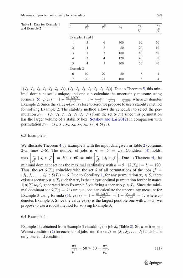
Let the input data for Example 1 of problem 1|pLi ≤ pi ≤ pU

i | ∑wi Ci with n = 5 =n1 be given in Table 1 (columns 2–5, lines 2–6). The weight-to-process ratios for theprocessing times which are equal to the lower (upper) bounds are given in column 6(column 7). We test condition (2):

w3

pU3

≥ w1

pL1

; w1

pU1

≥ w5

pL5

; w5

pU5

≥ w4

pL4

; w4

pU4

>w2

pL2

. (10)

Since conditions (2) are transitive, we do not present them, if they may be obtainedvia the transitivity from those already presented in (10).

Since condition (3) of Theorem 3 holds, the minimal dominant set S(T1) is asingleton: S(T1) = {πk}, where the scenario set T1 is defined in Table 1 (columns2–5, lines 2–6) and πk = (J3, J1, J5, J4, J2). The permutation πk is obtained due tothe WSPT rule used for the ordering of the jobs J with the processing times pi = pL

i(or pi = pU

i ) of a job Ji ∈ J (due to (3) in both cases, the same permutation πk

is obtained). The permutation πk is optimal for any instance 1|p|∑ wi Ci generatedfrom Example 1 via fixing a scenario p ∈ T1. We calculate the uncertainty measureusing formula (5): ϕ(z1) = 1 − n!−|S(T1)|

n!−1 = 1 − 5!−15!−1 = 0. Here the instance z1

denotes Example 1. A zero value of the uncertainty measure means that there is noinfluence of the uncertainty while one looks for a solution to such a problem.

6.2 Example 2

Example 2 is obtained from Example 1 by adding the jobs J6 and J7 (Table 1).The number of jobs is n = 7 = n2. After checking the validity of condition(2) for all jobs Ju ∈ {J1, J2, . . . , J5} and jobs Jv ∈ {J6, J7}, we obtain theconditions wu

pUu

> w6pL

6and wu

pUu

> w7pL

7in addition to conditions (10). For Exam-

ple 2, condition (3) does not hold since job J6 does not dominate job J7 (Theo-rem 2) and vice versa. A minimal dominant set is as follows: S(T2) = {πh, πl} =

123


Table 1 Data for Example 1and Example 2 i pL

i pUi wi

wi

pLi

wi

pUi

Examples 1 and 2

1 5 6 300 60 50

2 4 8 80 20 10

3 1 3 180 180 60

4 3 4 120 40 30

5 4 5 200 50 40

Example 2

6 10 20 80 8 4

7 20 25 100 5 4

{(J3, J1, J5, J4, J2, J6, J7), (J3, J1, J5, J4, J2, J7, J6)}. Due to Theorem 5, this min-imal dominant set is unique, and one can calculate the uncertainty measure usingformula (5): ϕ(z2) = 1 − n!−|S(T2)|

n!−1 = 1 − 7!−27!−1 = 1

7!−1 = 15,039 , where z2 denotes

Example 2. Since the value ϕ(z2) is close to zero, we propose to use a stability methodfor solving Example 2. The stability method allows the scheduler to select the per-mutation πh = (J3, J1, J5, J4, J2, J7, J6) from the set S(T2) since this permutationhas the larger volume of a stability box (Sotskov and Lai 2012) in comparison withpermutation πl = (J3, J1, J5, J4, J2, J6, J7) ∈ S(T2).

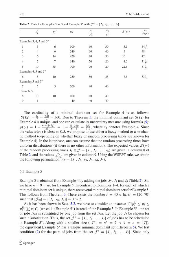
6.3 Example 3

We illustrate Theorem 4 by Example 3 with the input data given in Table 2 (columns2–5, lines 2–6). The number of jobs is n = 5 = n3. Condition (4) holds:

max

{wipU

i| Ji ∈ J

}

= 50 < 60 = min

{wipL

i| Ji ∈ J

}

. Due to Theorem 4, the

minimal dominant set has the maximal cardinality with n = 5 : |S(T3)| = 5! = 120.

Thus, the set S(T3) coincides with the set S of all permutations of the jobs J ={J1, J2, . . . , J5} : S(T3) = S. Due to Corollary 1, for any permutation πk ∈ S, thereexists a scenario p ∈ T3 such that πk is the unique optimal permutation for the instance1|p| ∑wi Ci generated from Example 3 via fixing a scenario p ∈ T3. Since the mini-mal dominant set S(T3) = S is unique, one can calculate the uncertainty measure forExample 3 using formula (5): ϕ(z3) = 1 − n!−|S(T3)|

n!−1 = 1 − 5!−1205!−1 = 1, where z3

denotes Example 3. Since the value ϕ(z3) is the largest possible one with n = 5, wepropose to use a robust method for solving Example 3.

6.4 Example 4

Example 4 is obtained from Example 3 via adding the job J6 (Table 2). So, n = 6 = n4.

We test condition (2) for each pair of jobs from the set J = {J1, J2, . . . , J6} and obtainonly one valid condition:

w1

pU1

= 50 ≥ 50 = w6

pL6

. (11)

123


Table 2 Data for Examples 3, 4, 5 and Example 5∗ with J ∗ = {J1, J2, . . . , J7}

i pLi pU

i wiwi

pLi

wi

pUi

E(pi )wi

E(pi )

Examples 3, 4, 5 and 5∗

1 5 6 300 60 50 5.5 54 611

2 4 6 240 60 40 5 48

3 6 14 420 70 30 10 42

4 2 7 140 70 20 4.5 31 19

5 10 35 700 70 20 22.5 31 19

Examples 4, 5 and 5∗

6 5 10 250 50 25 7.5 33 13

Examples 5 and 5∗7 5 5 200 40 40

Example 5

8 10 10 400 40 40

9 1 1 40 40 40

The cardinality of a minimal dominant set for Example 4 is as follows:|S(T4)| = 6!

2 = 7202 = 360. Due to Theorem 5, the minimal dominant set S(T4) for

Example 4 is unique, and one can calculate its uncertainty measure using formula (5):ϕ(z4) = 1 − n!−|S(T4)|

n!−1 = 1 − 6!−3606!−1 = 359

719 , where z4 denotes Example 4. Sincethe value ϕ(z4) is close to 0.5, we propose to use either a fuzzy method or a stochas-tic method (depending on whether fuzzy or random processing times are known forExample 4). In the latter case, one can assume that the random processing times haveuniform distributions (if there is no other information). The expected values E(pi )

of the random processing times Ji ∈ J = {J1, J2, . . . , J6} are given in column 8 ofTable 2, and the values wi

E(pi )are given in column 9. Using the WSEPT rule, we obtain

the following permutation: πh = (J1, J2, J3, J6, J4, J5).

6.5 Example 5

Example 5 is obtained from Example 4 by adding the jobs J7, J8 and J9 (Table 2). So,we have n = 9 = n5 for Example 5. In contrast to Examples 1–4, for each of which aminimal dominant set is unique, there are several minimal dominant sets for Example 5.This follows from Theorem 5: There exists the number r = 40 ∈ [a, b] = [20, 70]such that |J40| = |{J7, J8, J9}| = 3 > 2.

As it has been shown in Sect. 5.2, we have to consider an instance 1∗|pLi ≤ pi ≤

pUi | ∑wi Ci (we call it Example 5∗) instead of the Example 5. In Example 5∗, the set

of jobs J40 is substituted by one job from the set J40. Let the job J7 be chosen forsuch a substitution. Thus, the set J ∗ = {J1, J2, . . . , J7} of jobs has to be scheduledin Example 5∗. Along with a smaller size (|J ∗| = n∗ = 7 < 9 = n = |J |),the equivalent Example 5∗ has a unique minimal dominant set (Theorem 5). We testcondition (2) for the pairs of jobs from the set J ∗ = {J1, J2, . . . , J7}. Since only

123


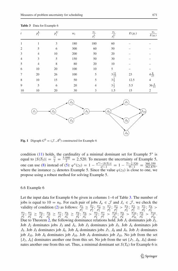
Table 3 Data for Example 6

i pLi pU

i wiwi

pLi

wi

pUi

E(pi )wi

E(pi )

1 1 3 180 180 60 – –

2 5 6 300 60 50 – –

3 4 10 200 50 20 – –

4 3 5 150 50 30 – –

5 4 8 80 20 10 – –

6 10 20 100 10 5 – –

7 20 26 100 5 3 1113 23 4 8

23

8 10 15 50 5 3 23 12.5 4

9 5 6 20 4 3 13 5.5 36 4

1110 10 20 30 3 1.5 15 2

Fig. 1 Digraph G0 = (J , A0) constructed for Example 6

condition (11) holds, the cardinality of a minimal dominant set for Example 5∗ isequal to |S(T5)| = 7!

2 = 5,0402 = 2,520. To measure the uncertainty of Example 5,

one can use (8) instead of (5): ϕ∗(z5) = 1 − n∗!−|S(T5)|n!−1 = 1 − 7!−2,520

9!−1 = 360,359362,879 ,

where the instance z5 denotes Example 5. Since the value ϕ(z5) is close to one, wepropose using a robust method for solving Example 5.

6.6 Example 6

Let the input data for Example 6 be given in columns 1–4 of Table 3. The number ofjobs is equal to 10 = n6. For each pair of jobs Ju ∈ J and Jv ∈ J , we check thevalidity of condition (2) as follows: w1

pU1

≥ w2pL

2; w2

pU2

≥ w3pL

3; w2

pU2

> w4pL

4; w3

pU3

≥ w5pL

5; w4

pU4

>

w5pL

5; w5

pU5

≥ w6pL

6; w6

pU6

≥ w7pL

7; w6

pU6

≥ w8pL

8; w6

pU6

> w9pL

9; w7

pU7

> w10pL

10; w8

pU8

> w10pL

10; w9

pU9

> w10pL

10.

Due to Theorem 2, the following dominance relations hold. Job J1 dominates job J2.

Job J2 dominates jobs J3 and J4. Job J3 dominates job J5. Job J4 dominates jobJ5. Job J5 dominates job J6. Job J6 dominates jobs J7, J8 and J9. Job J7 dominatesjob J10. Job J8 dominates job J10. Job J9 dominates job J10. No job from the set{J3, J4} dominates another one from this set. No job from the set {J7, J8, J9} domi-nates another one from this set. Thus, a minimal dominant set S(T6) for Example 6 is

123


defined by the digraph G = (J ,A). In Fig. 1, the reduction digraph G0 = (J ,A0) ofthe digraph G = (J ,A) is presented. (The digraph G0 is obtained from digraph G bydeleting the transitive arcs.) Example 6 may be decomposed into two subproblems. Inthe first subproblem, the set of jobs {J1, J2, . . . , J6} has to be scheduled (we call thissubproblem as instance z7). In the second subproblem, the set of jobs {J7, J8, J9, J10}has to be scheduled (we call this subproblem as instance z8). We have n7 = 6, n8 = 4and calculate the values ϕ(z7), ϕ(z8) using formula (5): ϕ(z7) = 1 − 6!−|S(T7)|

6!−1 =1− 720−2

720−1 = 1719 , ϕ(z8) = 1− 4!−|S(T8)|

4!−1 = 1− 24−624−1 = 5

23 . Due to the above values ofthe uncertainty measure, we propose to use a stability method for solving the instancez7, and a stochastic method (or a fuzzy method) for solving the instance z8 (dependingon whether fuzzy or random processing times are known). For the instance z7, thestability method allows the scheduler to select the permutation (J1, J2, J4, J3, J5, J6)

having the larger volume of a stability box (Sotskov and Lai 2012) in comparison withpermutation (J1, J2, J3, J4, J5, J6). Let a stochastic method be used for the instancez8. One can assume that the random processing times have uniform distributions.The expected values E(pi ) of the random processing times Ji ∈ {J7, J8, J9, J10}are given in column 7 of Table 3, and the values wi

E(pi )are given in column 8.

Using the WSEPT rule, we obtain permutation: (J9, J7, J8, J10). The job permutation(J1, J2, J4, J3, J5, J6, J9, J7, J8, J10) for the whole instance z6 is defined via con-catenating the permutations (J1, J2, J4, J3, J5, J6) and (J9, J7, J8, J10). Example 6demonstrates that an instance 1|pL

i ≤ pi ≤ pUi | ∑wi Ci may need several methods,

if it has parts with different values of the uncertainty measure.

6.7 Calculation of the uncertainty measure μ(zk)

Since it is impossible to generate all elements of a set S(T ) in polynomial time of n,

the calculation of the measure ϕ(zk) or ϕ∗(zk) based on the cardinality |S(T )| may betime-consuming for a large n. So, the calculation of μ(zk) is preferable in comparisonwith the calculation of ϕ(zk) or ϕ∗(zk). The measure μ(zk) is based on the cardinalityof the set of arcs Ak in the dominance digraph Gk = (J ,Ak) constructed for theinstance zk . Using (9), we calculate the values of the measure μ(zk) for the exampleszk ∈ Z, k ∈ {1, 2, . . . , 8}, as follows: μ(z1) = 1− 2|A1|

n1(n1−1)= 1− 2·10

5(5−1)=0;μ(z2) =

1 − 2|A2|n2(n2−1)

= 121 ;μ(z3) = 1 − 2|A3|

n3(n3−1)= 1;μ(z4) = 1 − 2|A4|

n4(n4−1)= 14

15 ;μ(z5) =1 − 2|A5|

n5(n5−1)= 35

36 ;μ(z7) = 1 − 2|A7|n7(n7−1)

= 115 ;μ(z8) = 1 − 2|A8|

n8(n8−1)= 0.5.

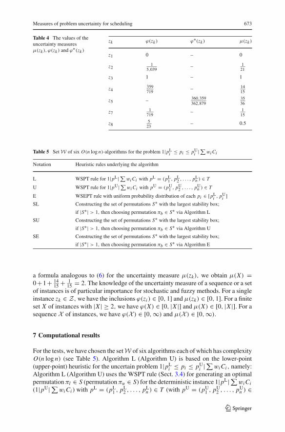
The values of the uncertainty measures μ(zk), ϕ(zk) and ϕ∗(zk) for the instanceszk, k ∈ {1, 2, 3, 4, 5, 7, 8}, are given in Table 4.

6.8 Calculation of the uncertainty measure for a sequence of instances

If one needs to solve a sequence (or a set) of instances, then formula (6) [or (7)] has to beused for calculating the uncertainty measure of a sequence (a set) of instances insteadof formula (5) used to measure the uncertainty of a single instance. For example, forthe set X = {z1, z3, z4, z7}, we obtain ϕ(X) = 0 + 1 + 369

719 + 1719 = 1 360

719 . Using

123


Table 4 The values of theuncertainty measuresμ(zk ), ϕ(zk ) and ϕ∗(zk )

zk ϕ(zk ) ϕ∗(zk ) μ(zk )

z1 0 – 0

z21

5,039– 1

21

z3 1 – 1

z4359719

– 1415

z5 – 360,359362,879

3536

z71

719– 1

15

z85

23– 0.5

Table 5 Set W of six O(n log n)-algorithms for the problem 1|pLi ≤ pi ≤ pU

i | ∑ wi Ci

Notation Heuristic rules underlying the algorithm

L WSPT rule for 1|pL| ∑ wi Ci with pL = (pL1 , pL

2 , . . . , pLn ) ∈ T

U WSPT rule for 1|pU| ∑ wi Ci with pU = (pU1 , pU

2 , . . . , pUn ) ∈ T

E WSEPT rule with uniform probability distribution of each pi ∈ [pLi , pU

i ]SL Constructing the set of permutations S∗ with the largest stability box;

if |S∗| > 1, then choosing permutation πb ∈ S∗ via Algorithm L

SU Constructing the set of permutations S∗ with the largest stability box;

if |S∗| > 1, then choosing permutation πb ∈ S∗ via Algorithm U

SE Constructing the set of permutations S∗ with the largest stability box;

if |S∗| > 1, then choosing permutation πb ∈ S∗ via Algorithm E

a formula analogous to (6) for the uncertainty measure μ(zk), we obtain μ(X) =0+1+ 14

15 + 115 = 2. The knowledge of the uncertainty measure of a sequence or a set

of instances is of particular importance for stochastic and fuzzy methods. For a singleinstance zk ∈ Z, we have the inclusions ϕ(zi ) ∈ [0, 1] and μ(zk) ∈ [0, 1]. For a finiteset X of instances with |X | ≥ 2, we have ϕ(X) ∈ [0, |X |] and μ(X) ∈ [0, |X |]. For asequence X of instances, we have ϕ(X ) ∈ [0,∞) and μ(X ) ∈ [0,∞).

7 Computational results

For the tests, we have chosen the set W of six algorithms each of which has complexityO(n log n) (see Table 5). Algorithm L (Algorithm U) is based on the lower-point(upper-point) heuristic for the uncertain problem 1|pL

i ≤ pi ≤ pUi | ∑wi Ci , namely:

Algorithm L (Algorithm U) uses the WSPT rule (Sect. 3.4) for generating an optimalpermutation πl ∈ S (permutation πu ∈ S) for the deterministic instance 1|pL| ∑ wi Ci

(1|pU| ∑ wi Ci ) with pL = (pL1 , pL

2 , . . . , pLn ) ∈ T (with pU = (pU

1 , pU2 , . . . , pU

n ) ∈

123


T, respectively). The stochastic Algorithm E realizes the WSEPT rule (Sect. 3.2)with the assumption of a uniform probability distribution for the random processingtime pi within the segment [pL

i , pUi ]. The stability method constructs a set S∗ ⊆ S

of permutations with the largest relative volume of a stability box (Sotskov and Lai2012). Since there might be several permutations with the largest volume of a stabilitybox, i.e., |S∗| > 1, the stability method was combined with the lower-point heuristic(this combination of two heuristics is called Algorithm SL), with the upper-pointheuristic (this combination is called Algorithm SU) and with a stochastic algorithm(this combination is called Algorithm SE).

Algorithms L, U, E, SL, SU and SE were coded in C++ and tested on a PC withAMD Athlon (tm) 64 Processor 3,200+, 2.00 GHz, 1.96 GB of RAM.

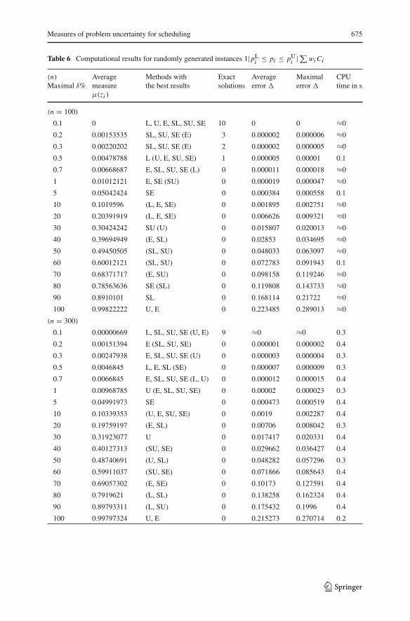
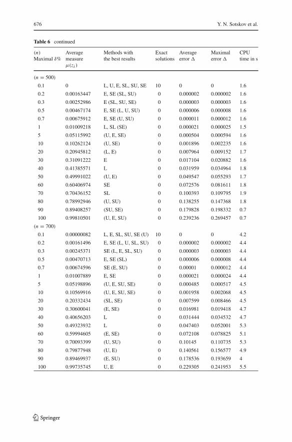
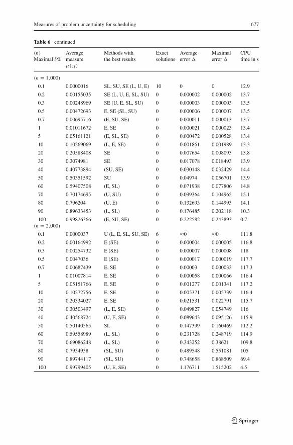
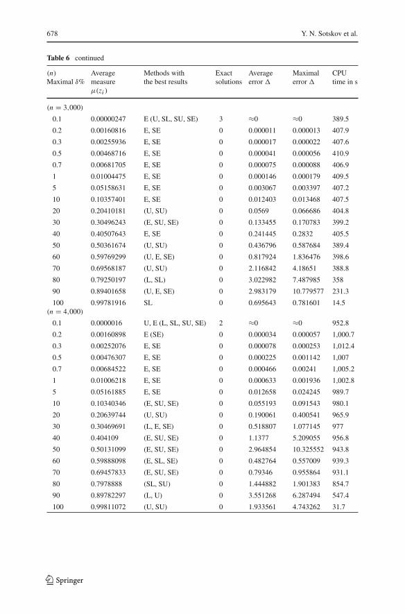
Table 6 represents the computational results for series of randomly generatedinstances 1|pL

i ≤ pi ≤ pUi | ∑wi Ci with n ∈ {100, 300, 500, 700, 1,000, 2,000,

3,000, 4,000, 5,000}. Each series contains ten randomly generated instances withthe same number n of jobs and the same maximal possible error δ% of the randomprocessing times. The number n is given in parenthesis before the corresponding partof Table 6. The integer lower and upper bounds pL

i and pUi on the processing times

pi ∈ [pLi , pU

i ] have been generated as follows.An integer center C of a segment [pL

i , pUi ] was generated using the uniform dis-

tribution in the range [L , U ] : L ≤ C ≤ U. The lower bound was defined aspL

i = C · (1 − δ100 ) and the upper bound as pU

i = C · (1 + δ100 ). The maximum

possible error of the random processing time in percentages is equal to δ% given incolumn 1 of Table 6. The same range [L , U ] = [1, 500] for the varying center C wasused for all jobs Ji ∈ J in all instances presented in Table 6. For each job Ji ∈ J , theweight wi was uniformly distributed in the range [1, 50]. (In contrast to the processingtimes pi , the weights wi were assumed to be known precisely before scheduling.) Thecomputational experiments were aimed to answer the following two questions. Whichalgorithms of the six ones tested give the best objective function value for a series ofinstances? How large may the error of the optimal value of the objective function beprovided by such an algorithm for the concrete scheduling problem?

The average value of the measure μ(zk) for the 10 instances in a series is givenin column 2 of Table 6. Columns 3 indicates one or several algorithms providing thebest value of the objective function γ = ∑

Ji ∈J wi Ci for a series of instances. Thebest results obtained by such algorithms are characterized in columns 4–6. Column 4presents the number of instances (from 10 ones in a series) solved exactly by the bestalgorithm for this series. Column 5 (column 6) presents the average (maximal) relative

error � obtained by the best algorithm: � = γ tp∗−γ ∗

p∗γ ∗

p∗ , where γ tp∗ denotes the value of

the objective function γ = ∑Ji ∈J wi Ci for the permutation πt constructed by the best

algorithm. The value γ ∗p∗ denotes the ex-post optimal value of the objective function,

i.e., that calculated for the instance 1|p∗| ∑ wi Ci , where p∗ = (p∗1, p∗

2, . . . , p∗n) ∈ T

is the actual scenario (unknown before scheduling).The best algorithm or algorithms (indicated in column 3) provide the best results for

all three characteristics presented in columns 4–6. If for a series, there is no algorithmwith the best of all three characteristics, then the algorithms providing Pareto optimalcharacteristics are indicated in column 3 in parenthesis. For example, the line of Table 6

123


Table 6 Computational results for randomly generated instances 1|pLi ≤ pi ≤ pU

i | ∑ wi Ci

(n)

Maximal δ%Averagemeasureμ(zi )

Methods withthe best results

Exactsolutions

Averageerror �

Maximalerror �

CPUtime in s

(n = 100)

0.1 0 L, U, E, SL, SU, SE 10 0 0 ≈0

0.2 0.00153535 SL, SU, SE (E) 3 0.000002 0.000006 ≈0

0.3 0.00220202 SL, SU, SE (E) 2 0.000002 0.000005 ≈0

0.5 0.00478788 L (U, E, SU, SE) 1 0.000005 0.00001 0.1

0.7 0.00668687 E, SL, SU, SE (L) 0 0.000011 0.000018 ≈0

1 0.01012121 E, SE (SU) 0 0.000019 0.000047 ≈0

5 0.05042424 SE 0 0.000384 0.000558 0.1

10 0.1019596 (L, E, SE) 0 0.001895 0.002751 ≈0

20 0.20391919 (L, E, SE) 0 0.006626 0.009321 ≈0

30 0.30424242 SU (U) 0 0.015807 0.020013 ≈0

40 0.39694949 (E, SL) 0 0.02853 0.034695 ≈0

50 0.49450505 (SL, SU) 0 0.048033 0.063097 ≈0

60 0.60012121 (SL, SU) 0 0.072783 0.091943 0.1

70 0.68371717 (E, SU) 0 0.098158 0.119246 ≈0

80 0.78563636 SE (SL) 0 0.119808 0.143733 ≈0

90 0.8910101 SL 0 0.168114 0.21722 ≈0

100 0.99822222 U, E 0 0.223485 0.289013 ≈0

(n = 300)

0.1 0.00000669 L, SL, SU, SE (U, E) 9 ≈0 ≈0 0.3

0.2 0.00151394 E (SL, SU, SE) 0 0.000001 0.000002 0.4

0.3 0.00247938 E, SL, SU, SE (U) 0 0.000003 0.000004 0.3

0.5 0.0046845 L, E, SL (SE) 0 0.000007 0.000009 0.3

0.7 0.0066845 E, SL, SU, SE (L, U) 0 0.000012 0.000015 0.4

1 0.00968785 U (E, SL, SU, SE) 0 0.00002 0.000023 0.3

5 0.04991973 SE 0 0.000473 0.000519 0.4

10 0.10339353 (U, E, SU, SE) 0 0.0019 0.002287 0.4

20 0.19759197 (E, SL) 0 0.00706 0.008042 0.3

30 0.31923077 U 0 0.017417 0.020331 0.4

40 0.40127313 (SU, SE) 0 0.029662 0.036427 0.4

50 0.48740691 (U, SL) 0 0.048282 0.057296 0.3

60 0.59911037 (SU, SE) 0 0.071866 0.085643 0.4

70 0.69057302 (E, SE) 0 0.10173 0.127591 0.4

80 0.7919621 (L, SL) 0 0.138258 0.162324 0.4

90 0.89793311 (L, SU) 0 0.175432 0.1996 0.4

100 0.99797324 U, E 0 0.215273 0.270714 0.2

123


Table 6 continued

(n)



Exactsolutions

Averageerror �

Maximalerror �

CPUtime in s

(n = 500)

0.1 0 L, U, E, SL, SU, SE 10 0 0 1.6

0.2 0.00163447 E, SE (SL, SU) 0 0.000002 0.000002 1.6

0.3 0.00252986 E (SL, SU, SE) 0 0.000003 0.000003 1.6

0.5 0.00467174 E, SE (L, U, SU) 0 0.000006 0.000008 1.6

0.7 0.00675912 E, SE (U, SU) 0 0.000011 0.000012 1.6

1 0.01009218 L, SL (SE) 0 0.000021 0.000025 1.5

5 0.05115992 (U, E, SE) 0 0.000504 0.000594 1.6

10 0.10262124 (U, SE) 0 0.001896 0.002235 1.6

20 0.20945812 (L, E) 0 0.007964 0.009152 1.7

30 0.31091222 E 0 0.017104 0.020882 1.6

40 0.41385571 L 0 0.031959 0.034964 1.8

50 0.49991022 (U, E) 0 0.049547 0.055293 1.7

60 0.60406974 SE 0 0.072576 0.081611 1.8

70 0.70436152 SL 0 0.100393 0.109795 1.9

80 0.78992946 (U, SU) 0 0.138255 0.147368 1.8

90 0.89408257 (SU, SE) 0 0.179828 0.198332 0.7

100 0.99810501 (U, E, SU) 0 0.239236 0.269457 0.7

(n = 700)

0.1 0.00000082 L, E, SL, SU, SE (U) 10 0 0 4.2

0.2 0.00161496 E, SE (L, U, SL, SU) 0 0.000002 0.000002 4.4

0.3 0.00245371 SE (L, E, SL, SU) 0 0.000003 0.000003 4.4

0.5 0.00470713 E, SE (SL) 0 0.000006 0.000008 4.4

0.7 0.00674596 SE (E, SU) 0 0.00001 0.000012 4.4

1 0.01007889 E, SE 0 0.000021 0.000024 4.4

5 0.05198896 (U, E, SU, SE) 0 0.000485 0.000517 4.5

10 0.10569916 (U, E, SU, SE) 0 0.001958 0.002068 4.5

20 0.20332434 (SL, SE) 0 0.007599 0.008466 4.5

30 0.30600041 (E, SE) 0 0.016981 0.019418 4.7

40 0.40656203 L 0 0.031444 0.034532 4.7

50 0.49323932 L 0 0.047403 0.052001 5.3

60 0.59994605 (E, SE) 0 0.072108 0.078825 5.1

70 0.70093399 (U, SU) 0 0.10145 0.110735 5.3

80 0.79877948 (U, E) 0 0.140561 0.156577 4.9

90 0.89469937 (E, SU) 0 0.178536 0.193659 4

100 0.99735745 U, E 0 0.229305 0.241953 5.5

123


Table 6 continued

(n)



Exactsolutions

Averageerror �

Maximalerror �

CPUtime in s

(n = 1,000)

0.1 0.0000016 SL, SU, SE (L, U, E) 10 0 0 12.9

0.2 0.00155035 SE (L, U, E, SL, SU) 0 0.000002 0.000002 13.7

0.3 0.00248969 SE (U, E, SL, SU) 0 0.000003 0.000003 13.5

0.5 0.00472693 E, SE (SL, SU) 0 0.000006 0.000007 13.5

0.7 0.00695716 (E, SU, SE) 0 0.000011 0.000013 13.7

1 0.01011672 E, SE 0 0.000021 0.000023 13.4

5 0.05161121 (E, SL, SE) 0 0.000472 0.000528 13.4

10 0.10269069 (L, E, SE) 0 0.001861 0.001989 13.3

20 0.20588408 SE 0 0.007654 0.008093 13.8

30 0.3074981 SE 0 0.017078 0.018493 13.9

40 0.40773894 (SU, SE) 0 0.030148 0.032429 14.4

50 0.50351592 SU 0 0.04974 0.056701 13.9

60 0.59407508 (E, SL) 0 0.071938 0.077806 14.8

70 0.70174695 (U, SU) 0 0.099364 0.104965 15.1

80 0.796204 (U, E) 0 0.132693 0.144993 14.1

90 0.89633453 (L, SL) 0 0.176485 0.202118 10.3

100 0.99826366 (E, SU, SE) 0 0.222582 0.243893 0.7(n = 2,000)

0.1 0.0000037 U (L, E, SL, SU, SE) 6 ≈0 ≈0 111.8

0.2 0.00164992 E (SE) 0 0.000004 0.000005 116.8

0.3 0.00254732 E (SE) 0 0.000007 0.000008 118

0.5 0.0047036 E (SE) 0 0.000017 0.000019 117.7

0.7 0.00687439 E, SE 0 0.00003 0.000033 117.3

1 0.01007814 E, SE 0 0.000058 0.000066 116.4

5 0.05151766 E, SE 0 0.001277 0.001341 117.2

10 0.10272756 E, SE 0 0.005371 0.005739 116.4

20 0.20334027 E, SE 0 0.021531 0.022791 115.7

30 0.30503497 (L, E, SE) 0 0.049827 0.054749 116

40 0.40568724 (U, E, SE) 0 0.089643 0.095126 115.9

50 0.50140565 SL 0 0.147399 0.160469 112.2

60 0.59558989 (L, SL) 0 0.231728 0.248719 114.9

70 0.69086248 (L, SL) 0 0.343252 0.38621 109.8

80 0.7934938 (SL, SU) 0 0.489548 0.551081 105

90 0.89744117 (SL, SU) 0 0.748658 0.868509 69.4

100 0.99799405 (U, E, SE) 0 1.176711 1.515202 4.5

123


Table 6 continued

(n)



Exactsolutions

Averageerror �

Maximalerror �

CPUtime in s

(n = 3,000)

0.1 0.00000247 E (U, SL, SU, SE) 3 ≈0 ≈0 389.5

0.2 0.00160816 E, SE 0 0.000011 0.000013 407.9

0.3 0.00255936 E, SE 0 0.000017 0.000022 407.6

0.5 0.00468716 E, SE 0 0.000041 0.000056 410.9

0.7 0.00681705 E, SE 0 0.000075 0.000088 406.9

1 0.01004475 E, SE 0 0.000146 0.000179 409.5

5 0.05158631 E, SE 0 0.003067 0.003397 407.2

10 0.10357401 E, SE 0 0.012403 0.013468 407.5

20 0.20410181 (U, SU) 0 0.0569 0.066686 404.8

30 0.30496243 (E, SU, SE) 0 0.133455 0.170783 399.2

40 0.40507643 E, SE 0 0.241445 0.2832 405.5

50 0.50361674 (U, SU) 0 0.436796 0.587684 389.4

60 0.59769299 (U, E, SE) 0 0.817924 1.836476 398.6

70 0.69568187 (U, SU) 0 2.116842 4.18651 388.8

80 0.79250197 (L, SL) 0 3.022982 7.487985 358

90 0.89401658 (U, E, SE) 0 2.983179 10.779577 231.3

100 0.99781916 SL 0 0.695643 0.781601 14.5(n = 4,000)

0.1 0.0000016 U, E (L, SL, SU, SE) 2 ≈0 ≈0 952.8

0.2 0.00160898 E (SE) 0 0.000034 0.000057 1,000.7

0.3 0.00252076 E, SE 0 0.000078 0.000253 1,012.4

0.5 0.00476307 E, SE 0 0.000225 0.001142 1,007

0.7 0.00684522 E, SE 0 0.000466 0.00241 1,005.2

1 0.01006218 E, SE 0 0.000633 0.001936 1,002.8

5 0.05161885 E, SE 0 0.012658 0.024245 989.7

10 0.10340346 (E, SU, SE) 0 0.055193 0.091543 980.1

20 0.20639744 (U, SU) 0 0.190061 0.400541 965.9

30 0.30469691 (L, E, SE) 0 0.518807 1.077145 977

40 0.404109 (E, SU, SE) 0 1.1377 5.209055 956.8

50 0.50131099 (E, SU, SE) 0 2.964854 10.325552 943.8

60 0.59888098 (E, SL, SE) 0 0.482764 0.557009 939.3

70 0.69457833 (E, SU, SE) 0 0.79346 0.955864 931.1

80 0.7978888 (SL, SU) 0 1.444882 1.901383 854.7

90 0.89782297 (L, U) 0 3.551268 6.287494 547.4

100 0.99811072 (U, SU) 0 1.933561 4.743262 31.7

123


Table 6 continued

(n)



Exactsolutions

Averageerror �

Maximalerror �

CPUtime in s

(n = 5,000)

0.1 0.00000201 E, SL, SU, SE (L, U) 1 ≈0 ≈0 1,950.9

0.2 0.00159402 E, SE 0 0.000021 0.000023 2,035

0.3 0.00253486 E (SE) 0 0.000044 0.000096 2,045.1

0.5 0.00475245 E (SE) 0 0.001461 0.013593 2,022.2

0.7 0.00688566 E (SE) 0 0.000299 0.001262 2,018.6

1 0.01016814 SE (E) 0 0.000695 0.00367 2,038.9

5 0.05147954 E, SE 0 0.005636 0.006811 2,059.7

10 0.10271562 (U, E, SE) 0 0.024547 0.030565 1,968.5

20 0.20644317 (E, SU, SE) 0 0.097151 0.130148 1,892.1

30 0.30734107 (L, U) 0 0.265321 0.386807 1,924.3

40 0.40436974 (U, SU) 0 0.647339 1.192235 1,873.5

50 0.50312959 (E, SL, SE) 0 1.294992 2.305626 1,899.9

60 0.59650079 (E, SU, SE) 0 1.761138 3.729997 1,847.8

70 0.69465952 E, SE 0 1.639203 6.923092 1,827.7

80 0.79293199 (E, SU, SE) 0 0.273271 0.362255 1,633.3

90 0.89629171 (E, SU, SE) 0 1.718265 2.642256 1,012

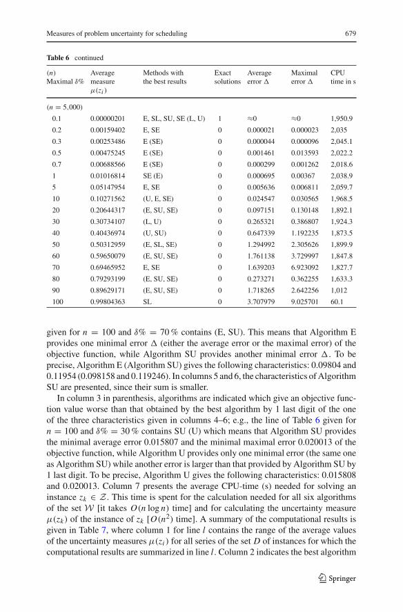
100 0.99804363 SL 0 3.707979 9.025701 60.1

given for n = 100 and δ% = 70 % contains (E, SU). This means that Algorithm Eprovides one minimal error � (either the average error or the maximal error) of theobjective function, while Algorithm SU provides another minimal error �. To beprecise, Algorithm E (Algorithm SU) gives the following characteristics: 0.09804 and0.11954 (0.098158 and 0.119246). In columns 5 and 6, the characteristics of AlgorithmSU are presented, since their sum is smaller.

In column 3 in parenthesis, algorithms are indicated which give an objective func-tion value worse than that obtained by the best algorithm by 1 last digit of the oneof the three characteristics given in columns 4–6; e.g., the line of Table 6 given forn = 100 and δ% = 30 % contains SU (U) which means that Algorithm SU providesthe minimal average error 0.015807 and the minimal maximal error 0.020013 of theobjective function, while Algorithm U provides only one minimal error (the same oneas Algorithm SU) while another error is larger than that provided by Algorithm SU by1 last digit. To be precise, Algorithm U gives the following characteristics: 0.015808and 0.020013. Column 7 presents the average CPU-time (s) needed for solving aninstance zk ∈ Z. This time is spent for the calculation needed for all six algorithmsof the set W [it takes O(n log n) time] and for calculating the uncertainty measureμ(zk) of the instance of zk [O(n2) time]. A summary of the computational results isgiven in Table 7, where column 1 for line l contains the range of the average valuesof the uncertainty measures μ(zi ) for all series of the set D of instances for which thecomputational results are summarized in line l. Column 2 indicates the best algorithm

123


Table 7 Summary of the computational results

l Range of the averagevalues of measure μ(zi )


Minimalaver. error

Maximalaver. error

Maximalerror �

Number of jobs n ∈ {100, 300, 500, 700, 1,000}1 2 3 4 5

1 [0, 0.00252986] E, SL, SU, SE 0 0.000003 0.000006

2 [0.00478788, 0.10569916] SE 0.000005 0.001958 0.002751

3 [0.19759197, 0.20945812] (E ∨ SE) 0.006626 0.007964 0.009321

4 [0.30424242, 0.31923077] (L ∨ SL ∨ SU) 0.015807 0.017417 0.020882

5 [0.39694949, 0.41385571] (U ∨ E ∨ SE) 0.02853 0.031959 0.036427

6 [0.48740691, 0.50351592] (L ∨ E ∨ SU) 0.047403 0.04974 0.063097

7 [0.59407508, 0.60406974] (SL ∨ SE) 0.071866 0.072783 0.091943

8 [0.68371717, 0.70436152] (SL ∨ SU ∨ SE) 0.098158 0.10173 0.127591

9 [0.78563636, 0.79877948] (SL ∨ SU) 0.119808 0.140561 0.162324

10 [0.8910101, 0.89793311] (U ∨ SU) 0.168114 0.179828 0.21722

11 [0.99735745, 0.99826366] E 0.215273 0.239236 0.289013

Number of jobs n ∈ {2,000, 3,000, 4,000, 5,000}12 [0.0000016, 0.0000037] U, E, SL, SU, SE ≈0 ≈0 ≈0

13 [0.00159402, 0.10357401] E, SE 0.000004 0.055193 0.091543

14 [0.20334027, 0.10569916] (SU ∨ SE) 0.021531 0.190061 0.400541

15 [0.30496243, 0.30734107] (L ∨ SE) 0.049827 0.518807 1.077145

16 [0.404109, 0.40568724] (SU ∨ SE) 0.089643 1.1377 5.209055

17 [0.50131099, 0.50361674] (SL ∨ SU) 0.147399 2.964854 10.325552

18 [0.59558989, 0.59888098] (SL ∨ SE) 0.231728 1.761138 3.729997

19 [0.69086248, 0.69568187] (SL ∨ SU ∨ SE) 0.343252 2.116842 6.923092

20 [0.79250197, 0.7978888] (SL ∨ SU) 0.273271 3.022982 7.487985

21 [0.89401658, 0.89782297] (U ∨ SU) 0.748658 2.983179 10.779577

22 [0.99781916, 0.99811072] (U ∨ SL) 0.695643 3.707979 9.025701

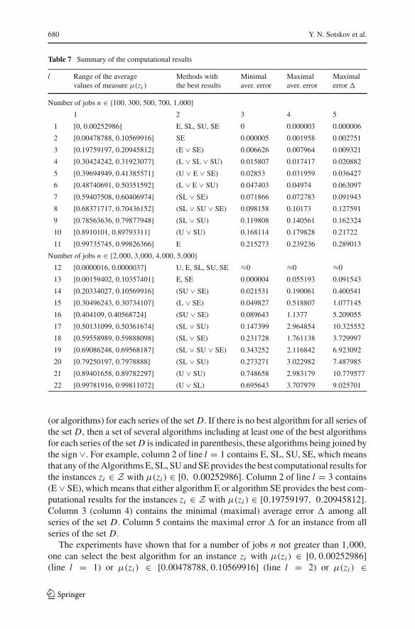
(or algorithms) for each series of the set D. If there is no best algorithm for all series ofthe set D, then a set of several algorithms including at least one of the best algorithmsfor each series of the set D is indicated in parenthesis, these algorithms being joined bythe sign ∨. For example, column 2 of line l = 1 contains E, SL, SU, SE, which meansthat any of the Algorithms E, SL, SU and SE provides the best computational results forthe instances zi ∈ Z with μ(zi ) ∈ [0, 0.00252986]. Column 2 of line l = 3 contains(E ∨ SE), which means that either algorithm E or algorithm SE provides the best com-putational results for the instances zi ∈ Z with μ(zi ) ∈ [0.19759197, 0.20945812].Column 3 (column 4) contains the minimal (maximal) average error � among allseries of the set D. Column 5 contains the maximal error � for an instance from allseries of the set D.

The experiments have shown that for a number of jobs n not greater than 1,000,

one can select the best algorithm for an instance zi with μ(zi ) ∈ [0, 0.00252986](line l = 1) or μ(zi ) ∈ [0.00478788, 0.10569916] (line l = 2) or μ(zi ) ∈

123


[0.99735745, 0.99826366] (line l = 11). If μ(zi ) ∈ [0.19759197, 0.89793311], onehas to choose an algorithm among two alternatives (lines l ∈ {3, 7, 9, 10}) or amongthree alternatives (lines l ∈ {4, 5, 6, 8}). The average and even the maximal errors �

of the objective function values provided by the best algorithm are sufficiently smallfor a practical use. Even for the instances zi with the largest uncertainty measureμ(zi ) ∈ [0.99735745, 0.99826366], Algorithm E provided a schedule with an aver-age value of � belonging to the segment [0.215273, 0.239236] and with a maximalvalue of � equal to 0.289013.

For n ∈ {2,000, 3,000, 4,000, 5,000}, one can select the best algorithm foran instance zi with μ(zi ) ∈ [0, 0.00252986] (line l = 12) or with μ(zi ) ∈[0.00478788, 0.10569916] (line l = 13). If μ(zi ) ∈ [0.20334027, 0.99811072], onehas to choose an algorithm among two alternatives (with one exception of the threealternatives, line l = 19). We are forced to recognize that the measure μ(zi ) is notsufficient for choosing one dominating algorithm (among the six ones of the set W)for some instances with μ(zi ) ∈ [0.19759197, 0.89793311], if 100 ≤ n ≤ 1,000,

and with μ(zi ) ∈ [0.20334027, 0.99811072], if 2,000 ≤ n ≤ 5,000. We can explainthe above drawback as follows.

First, the set W of the six algorithms is clearly not complete (our restriction toinclude into the set W only algorithms with complexity O(n log n) was too strong).Second, there are some similarities in the algorithms of the set W. Third, for a largeinstance, it is useful to use different algorithms at different decision points, sincethe measure μ(zi ) may take different values for different parts of the instance (seeExample 6 in Sect. 6.6). Combinations of a stability algorithm with Algorithm L,U or E have been tested; however, each of these combinations was used for thewhole instance in spite of different parts of the instance having different values ofμ(zi ). Nevertheless, as we convinced, in all our experiments Algorithm SL outper-forms Algorithm L, Algorithm SU outperforms Algorithm U, Algorithm SE out-performs Algorithm E (with only a few exceptions). Fourth, the measure μ(zi ) isdefined for an exact solution of the problem 1|pL

i ≤ pi ≤ pUi | ∑wi Ci (see Def-

inition 1). Therefore, it allows us to distinguish the quality of the algorithms betterwhen testing algorithms, which allows a scheduler to find an ex-post optimal sched-ule for the instance 1|pL

i ≤ pi ≤ pUi | ∑wi Ci . Unfortunately, in our experiments,

it was not possible to find an ex-post optimal schedule for most instances withμ(zi ) > 0.005 and n ∈ {100, 300, 500}, and for most instances with μ(zi ) > 0.001and n ∈ {700, 1,000, 2,000, 3,000, 4,000, 5,000}. This is implied by the fact that theobjective function

∑wi Ci is very sensitive: if at least one job has a wrong place in a

permutation πi ∈ S with respect to a factual scenario, then permutation πi cannot beex-post optimal (the error � may be larger, if the wrong position of a job is closer tothe beginning of permutation πi ). It should also be noted that the maximal and eventhe average errors � of the objective function value provided by the best algorithmfrom the set W may be large for instances zi with an uncertainty measure μ(zi ) ≥ 0.3.

The maximal errors � and the average errors (among the instances of the series D) ofthe objective function values provided by the best algorithm are equal to 10.7795577(line l = 21) and to 3.707979 (line l = 22), respectively. This means that for suchhard instances zi of the problem 1|pL

i ≤ pi ≤ pUi | ∑wi Ci , one has to test other

algorithms, probably with a larger running time than the O(n log n)-algorithms of

123


the set W. In our experiments, we did not test a robust algorithm and a fuzzy algo-rithm since they are time-consuming. However, a time-consuming heuristic may pro-vide a permutation of better quality than those provided by the O(n log n)-algorithmsincluded into the set W.

8 Other scheduling problems with interval processing times

We show that measures similar to ϕ(zk) and μ(zk) may be used while solving otheruncertain scheduling problems α|pL

i ≤ pi ≤ pUi |γ.

8.1 Priority rules

Let the objective function γ = f (C1, C2, . . . , Cn) allow a scheduler to find an optimalpermutation πt ∈ S for the deterministic problem 1||γ using a priority rule. A priority(a rational number) λ(Ji ) is assigned to any job Ji ∈ J and the jobs J are sorted dueto their priorities (e.g., in non-increasing order of λ(Ji )). In particular, the objectivefunction γ = ∑

Ji ∈J wi Ci of the problem 1||∑ wi Ci considered in Sects. 2–7 isminimized due to the WSPT rule, where the priorities of the jobs Ji ∈ J are definedas λ(Ji ) = wi

pi(Theorem 1).

We refer to Tanaev et al. (1994a) for other deterministic problems 1||γ with non-decreasing objective functions γ = f (C1, C2, . . . , Cn) each of which may be mini-mized using an appropriate priority rule. For the uncertain counterpart 1|pL

i ≤ pi ≤pU

i |γ of each of such problems 1||γ, the uncertainty measure ϕ(zk) (measure μ(zk))may be introduced using formulas (5)–(7) [formula (9), respectively]. These uncer-tainty measures may be used for choosing a suitable method for solving an instance1|pL

i ≤ pi ≤ pUi |γ and for estimating the quality of a schedule which may be obtained

using such a method.Furthermore, if there exists a condition which is both necessary and sufficient for the

optimality of a permutation πt ∈ S for the deterministic problem 1||γ [like condition(1) of Theorem 1 for the problem 1||∑ wi Ci ], then Theorems 2–5 and Corollaries 1and 2 given in Sects. 3–5 may be generalized to the problem 1|pL

i ≤ pi ≤ pUi |γ

with the objective function γ = f (C1, C2, . . . , Cn) which may be minimized usingan appropriate priority rule.

8.2 Priority-generating objective functions

In real-life scheduling, not all permutations of the jobs to be scheduled may be feasibledue to technological constraints, assembly restrictions, market requirements, etc. Insuch a case, a deterministic problem α|prec|γ or an uncertain problem α|prec, pL

i ≤pi ≤ pU

i |γ has to be solved, where prec means that the precedence constraints →are given on the set of jobs J a priori (before scheduling). If the relation Ji → Jl

is given, then job Ji ∈ J must be completed before job Jl ∈ J starts. To handlea lot of scheduling problems with the given precedence constraints, a priority λ(Ji )

for individual jobs Ji ∈ J has to be generalized to a priority function (π) for

123


subsequences π of the jobs J (see Chapter 3 of the book Tanaev et al. 1994a fora systematic exposition of this approach). Let πab = (π ′abπ ′′) ∈ S and πba =(π ′baπ ′′) ∈ S denote two permutations of the jobs J differing in the order of thesubsequences a and b. One can present the objective function γ = f (C1, C2, . . . , Cn)

for a problem 1||γ as γ = f (C1, C2, . . . , Cn) = F(πk), πk ∈ S.

Definition 3 (Tanaev et al. 1994a) An objective function γ = F(πk) is called priority-generating if there exists a priority function (π) such that for any two permutationsπab and πba, the inequality (a) > (b) implies F(πab) ≤ F(πba) and the equality(a) = (b) implies F(πab) = F(πba).

In Tanaev et al. (1994a), it is shown that a priority-generating function can beminimized in polynomial time for some types of given precedence constraints → . Inparticular, a priority-generating function γ = F(πk) can be minimized in O(n log n)

time if the priority function (π) can be calculated in O(n) time, the reduction digraphof the precedence constraints → is series-parallel and its decomposition tree is given(see Tanaev et al. 1994a). Thus, the measures ϕ(zk) and μ(zk) may be used to choosea suitable method for solving an uncertain problem 1|prec, pL

i ≤ pi ≤ pUi |γ if the

objective function γ = F(πk) is priority-generating and the reduction digraph of theorder → is series-parallel.

For the problem 1|prec, pLi ≤ pi ≤ pU

i |γ, the corresponding digraph G = (J ,A)

has to contain the arc (Jv, Jr ) only if this arc does not violate the precedence constraint→, which is a priori given between the jobs Jv and Jr .

8.3 Two-machine minimum-length flow shop problem

The measures ϕ(zk) and μ(zk) may be used to choose a suitable method for solv-ing an uncertain two-machine minimum-length flow-shop problem F2|pL

i ≤ pi ≤pU

i |Cmax. The processing time pi j of a job Ji ∈ J on machine M j ∈ {M1, M2}belongs to the given segment [pL

i j , pUi j ]. The objective function is as follows:

γ = minπt ∈S Cmax(πt ) = minπt ∈S{max{Ci (πt ) | Ji ∈ J }}.For the deterministic counterpart (problem F2||Cmax), an optimal permutation πt

may be constructed in O(n log n) time (Johnson 1954) using the inequalities

min{ptr 1, ptm 2} ≤ min{ptm1, ptr 2}, (12)

1 ≤ r < m ≤ n, which are sufficient for the optimality of a permutationπt = (Jt1 , Jt2 , . . . , Jtn ) (such a permutation is called a Johnson one). Since the inequal-ities (12) are not necessary for the optimality of a permutation πt ∈ S, a J-solutionwas used in Ng et al. (2009) for the problem F2|pL

i ≤ pi ≤ pUi |Cmax instead of a

minimal dominant set S(T ) (Definition 1).

Definition 4 (Ng et al. 2009; Sotskov et al. 2010) A set of permutations S J (T ) iscalled a J-solution to the uncertain problem F2|pL

i ≤ pi ≤ pUi |Cmax, if for any

scenario p ∈ T, the set S J (T ) contains at least one permutation that is a Johnsonone for the deterministic counterpart F2|p|Cmax associated with the scenario p, thisproperty being lost for any proper subset of the set S J (T ).

123


In Matsveichuk et al. (2011), Ng et al. (2009), Sotskov et al. (2010), analogues ofTheorems 2–5 (Sects. 3–5) have been proven for the problem F2|pL

i ≤ pi ≤ pUi |Cmax

using a J-solution S J (T ) (Definition 4) instead of a minimal dominant set S(T ). Due tothese results, the uncertainty measure ϕ(zk) (measure μ(zk)) may be introduced for theproblem F2|pL

i ≤ pi ≤ pUi |Cmax using formulas (5)–(7) [formula (9), respectively].

These measures may be used for choosing an appropriate method for solving aninstance F2|pL

i ≤ pi ≤ pUi |Cmax and estimating its effectiveness.

9 How to use an uncertainty measure in practice?

Because of real-life uncertainty, a schedule is usually not executed exactly as it wasplanned (predicted). Therefore, in practice, predictive scheduling (off-line phase) isoften supplemented by reactive scheduling (on-line phase), where a suitable reschedul-ing may be made while a schedule evolves (Aytug et al. 2005; Davenport and Beck2000; Sabuncuoglu and Goren 2009). Next, we show how one can use an uncertaintymeasure like the measure μ(zk) in predictive–reactive scheduling in order to increasethe probability to construct a schedule with an objective function value closer to anex-post optimal one?

As our experiments show for the problem 1|pLi ≤ pi ≤ pU

i | ∑wi Ci (Sect. 7),if the value μ(zk) is rather close to 0 (namely, μ(zk) ∈ [0, 0.1975)), then this uncer-tainty measure allows a scheduler to select an algorithm from the set W which has ahigher probability to generate an ex-post optimal schedule or to provide an objectivefunction value very close to an ex-post optimal one (lines 1, 2, 12 and 13 in Table 7).Thus, if μ(zk) ∈ [0, 0.1975], a superior algorithm may be chosen from the set W atthe off-line phase and a predictive schedule constructed by the chosen algorithm willprovide an objective function value close to an ex-post optimal one.

Otherwise (if μ(zk) ∈ [0.1975, 1]), a scheduler has to choose an appropriate algo-rithm among two or three alternatives within the set W (or another algorithm outsidethe set W may be used). In such a more uncertain case, the decision-making processmay be continued at the on-line phase. Since the calculation of the value μ(zk) takesO(n2) time, this uncertainty measure may be quickly recalculated at one or severaldecision points during the on-line phase. Let a subset J1 of the job set J be alreadycompleted at a time t1 > t0 = 0, while the remaining jobs J \J1 are waiting forprocessing. A scheduler can calculate the value μ(zr ) for the corresponding sub-problem zr of the original problem zk with the job set J \J1 and (s)he can find aninterval in column 1 of Table 7 including the calculated value μ(zr ). The line of Table 7with this interval indicates one or several algorithms in column 2, one of which maybe chosen and used for ordering the jobs of the set J \J1 which are waiting to beprocessed. As Example 6 (Sect. 6.6) shows, the latter algorithm may differ from thatused at the off-line phase completed before time t0 = 0. The number of decisionpoints for such a decision-making at the on-line phase depends on the structure ofthe dominance digraph G = (J ,A) which may be constructed in O(n2) time at theoff-line phase.

Thus, an uncertainty measure like μ(zk) may be included into the framework ofpredictive–reactive scheduling (Aytug et al. 2005; Davenport and Beck 2000). Due to

123


computational experiments (or a simulation), one can obtain intervals of an uncertaintymeasure, where the algorithms from the set W outperform the other ones tested (suchcomputational results are summarized in Table 7). Furthermore, a threshold d of theuncertainty measure may be experimentally defined for the division of the set Z intoa subset Z ′ of instances with relatively small values of μ(zk) (each instance zk ∈ Z ′may be efficiently solved by a superior algorithm just at the off-line phase) and into asubset Z\Z ′ of instances with higher values of μ(zk).

To solve an instance zk ∈ Z\Z ′, a scheduler has to realize both an off-line phase forconstructing the dominance digraph for the problem 1|pL

i ≤ pi ≤ pUi | ∑wi Ci and an

on-line phase for selecting appropriate algorithms dynamically at suitable time pointst1, t2, . . . when the value of the measure μ(zk) changes. Since the time for decision-making is restricted at the on-line phase, an appropriate algorithm has to be chosenjust from the best alternatives (column 2 of Table 7) at a decision point ti > t0 forordering the corresponding subset of non-dominant jobs in the digraph G = (J ,A).

The threshold d of the uncertainty measure μ(zk) depends on the set W of algorithmstested (in Sect. 7, it was experimentally found that d = 0.1975 is appropriate).

In a similar way, an uncertainty measure like μ(zk) may be used at the off-linephase and at the on-line phase of real-life scheduling if a more general schedulingproblem considered in Sect. 8 arises. Note that it takes polynomial time to calculatethe uncertainty measure and to construct the dominance digraph for each problemα|pL

i ≤ pi ≤ pUi |γ described in Sect. 8.

At the on-line phase, the dominance digraph G = (J ,A) may be used as a solutionto an uncertain problem α|pL

i ≤ pi ≤ pUi |γ since it defines a minimal dominant

set containing at least one optimal permutation of jobs J for each scenario fromthe set T .So, the final schedule actually executed is created step-by-step via sequencingthe jobs at the on-line phase while additional information on the job processing timesand their completion times becomes available to a scheduler. The final permutationπk = (Jk1 , Jk2 , . . . , Jkn ) defining the final schedule is a linear extension of the partialorder A, i.e., inclusion (Jku , Jkv ) ∈ A implies inequality u < v.

10 Concluding remarks

In a competitive marketplace, an enterprize needs to use scheduling decisions closeto an optimal one. However, there is no method which outperforms all other ones inan uncertain environment. Probably, it will be impossible to construct such a methodin the future since there exists a great variety of specific particularities of the differentinstances even for the same uncertain scheduling problem. In Sect. 3, we surveyedmethods developed for uncertain scheduling problems. Each of these methods maygenerate a bad schedule for a factual scenario. So, it is important to find a mechanism forselecting an appropriate algorithm just for a concrete instance of an uncertain problem.

In Sects. 5–8, we derived measures of problem uncertainty which are based on thecardinality of a minimal dominant set of job permutations (measure ϕ(zk)) and on thecardinality of the set of arcs in the dominance digraph (measure μ(zk)). The proposedmeasures may be calculated automatically which allows a scheduler to incorporate aprocedure for selecting a method within a scheduling software.

123


The measure μ(zi ) allows a scheduler to answer the following two questions. Whichmethod may be used for searching a schedule that is close to an ex-post optimal one?How large may the error of the optimal value of the objective function be providedby such a method for the concrete scheduling problem? The numerical tests for theproblem 1|pL

i ≤ pi ≤ pUi | ∑wi Ci showed that measure μ(zi ) is a good invariant

providing a confident answer for the latter question. For the former question, themeasure μ(zi ) gave a clear answer if 0 ≤ μ(zi ) < 0.1975. For many more uncertaininstances zi (if μ(zi ) ∈ [0.1976, 1]), a scheduler has to choose the most suitablealgorithm among two or even three alternatives from the set of six algorithms tested.

In further research, it will be useful to test the measure μ(zi ) (or another one) forother objective functions, e.g., for the criterion Cmax, which is not as sensitive to awrong position of a job in an optimal permutation as the criterion

∑wi Ci . It would

also be useful to investigate other factors influencing the quality of the algorithmsapplicable to uncertain scheduling problems.

Acknowledgments This research was supported by the National Science Council of Taiwan (Yu.N.Sotskov and T.-C. Lai) and by DAAD (Y.N. Sotskov and F. Werner). The authors are grateful to N.G.Egorova for coding the algorithms developed and to anonymous referees for very helpful remarks andsuggestions on an earlier draft of the paper.

Appendix

In the proof of Theorem 5, Lemmas 1–3 from Sotskov and Lai (2012) are used.

Lemma 1 Sotskov and Lai (2012) In any optimal permutation for the instance1|p| ∑wi Ci , job Ju ∈ J precedes job Jv ∈ J if and only if wu

pu> wv

pv.

Lemma 2 Sotskov and Lai (2012) For the instance 1|p|∑ wi Ci , an optimal permu-tation is unique if and only if wu

pu�= wv

pvfor any jobs Ju ∈ J and Jv ∈ J .

Lemma 3 Sotskov and Lai (2012) For the instance 1|p|∑ wi Ci , there exist both anoptimal permutation with job Ju ∈ J preceding job Jv ∈ J and one with job Jv

preceding job Ju if and only if wupu

= wv

pv.

Proof of Theorem 5 For any pair of jobs Jt ∈ J and Jv ∈ J , we examine all arrange-ments of the segments [ wt

pUt, wt

pLt] and [ wv

pUv, wv

pLv]. W.l.o.g. we assume wv

pUv

≤ wtpU

t. Due to

the job symmetry, it is sufficient to examine the following cases (a)–(i).

Case (a): wtpU

t< wt

pLt, wv

pUv

< wv

pLv, wv

pLv

< wtpU

t. Thus, inequality wv

pv< wt

ptholds for

each scenario p ∈ T . Due to Lemma 1, in all optimal permutations for the instance1|p| ∑wi Ci with a scenario p ∈ T, job Jt precedes job Jv. Thus, in each permutationof a minimal dominant set S(T ) job Jt precedes job Jv.

Case (b): wtpU

t< wt

pLt, wv

pUv

< wv

pLv, wv

pLv

≤ wtpU

t. If for the scenario p ∈ T at least one

of the conditions wv

pv�= wv

pLv

or wtpt

�= wtpU

tholds, then arguing as in case (a), we

obtain that in each permutation of any set S(T ), job Jt precedes job Jv. For theremaining scenario p′ = (p′

1, p′2, . . . , p′

n) ∈ T with wv

p′v

= wv

pLv

and wtp′

t= wt

pUt, we

123


obtain wv

p′v

= wtp′

t. Due to Lemma 3, for the instance 1|p′| ∑wi Ci , there exist both an

optimal permutation of the form πl = (. . . , Jt , . . . , Jv, . . .) ∈ S and one of the formπm = (. . . , Jv, . . . , Jt , . . .) ∈ S. However, no permutation of the form πm may becontained in a minimal dominant set, since such a permutation will be redundant.

Indeed, a permutation of the form πl will be definitely contained in any set S(T )

because of the scenario p ∈ T with p �= p′. The permutation πl provides an optimalsolution for the instance 1|p′| ∑ wi Ci . If the set S(T ) contains a permutation of theform πm, then the dominant set S(T ) is not minimal. Thus, in each permutation ofany set S(T ), job Jt has to precede job Jv.

Case (c): wtpU

t< wt

pLt, wv

pUv

< wv

pLv, wv

pLv

> wtpU

t. The length of the intersection of the segments

[ wtpU

t, wt

pLt] and [ wv

pUv, wv

pLv]must be strictly positive. There exist a scenario p ∈ T with wt

pt>

wv

pvand a scenario p′ ∈ T with wt

p′t

< wv

p′v. Due to Lemma 1, in all optimal permutations

for the instance 1|p|∑ wi Ci , job Jt precedes job Jv, and in all optimal permutationsfor the instance 1|p′| ∑ wi Ci , job Jv precedes job Jt . Thus, any minimal dominantset for the instance 1|pL

i ≤ pi ≤ pUi | ∑wi Ci contains both a permutation of the form

πl = (. . . , Jt , . . . , Jv, . . .) ∈ S and one of the form πm = (. . . , Jv, . . . , Jt , . . .) ∈ S.

Case (d) with wtpU

t= wt

pLt, wv

pUv

< wv

pLv, wv

pLv

< wtpU

tis examined as case (a).

Case (e) with wtpU

t= wt

pLt, wv

pUv

< wv

pLv, wv

pLv

= wtpU

tis examined as case (b).

Case (f) with wtpU

t= wt

pLt, wv

pUv

< wv

pLv, wv

pLv

< wtpU

t< wv

pUv

is examined as case (c).

Case (g) with wtpU

t= wt

pLt, wv

pUv

< wv

pLv, wv

pUv

= wtpU

tis examined as case (b).

Case (h): wtpU

t= wt

pLt, wv

pUv

= wv

pLv, wv

pLv

< wtpU

t. The processing times of the jobs Jt and Jv

are fixed and wv

pv< wt

pt. Due to Lemma 1, in all optimal permutations for the instance

1|p| ∑wi Ci , job Jv precedes job Jt . Hence, in each permutation of any minimaldominant set, job Jt has to precede job Jv.

Case (i): wtpU

t= wt

pLt, wv

pUv

= wv

pLv, wv

pLv

= wtpU

t. The processing times of the jobs Jt and Jv

are fixed: pLt = pU

t = pt , pLv = pU

v = pt , and wv

pv= wt

pt. Due to Lemma 2 (Lemma 3,

respectively) for each instance 1|p|∑ wi Ci , p ∈ T, an optimal permutation is notunique (there exist both an optimal permutation πl ∈ S with job Jt preceding job Jv

and an optimal permutation πm ∈ S with job Jv preceding job Jt ). The jobs Jt and Jv

generate two different minimal dominant sets S(T ) and S′(T ). If case (i) occurs, then|Jr | ≥ 2, r = wt

pUt

= wtpL

t= wv

pUv

= wv

pLv, and vice versa. Since the above treatment in

cases (a)–(i) is applicable to any pair of jobs of the set J , we complete the proof asfollows.

Sufficiency Assume that there does not exist an r ∈ [a, b] with |Jr | ≥ 2.

This means that there is no pair of jobs Jt and Jv in the set J with their weight-to-process ratios satisfying case (i). In each of the remaining cases (a)–(h), the order ofthe jobs Jt ∈ J and Jv ∈ J is defined in any permutation from a set S(T ) as follows.Job Jt precedes job Jv in the permutation πl ∈ S(T ) in the cases (a), (b), (d), (e) and

123


(h). Job Jv precedes job Jt in the permutation πm ∈ S(T ) in case (g). Both orders ofthese two jobs are realized in the permutations πl ∈ S(T ) and πm ∈ S(T ) which haveto be contained in any minimal dominant set in each of the cases (c) and (f). Thus,a minimal dominant set S(T ) is unique for an instance 1|pL

i ≤ pi ≤ pUi | ∑ wi Ci if

there is no r ∈ [a, b] with |Jr | ≥ 2.

Necessity Let the minimal dominant set S(T ) be uniquely determined for the instance1|pL

i ≤ pi ≤ pUi | ∑ wi Ci . By contradiction, we assume that there exists an r ∈ [a, b]

with |Jr | ≥ 2. The inequality |Jr | ≥ 2 holds only if case (i) occurs for the jobs fromJr . There exist at least two minimal dominant sets S(T ) and S′(T ). This contradictioncompletes the proof.

References

Aytug H, Lawley M, McKay K, Mohan S, Uzsoy R (2005) Executing production schedules in the face ofuncertainties: a review and some future directions. Eur J Oper Res 161:86–110

Daniels R, Kouvelis P (1995) Robust scheduling to hedge against processing time uncertainty in singlestage production. Manag Sci 41(2):363–376

Davenport A, Beck J (2000) A survey for techniques for scheduling with uncertainty. Unpublished. http://www.eil.toronto.ca/profiles/chris/chris.papers.html

Ebben M, Hans E, Olde Weghuis F (2005) Workload based order acceptance in job shop environments.Oper Res Spektrum 27:107–122

Itoh T, Ishii H (2005) One machine scheduling problem with fuzzy random due-dates. Fuzzy Optim DecisMak 4:71–78

Ivanescu C, Fransoo J, Bertrand J (2002) Makespan estimation and order acceptance in batch processindustries when processing times are uncertain. Oper Res Spektrum 24:467–495

Johnson S (1954) Optimal two and three stage production schedules with set up times included. Nav ResLogist Q 1(1):61–68

Kasperski A (2005) Minimizing maximal regret in the single machine sequencing problem with maximumlateness criterion. Oper Res Lett 33:431–436

Kasperski A, Zelinski P (2008) A 2-approximation algorithm for interval data minmax regret sequencingproblem with total flow time criterion. Oper Res Lett 36:343–344

Kouvelis P, Yu G (1997) Robust discrete optimization and its application. Kluwer Academic Publishers,Boston

Lai TC, Sotskov Y (1999) Sequencing with uncertain numerical data for makespan minimization.J Oper Res Soc 50:230–243

Matsveichuk N, Sotskov Y, Werner F (2011) The dominance digraph as a solution to the two-machineflow-shop problem with interval processing times. Optimization 60(12):1493–1517

Ng C, Matsveichuk N, Sotskov Y, Cheng T (2009) Two-machine flow-shop minimum-length schedulingwith interval processing times. Asia-Pac J Oper Res 26(6):715–734

Pinedo M (2002) Scheduling: theory, algorithms, and systems. Prentice-Hall, Englewood CliffsSabuncuoglu I, Goren S (2009) Hedging production schedules against uncertainty in manufacturing envi-

ronment with a review of robustness and stability research. Int J Comput Integr Manuf 22(2):138–157Slowinski R, Hapke M (1999) Scheduling under fuzziness. Physica-Verlag, HeidelbergSmith W (1956) Various optimizers for single-stage production. Nav Res Logist Q 3(1):59–66Sotskov Y, Egorova N, Lai TC (2009) Minimizing total weighted flow time of a set of jobs with interval

processing times. Math Comput Model 50:556–573Sotskov Y, Lai TC (2012) Minimizing total weighted flow time under uncertainty using dominance and a

stability box. Comput Oper Res 39:1271–1289Sotskov Y, Sotskova N, Lai TC, Werner F (2010) Scheduling under uncertainty. Theory and algorithms.

Belorusskaya Nauka, MinskStanfield P, King R, Joines J (1996) Scheduling arrivals to a production system in a fuzzy environment. Eur

J Oper Res 93:75–87

123

http://www.eil.toronto.ca/profiles/chris/chris.papers.html

http://www.eil.toronto.ca/profiles/chris/chris.papers.html


Tada M, Ishii H, Nishida T (1990) Weighted fuzzy due date scheduling problem. In: Proceedings of Asian-Pacific operations research society, APORS’88, pp 415–417

Tam B, Ehrgott M, Ryan D, Zakeri G (2011) A comparison of stochastic programming and bi-objectiveoptimisation approaches to robust airline crew scheduling. Oper Res Spektrum 33:49–75

Tanaev V, Gordon V, Shafransky Y (1994) Scheduling theory. Single-stage systems. Kluwer AcademicPublishers, Dordrecht

Tanaev V, Sotskov Y, Strusevich V (1994) Scheduling theory: multi-stage systems. Kluwer AcademicPublishers, Dordrecht

Weiss G (1976) Multiserver stochastic scheduling. In: Dempster M, Lenstra J, Rinnooy Kan A (eds) Deter-ministic and stochastic scheduling. D. Reidel, Dordrecht, pp 157–179

Yang J, Yu G (2002) On the robust single machine scheduling problem. J Combin Optim 6:17–33

123

Documents

Measures of problem uncertainty for scheduling with interval processing times