Embed Size (px)
Citation preview

Measuring r ∗: A Note on Transitory Shocks
Kurt F. Lewis Francisco Vazquez-Grande
Federal Reserve Board
Lewis & Vazquez-Grande (FRB) Measuring r∗ 1 / 24

Federal Reserve Disclaimer
The analysis and conclusions set forth are those of the authors and donot indicate concurrence by other members of the research sta� or
the Board of Governors.
Lewis & Vazquez-Grande (FRB) Measuring r∗ 2 / 24

Chair Yellen, March 15, 2017
�That's based on our view that the neutral nominal federal funds rate...is
currently quite low by historical standards. That means that the federal funds
rate does not have to rise all that much to get to a neutral policy stance.�
Lewis & Vazquez-Grande (FRB) Measuring r∗ 3 / 24

Main Results
Main Results
We incorporate fully the uncertainty on r∗ embedded in the data, we �nd:
a more prociclycal r∗ in the benchmark model.
evidence of transitory shocks to r∗.
Lewis & Vazquez-Grande (FRB) Measuring r∗ 4 / 24

The Model
Baseline model (Holston, Laubach and Williams 2016)
yt = yt − y∗t
yt = ay ,1yt−1 + ay ,2yt−2 +ar2
2∑j=1
(rt−j − r∗t−j
)+ εy ,t
πt = bππt−1 + (1− bπ)πt−2,4 + bY yt−1 + επ,t
y∗t = y∗t−1 + gt−1 + εy∗,t
gt = gt−1 + εg ,t
r∗t = gt + zt
zt = zt−1 + εz,t
Lewis & Vazquez-Grande (FRB) Measuring r∗ 5 / 24

The Model
Extended model
yt = yt − y∗t
yt = ay ,1yt−1 + ay ,2yt−2 +ar2
2∑j=1
(rt−j − r∗t−j
)+ εy ,t
πt = bππt−1 + (1− bπ)πt−2,4 + bY yt−1 + επ,t
y∗t = y∗t−1 + gt−1 + εy∗,t
gt = µg + ρz(gt−1 − µg ) + εg ,t
r∗t = gt + zt
zt = ρzzt−1 + εz,t
Lewis & Vazquez-Grande (FRB) Measuring r∗ 6 / 24

The Model
Model estimation: MLE
pileup problem (Stock 1994)
Solution proposed by Laubach and Williams 2003
based on medium unbiased estimator from Stock and Watson 1998:
λg ≡σgσy∗
, λz ≡arσzσy
.
LW Method:
Step 1 Simplify model, estimate λg .
Step 2 Fix λg value, use alternative simpli�cation, estimate λz .
Step 3 Fix λg and λz , estimate remaining parameters.
Lewis & Vazquez-Grande (FRB) Measuring r∗ 7 / 24

The Model
Model estimation: MCMC
pileup problem? (DeJong and Whiteman 1993, Kim and Kim 2017)
We use standard Bayesian methods (random walk MC, FFBS).
Flat priors.
Imposing HLW λg and λz , we replicate HLW.
Lewis & Vazquez-Grande (FRB) Measuring r∗ 8 / 24

The Model
Priors
Name Domain Density Parameter 1 Parameter 2
a1 R Normal 0 2
a2 R Normal 0 2
ar R− Normal 0 2
b1 [0, 1] Uniform 0 1
bY R+ Normal 0 2
ρg R Normal 1 12
µg R Normal 0 2
ρz R Normal 1 12
σ1 [0, 5] Uniform 0 5
σ2 [0, 5] Uniform 0 5
σ3 [0, 5] Uniform 0 5
σ4 [0, 5] Uniform 0 5
σ5 [0, 5] Uniform 0 5
Lewis & Vazquez-Grande (FRB) Measuring r∗ 9 / 24

The Model
MLE vs Bayesian: the di�erence in λ′s
λg λz
Lewis & Vazquez-Grande (FRB) Measuring r∗ 10 / 24

The Model
Models Considered
We estimate the key parameters ρg , µg and ρz of the extended model.
We consider four alternatives:
Model I ρg = 1, ρz = 1, (only di�erent estimation technique)
Model II ρg and µg estimated, ρz = 1
Model III ρg = 1, ρz estimated
Model IV ρg , µg and ρz estimated
Lewis & Vazquez-Grande (FRB) Measuring r∗ 11 / 24

The Model
Models Considered
We estimate the key parameters ρg , µg and ρz of the extended model.
We consider four alternatives:
Model I ρg = 1, ρz = 1, (only di�erent estimation technique)
Model II ρg and µg estimated, ρz = 1
Model III ρg = 1, ρz estimated
Model IV ρg , µg and ρz estimated
ρg , µg and ρz estimated
Lewis & Vazquez-Grande (FRB) Measuring r∗ 11 / 24

Estimation Results
Model I: ρg = 1, ρz = 1
Smoothed r∗ Draws in Model I (Shaded 10th to 90th Percentile)
Lewis & Vazquez-Grande (FRB) Measuring r∗ 12 / 24

Estimation Results
Model II: ρg and µg estimated, ρz = 1
Smoothed r∗ Draws in Model II
Lewis & Vazquez-Grande (FRB) Measuring r∗ 13 / 24

Estimation Results
Model II: ρg and µg estimated, ρz = 1
Figure: ρg
-0.5 0 0.5 1 1.50
0.5
1
1.5
2
2.5
3
3.5
Lewis & Vazquez-Grande (FRB) Measuring r∗ 14 / 24

Estimation Results
Model III: ρg = 1, ρz estimated
Smoothed r∗ Draws in Model III
Lewis & Vazquez-Grande (FRB) Measuring r∗ 15 / 24

Estimation Results
Model I: ρg = 1, ρz = 1
Smoothed z in Model I
Lewis & Vazquez-Grande (FRB) Measuring r∗ 16 / 24

Estimation Results
Model III: ρg = 1, ρz estimated
Smoothed z in Model III
Lewis & Vazquez-Grande (FRB) Measuring r∗ 17 / 24

Estimation Results
Model III: ρg = 1, ρz estimated
Posterior Distribution of ρz in Model III
-0.5 0 0.5 1 1.50
0.5
1
1.5
2
2.5
Lewis & Vazquez-Grande (FRB) Measuring r∗ 18 / 24

Model Comparison
Model I vs. Model III
The di�erence between the median path of r∗ in Model I and Model II
doesn't seem large.
Model III looks di�erent than Model I (in terms of the median path).
The only di�erence between the models is that Model I has a
degenerate prior on ρz ≡ 1.
Model Comparison
Bayes Factor for nested models reduces to the Savage-Dickey density
ratio (Dickey, 1971).
BIII ,I =pr(Y |MIII )
pr(Y |MI )=
pIII (ρz = 1)
pIII (ρz = 1|Y )
Lewis & Vazquez-Grande (FRB) Measuring r∗ 19 / 24

Model Comparison
Savage-Dickey Density Ratio
Figure: Prior and Post. ρz
0 0.2 0.4 0.6 0.8 1 1.20
0.5
1
1.5
2
2.5
Figure: Area around ρz = 1
0.95 1 1.050
0.05
0.1
0.15
0.2
0.25
0.3
0.35
0.4
BIII ,I =pIII (ρz = 1)
pIII (ρz = 1|Y )= 8.4
Lewis & Vazquez-Grande (FRB) Measuring r∗ 20 / 24
Model Comparison
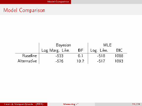
Model Comparison
Bayesian MLE
Log Marg. Like. BF Log. Like. BIC
Baseline -533 0.1 -518 1088
Alternative -526 10.2 -517 1093
Lewis & Vazquez-Grande (FRB) Measuring r∗ 21 / 24

Discussion Thinking about zt
Connection to Theory
The r∗ equation is a linearized euler equation, we can denote the
stochastic discount factor (SDF) by S :
e−r∗t = Et [St+1]
Consider an SDF that di�ers from that of log-utility by an extra term
(Z ) as in Campbell and Cochrane, Epstein-Zin, etc. Then we have
r∗t = log Et
[Ct+1
CtZt+1
]= log Et
[egt+1+zt+1
]≈ Et [gt+1 + zt+1]
zt can be interpreted as an asset pricing term that measures the
separation from log-utility of the SDF. We can give z this �headwinds�
interpretation.
Lewis & Vazquez-Grande (FRB) Measuring r∗ 22 / 24

Discussion Thinking about zt
Headwinds
Frequently, �headwinds� are cited as a reason for why the level of r∗ is
still so low.
�...lingering sense of caution on the part of households and businessesin the wake of the trauma of the Great Recession.� (Yellen, 3/3/17)
zt is the �special sauce� (Williams, 2015 Brookings), it is all the thingsthat are not economic growth.
There is nothing that says the components have to be stationary orpersistent.In the current version of the model, there is no data speci�cally aimedat estimating zt .zt soaks up the variation in the rate gap that doesn't appear to belinked to growth.Headwinds seem like they should be temporary
Lewis & Vazquez-Grande (FRB) Measuring r∗ 23 / 24
Conclusion
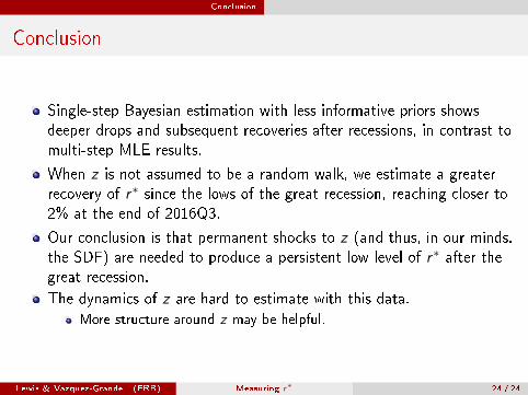
Conclusion
Single-step Bayesian estimation with less informative priors shows
deeper drops and subsequent recoveries after recessions, in contrast to
multi-step MLE results.
When z is not assumed to be a random walk, we estimate a greater
recovery of r∗ since the lows of the great recession, reaching closer to
2% at the end of 2016Q3.
Our conclusion is that permanent shocks to z (and thus, in our minds,
the SDF) are needed to produce a persistent low level of r∗ after the
great recession.
The dynamics of z are hard to estimate with this data.
More structure around z may be helpful.
Lewis & Vazquez-Grande (FRB) Measuring r∗ 24 / 24

APPENDIX
Lewis & Vazquez-Grande (FRB) Measuring r∗ 1 / 34
Estimates
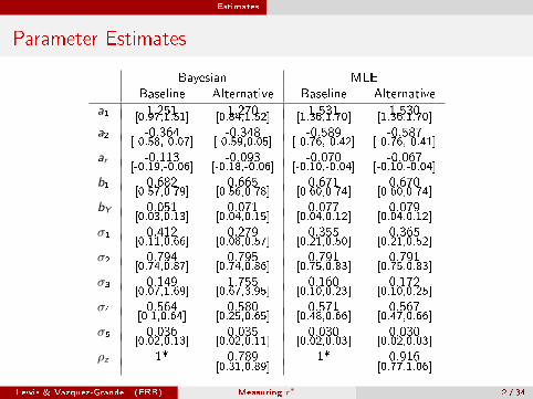
Parameter Estimates
Bayesian MLE
Baseline Alternative Baseline Alternative
a1 1.251 1.270 1.531 1.530[0.97,1.51] [0.84,1.52] [1.36,1.70] [1.36,1.70]
a2 -0.364 -0.348 -0.589 -0.587[-0.58,-0.07] [-0.59,0.05] [-0.76,-0.42] [-0.76,-0.41]
ar -0.113 -0.093 -0.070 -0.067[-0.19,-0.06] [-0.18,-0.06] [-0.10,-0.04] [-0.10,-0.04]
b1 0.682 0.665 0.671 0.670[0.57,0.79] [0.56,0.78] [0.60,0.74] [0.60,0.74]
bY 0.051 0.071 0.077 0.079[0.03,0.13] [0.04,0.15] [0.04,0.12] [0.04,0.12]
σ1 0.412 0.279 0.355 0.365[0.11,0.66] [0.08,0.57] [0.21,0.50] [0.21,0.52]
σ2 0.794 0.795 0.791 0.791[0.74,0.87] [0.74,0.86] [0.75,0.83] [0.75,0.83]
σ3 0.149 1.755 0.160 0.172[0.07,1.69] [0.67,3.95] [0.10,0.23] [0.10,0.25]
σ4 0.564 0.580 0.571 0.567[0.1,0.64] [0.25,0.65] [0.48,0.66] [0.47,0.66]
σ5 0.036 0.035 0.030 0.030[0.02,0.13] [0.02,0.11] [0.02,0.03] [0.02,0.03]
ρz 1* 0.789 1* 0.916[0.31,0.89] [0.77,1.06]
Lewis & Vazquez-Grande (FRB) Measuring r∗ 2 / 34

Laubach-Williams Methodology
Laubach-Williams 3-part Estimation
Step 1 Hold g constant, drop real rate gap from model, then:
- Get estimate of potential output, y∗, compute ∆y∗
- λg is equal to Andrews and Ploberger (1994)
exponential Wald statistic for the test of a structural
break at unknown date in ∆y∗.
Step 2 Impose λg value from Step 1, include real rate gap, but hold
z constant, then:
- Estimate the simpli�ed model
- λz is equal to Wald statistic for the test of a shift in the
intercept of the IS equation.
Step 3 Impose λg from Step 1 and λz from Step 2, and estimate the
remaining parameters by MLE.
Back
Lewis & Vazquez-Grande (FRB) Measuring r∗ 3 / 34

Laubach-Williams Methodology
HLW replication
One-sided Bayesian estimate (blue) and HLW results (red)
back
Lewis & Vazquez-Grande (FRB) Measuring r∗ 4 / 34

Getting Around the �pile-up� problem
DeJong and Whiteman (1993)
Monte Carlo exercise where the true parameter value is 0.85, T = 100
Sample distribution of MLE estimate (left) and posterior distribution (right)
back
Lewis & Vazquez-Grande (FRB) Measuring r∗ 5 / 34

Getting Around the �pile-up� problem
Stock and Watson '98
Our estimation technique does not su�er from the pile-up problem.
To illustrate this: Consider Stock and Watson 1998 local level model of log
GDP growth.
∆yt = βt + ut
βt = βt−1 +λ
Tηt
ut = a1ut−1 + a2ut−2 + a3ut−3 + a4ut−4 + εt
Lewis & Vazquez-Grande (FRB) Measuring r∗ 6 / 34

Getting Around the �pile-up� problem
Replication Stock and Watson 98
0 5 10 15 200
20
40
60
80
100
120
140Histogram of draws of lambda
Lewis & Vazquez-Grande (FRB) Measuring r∗ 7 / 34

Getting Around the �pile-up� problem
Replication Stock and Watson 98
1950 1960 1970 1980 1990 2000 2010 2020 2030-10
-5
0
5
10
15
20dlgdp and beta
back
Lewis & Vazquez-Grande (FRB) Measuring r∗ 8 / 34

Key Posterior Estimates
Key Posterior Estimates From Each Model
Lewis & Vazquez-Grande (FRB) Measuring r∗ 9 / 34

Key Posterior Estimates Model I
Model I: ρg = 1, ρz = 1
Smoothed output gap
Lewis & Vazquez-Grande (FRB) Measuring r∗ 10 / 34

Key Posterior Estimates Model I
Model I: ρg = 1, ρz = 1
Smoothed g path
Lewis & Vazquez-Grande (FRB) Measuring r∗ 11 / 34

Key Posterior Estimates Model I
Model I: ρg = 1, ρz = 1
Smoothed z path
Lewis & Vazquez-Grande (FRB) Measuring r∗ 12 / 34
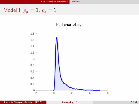
Key Posterior Estimates Model I
Model I: ρg = 1, ρz = 1
Posterior of σr∗
-2 0 2 4 60
0.2
0.4
0.6
0.8
1
1.2
1.4
1.6
1.8
Lewis & Vazquez-Grande (FRB) Measuring r∗ 13 / 34

Key Posterior Estimates Model II
Model II: ρg and µg estimated, ρz = 1
Smoothed output gap
Lewis & Vazquez-Grande (FRB) Measuring r∗ 14 / 34

Key Posterior Estimates Model II
Model II: ρg and µg estimated, ρz = 1
Smoothed g path
Lewis & Vazquez-Grande (FRB) Measuring r∗ 15 / 34

Key Posterior Estimates Model II
Model II: ρg and µg estimated, ρz = 1
Smoothed z path
Lewis & Vazquez-Grande (FRB) Measuring r∗ 16 / 34

Key Posterior Estimates Model II
Model II: ρg and µg estimated, ρz = 1
Posterior of σr∗
-2 0 2 4 60
0.2
0.4
0.6
0.8
1
1.2
1.4
Lewis & Vazquez-Grande (FRB) Measuring r∗ 17 / 34

Key Posterior Estimates Model II
Model II: ρg and µg estimated, ρz = 1
Posterior of ρg
-0.5 0 0.5 1 1.50
0.5
1
1.5
2
2.5
3
3.5
Lewis & Vazquez-Grande (FRB) Measuring r∗ 18 / 34

Key Posterior Estimates Model II
Model II: ρg and µg estimated, ρz = 1
Posterior of µg (Quarterly)
0 0.5 1 1.50
0.5
1
1.5
2
2.5
3
3.5
4
4.5
Lewis & Vazquez-Grande (FRB) Measuring r∗ 19 / 34

Key Posterior Estimates Model III
Model III: ρg = 1, ρz estimated
Smoothed output gap
Lewis & Vazquez-Grande (FRB) Measuring r∗ 20 / 34

Key Posterior Estimates Model III
Model III: ρg = 1, ρz estimated
Smoothed g path
Lewis & Vazquez-Grande (FRB) Measuring r∗ 21 / 34

Key Posterior Estimates Model III
Model III: ρg = 1, ρz estimated
Smoothed z path
Lewis & Vazquez-Grande (FRB) Measuring r∗ 22 / 34

Key Posterior Estimates Model III
Model III: ρg = 1, ρz estimated
Posterior of σr∗
-2 0 2 4 60
0.05
0.1
0.15
0.2
0.25
0.3
0.35
0.4
Lewis & Vazquez-Grande (FRB) Measuring r∗ 23 / 34

Key Posterior Estimates Model III
Model III: ρg = 1, ρz estimated
Posterior of ρz
-0.5 0 0.5 1 1.50
0.5
1
1.5
2
2.5
Lewis & Vazquez-Grande (FRB) Measuring r∗ 24 / 34

Key Posterior Estimates Model IV
Model IV: ρg , µg and ρz estimated
Smoothed output gap
Lewis & Vazquez-Grande (FRB) Measuring r∗ 25 / 34

Key Posterior Estimates Model IV
Model IV: ρg , µg and ρz estimated
Smoothed g path
Lewis & Vazquez-Grande (FRB) Measuring r∗ 26 / 34

Key Posterior Estimates Model IV
Model IV: ρg , µg and ρz estimated
Smoothed z path
Lewis & Vazquez-Grande (FRB) Measuring r∗ 27 / 34

Key Posterior Estimates Model IV
Model IV: ρg , µg and ρz estimated
Posterior of σr∗
-2 0 2 4 60
0.05
0.1
0.15
0.2
0.25
0.3
0.35
Lewis & Vazquez-Grande (FRB) Measuring r∗ 28 / 34

Key Posterior Estimates Model IV
Model IV: ρg , µg and ρz estimated
Posterior of ρg
0 0.2 0.4 0.6 0.8 1 1.20
1
2
3
4
5
6
7
8
Lewis & Vazquez-Grande (FRB) Measuring r∗ 29 / 34

Key Posterior Estimates Model IV
Model IV: ρg , µg and ρz estimated
Posterior of µg (Quarterly)
-1 -0.5 0 0.5 1 1.5 20
0.5
1
1.5
2
2.5
3
3.5
Lewis & Vazquez-Grande (FRB) Measuring r∗ 30 / 34

Key Posterior Estimates Model IV
Model IV: ρg , µg and ρz estimated
Posterior of ρz
-0.5 0 0.5 1 1.50
0.2
0.4
0.6
0.8
1
1.2
1.4
1.6
1.8
Lewis & Vazquez-Grande (FRB) Measuring r∗ 31 / 34

Key Posterior Estimates Other parameters of interest
Model IV: ρg , µg and ρz estimated
Posterior of ar
-0.3 -0.2 -0.1 0 0.10
2
4
6
8
10
12
14
Lewis & Vazquez-Grande (FRB) Measuring r∗ 32 / 34

Key Posterior Estimates Other parameters of interest
Model IV: ρg , µg and ρz estimated
Posterior of bY
0 0.1 0.2 0.3 0.40
2
4
6
8
10
12
Lewis & Vazquez-Grande (FRB) Measuring r∗ 33 / 34

Key Posterior Estimates Other parameters of interest
Model IV: ρg , µg and ρz estimated
Posterior of b1
0.2 0.4 0.6 0.8 10
1
2
3
4
5
6
7
Lewis & Vazquez-Grande (FRB) Measuring r∗ 34 / 34