Embed Size (px)
Citation preview
Measuring Advances in Equality of Opportunity: The
Changing Gender Gap in Educational Attainment in
Canada in the Last Half Century
October 18, 2013
Abstract
The notion of Equality of Opportunity (EO) has pervaded much of economic and so-
cial justice policy over the last half century in conveying a sense of liberation from
the circumstances that constrain an individual’s ability to achieve it, and it has
been a cornerstone of many gender equality programs. However unequivocal pur-
suit of the so called “Luck Egalitarianism” imperative has met with many critics
who question why individuals who are blessed with good circumstances would wish
to be “liberated” from them. This has led to a more qualified pursuit of Equal Op-
portunity which adds an additional proviso − that no circumstance group should be
made worse off by such a policy or decentralized private initiative. Indeed observed
practices, by focusing on the opportunities of the poorly endowed in circumstance,
do accord with such a qualified Equal Opportunity mandate. Here it is contended
that, because of the asymmetric nature of such a policy or initiative, existing empir-
ical techniques will not fully capture the progress made toward an EO goal. Hence
a new technique is introduced and employed in examining progress toward such a
Qualified Equal Opportunity (QEO) Objective in the context of the educational at-
tainments of Canadian males and females born between the 1920s and the 1970s (In
the early part of that century, females did not perform as well as males education-
ally, and were much more constrained by their parental educational circumstance).
A QEO goal is generally found to cohere with the data with females becoming less
attached to their parental educational circumstance, and indeed surpassing males
in their educational attainments.
Key Words: Equality of Opportunity; Overlap Measure
1 Introduction
Atkinson (2012), in his lecture in honour of Amartya Sen, avows that the aim of public
policy reform is ”to remedy injustice rather than characterize perfect justice”. He cites
the introduction to Sen (2009):
In contrast with most modern theories of justice, which concentrate on the just
society, this book is an attempt to investigate realization-based comparisons
that focus on the advancement or retreat of justice.
in pointing out that the aim is progressive reform, rather than transcendental optimality.
Here it is argued that techniques for evaluating such progressive policy reforms should
also be capable of measuring the degree, and significance of such advances, or retreats.
Existing techniques for evaluating the progress of public policy relating to the Equality
of Opportunity (EO) imperative are discussed, and a new approach is introduced.
With roots in recent egalitarian political philosophy1, the Equal Opportunity Impera-
tive sees differential outcomes as ethically acceptable when they are the consequence of
individual choice and action, but not ethically acceptable when they are the consequence
of circumstances beyond the individual’s control. For instance, many affirmative action
type policies, with Equal Opportunity as its objective, have been enacted to address the
extent to which the distribution of individual outcomes is independent of their circum-
stances such as gender and race. Since an individual’s circumstances have to do with
the parents they were blessed with, equal opportunity policies have to address the extent
to which a child’s status is independent of their parents’ status, in order to bring about
independence between the two. In each case, the imperative can be seen to be equalizing
the distributions of people’s capabilitiy to achieve a favourable outcome, given their cir-
cumstance and parental status, seeking a “level playing field” with respect to their given
circumstance. This paper considers the effect of societal equal opportunity aspirations
in the context of the educational attainments of cohorts of Canadian men and women
with respect to their gender, and parental educational circumstances, and in so doing
introduces a new tool for evaluating the extent of equality of opportunity.
The equal opportunity imperative has provoked considerable empirical interest in the
extent of generational mobility (or the degree to which a child’s parental circumstance
conditions his/her outcomes). However, systematically low mobility estimates (i.e. high
1See Arneson (1989), Cohen (1989), Dworkin (1981a), Dworkin (1981b), and Dworkin (2000).
1
correlations between parent and child outcomes, or relatively large diagonal elements in
parent-child transition matrices) over many studies provided little or no support for the
view that the imperative of complete independence of outcome from circumstance has been
achieved2. One rationale for a complete mobility policy objective not being met is that,
from a policy maker’s perspective, other imperatives not necessarily founded upon social
justice sentiments, may be in play. Piketty (2000) noted as much in his interpretation of
the conservative− right wing view that, if generational mobility is low (because of the high
inheritability of ability), and the distortionary costs of welfare redistributions are high, it
is reasonable to argue that low mobility is acceptable.3 Friedman (2005) makes a similar
point in conjecturing (with a considerable amount of supporting evidence) that economic
growth has facilitated the equalizing of opportunities (amongst other improvements in
social justice) in effect allowing the poor to catch up, without disadvantaging the rich.
As noted in Bowles et al. (2005), and Swift (2005), there is inevitable tension between
the public desire for EO in terms of parents not influencing the outcomes of their children,
and the private desire for parents to nurture their offspring. In a democratic society, public
policy will ultimately be a reflection of these competing aspirations. A policy which makes
at least half the inheriting groups worse off than they would have been absent policy, may
not be politically viable (the parents of such groups would almost certainly not vote for
such a policy) so that policy makers responding to the median voter (Downs 1957) or
probabilistic voter (Coughlin 1992) mandates may wish to avoid this part of the package.
Affirmative action policies are very much in this vein since they incorporate normative
objectives that weigh policies in the favour of “poorly” endowed, focusing on improving
the life chances of the “inherited poor”, rather than diminishing the life chances of the
“inherited rich”.4 In effect the policy maker has a second imperative, which is a sort of
2See for example Bowles et al. (2005), and Corak (2004), and references therein3Indeed the pursuit of an equal opportunity goal has not been unequivocal, Anderson (1999), Cavanagh
(2002), Hurley (1993), and Swift (2005) expresses some philosophical reservations, while Jencks and Tach
(2006) question whether an equal opportunity imperative should require the elimination of “..all sources
of economic resemblance between parents and children. Specifically ... (it) ... does not require that society
eliminate the effects of either inherited differences in ability or inherited values regarding the importance
of economic success relative to other goals.”. In a similar vein, Dardanoni et al. (2006) question how
demanding the pursuit of equal opportunity should be in terms of the feasibility of such a pursuit.4As a matter of casual empiricism, equal opportunity programs observed in “Liberal” societies
do seem to be of this flavour. For example, when questioned on the widening gap between the
rich and poor, the British Prime Minister responded that “... the issue is not in fact whether
2
Pareto condition, wherein the lot of the poorly endowed can only be improved without
diminishing the lot of the richly endowed.
With such dual mandates of equal opportunity guided by this Paretian imperative,
a qualified equal opportunity program emerges with asymmetric mobility aspirations for
increasing the mobility of the poorly endowed, and not increasing the mobility of the well
endowed when it involves a loss of their wellbeing. The extent to which these objectives
can be fulfilled is bounded by the capacity in the system to increase average child ability
and outcomes. Such policies and/or decentralised initiatives can no longer be character-
ized as unqualified moves towards the independence of outcomes and circumstances for
all groups. Rather they are equivocal moves, modifying the joint distribution of outcomes
and circumstances differentially toward independence for the poor in circumstance, and
independence for the rich in circumstance only if their wellbeing is not diminished. It
should be noted that interest in the Paretian imperative is not guided by any normative
judgement, but rather by a belief that this may well be how policy and/or initiatives is
formulated in the society being studied.
Attention here is focused on gender educational equality within the Canadian context.
Interest in the gender gap in educational attainment is primarily rooted in the belief that
equal opportunity can best be achieved through education (Roemer 2006), and the fact
that one of the preoccupations of Sen’s considerable body of work on social justice is the
achievement of gender justice (See Nussbaum (2006), Sen (1990), and Sen (1995)). This
could have been achieved quite swiftly by a transfer of resources from the investments
in male human capital to investments in female human capital. Had that been so, an
improvement in the achievements of females accompanied by deterioration in the achieve-
ments of males would have been observed. However it will be shown that, while male
academic achievements did not deteriorate, the narrowing gender gap is characterized by
an increased generational mobility of females relative to males. Furthermore, the source
of this increased mobility was from the daughters of parents with lower educational at-
tainments (which may be construed as “good” since it implies upward mobility), rather
than from the daughters of parents with high educational attainments (which may be
construed as a “bad” since it implies downward mobility, and the attrition of inherited
the very richest person ends up being richer. The issue is the poorest person is given the chance
they don’t otherwise have. The most important thing is to level up, not level down.” Inter-
view with the Prime Minister on BBC News Newsnight on June 4, 2001. Transcript available from
http://news.bbc.co.uk/2/hi/events/newsnight/1372220.stm
3
ability and wellbeing). Indeed, it appears that the increased mobility of females have come
about as a consequence of a reduction in the dependence of their educational outcomes on
those of their mothers, especially at the lower end of the maternal educational attainment
spectrum. However, increasing immobility was observed in the lowest inheritance class.
Since the 1970s, gender equity reform and policy in Canadian school system has largely
been the domain of teachers and their respective associations (Coulter 1996), rather than
a matter of legislation (for example Title IX of the Education Amendment Act in the
United States)5. The Royal Commission on the Status of Women in Canada (1970) listed
education as one of several public policy areas “particularly germane to the status of
women”, and many women’s groups both within and outside of the ambit of the educa-
tion system cited key factors contributing to women’s inequality in Canada as sex-role
stereotyping, the lack of strong female role-models for girls, and inadequate career coun-
seling in schools. Beginning in the 1970’s, a range of lesson plans and units were developed
to assist teachers6. At the same time, other government agencies, institutions, and com-
mercial publishers began producing materials for classroom use. The Ontario Institute
for Studies in Education, for example, compiled “The Women’s Kit” (1974), a collection
of print and audio-visual materials. So began the first stage of curriculum reform.
From the perspective of identification and absolute mobility, a pure equal opportunity
regime would lead to an increase in mobility for all socioeconomic/educational attainment
groups, which in turn implies an ambiguous effect on growth in child educational outcomes.
On the other hand, a qualified equal opportunity regime requires an increase in growth for
the policy to work. Notwithstanding the above difference pertaining to outcome growth,
as will become apparent, identification is primarily from the asymmetry in the attainment
of mobility in terms of educational outcomes. Nonetheless, this asymmetry in mobility,
5Title IX of the Education Amendment Act of 1972 addressed discrimination with respect to gender
in education. Modeled on Title IV an earlier anti-racial discrimination 1964 act, the preamble to Title IX
declared that: “No person in the United States shall, on the basis of sex, be excluded from participation
in, be denied the benefits of, or be subject to discrimination under any educational programs or activity
receiving federal financial assistance ...”.6For example, the British Columbia Teachers’ Federation (BCTF), through its Lesson Aids Service,
published a variety of kits and curriculum packages with titles such as “Women in the Community”,
“Famous Canadian Women”, “Early Canadian Women”, and “From Captivity to Choice: Native Women
in Canadian Literature”. The Ontario Ministry of Education (1977) published a resource guide for
teachers called “Sex-Role Stereotyping and Women’s Studies”, which included units of study, resource
lists, and teaching suggestions for teachers at all grade levels (Coulter 1996).
4
where children of both high and low educational attainment parents have low measures of
mobility as observed in the application, cannot be rationalised by asymmetric borrowing
costs.
There are thus two main contributions in this paper. Firstly, it provides a statistically
flexible measure with which to examine issues regarding mobility, or hypotheses pertaining
to joint density matrices in studies of quality of life. The method is amenable to both
discrete (categorical or ordinal) and continuous variables, and remains viable in many
dimensions. Secondly, it provides an identification strategy for discerning between pure
equality of opportunity versus a qualified version augmented with Pareto concerns, for
differing empirical strategies. These are demonstrated in a simple application within the
Canadian context, examing how equality of opportunity has evolved both across parental
educational groups, and gender.
In section 2, the problems associated with assessing improvements in equality of op-
portunity using conventional methods are examined in the context of both discretely, and
continuously measured indicators. The notion of Qualified Equality of Opportunity is ex-
plored, and a new approach to examining the problem is introduced. These concepts and
their measurement are employed using Statistics Canada’s General Social Survey Cycle
19 (2005) to examine the closing gender gap in educational attainment that occurred in
Canada7 in section 3. Finally some conclusions are drawn in section 4.
7This phenomena has also been observed in the United States, see for example Blau et al. (2006),
Buchmann and Diprete (2006), Dynarski (2007), Goldin et al. (2006), and Jacob (2002).
5
2 Examining Progress toward The Equal Opportu-
nity Imperative
In general, the extent of equality of opportunity has been studied using one or more of
3 different approaches. Generational regressions have been used when the indicators of
interest are continuously measured, to study the degree of dependence of child outcome on
parental outcome8 by examining the proximity to zero of the impact of parental outcomes
on child outcomes, which is estimated by some form of regression technique. When the
variables of interest are discrete or categorical, continuous mobility indices based upon
the relative magnitudes of on and off diagonal elements of the parent-child transition
matrix have been used9 to reflect, to varying degrees, the extent to which the underlying
variables are independent. With complete equality of opportunity, the columns of the
transition matrix would be identical (corresponding to independence between parent and
child outcomes), while with complete dependence, the transition matrix would be the
identity matrix. In essence this approach formulates functions of the elements of the
matrix which measure the extent to which the matrix is not supermodular (see Douglas
et al. (1990), and Shaked and Shanthikumar (2007)). Recently an approach equivalent to
comparing the distributions of the outcomes of children from different parental classes for
the absence of stochastic dominance relationships between the different inheriting group
distributions (LeFranc et al. 2008, 2009) has been suggested.
In the following it will be argued that changes in the coefficient on the parental out-
come in a generational regression or changes in the mobility index prompted by changes in
the relative magnitudes of on and off diagonal elements of a transition matrix will not ad-
equately reflect the asymmetric nature, and hence success or failure, of equal opportunity
policies, especially if they are qualified policies. However while the stochastic dominance
approach will identify the lack of equality of opportunity, unfortunately it does not yield
a statistic which will indicate the degree of change or progress toward equality of oppor-
tunity. To see why this is, and understand why the evaluation of the progress that has
been made, requires rethinking of current empirical approaches to equality of opportunity
8Behrman and Taubman (1990), Solon (1992), Mulligan (1999), Corak and Heisz (1999), Couch and
Lillard (2004), Grawe (2004), and Bratsberg et al. (2007) all being examples.9Bartholemew (1982), Blanden et al. (2004), Chakravarty (1995), Dearden et al. (1997), Hart (1983),
Maasoumi (1986), Maasoumi (1986), Prais (1955), Shorrocks (1978), and Van de Gaer et al. (2001) have
all produced mobility indices many of which are discussed in Maasoumi (1996).
6
measurement, the structure of the equality of opportunity problem, the logic of a quali-
fied equality of opportunity program, and its empirical implications. Broadly speaking, if
there is insufficient capacity in the system to elevate the overall average ability of children,
a pure equality of opportunity policy would inevitably result in the outcomes of children
in some inheritance classes improving at the expense of a deterioration of outcomes of
children in other inheritance classes. If the parent-child outcome relationship is monotonic
and positive (as is usually the case) this means that the outcomes of children with poor
parental endowments will only advance at the expense of the outcomes of richly endowed
children. Such a policy may not be politically viable in a democratic system, since the
interest of the median voters and their inheritors will prevail. Nonetheless, growth in
capacity circumvents this problem, and facilitates a Qualified Equality of Opportunity
policy.
2.1 Qualified Equal Opportunity when Variables are Discrete
When the variable of interest is discrete (for example educational or socioeconomic status),
transition matrix techniques are commonly employed. To illustrate matters in the context
of a transition matrix approach (typically used when outcome measures are discrete),
suppose there are 4 educational categories, that could be attained by both parents and
children, named 1, 2, 3 and 4 which are ordered by their number so 4 is higher than
3 etc.(the model can be generalized to any and different numbers of characteristic, for
both parents and children). Let the transition structure be one where the vector of
parental education outcomes, [1, 2, 3, 4], transit to a vector of child outcomes, [1, 2, 3, 4].
Let the corresponding parent and child outcome probability vectors be [p1, p2, p3, p4] and
[c1, c2, c3, c4] respectively, such that pk = Pr(k) for parents, and ci = Pr(i) for children.
Let J be the matrix of joint probabilities where a typical element ji,k = Pr(i, k) is the
probability of observing a parent-child pairing (i, k), thus:
J =
j1,1 j1,2 j1,3 j1,4
j2,1 j2,2 j2,3 j2,4
j3,1 j3,2 j3,3 j3,4
j4,1 j4,2 j4,3 j4,4
Note that pk =
4∑i=1
ji,k , ci =4∑
k=1
ji,k, and that4∑i=1
ici =4∑i=1
i4∑
k=1
ji,k ≤ µ is a constraint
on average child attainment. Let P = dg(p) (dg being the diagonal operator which
7
converts the vector into a diagonal matrix), then the conventional transition matrix T
that is used for mobility indices can be written as T = JP−1, whose (i, k)th element is
ti,k = Pr(i|k) = ji,k/pk, and yields the child’s education class vector c from the equation
c = Tp (Noting that P−1p = 1, where 1 is vector of ones). In a full equal opportunity
environment, parent and child outcomes will be independent, and the corresponding joint
probability matrix JI = cp′, so that the equal opportunity transition matrix TI will
have common columns c, implying the same conditional density of child outcomes in each
parental category.
A pure equal opportunity program concerned solely with bringing about the indepen-
dence of a child’s outcome from its parents’ outcome shifts any joint density J towards
JI .10 A move toward JI that obeys the average child outcome constraint noted above,
implies that4∑i=1
i4∑
k=1
(jIi,k − ji,k) ≤ 0, and will inevitably make the children of one parental
education group worse off, while making the children of another better off. To see this, first
suppose the population’s joint density matrix exhibits some dependence so that J 6= JI .
Consider the parental socioeconomic group denoted by the index k = 1. Let the nature
of dependence be supermodular such that j1,1 ≥ j2,1 ≥ j3,1 ≥ j4,1. In other words, child
outcomes of the lowest socioeconomic group are positively correlated with their parent’s
socioeconomic status, and the relationship is monotonic so that outcomes of higher en-
dowed children weakly dominate outcomes of lower endowed children. Suppose the move
towards independence shifts the attainment of children in parental group 1 towards higher
attainment. Then by definition j1,1 > jI1,1 = c1p1, and for parental socioeconomic group
1, the following must be true,
m∑i=1
jIi,1 ≤m∑i=1
ji,1
⇒m∑i=1
(jIi,1 − ji,1
)≤ 0 (1)
where m ∈ {1, 2, 3, 4}. In other words, inequality (1) says that a shift towards indepen-
dence leads to a stochastically dominant shift for children of parental socioeconomic group
1. However, the average child attainment constraint implies that j1,k < jI1,k = c1pk, for
10This is the same interpretation as that in Van de Gaer et al. (2001) since with the independence
structure, the probability of attaining an outcome is the same for all children regardless of their parent’s
educational status. The sole difference being the emphasis on joint density here versus the transition
matrix in Van de Gaer et al. (2001).
8
some k ∈ {2, 3, 4}, which in turn means that,
m∑i=1
jIi,k ≥m∑i=1
ji,k
⇒m∑i=1
(jIi,k − ji,k
)≥ 0 (2)
where m ∈ {1, 2, 3, 4}. Inequality (2) then says that for the higher parental group, such a
policy would lead to a stochastically dominated shift. Thus a concommitant of the shift
towards independence without any qualifying conditions on policy, is that the outcomes
of children of higher socioeconomic status parents are necessarily diminished in order that
children of low economic status are advanced. This will always happen unless there is
some potential in the system for average child outcomes to grow. Indeed without any
potential for growth in child outcomes, any qualified policy which at least preserves the
outcomes of all children is not feasible. It is easily demonstrated in the context of this
simple structure that, when there is a possibility for growth in average child outcomes,
stochastically dominant shifts for the poorly parentally endowed children without con-
commitant stochastically dominated shifts for the parentally well endowed are feasible.11
For this reason, progress away from a supermodular transition matrix will not be uniform,
and thus not necessarily detectable with such transition matrix based mobility indices.
For example, some indices computes the magnitude of the diagonal or determinant of T,
whereas movements away from supermudularity can be contrived, which do not affect val-
ues on the diagonal, or the determinant of T. A bigger problem with these techniques is
that when measured child and parent characteristics are not the same, the transition ap-
proach is generally not viable. All of which makes rendering inferences about the progress
of equality of opportunity programs very difficult.
2.2 Qualified Equal Opportunity when Variables are Continuous
When the variable of interest is continuous (for example incomes), equality of opportunity
has frequently been examined via the regression coefficient (β) of a child’s characteristic
when adult (y ∈ Y ) on the corresponding parental characteristic (x ∈ X).
y = α + βx+ γx2 + ε
11Since this will be demonstrated in the following continuous case, it will not be reported here, but is
available from the authors on request.
9
where ε is the population error term. The literature building upon Becker and Tomes
(1979) created a rich class of models highlighting the forces that determined the value of β
(with γ set to 0), which is interpreted as a mobility index, where it inferred mobility (equal
opportunity) as β → 0, and immobility (unequal opportunity) as β → 1. Since Atkinson
(1983) there has been interest in the nonlinearity of generational income elasticity (γ < 0)
or asymmetry of mobility, largely stimulated by the Becker and Tomes (1986) conjecture
that parent-child outcome relationships are concave due to asymmetries in borrowing
constraints. It is worth examining whether qualified equal opportunity policies could
affect the structure of the parent-child relationship, within the context of a generational
regression.
In this continuous paradigm, the policy maker’s dilemma can be illustrated as follows.
Suppose an initial pre-policy state, with parental outcome x ∈ X is distributed with
density f(x), and c.d.f. F (x), with E(x) = µ, V(x) = σ2, and child outcome when adult
is given by:
y = (1− ξ)x+ ξe (3)
where 0 ≤ ξ ≤ 1, and e is distributed as g(e), where g(x) = f(x) for all x, and h(x, e) =
f(x)g(e) (That is to say x and e are identically but independently distributed). So
that Immobility (Unequal Opportunity) implies ξ = 0, when child outcomes are entirely
determined by their parental circumstances, and Mobility (Equal Opportunity) implies
ξ = 1 where child outcomes are entirely determined by luck. Then E(y) = µ (implying
that average ability is constant, so that there is no growth between generations in this
society), and V(y) = (1 + 2ξ(ξ − 1))σ2 for all ξ ∈ [0, 1]. For convenience, let f(x) ∼N(µ, σ2), and note that:
f(y|x) ∼ N((1− ξ)x+ ξµ, ξ2σ2
)for ξ > 0, which accords with the constraint that E(y) ≤ µ. Thus in the pre-policy state,
∂E(y|x)
∂x= (1− ξ) (4)
∂V(y|x)
∂x= 0 (5)
Implying that the intergenerational relationship is linear, and constant across socioeco-
nomic groups, and the relationship is homoskedastic, much like the assumptions underly-
ing the generational regressions commonly found in the literature.
10
Let Φ(.) and φ(.) denote the standard normal c.d.f. and p.d.f. respectively, then for
all ξ < 1, children with parental outcome x∗ have a distribution of outcomes that first
order dominate those of children with parental outcome x∗∗ when x∗ > x∗∗, since for all
y,
F (y|x∗) = Φ
(Y − ((1− ξ)x∗ + ξµ)
ξσ
)≤ Φ
(Y − ((1− ξ)x∗∗ + ξµ)
ξσ
)= F (y|x∗∗)
with strict inequality holding for some Y . Essentially well endowed children are better
off than poorly endowed children except under perfect mobility (ξ = 1). This is what in
effect motivates the stochastic dominance approach to examining equality of opportunity
(LeFranc et al. 2008, 2009) since it seeks to see whether or not the above inequality holds
for any pairs x∗, and x∗∗.
Pure EO policies attempt to increase ξ uniformly across x ∈ X. Consider the marginal
effect of an increase in ξ on the probability that a child’s outcome is less than Y given
parental outcome x∗:
∂ Pr(y < Y |x∗)∂ξ
=∂F (Y |x∗)
∂ξ
=
∂Φ
(Y−E(y|x∗)√
V(y|x∗)
)∂ξ
= φ
(Y − E(y|x∗)√
V(y|x∗)
) ∂ Y−E(y|x∗)√V(y|x∗)
∂ξ
= φ
(Y − E(y|x∗)√
V(y|x∗)
)(x∗ − Yλ2σ
)That is the marginal effect on child outcome of this policy is positive for x∗ > Y , and
negative for x∗ < Y . Thus, ∂ Pr(y<Y |x∗)∂ξ
≤ 0 as x∗ ≤ Y , and ∂ Pr(y<Y |x∗)∂ξ
> 0 as x∗ > Y .
Hence, Fpost(y|x∗)−Fpre(y|x∗) ≥ 0 for y ≤ x∗, and Fpost(y|x∗)−Fpre(y|x∗) < 0 for y > x∗,
so that the pre- and post-policy change cumulative densities, Fpre and Fpost cross just
once at x∗. Here note that both pre- and post-policy outcome distributions are normally
distributed so:∫ x∗
∞(Fpre(y|x∗)− Fpost(y|x∗)) dy T
∫ ∞x∗
(Fpre(y|x∗)− Fpost(y|x∗)) dy as x∗ T E(Y )
11
which means that pre-policy outcomes second order dominate post policy outcomes for
high (above average) parental groups so that average child outcomes diminish for these
groups, whereas post-policy outcomes second order dominate pre-policy outcomes in the
counter cumulative density12 sense for low (below average) parental groups, so that average
child outcomes increase for these groups. If, in this very stylized symmetric world, parents
vote selfishly in the interests of their children, probabilistic or median voter models would
predict a tie between pro EO policy (below median parents), and status quo (above median
parents) voters (the median voter would be indifferent between the two states), and the
policy would face considerable electoral uncertainty.
Consider now a Qualified Equal Opportunity policy where the policy maker is inclined
to increase ξ more for children from lower socioeconomic status families, and less for
those from higher socioeconomic status families (and most importantly it has the growth
capacity to do so), so that ξ now becomes a linear decreasing function of x with ξ′(x) < 0,
0 < ξ(x) ≤ 1 (ξ′′(x) = 0 is assumed for simplicity). Denote the density of the child’s
outcome as f q(.), and the distribution as F q(.). It follows that:
f q(y|x) ∼ N((1− ξ(x))x+ ξ(x)µ, ξ(x)2σ2
)It is readily seen that E(Y ) under this qualified conditional distribution is greater than
E(Y ) under the unqualified conditional distribution, so that average child quality has
increased. Obviously the policymaker has the wherewithal to do this, otherwise the policy
is not feasible. In the post-policy state, among families affected by the Qualified Equal
Opportunity policy,
∂E(y|x)
∂x= 1− ξ(x) + ξ′(x)(µ− x) (6)
∂2 E(y|x)
∂x2= −2ξ′(x) + ξ′′(x)(µ− x) = −2ξ′(x) > 0 (7)
First note that the parent-child relationship is no longer constant across socioeconomic
groups, and that E(y|x) is convex in x compared to the linear relationship of equation
12Second order dominance of the counter cumulative density∫ ∞
x
(Fpre(z)− Fpost(z)) dz ≥ 0 ∀x
with strict inequality holding somewhere, is a sufficient condition for Epre(Y ) = Epost(Y ) (Anderson
2004; Levy and Wiener 1998).
12
(4). In addition,
∂V(y|x)
∂x= 2ξ(x)ξ′(x)σ2 < 0 (8)
implying heteroskedasticity that diminishes with x, instead of homoskedasticity of equa-
tion (5). This implies an increased variance for the poorly endowed, which is the primary
measure of the extent to which children of low outcome parents have been released from
their circumstance. In terms of voting behaviour the impact on the status quo group has
been lessened, and that on the pro-policy group increased so that, within the context of a
probabilistic voting model, the electoral uncertainty regarding the policy has diminished.
This would suggest a quantile regression approach (Koenker 2005). Further, due attention
should still be paid to heteroskedasticity in the error process that this structure engen-
ders13 even in a quantile regression approach, which has never, to the authors knowledge,
been applied in this context.
To restate the key insights, the analysis suggests that whatever the initial generational
regression relationship, a qualified equal opportunity program would (1.) convexify (or re-
duce the concavity of) the parent−child dependence structure, and (2.) make increasingly
negative, the relationship between the conditional error heteroskedasticity and parental
socioeconomic status.
2.3 The Overlap Technique
The technique proposed here measures how close the actual joint density of parent-child
outcomes is to one which reflects either independence (EO) or qualified independence
(QEO) in parent-child outcomes. It does so by measuring the degree of overlap of the
two distributions14 The principal benefits of the measure is in its ease of application, its
statistical properties (it is asymptotically Normal when based upon a random sample,
13Unfortunately due to the categorical nature of the data employed here this approach cannot be
explored in what follows14The Overlap Measure proposed in this paper can be adapted to the three conceptions of intergener-
ational mobility, namely movements across groups, an index of equality of opportunity, and an index of
life chances, suggested by Van de Gaer et al. (2001), since each transition matrix has an implied structure
on the joint density matrix, which the empirical joint density can be measured against. Further, the
third mobility measure for Markov chains proposed by Van de Gaer et al. (2001) is related to the Over-
lap measure in the sense that it measures the complement to the overlapping region of the conditional
probabilities.
13
consequently permitting inference), and its amenability to examining both continuous
and discrete variables, and mixtures thereof in multiple dimensions (see Anderson et al.
(2010), Anderson et al. (2012), and Anderson and Hachem (2012) for details). Specifically,
for the empirical application here, the focus is on,
OV =∑i∈I
∑k∈K
min{joi,k, j
ei,k
}(9)
where joi,k is the typical element of Jo or observed joint density matrix, and jei,k the typical
element of Je in the theoretical joint density matrix. Further, the technique is amenable
to examining not only the independence hypothesis, but any conceivable hypothesis. In-
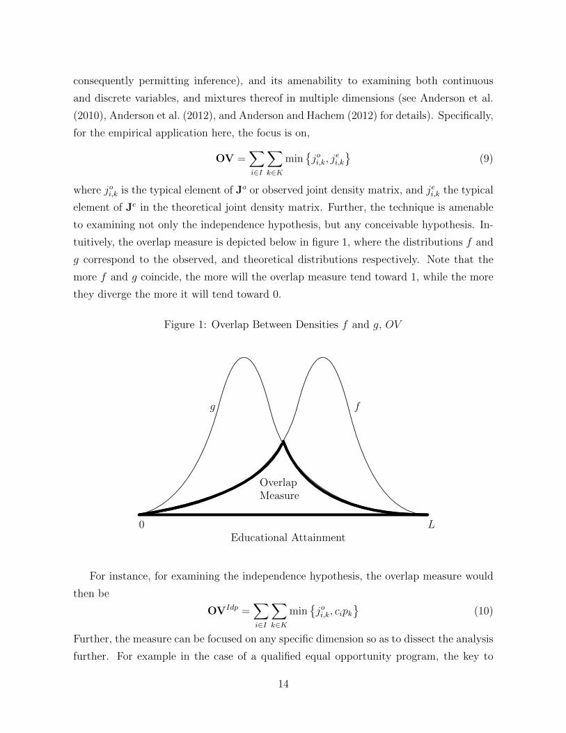
tuitively, the overlap measure is depicted below in figure 1, where the distributions f and
g correspond to the observed, and theoretical distributions respectively. Note that the
more f and g coincide, the more will the overlap measure tend toward 1, while the more
they diverge the more it will tend toward 0.
Figure 1: Overlap Between Densities f and g, OV
0 LEducational Attainment
.............................
............................
............................
............................
............................
..............................
.................................
...................................
......................................
.........................................
...........................................
..............................................
.................................................
.
..................................
..............................
...........................
........................
.....................
..................
...............
............................... ........ ......... ..........
............
...............
..................
.....................
........................
...........................
..............................
..................................
.
........................................
.......................................
.....................................
....................................
...................................
.................................
................................
........................
.........
..........................
........
..............................
.....
....................................
.
......................................
.......................................
.........................................
.......................................... ............................................ ............................................. ..............................................
g
. ..........................................................................................................
..................................................
................................................
..............................................
............................................
..........................................
........................................
......................................
....................................
...................................
....................................
.....................................
......................................
.......................................
........................................
.
..................................
..............................
...........................
........................
.....................
..................
...............
............................... ........ ......... ..........
............
...............
..................
.....................
........................
...........................
..............................
..................................
.
...............................................
.............................................
..........................................
.......................................
.....................................
..................................
...............................
............................
..........................
......................
..
........................
........................
....................... ....................... .......................
f
OverlapMeasurer rrrrrrrrrrrrrrrrrrrr rrrrrrrrrrrrrrrrrrr rrrrrrrrrrrrrrrrrr rrrrrrrrrrrrrrrrr rrrrrrrrrrrrrrrr rrrrrrrrrrrrrrr rrrrrrrrrrrrrr rrrrrrrrrrrrr rrrrrrrrrrrr rrrrrrrrrrr rrrrrrrrrr rrrrrrrrrr rrrrrrrrrr rrrrrrrrrr r rrrrrrrrrrrr rrrrrrrrrrr rrrrrrrrrrr rrrrrrrrrrr rrrrrrrrrr rrrrrrrrrrr rrrrrrrrrrr rrrrrrrrrrrr rrrrrrrrrrrrr rrrrrrrrrrrrr rrrrrrrrrrrrrr rrrrrrrrrrrrrr rrrrrrrrrrrrrrr rrrrrrrrrrrrrrr rrrrrrrrrrrrrrrr rrrrrrrrrrrrrrrrr
For instance, for examining the independence hypothesis, the overlap measure would
then be
OVIdp =∑i∈I
∑k∈K
min{joi,k, cipk
}(10)
Further, the measure can be focused on any specific dimension so as to dissect the analysis
further. For example in the case of a qualified equal opportunity program, the key to
14
identifying if it is benefitting a particular segment of the populace, is through calculating
the overlap measure for each such group.
OVIdpk =
∑i∈I
min
{joi,kpk, ci
}(11)
3 Changes in Gender Gaps, Parental Circumstances
and Educational Attainment in Canada
One profound change in the latter part of the 20th century which exemplifies the equal op-
portunity mandate was the emancipation of women from the household, and the declining
significance of gender concerns in labour markets, thereby raising the incentives for edu-
cational pursuits amongst women (Blau et al. 2006). The advancements made in women’s
status, and wellbeing was possible due to the introduction of the pill, abortion rights and
legislation against gender discrimination in the workplace (Goldin and Katz 2002; Pezzini
2005; Siow 2002). One dimension in which this found expression is in the narrowing of
the gender gap in academic achievement (Dynarski 2007). To study this phenomenon in
light of the hypothesis that equal opportunity policies are qualified in nature, the educa-
tional achievements of successive cohorts of Canadian women conditional on their parents’
are compared both across cohorts, and against their male counterparts. In addition, a
priori under a qualified equal opportunity policy focused on enhancing the wellbeing of
families of lower socioeconomic status as measured by educational attainment, we should
see improvements in the outcomes of their children, regardless of their gender, without
affecting the highest attainment groups. Amalgamating these two concerns, the greatest
improvements in equality of opportunity should be observed in women from the modal,
and lower socioeconomic status families in later cohorts.
3.1 Summary of Data
The data for the empirical analysis on academic achievements of children and their par-
ents in Canada are drawn from Statistics Canada’s General Social Survey Cycle 19
(2005). Educational attainment is indexed from 1 to 5 as follows: 1 for some sec-
ondary/elementary/no education; 2 for high school diploma; 3 for some university; 4
for Diploma/Certificate in a Trade/Technical skill, and 5 for a university degree. This
categorization is for all individuals above the age of 25, including both parents and their
15
children.
Table 1 summarizes the proportion of individuals in each educational attainment cat-
egory, and the corresponding proportion of observations with their parents in those cate-
gories by the individual’s gender and cohort (decade in which they were born). Although
the analysis was performed for all cohorts, the following results reports, and focuses only
on three cohorts, the 70s, 50s, and the 30s and prior cohorts15. Notice first that amongst
individuals born in the 1930s and earlier, the upper attainment levels (in terms of pro-
portions) are dominated by males, but this changes in favour of females in later cohorts,
corresponding with the increased female labour force participation in the post World War
II decades noted previously. Nonetheless, on the aggregate, there is growth in the average
attainment levels amongst the children of each cohort compared to the previous cohorts.
As already noted, an EO policy without growth, such as a pure equal opportunity policy
would engender improvements amongst children of lower socioeconomic status, but a fall
in outcomes amongst children of higher socioeconomic status. Finally, notice the shift in
the modal educational attainment amongst parents from “some/no school” in the pre-30s
cohorts to “high school” by the arrival of the 70s cohort. This has implications regard-
ing the modal group that may be driving the asymmetry in intergenerational mobility
through the five decades as alluded to in the above discussion.
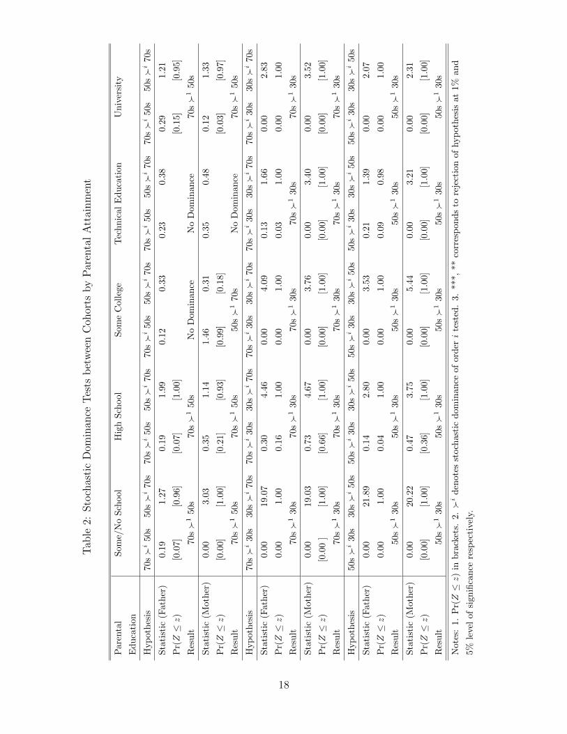
Since a QEO program requires both stochastic dominance criteria, and overall growth
in achievement, these conditions are highlighted in tables 2, and 3. Firstly, table 2 ex-
amines whether through the 5 decades, children of each parental educational group were
made unambiguously worse off or otherwise by employing stochastic dominance tests as
prescribed by Linton et al. (2005) and Dardanoni and Forcina (1998). With the exception
of a few 70s versus 50s comparisons amongst parents with some college and technical ed-
ucation where no dominance relationship was registered, each parental educational group
for each cohort stochastically dominated its preceding cohort unanimously, so improve-
ments in educational outcomes were more or less ubiquitous as expected.
15The discussion that follows extends to the full dataset, and the results in its entirety are available
from the authors upon request.
16
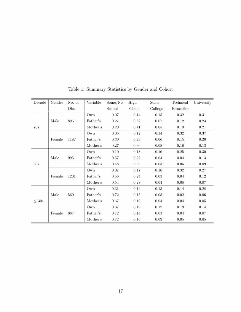
Table 1: Summary Statistics by Gender and Cohort
Decade Gender No. of
Obs.
Variable Some/No
School
High
School
Some
College
Technical
Education
University
Own 0.07 0.14 0.15 0.32 0.31
Male 895 Father’s 0.27 0.32 0.07 0.12 0.23
70s Mother’s 0.20 0.41 0.05 0.13 0.21
Own 0.05 0.12 0.14 0.32 0.37
Female 1187 Father’s 0.30 0.29 0.06 0.15 0.20
Mother’s 0.27 0.36 0.08 0.16 0.13
Own 0.10 0.18 0.16 0.25 0.30
Male 995 Father’s 0.57 0.22 0.04 0.04 0.13
50s Mother’s 0.48 0.35 0.03 0.05 0.09
Own 0.07 0.17 0.16 0.32 0.27
Female 1201 Father’s 0.56 0.24 0.03 0.04 0.12
Mother’s 0.54 0.28 0.04 0.08 0.07
Own 0.31 0.14 0.13 0.14 0.28
Male 569 Father’s 0.72 0.15 0.05 0.02 0.06
≤ 30s Mother’s 0.67 0.19 0.04 0.04 0.05
Own 0.37 0.19 0.12 0.19 0.14
Female 887 Father’s 0.72 0.14 0.03 0.04 0.07
Mother’s 0.72 0.16 0.02 0.05 0.05
17
Tab
le2:
Sto
chas
tic
Dom
inan
ceT
ests
bet
wee
nC
ohor
tsby
Par
enta
lA
ttai
nm
ent
Par
enta
l
Ed
uca
tion
Som
e/N
oS
chool
Hig
hS
chool
Som
eC
oll
ege
Tec
hn
ical
Ed
uca
tion
Un
iver
sity
Hyp
oth
esis
70s�
i50
s50
s�
i70
s70s�
i50s
50s�
i70s
70s�
i50s
50s�
i70s
70s�
i50s
50s�
i70s
70s�
i50s
50s�
i70s
Sta
tist
ic(F
ath
er)
0.19
1.27
0.1
91.9
90.1
20.3
30.2
30.3
80.2
91.2
1
Pr(Z≤z)
[0.0
7][0
.96]
[0.0
7]
[1.0
0]
[0.1
5]
[0.9
5]
Res
ult
70s�
150
s70s�
150s
No
Dom
inan
ceN
oD
om
inan
ce70s�
150s
Sta
tist
ic(M
oth
er)
0.00
3.03
0.3
51.1
41.4
60.3
10.3
50.4
80.1
21.3
3
Pr(Z≤z)
[0.0
0][1
.00]
[0.2
1]
[0.9
3]
[0.9
9]
[0.1
8]
[0.0
3]
[0.9
7]
Res
ult
70s�
150
s70s�
150s
50s�
170s
No
Dom
inan
ce70s�
150s
Hyp
oth
esis
70s�
i30
s30
s�
i70
s70s�
i30s
30s�
i70s
70s�
i30s
30s�
i70s
70s�
i30s
30s�
i70s
70s�
i30s
30s�
i70s
Sta
tist
ic(F
ath
er)
0.00
19.0
70.3
04.4
60.0
04.0
90.1
31.6
60.0
02.8
3
Pr(Z≤z)
0.00
1.00
0.1
61.0
00.0
01.0
00.0
31.0
00.0
01.0
0
Res
ult
70s�
130
s70s�
130s
70s�
130s
70s�
130s
70s�
130s
Sta
tist
ic(M
oth
er)
0.00
19.0
30.7
34.6
70.0
03.7
60.0
03.4
00.0
03.5
2
Pr(Z≤z)
[0.0
0]
[1.0
0][0
.66]
[1.0
0]
[0.0
0]
[1.0
0]
[0.0
0]
[1.0
0]
[0.0
0]
[1.0
0]
Res
ult
70s�
130
s70s�
130s
70s�
130s
70s�
130s
70s�
130s
Hyp
oth
esis
50s�
i30
s30
s�
i50
s50s�
i30s
30s�
i50s
50s�
i30s
30s�
i50s
50s�
i30s
30s�
i50s
50s�
i30s
30s�
i50s
Sta
tist
ic(F
ath
er)
0.00
21.8
90.1
42.8
00.0
03.5
30.2
11.3
90.0
02.0
7
Pr(Z≤z)
0.00
1.00
0.0
41.0
00.0
01.0
00.0
90.9
80.0
01.0
0
Res
ult
50s�
130
s50s�
130s
50s�
130s
50s�
130s
50s�
130s
Sta
tist
ic(M
oth
er)
0.00
20.2
20.4
73.7
50.0
05.4
40.0
03.2
10.0
02.3
1
Pr(Z≤z)
[0.0
0][1
.00]
[0.3
6]
[1.0
0]
[0.0
0]
[1.0
0]
[0.0
0]
[1.0
0]
[0.0
0]
[1.0
0]
Res
ult
50s�
130
s50s�
130s
50s�
130s
50s�
130s
50s�
130s
Not
es:
1.P
r(Z≤z)
inb
rack
ets.
2.�
id
enot
esst
och
ast
icd
om
inan
ceof
ord
eri
test
ed.
3.
***,
**
corr
esp
on
ds
tore
ject
ion
of
hyp
oth
esis
at
1%
an
d
5%le
vel
ofsi
gnifi
can
cere
spec
tivel
y.
18
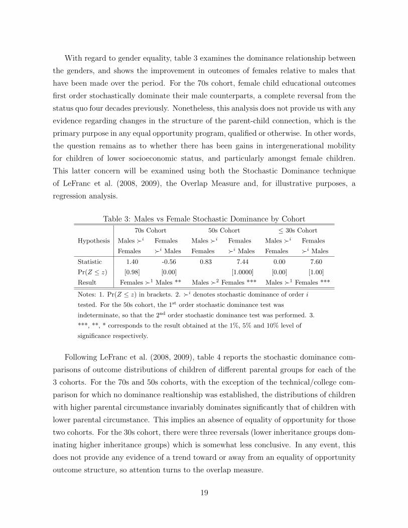
With regard to gender equality, table 3 examines the dominance relationship between
the genders, and shows the improvement in outcomes of females relative to males that
have been made over the period. For the 70s cohort, female child educational outcomes
first order stochastically dominate their male counterparts, a complete reversal from the
status quo four decades previously. Nonetheless, this analysis does not provide us with any
evidence regarding changes in the structure of the parent-child connection, which is the
primary purpose in any equal opportunity program, qualified or otherwise. In other words,
the question remains as to whether there has been gains in intergenerational mobility
for children of lower socioeconomic status, and particularly amongst female children.
This latter concern will be examined using both the Stochastic Dominance technique
of LeFranc et al. (2008, 2009), the Overlap Measure and, for illustrative purposes, a
regression analysis.
Table 3: Males vs Female Stochastic Dominance by Cohort
70s Cohort 50s Cohort ≤ 30s Cohort
Hypothesis Males �i
Females
Females
�i Males
Males �i
Females
Females
�i Males
Males �i
Females
Females
�i Males
Statistic 1.40 -0.56 0.83 7.44 0.00 7.60
Pr(Z ≤ z) [0.98] [0.00] [1.0000] [0.00] [1.00]
Result Females �1 Males ** Males �2 Females *** Males �1 Females ***
Notes: 1. Pr(Z ≤ z) in brackets. 2. �i denotes stochastic dominance of order i
tested. For the 50s cohort, the 1st order stochastic dominance test was
indeterminate, so that the 2nd order stochastic dominance test was performed. 3.
***, **, * corresponds to the result obtained at the 1%, 5% and 10% level of
significance respectively.
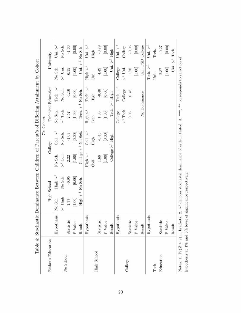
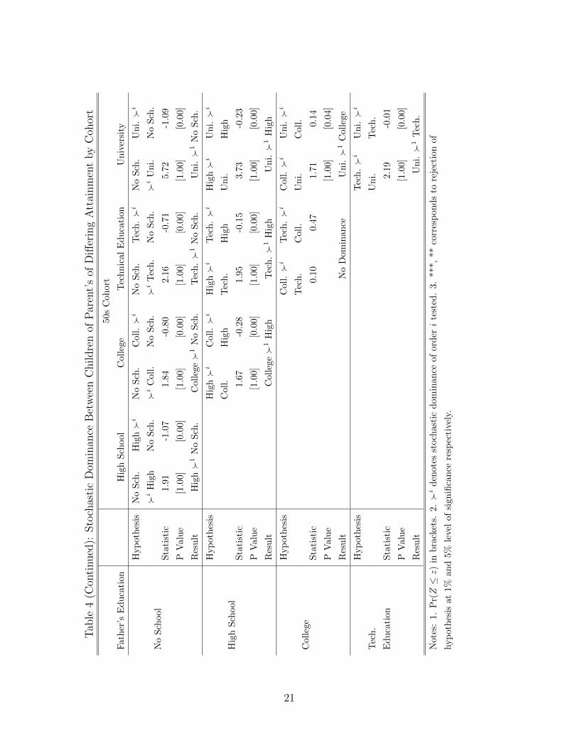
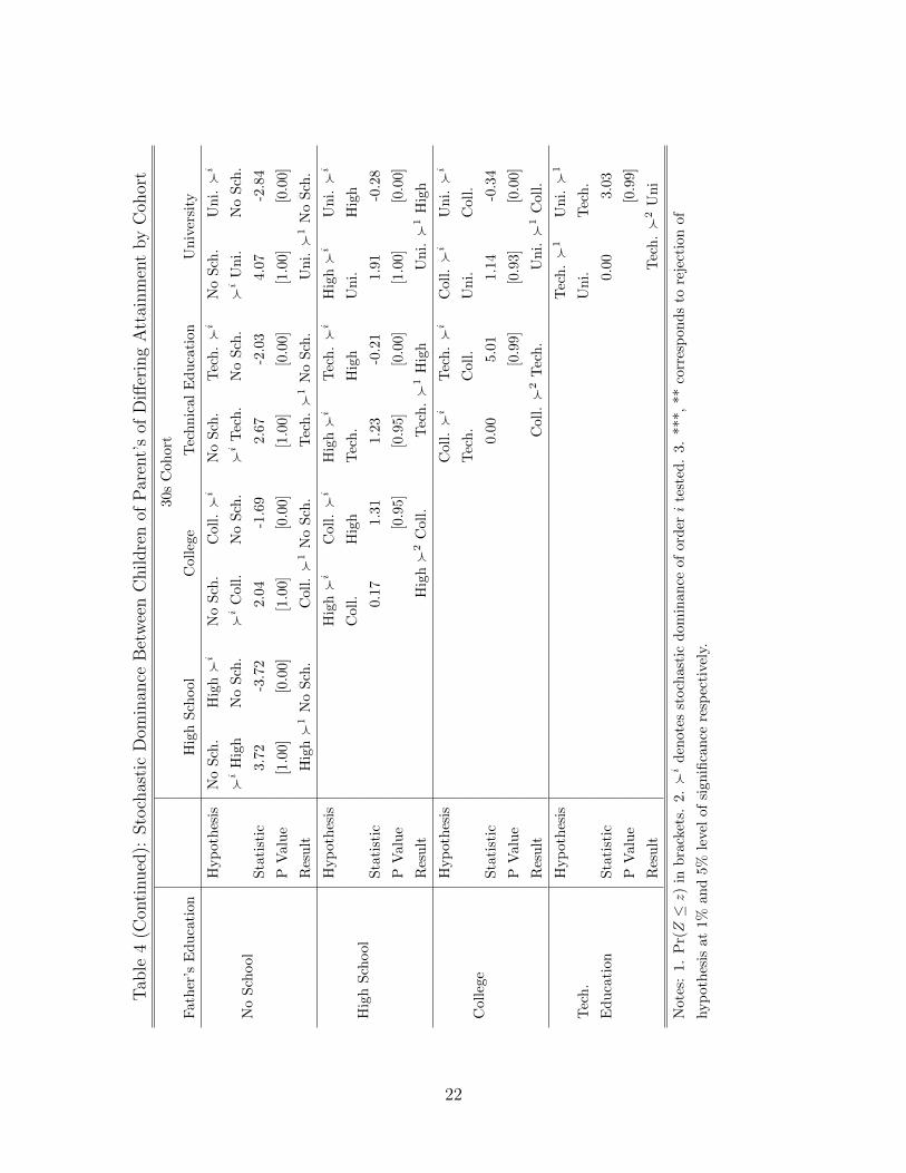
Following LeFranc et al. (2008, 2009), table 4 reports the stochastic dominance com-
parisons of outcome distributions of children of different parental groups for each of the
3 cohorts. For the 70s and 50s cohorts, with the exception of the technical/college com-
parison for which no dominance realtionship was established, the distributions of children
with higher parental circumstance invariably dominates significantly that of children with
lower parental circumstance. This implies an absence of equality of opportunity for those
two cohorts. For the 30s cohort, there were three reversals (lower inheritance groups dom-
inating higher inheritance groups) which is somewhat less conclusive. In any event, this
does not provide any evidence of a trend toward or away from an equality of opportunity
outcome structure, so attention turns to the overlap measure.
19
Tab
le4:
Sto
chas
tic
Dom
inan
ceB
etw
een
Childre
nof
Par
ent’
sof
Diff
erin
gA
ttai
nm
ent
by
Coh
ort
70s
Coh
ort
Fat
her
’sE
du
cati
onH
igh
Sch
ool
Coll
ege
Tec
hn
ical
Ed
uca
tion
Un
iver
sity
No
Sch
ool
Hyp
oth
esis
No
Sch
.
�i
Hig
h
Hig
h�
i
No
Sch
.
No
Sch
.
�i
Coll
.
Coll
.�
i
No
Sch
.
No
Sch
.
�i
Tec
h.
Tec
h.�
i
No
Sch
.
No
Sch
.
�i
Un
i.
Un
i.�
i
No
Sch
.
Sta
tist
ic1.
77
-0.9
52.2
2-1
.03
2.5
7-1
.16
6.1
5-1
.66
PV
alu
e[1
.00]
[0.0
0]
[1.0
0]
[0.0
0]
[1.0
0]
[0.0
0]
[1.0
0]
[0.0
0]
Res
ult
Hig
h�
1N
oS
ch.
Coll
ege�
1N
oS
ch.
Tec
h.�
1N
oS
ch.
Un
i.�
1N
oS
ch
Hig
hS
chool
Hyp
oth
esis
Hig
h�
i
Coll
.
Coll
.�
i
Hig
h
Hig
h�
i
Tec
h.
Tec
h.�
i
Hig
h
Hig
h�
i
Un
i.
Un
i.�
i
Hig
h
Sta
tist
ic1.6
8-0
.45
1.8
6-0
.40
4.4
9-0
.79
PV
alu
e[1
.00]
[0.0
0]
[1.0
0]
[0.0
0]
[1.0
0]
[0.0
0]
Res
ult
Coll
ege�
1H
igh
Tec
h.�
1H
igh
Un
i.�
1H
igh
Col
lege
Hyp
oth
esis
Coll
ege
�i
Tec
h.
Tec
h.�
i
Coll
ege
Coll
ege
�i
Un
i.
Un
i.�
i
Coll
ege
Sta
tist
ic0.0
30.7
81.7
8-0
.05
PV
alu
e[1
.00]
[0.0
0]
Res
ult
No
Dom
inan
ceU
ni.
FS
DC
olleg
e
Tec
h.
Ed
uca
tion
Hyp
oth
esis
Tec
h.�
1
Un
i.
Un
i.�
1
Tec
h.
Sta
tist
ic2.8
7-0
.27
PV
alu
e[1
.00]
[0.0
0]
Res
ult
Un
i.�
1T
ech
Not
es:
1.P
r(Z≤z)
inb
rack
ets.
2.�
id
enote
sst
och
ast
icd
om
inan
ceof
ord
eri
test
ed.
3.
***,
**
corr
esp
on
ds
tore
ject
ion
of
hyp
oth
esis
at1%
and
5%le
vel
ofsi
gnifi
can
cere
spec
tive
ly.
20
Tab
le4
(Con
tinued
):Sto
chas
tic
Dom
inan
ceB
etw
een
Childre
nof
Par
ent’
sof
Diff
erin
gA
ttai
nm
ent
by
Coh
ort
50s
Coh
ort
Fat
her
’sE
du
cati
onH
igh
Sch
ool
Coll
ege
Tec
hn
ical
Ed
uca
tion
Un
iver
sity
No
Sch
ool
Hyp
oth
esis
No
Sch
.
�i
Hig
h
Hig
h�
i
No
Sch
.
No
Sch
.
�i
Coll
.
Coll
.�
i
No
Sch
.
No
Sch
.
�i
Tec
h.
Tec
h.�
i
No
Sch
.
No
Sch
.
�i
Un
i.
Un
i.�
i
No
Sch
.
Sta
tist
ic1.
91
-1.0
71.8
4-0
.80
2.1
6-0
.71
5.7
2-1
.09
PV
alu
e[1
.00]
[0.0
0]
[1.0
0]
[0.0
0]
[1.0
0]
[0.0
0]
[1.0
0]
[0.0
0]
Res
ult
Hig
h�
1N
oS
ch.
Coll
ege�
1N
oS
ch.
Tec
h.�
1N
oS
ch.
Un
i.�
1N
oS
ch.
Hig
hS
chool
Hyp
oth
esis
Hig
h�
i
Coll
.
Coll
.�
i
Hig
h
Hig
h�
i
Tec
h.
Tec
h.�
i
Hig
h
Hig
h�
i
Un
i.
Un
i.�
i
Hig
h
Sta
tist
ic1.6
7-0
.28
1.9
5-0
.15
3.7
3-0
.23
PV
alu
e[1
.00]
[0.0
0]
[1.0
0]
[0.0
0]
[1.0
0]
[0.0
0]
Res
ult
Coll
ege�
1H
igh
Tec
h.�
1H
igh
Un
i.�
1H
igh
Col
lege
Hyp
oth
esis
Coll
.�
i
Tec
h.
Tec
h.�
i
Coll
.
Coll
.�
i
Un
i.
Un
i.�
i
Coll
.
Sta
tist
ic0.1
00.4
71.7
10.1
4
PV
alu
e[1
.00]
[0.0
4]
Res
ult
No
Dom
inan
ceU
ni.�
1C
oll
ege
Tec
h.
Ed
uca
tion
Hyp
oth
esis
Tec
h.�
i
Un
i.
Un
i.�
i
Tec
h.
Sta
tist
ic2.1
9-0
.01
PV
alu
e[1
.00]
[0.0
0]
Res
ult
Un
i.�
1T
ech
.
Not
es:
1.P
r(Z≤z)
inb
rack
ets.
2.�
id
enote
sst
och
ast
icd
om
inan
ceof
ord
eri
test
ed.
3.
***,
**
corr
esp
on
ds
tore
ject
ion
of
hyp
oth
esis
at1%
and
5%le
vel
ofsi
gnifi
can
cere
spec
tive
ly.
21
Tab
le4
(Con
tinued
):Sto
chas
tic
Dom
inan
ceB
etw
een
Childre
nof
Par
ent’
sof
Diff
erin
gA
ttai
nm
ent
by
Coh
ort
30s
Coh
ort
Fat
her
’sE
du
cati
onH
igh
Sch
ool
Coll
ege
Tec
hn
ical
Ed
uca
tion
Un
iver
sity
No
Sch
ool
Hyp
oth
esis
No
Sch
.
�i
Hig
h
Hig
h�
i
No
Sch
.
No
Sch
.
�i
Coll
.
Coll
.�
i
No
Sch
.
No
Sch
.
�i
Tec
h.
Tec
h.�
i
No
Sch
.
No
Sch
.
�i
Un
i.
Un
i.�
i
No
Sch
.
Sta
tist
ic3.
72
-3.7
22.0
4-1
.69
2.6
7-2
.03
4.0
7-2
.84
PV
alu
e[1
.00]
[0.0
0]
[1.0
0]
[0.0
0]
[1.0
0]
[0.0
0]
[1.0
0]
[0.0
0]
Res
ult
Hig
h�
1N
oS
ch.
Coll
.�
1N
oS
ch.
Tec
h.�
1N
oS
ch.
Un
i.�
1N
oS
ch.
Hig
hS
chool
Hyp
oth
esis
Hig
h�
i
Coll
.
Coll
.�
i
Hig
h
Hig
h�
i
Tec
h.
Tec
h.�
i
Hig
h
Hig
h�
i
Un
i.
Un
i.�
i
Hig
h
Sta
tist
ic0.1
71.3
11.2
3-0
.21
1.9
1-0
.28
PV
alu
e[0
.95]
[0.9
5]
[0.0
0]
[1.0
0]
[0.0
0]
Res
ult
Hig
h�
2C
oll
.T
ech
.�
1H
igh
Un
i.�
1H
igh
Col
lege
Hyp
oth
esis
Coll
.�
i
Tec
h.
Tec
h.�
i
Coll
.
Coll
.�
i
Un
i.
Un
i.�
i
Coll
.
Sta
tist
ic0.0
05.0
11.1
4-0
.34
PV
alu
e[0
.99]
[0.9
3]
[0.0
0]
Res
ult
Coll
.�
2T
ech
.U
ni.�
1C
oll
.
Tec
h.
Ed
uca
tion
Hyp
oth
esis
Tec
h.�
1
Un
i.
Un
i.�
1
Tec
h.
Sta
tist
ic0.0
03.0
3
PV
alu
e[0
.99]
Res
ult
Tec
h.�
2U
ni
Not
es:
1.P
r(Z≤z)
inb
rack
ets.
2.�
id
enote
sst
och
ast
icd
om
inan
ceof
ord
eri
test
ed.
3.
***,
**
corr
esp
on
ds
tore
ject
ion
of
hyp
oth
esis
at1%
and
5%le
vel
ofsi
gnifi
can
cere
spec
tive
ly.
22
3.2 Examining Qualified Equal Opportunity using the Overlap
Measure
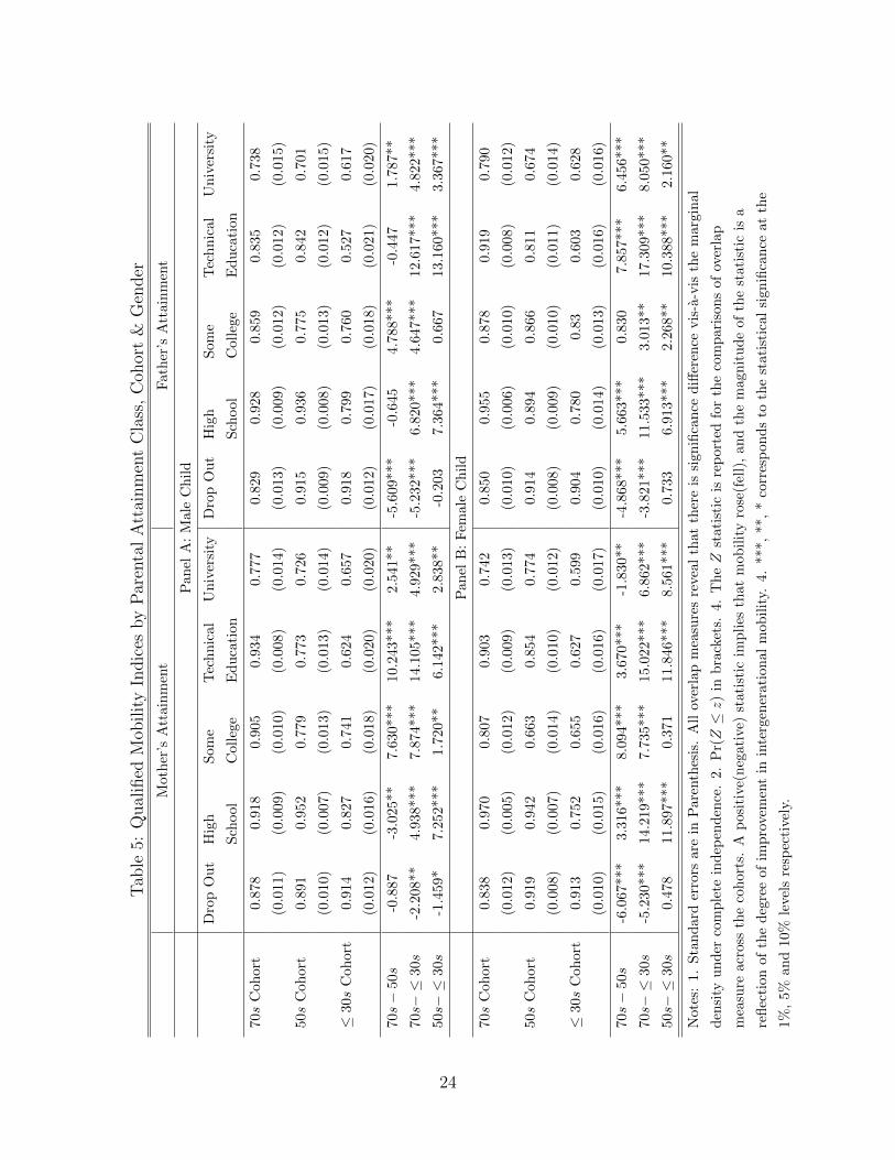
The qualified equal opportunity hypothesis suggests that the conditional density of child
attainment for lower socioeconomic groups should be a closer match to the marginal den-
sity of child attainment relative to the children from higher socioeconomic status groups,
since a qualified policy would leave the latter group relatively untouched. Equation (11)
above provides a test that will be performed, which intuitively measures the degree of
overlap between two densities for each parental socioeconomic status/educational attain-
ment group. In obtaining the measure, all observations were weighted by their individual
weights. If the child’s educational outcome and parental circumstances are independent,
the Overlap measure will record values close to 1 corresponding to equality of opportunity
for that group. To the extent that they are not independent, the statistic will record a
value substantially less than 1 reflecting the greater attachment of a child’s outcome to its
parents. The results of this measure for each parental attainment outcome by the gender
of the children are reported in table 5.
What is immediately striking from table 5 is the ubiquitous trend over the decades
toward greater equality of opportunity amongst children of both genders from families with
parents who have high school, some college, and technical education over the decades, as
reflected in the closer proximity of the overlap measure to 1. Improvements in EO amongst
children of parents of university degrees are somewhat more attenuated, with the overlap
measure remaining significantly lower than for children in the other educational groups.
The gains are particularly impressive for children of parents with education at or above a
high school diploma when compared to the low levels of overlap amongst the generation
in the oldest cohort from the 30s. Due to the asymptotic normality of the measures, the
significance of the improvements can be determined by a standard normal test of their
differences. The value of the statistic informs us of the magnitude of improvement, while
the sign tells us if mobility improved (if positive) or fell (if negative). The magnitude of
these gains are reported in table 5 below the corresponding overlap measures.
23
Tab
le5:
Qual
ified
Mob
ilit
yIn
dic
esby
Par
enta
lA
ttai
nm
ent
Cla
ss,
Coh
ort
&G
ender
Mot
her
’sA
ttain
men
tF
ath
er’s
Att
ain
men
t
Pan
elA
:M
ale
Ch
ild
Dro
pO
ut
Hig
h
Sch
ool
Som
e
Coll
ege
Tec
hn
ical
Ed
uca
tion
Un
iver
sity
Dro
pO
ut
Hig
h
Sch
ool
Som
e
Coll
ege
Tec
hn
ical
Ed
uca
tion
Un
iver
sity
70s
Coh
ort
0.87
80.
918
0.9
05
0.9
34
0.7
77
0.8
29
0.9
28
0.8
59
0.8
35
0.7
38
(0.0
11)
(0.0
09)
(0.0
10)
(0.0
08)
(0.0
14)
(0.0
13)
(0.0
09)
(0.0
12)
(0.0
12)
(0.0
15)
50s
Coh
ort
0.89
10.
952
0.7
79
0.7
73
0.7
26
0.9
15
0.9
36
0.7
75
0.8
42
0.7
01
(0.0
10)
(0.0
07)
(0.0
13)
(0.0
13)
(0.0
14)
(0.0
09)
(0.0
08)
(0.0
13)
(0.0
12)
(0.0
15)
≤30s
Coh
ort
0.91
40.
827
0.7
41
0.6
24
0.6
57
0.9
18
0.7
99
0.7
60
0.5
27
0.6
17
(0.0
12)
(0.0
16)
(0.0
18)
(0.0
20)
(0.0
20)
(0.0
12)
(0.0
17)
(0.0
18)
(0.0
21)
(0.0
20)
70s−
50s
-0.8
87-3
.025
**7.
630***
10.2
43***
2.5
41**
-5.6
09***
-0.6
45
4.7
88***
-0.4
47
1.7
87**
70s−≤
30s
-2.2
08**
4.93
8***
7.874***
14.1
05***
4.9
29***
-5.2
32***
6.8
20***
4.6
47***
12.6
17***
4.8
22***
50s−≤
30s
-1.4
59*
7.25
2***
1.7
20**
6.1
42***
2.8
38**
-0.2
03
7.3
64***
0.6
67
13.1
60***
3.3
67***
Pan
elB
:F
emale
Ch
ild
70s
Coh
ort
0.83
80.
970
0.8
07
0.9
03
0.7
42
0.8
50
0.9
55
0.8
78
0.9
19
0.7
90
(0.0
12)
(0.0
05)
(0.0
12)
(0.0
09)
(0.0
13)
(0.0
10)
(0.0
06)
(0.0
10)
(0.0
08)
(0.0
12)
50s
Coh
ort
0.91
90.
942
0.6
63
0.8
54
0.7
74
0.9
14
0.8
94
0.8
66
0.8
11
0.6
74
(0.0
08)
(0.0
07)
(0.0
14)
(0.0
10)
(0.0
12)
(0.0
08)
(0.0
09)
(0.0
10)
(0.0
11)
(0.0
14)
≤30s
Coh
ort
0.91
30.
752
0.6
55
0.6
27
0.5
99
0.9
04
0.7
80
0.8
30.6
03
0.6
28
(0.0
10)
(0.0
15)
(0.0
16)
(0.0
16)
(0.0
17)
(0.0
10)
(0.0
14)
(0.0
13)
(0.0
16)
(0.0
16)
70s−
50s
-6.0
67**
*3.
316*
**8.
094***
3.6
70***
-1.8
30**
-4.8
68***
5.6
63***
0.8
307.8
57***
6.4
56***
70s−≤
30s
-5.2
30**
*14
.219
***
7.735***
15.0
22***
6.8
62***
-3.8
21***
11.5
33***
3.0
13*
*17.3
09***
8.0
50***
50s−≤
30s
0.47
811
.897
***
0.3
71
11.8
46***
8.5
61***
0.7
33
6.9
13***
2.2
68*
*10.3
88***
2.1
60**
Not
es:
1.S
tan
dar
der
rors
are
inP
aren
thes
is.
All
over
lap
mea
sure
sre
vea
lth
at
ther
eis
sign
ifica
nce
diff
eren
cevis
-a-v
isth
em
arg
inal
den
sity
un
der
com
ple
tein
dep
end
ence
.2.
Pr(Z≤z)
inb
rack
ets.
4.
Th
eZ
stati
stic
isre
port
edfo
rth
eco
mp
ari
son
sof
over
lap
mea
sure
acro
ssth
eco
hor
ts.
Ap
osit
ive(
neg
ati
ve)
stati
stic
imp
lies
that
mob
ilit
yro
se(f
ell)
,an
dth
em
agn
itu
de
ofth
est
ati
stic
isa
refl
ecti
onof
the
deg
ree
ofim
pro
vem
ent
inin
terg
ener
ati
on
al
mob
ilit
y.4.
***,
**,
*co
rres
pon
ds
toth
est
ati
stic
al
sign
ifica
nce
at
the
1%,
5%an
d10
%le
vel
sre
spec
tive
ly.
24
Amongst male children, those from families with parents with education at or greater
than a high school diploma enjoyed significant gains up to the 50s. However, there was
an apparent slow down in the gains in EO amongst the 70s cohort, with some evidence of
children of high school diploma parents suffering a fall. This gain is also apparent amongst
female children, with the evidence here being far stronger, and more consistent through
to the 70s for women of parents with education at and beyond high school. In all of this,
children of parents who had not completed their high school diploma, regardless of gender,
saw a consistent decline in EO, suggesting that EO policies were not effective in elevating
the state of these most disadvantaged children. However it should be noted that the levels
of EO, as evident from the proximity of the overlap measure to 1, has been high amongst
these disadvantaged children. In other words, their social mobility has always been closer
to independence, in stark contrast to children of parents with university education.
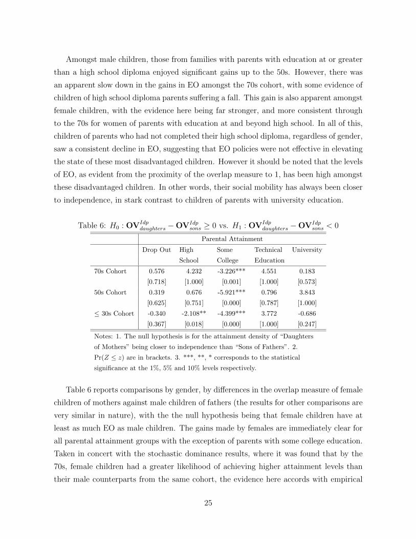
Table 6: H0 : OVIdpdaughters −OVIdp
sons ≥ 0 vs. H1 : OVIdpdaughters −OVIdp
sons < 0
Parental Attainment
Drop Out High
School
Some
College
Technical
Education
University
70s Cohort 0.576 4.232 -3.226*** 4.551 0.183
[0.718] [1.000] [0.001] [1.000] [0.573]
50s Cohort 0.319 0.676 -5.921*** 0.796 3.843
[0.625] [0.751] [0.000] [0.787] [1.000]
≤ 30s Cohort -0.340 -2.108** -4.399*** 3.772 -0.686
[0.367] [0.018] [0.000] [1.000] [0.247]
Notes: 1. The null hypothesis is for the attainment density of “Daughters
of Mothers” being closer to independence than “Sons of Fathers”. 2.
Pr(Z ≤ z) are in brackets. 3. ***, **, * corresponds to the statistical
significance at the 1%, 5% and 10% levels respectively.
Table 6 reports comparisons by gender, by differences in the overlap measure of female
children of mothers against male children of fathers (the results for other comparisons are
very similar in nature), with the the null hypothesis being that female children have at
least as much EO as male children. The gains made by females are immediately clear for
all parental attainment groups with the exception of parents with some college education.
Taken in concert with the stochastic dominance results, where it was found that by the
70s, female children had a greater likelihood of achieving higher attainment levels than
their male counterparts from the same cohort, the evidence here accords with empirical
25
evidence of the narrowing in gender wage gap within the labour market, and the overall
increased liberation of females from their circumstance relative to males.
3.3 The Generational Regression Approach
As noted in the introduction, a qualified equal opportunity program creates nonlinear
effects for differing genders and parental attainment groups, which in turn has direct
implications for regression analysis. To illustrate these effects here in the context of
generational regressions, the model considered is of the form:
yi,k = β0,k + β1,kxi,k + β2,kx2i,k + εi,k (12)
where E(εi,k) = 0 and E(ln ε2i,k) = α0,k+αi,1xi,k where i = {1, 2, ..., nk}, k = {male, female}.As before y corresponds to the child, and x the parent’s outcome (in terms of educational
attainment), and heteroskedasticity is modeled in terms of the log squared error being a
linear function of parental attainment. That is a secondary regression will be performed
on the residuals to examine the changes in variance across the cohorts,
εi,k = α0,k + α1,kxi,k + ηi,k (13)
Note that parent and child variables here are both discrete integer variables which pre-
clude a quantile regression approach, and would usually require some sort of multinomial
technique for analysis since the residuals from regressions which employ them will have
heteroskedastic errors. However the hypotheses considered here are that the regression re-
lationship will become increasingly “convexified” over successive cohort regressions, and
that heteroskedasticity will become increasingly negatively related to parental status,
both of which for simplicity can readily be examined via the characteristics of a simple
regression model with these albeit discrete variables. The results are reported in table 7.
At the outset, observe the positive effect that parental attainment has on child out-
comes, regardless of gender and cohort, from both panels A and B of table 7, with the
effect waning more for male children than female. Adopting the usual interpretation that
proximity of this coefficient to zero reveals proximity to independence, this suggests that
male children made greater gains in mobility. This thus runs counter to the above find-
ings utilizing the overlap measure, where it was found that gains in EO were stronger for
females than they were for males. This suggests limitations in intergenerational mobility
regressions relative to examinations of joint density functions, since the former approach
26
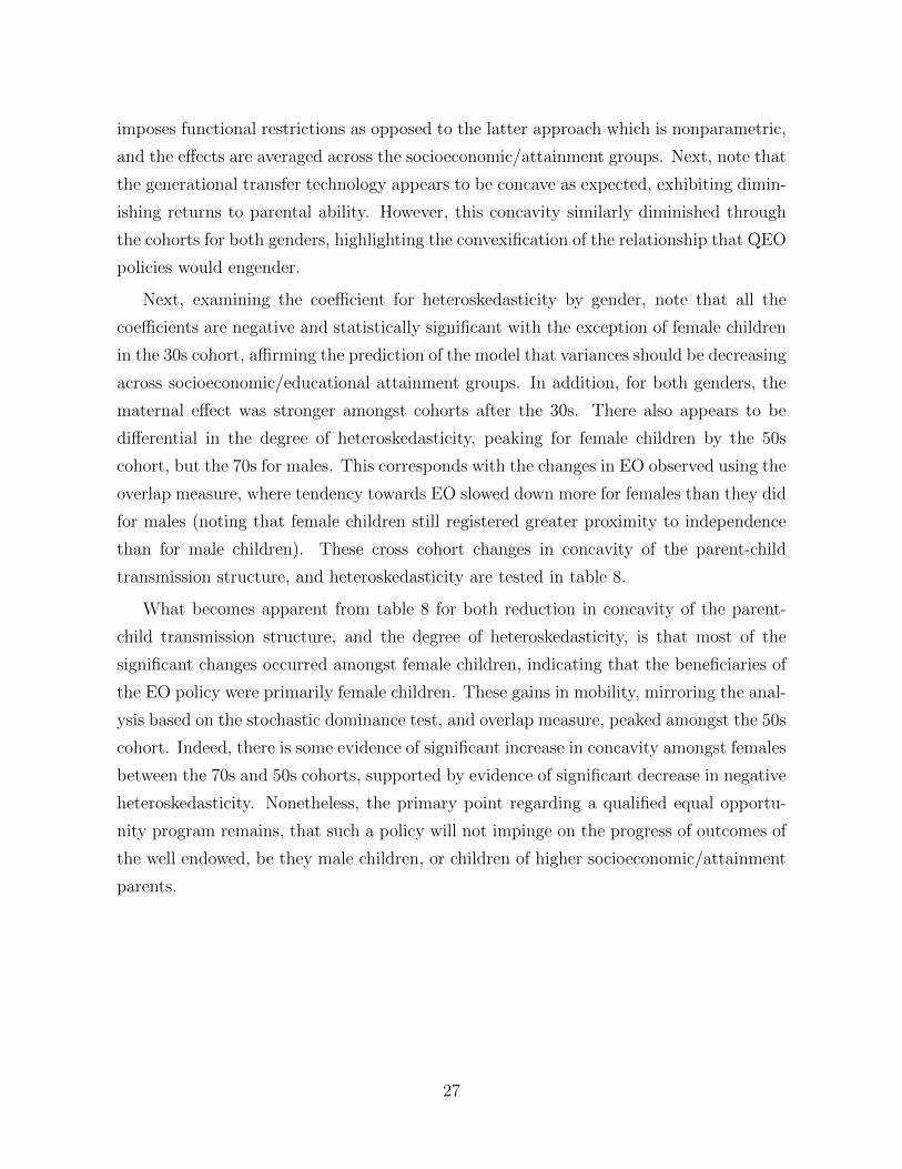
imposes functional restrictions as opposed to the latter approach which is nonparametric,
and the effects are averaged across the socioeconomic/attainment groups. Next, note that
the generational transfer technology appears to be concave as expected, exhibiting dimin-
ishing returns to parental ability. However, this concavity similarly diminished through
the cohorts for both genders, highlighting the convexification of the relationship that QEO
policies would engender.
Next, examining the coefficient for heteroskedasticity by gender, note that all the
coefficients are negative and statistically significant with the exception of female children
in the 30s cohort, affirming the prediction of the model that variances should be decreasing
across socioeconomic/educational attainment groups. In addition, for both genders, the
maternal effect was stronger amongst cohorts after the 30s. There also appears to be
differential in the degree of heteroskedasticity, peaking for female children by the 50s
cohort, but the 70s for males. This corresponds with the changes in EO observed using the
overlap measure, where tendency towards EO slowed down more for females than they did
for males (noting that female children still registered greater proximity to independence
than for male children). These cross cohort changes in concavity of the parent-child
transmission structure, and heteroskedasticity are tested in table 8.
What becomes apparent from table 8 for both reduction in concavity of the parent-
child transmission structure, and the degree of heteroskedasticity, is that most of the
significant changes occurred amongst female children, indicating that the beneficiaries of
the EO policy were primarily female children. These gains in mobility, mirroring the anal-
ysis based on the stochastic dominance test, and overlap measure, peaked amongst the 50s
cohort. Indeed, there is some evidence of significant increase in concavity amongst females
between the 70s and 50s cohorts, supported by evidence of significant decrease in negative
heteroskedasticity. Nonetheless, the primary point regarding a qualified equal opportu-
nity program remains, that such a policy will not impinge on the progress of outcomes of
the well endowed, be they male children, or children of higher socioeconomic/attainment
parents.
27
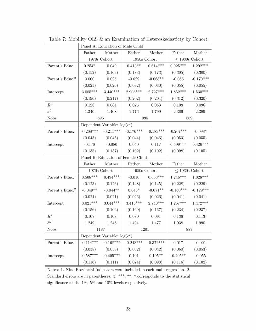
Table 7: Mobility OLS & an Examination of Heteroskedasticty by Cohort
Panel A: Education of Male Child
Father Mother Father Mother Father Mother
1970s Cohort 1950s Cohort ≤ 1930s Cohort
Parent’s Educ. 0.254* 0.049 0.413** 0.614*** 0.925*** 1.292***
(0.152) (0.163) (0.183) (0.173) (0.305) (0.300)
Parent’s Educ.2 0.000 0.025 -0.029 -0.068** -0.085 -0.170***
(0.025) (0.026) (0.032) (0.030) (0.055) (0.055)
Intercept 3.085*** 3.440*** 2.903*** 2.727*** 1.852*** 1.530***
(0.196) (0.217) (0.202) (0.204) (0.312) (0.320)
R2 0.128 0.084 0.075 0.063 0.108 0.096
σ2 1.340 1.408 1.776 1.799 2.366 2.399
Nobs 895 995 569
Dependent Variable: log(ε2)
Parent’s Educ. -0.208*** -0.211*** -0.176*** -0.183*** -0.207*** -0.098*
(0.043) (0.045) (0.044) (0.046) (0.053) (0.055)
Intercept -0.178 -0.080 0.040 0.117 0.599*** 0.426***
(0.135) (0.137) (0.102) (0.102) (0.098) (0.105)
Panel B: Education of Female Child
Father Mother Father Mother Father Mother
1970s Cohort 1950s Cohort ≤ 1930s Cohort
Parent’s Educ. 0.508*** 0.494*** -0.010 0.658*** 1.246*** 1.028***
(0.123) (0.126) (0.148) (0.145) (0.228) (0.229)
Parent’s Educ.2 -0.049** -0.044** 0.043* -0.071** -0.160*** -0.129***
(0.021) (0.021) (0.026) (0.026) (0.041) (0.041)
Intercept 3.021*** 3.044*** 3.415*** 2.740*** 1.257*** 1.472***
(0.156) (0.162) (0.169) (0.167) (0.234) (0.237)
R2 0.107 0.108 0.080 0.091 0.136 0.113
σ2 1.249 1.248 1.494 1.477 1.938 1.990
Nobs 1187 1201 887
Dependent Variable: log(ε2)
Parent’s Educ. -0.114*** -0.168*** -0.248*** -0.372*** 0.017 -0.001
(0.038) (0.038) (0.032) (0.042) (0.060) (0.053)
Intercept -0.587*** -0.405*** 0.101 0.195** -0.205** -0.055
(0.116) (0.111) (0.074) (0.093) (0.116) (0.102)
Notes: 1. Nine Provincial Indicators were included in each main regression. 2.
Standard errors are in parentheses. 3. ***, **, * corresponds to the statistical
significance at the 1%, 5% and 10% levels respectively.
28
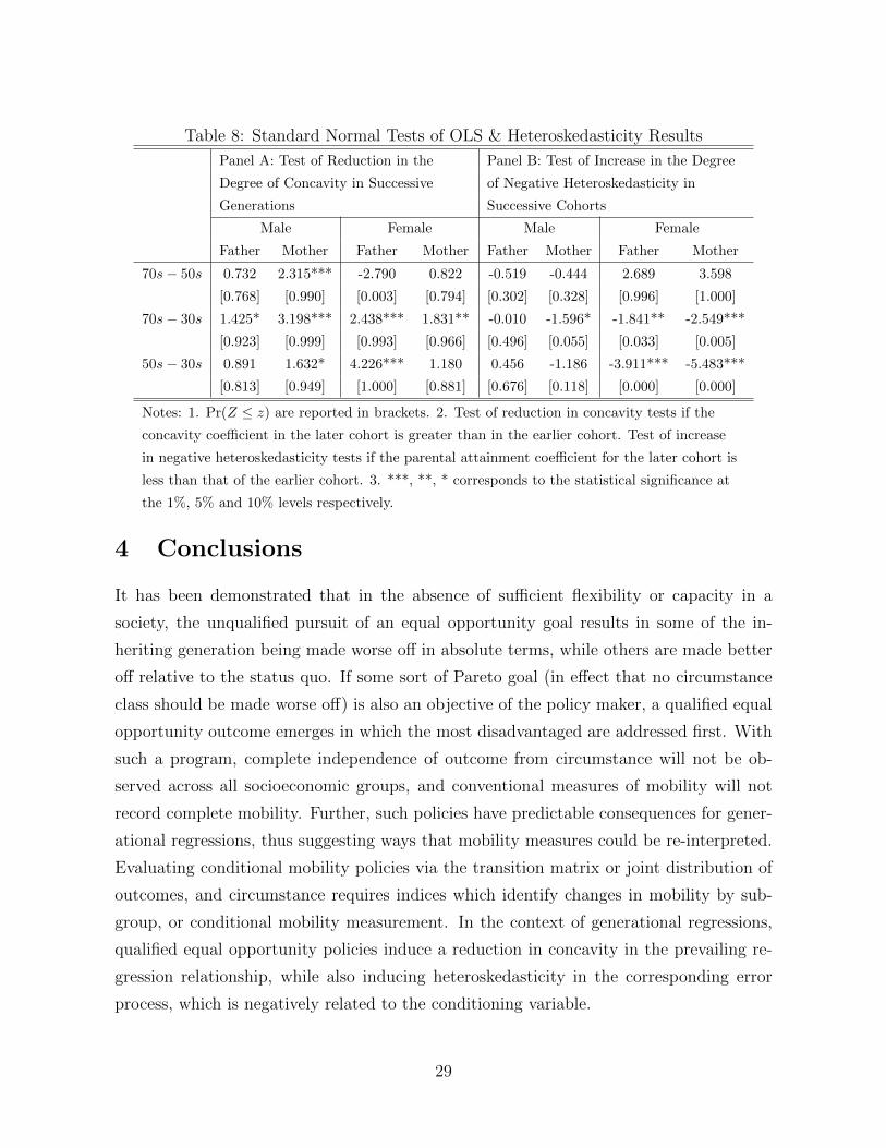
Table 8: Standard Normal Tests of OLS & Heteroskedasticity Results
Panel A: Test of Reduction in the
Degree of Concavity in Successive
Generations
Panel B: Test of Increase in the Degree
of Negative Heteroskedasticity in
Successive Cohorts
Male Female Male Female
Father Mother Father Mother Father Mother Father Mother
70s− 50s 0.732 2.315*** -2.790 0.822 -0.519 -0.444 2.689 3.598
[0.768] [0.990] [0.003] [0.794] [0.302] [0.328] [0.996] [1.000]
70s− 30s 1.425* 3.198*** 2.438*** 1.831** -0.010 -1.596* -1.841** -2.549***
[0.923] [0.999] [0.993] [0.966] [0.496] [0.055] [0.033] [0.005]
50s− 30s 0.891 1.632* 4.226*** 1.180 0.456 -1.186 -3.911*** -5.483***
[0.813] [0.949] [1.000] [0.881] [0.676] [0.118] [0.000] [0.000]
Notes: 1. Pr(Z ≤ z) are reported in brackets. 2. Test of reduction in concavity tests if the
concavity coefficient in the later cohort is greater than in the earlier cohort. Test of increase
in negative heteroskedasticity tests if the parental attainment coefficient for the later cohort is
less than that of the earlier cohort. 3. ***, **, * corresponds to the statistical significance at
the 1%, 5% and 10% levels respectively.
4 Conclusions
It has been demonstrated that in the absence of sufficient flexibility or capacity in a
society, the unqualified pursuit of an equal opportunity goal results in some of the in-
heriting generation being made worse off in absolute terms, while others are made better
off relative to the status quo. If some sort of Pareto goal (in effect that no circumstance
class should be made worse off) is also an objective of the policy maker, a qualified equal
opportunity outcome emerges in which the most disadvantaged are addressed first. With
such a program, complete independence of outcome from circumstance will not be ob-
served across all socioeconomic groups, and conventional measures of mobility will not
record complete mobility. Further, such policies have predictable consequences for gener-
ational regressions, thus suggesting ways that mobility measures could be re-interpreted.
Evaluating conditional mobility policies via the transition matrix or joint distribution of
outcomes, and circumstance requires indices which identify changes in mobility by sub-
group, or conditional mobility measurement. In the context of generational regressions,
qualified equal opportunity policies induce a reduction in concavity in the prevailing re-
gression relationship, while also inducing heteroskedasticity in the corresponding error
process, which is negatively related to the conditioning variable.
29
To illustrate the concept and the associated indices, the broad successes of various
equal opportunity policies pursued either implicitly or explicitly in the emancipation of
women, together with broad educational policies that affect all children were evaluated
within the Canadian context. Specifically, the manner in which the gender gap in edu-
cational attainment narrowed, and how each succeeding cohort of children had a higher
chance of obtaining a better educational outcome were examined. The qualified equal op-
portunity hypotheses received significant support from both the nonparametric stochastic
dominance tests, and overlap measure in both cross gender, and cohort comparisons. Sig-
nificant gains in mobility were observed through the decades, mainly amongst children
of parents with high school, some college and technical education. Between the genders,
female children were the key beneficiaries to the extent that by the 70s, the outcomes of
female children dominated that of their male counterparts. Hypotheses relating to gener-
ational regressions that are consistent with a qualified equal opportunity program are not
rejected for female children, but are weaker for males. All of which is what would have
been expected from a qualified equal opportunity, or conditional mobility policy. It also
appears that there is a segment of children, both males and females, of parents with little
to no education whom society have neglected in that their mobility has diminished. It is
conjectured that qualified policies that reflect the dominant needs of the modal populace
may not be sufficiently broad in its reach to benefit the least endowed in society.
References
Anderson, E. S. (1999). What is the Point of Equality? Ethics, 109, 287–337.
Anderson, G. (2004). Toward an Empirical Analysis of Polarization. Journal of Econo-
metrics, 122(1), 1–26.
Anderson, G., Ge, Y., and Leo, T. W. (2010). Distributional Overlap: Simple, Multivari-
ate, Parametric and Non-Parametric Tests for Alienation, Convergence and General
Distributional Difference Issues. Econometric Reviews, 29(3), 247–275.
Anderson, G. and Hachem, K. (2013). Institutions and Economic Outcomes: A
Dominance-Based Analysis. Econometric Reviews, 32(1), 164–182.
Anderson, G., Linton, O., and Whang, Y.-J. (2012). Nonparametric Estimation and
30
Inference about the Overlap of Two Distributions. Journal of Econometrics, 171(1),
1–23.
Arneson, R. (1989). Equality and Equality of Opportunity for Welfare. Philosophical
Studies, 56, 77–93.
Atkinson, A. (1983). The Measurement of Economic Mobility. In Social Justice and
Public Policy. Cambridge, Massachusetts: MIT Press.
Atkinson, A. (2012). Public Economics after The Idea of Justice. Journal of Human
Development and Capabilities, 13(4), 521–536.
Bartholemew, D. (1982). Stochastic Models for Social Processes. New York: Wiley.
Becker, G. and Tomes, N. (1979). An Equilibrium Theory of the Distribution of Income
and Intergenerational Mobility. Journal of Political Economy, 87, 1153–1189.
Becker, G. and Tomes, N. (1986). Human Capital and the Rise and Fall of Families.
Journal of Labor Economics, 4, 1–39.
Behrman, J. and Taubman, P. (1990). The Intergenerational Correlation Between Chil-
dren’s Adult Earnings and their Parents Income: Results from the Michigan Panel
Survey of Income Dynamics. Review of Income and Wealth, 36, 115–127.
Blanden, J., Goodman, A., Gregg, P., and Machin, S. (2004). Changes in Intergenerational
Mobility in Britain. In M. Corak (Ed.), Generational Income Mobility in North America
and Europe. Cambridge: Cambridge University Press.
Blau, F., Brinton, M., and Grusky, D. (2006). The Declining Significance of Gender?
Russell Sage Foundation.
Bowles, S., Gintis, H., and Groves, M. O. (2005). Unequal Chances: Family Background
and Economic Success. Princeton, New Jersey: Princeton University Press.
Bratsberg, B., Roed, K., Raaum, O., Naylor, R., Jantti, M., Eriksson, T. V., and Oster-
backa, E. (2007). Nonlinearities in Intergenerational Earnings Mobility: Consequences
for Cross Country Comparisons. Economic Journal, 117, 72–92.
31
Buchmann, C. and Diprete, T. (2006). The growing Female Advantage in College Comple-
tion: The Role of Family Background and Academic Achievement. American Sociology
Review, 71, 515–541.
Cavanagh, M. (2002). Against Equality of Opportunity. Clarendon Press.
Chakravarty, S. (1995). A Note on the Measurement of Mobility. Economics Letters, 48,
33–36.
Cohen, G. A. (1989). On the Currency of Egalitarian Justice. Ethics, 99, 906–944.
Corak, M. (2004). Generational Income Mobility in North America and Europe. Cam-
bridge: Cambridge University Press.
Corak, M. and Heisz, A. (1999). The Intergenerational Earnings and Income Mobility
of Canadian Men: Evidence from Longitudinal Income Tax Data. Journal of Human
Resources, 34, 504–533.
Couch, K. and Lillard, D. (2004). Linear Patterns of Intergenerational Mobility in Ger-
many and the United States. In M. Corak (Ed.), Generational Income Mobility in
North America and Europe. Cambridge: Cambridge University Press.
Coughlin, P. J. (1992). Probabilistic Voting Theory. Cambridge: Cambridge University
Press.
Coulter, R. P. (1996) Gender Equity and Schooling: Linking Research and Policy. Cana-
dian Journal of Education, 21(4), 433-452.
Dardanoni, V., Fields, G., Roemer, J., and Puerta, M. L. S. (2006). How Demanding
Should Equality of Opportunity Be, and How Much Have We Achieved? In S. Mor-
gan, D. Grusky, and G. Fields (Eds.), Mobility and Inequality:Frontiers of Research in
Sociology and Economics. Palo Alto, California: Stanford University Press.
Dardanoni, V. and Forcina, A. (1998). A Unified Approach to Likelihood Inference on
Stochastic Orderings in a Nonparametric Context. Journal of the American Statistical
Association, 93(443), 1112–1123.
Dearden, L., Machin, S., and Reed, H. (1997). Intergenerational Mobility in Britain.
Economic Journal, 107, 47–66.
32
Douglas, R., Fienberg, S. E., Lee, M. L. T., Sampson, A. R., and Whitaker, L. R. (1990).
Positive Dependence Concepts for Ordinal Contingency Tables. In H. W. Block, A. R.
Sampson, and T. H. Savits (Eds.), Topics in Statistical Dependence. Hayward, CA:
Institute of Mathematical Statistics, (189–202).
Downs, A. (1957). An Economic Theory of Democracy. New York: Harper Collins.
Dworkin, R. (1981a). What is Equality? Part 1: Equality of Welfare. Philosophy and
Public Affairs, 10(3), 185–246.
Dworkin, R. (1981b). What is Equality? Part 2: Equality of Resources. Philosophy and
Public Affairs, 10(4), 283–345.
Dworkin, R. (2000). Sovereign Virtue: The Theory and Practice of Equality. Harvard
University Press.
Dynarski, S. (2007). Cradle to College: The Puzzle of Gender Differences in Educational
Outcomes. Mimeo Harvard University Kennedy School of Government.
Friedman, M. (2005). The Moral Consequences of Economic Growth. New York: Alfred
Knopf.
Goldin, C. and Katz, L. (2002). The Power of the Pill: Oral contraceptives and Women’s
Career and Marriage Decisions. Journal of Political Economy, 110, 730–770.
Goldin, C., Katz, L., and Kuziemko, I. (2006). The Homecoming of American College
Women: The Reversal of the College Gender Gap. Journal of Economic Perspectives.
Grawe, N. (2004). Intergenerational Mobility for Whom? The Experience of High- and
Low-Earnings Sons in International Perspective. In M. Corak (Ed.), Generational In-
come Mobility in North America and Europe. Cambridge: Cambridge University Press.
Hart, P. (1983). The Size Mobility of Earnings. Oxford Bulletin Of Economics and
Statistics, 45, 181–193.
Hurley, S. (1993). Justice without Constitutive Luck. Ethics, Royal Institute of Philosophy
Supplement, 35, 179–212.
Jacob, B. (2002). Where the boys aren’t: Non-Cognitive Skills, Returns to School and
the Gender Gap in Higher Education. Economics of Education Review, 21, 589–598.
33

James, D., Harris, P., 1940-, Kane, B. and Ontario Institute for Studies in Education
(1974). The Women’s Kit. Toronto: Ontario Institute for Studies in Education.
Jencks, C. and Tach, L. (2006). Would Equal Opportunity Mean More Mobility? In
S. Morgan, D. Grusky, and G. Fields (Eds.), Mobility and Inequality: Frontiers of
Research in Sociology and Economics. Palo Alto, California: Stanford University Press.
Koenker, R. (2005). Quantile Regression. No. 38 in Econometric Society Monographs.
LeFranc, A., Pistolesi, N., and Trannoy, A. (2008). Inequality of Opportunity vs. In-
equality of Outcomes: Are Western Societies All Alike? Review of Income and Wealth,
54(4), 513–546.
LeFranc, A., Pistolesi, N., and Trannoy, A. (2009). Equality of Opportunity and Luck:
Definitions and Testable Conditions, with an Application to Income in France. Journal
of Public Economics, 93(11-12), 1189–1207.
Levy, H. and Wiener, Z. (1998). Stochastic Dominance and Prospect Dominance with
Subjective Weighting Functions. Journal of Risk and Uncertainty, 16(2), 147–163.
Linton, O., Maasoumi, E., and Whang, Y.-J. (2005). Consistent Testing for Stochastic
Dominance under General Sampling Schemes. The Review of Economic Studies, 72(3),
735–765.
Maasoumi, E. (1986). The Measurement and Decomposition of Earnings Mobility. Econo-
metrica, 54, 991–997.
Maasoumi, E. (1996). On Mobility. In D. Giles and A. Ullah (Eds.), Handbook of Applied
Economic Statistics. New York, New York: Marcel Dekker.
Mulligan, C. B. (1999). Galton versus the Human Capital Approach. Journal of Political
Economy, 107, 184–224.
Nussbaum, M. (2006). Poverty and Human Functioning: Capabilities as Fundamental
Freedoms. In D. Grusky and R. Kanbur (Eds.), Poverty and Inequality. Palo Alto,
California: Stanford University Press.
Pezzini, S. (2005). The Effect of Women’s Rights on Women’s Welfare: The Results of a
Natural Experiment. Economic Journal, 115, C208–C227.
34
Piketty, T. (2000). Theories of Persistent Inequality and Intergenerational Mobility. In
A. Atkinson and F. Bourguignon. (Eds.), Handbook of Income Distribution, vol. 1.
North Holland.
Prais, S. (1955). Measuring Social Mobility. Journal of the Royal Statistical Society Series
A, 56–66.
Roemer, J. (2006). Democracy, Education and Equality: Graz Schumpeter Lectures,
vol. 40 of Econometric Society Monographs. Cambridge University Press.
Royal Commission on the Status of Women in Canada (2006) Report of the Royal Com-
mission on the Status of Women in Canada, Ottawa: Information Canada.
Sen, A. (1990). Gender and Cooperative Conflicts. In I. Tinker (Ed.), Persistent Inequal-
ities. Oxford: Oxford University Press.
Sen, A. (1995). Gender Inequality and Theories of Justice. In M. Nussbaum and J. Glover
(Eds.), Women, Culture and Development. Oxford: Oxford University Press.
Sen, A. (2009). The Idea of Justice. London: Allen Lane.
Shaked, M. and Shanthikumar, J. G. (2007). Stochastic Orders. Springer.
Shorrocks, A. (1978). The Measurement of Mobility. Econometrica, 46, 1013–1024.
Siow, A. (2002). Do Innovations in Birth Control Technology Improve the Welfare of
Women. Mimeo University of Toronto.
Solon, G. (1992). Intergenerational Income Mobility in the United States. American
Economic Review, 82(3), 393–408.
Swift, A. (2005). Justice, Luck and the Family. In S. Bowles, H. Gintis, and M. O.
Groves (Eds.), Unequal Chances, Family Background and Economic Success, chap. 9.
Princeton, New Jersey: Princeton University Press.
Van de Gaer, D., Schokkaert, E., and Martinez, M. (2001). Three Meanings of Intergen-
erational Mobility. Economica, 68(272), 519–537.
35


![Advances in Measuring Solar Reflectance 2009-06-30[1]](https://img.pdfslide.net/doc/110x75/553489d44a795998578b4b7c/advances-in-measuring-solar-reflectance-2009-06-301.jpg)