1

Measuring and Explaining Technical Efficiency of Dairy Farms: A Case Study of Smallholder Farms in East Africa

By

Gelan, Ayele and Muriithi, Beatrice

Conference paper, The 3rd Conference of African Association of Agricultural Economists Africa and the Global Food and Financial Crises 19 - 23 September 2010, Cape Town, South Africa at The Westin Grand Cape Town Arabella Quays

2

Measuring and Explaining Technical Efficiency of Dairy Farms: A Case Study of Smallholder Farms in East Africa

Ayele Gelan1 and Beatrice Muriithi

Market Opportunities Theme International Livestock Research Institute

Conference paper, The 3rd Conference of African Association of Agricultural Economists Africa and the Global Food and Financial Crises 19 - 23 September 2010, Cape Town, South Africa at The Westin Grand Cape Town Arabella Quays Abstract: This paper measures and explains technical efficiency of 371 dairy farms located in seventeen districts in East African Countries. Four output and nine input types were used to calculate the efficiency scores for each farm. A two-stage analysis was conducted to measure and explain the efficiency scores. First, the efficiency scores were measured by using a data envelopment analysis (DEA) approach which was implemented with a linear programming method. About 18% of the farms were fully productive, each with efficiency scores of unity, which meant this group is currently operating on the production possibility frontier. On the other hand, about 32% of the farms have efficiency scores below 0.25, which means about a third of the dairy farms would need to expand dairy production by at least 75% from the current level without any increase in the level of inputs. Second, a fractional regression method was used to explain the efficiency scores by relating then to a range of explanatory variables. The findings indicate that technology adoption factors such as the existence of improved breeds; feed and fodder innovations (e.g. growing legumes) have positive and statistically significant effects on the level of efficiency. Similarly, zero-grazing seem have positive and highly significant effects. As far as marketing variables are concerned, interestingly selling milk to individual consumers or organizations seems to contribute to dairy efficiency positively and significantly than other marketing outlets such as traders of chilling plants. Membership of dairy cooperative has a positive effect but this is not statistically significant. Key words: Dairy farms; efficiency scores; Data Envelopment Analysis; fractional regression; returns to scale.

1 Corresponding author: Market Opportunities Theme, International Livestock Research Institute P.O. Box 30709-00100, Nairobi, Kenya, Tel: +254-20-4223411, +254 721 770 679 (Mobile), Fax: +254-20-4223394; email:<a.gelan@cgiar.org.

3

1 INTRODUCTION

Economic performance indicators play an important role informing resource allocation decisions

by producers, policy-makers and donors. In order to alleviate poverty and improve the

livelihoods of smallholder farms particularly in Sub-Saharan Africa, policy-maker and donors

often design intervention strategies to remove constraints on production conditions. Such

interventions often target economic performance benchmarks such as milk per cow per day or

costs per unit of milk produced. However, these are essentially partial measures of economic

efficiency. The problem with these partial measures is that they concentrate on differences in

average production between farms in the benchmark group, rather than on optimizing the farm-

specific production in the benchmark group (Fraser and Cordina, 1999; Fraser and Hone, 2001;

Stokes et al., 2007). Therefore, it would become necessary to use measures of efficiency which

indicate performance indicator for the farming system as whole.

There are two strands of the literature on productive efficiency analysis: the parametric and

stochastic frontier analysis (SFA) and the non-parametric data envelopment analysis (DEA). The

SFA primarily relies on econometric regression to production function. This involves imposing

ex ante specification of the functional form, focussing on the decomposition of the residual into a

non-negative inefficiency element and the error term. On the contrary, the DEA approach utilizes

a nonparametric approach to obtaining the production frontier. This does not involve imposing

any assumption regarding a particular functional form but relies on the general regularity

properties such as monotonicity, convexity, and homogeneity. This means that the main

differences between the two approaches lie in specifications of relationships between sets of

inputs and outputs in the process of production.

Each of the two approaches to productive efficiency analysis has its own strengths and

weaknesses. While the virtues of the DEA lie in its general nonparametric frontier, it limitations

are related to the fact that it attributes all deviations from the frontier to inefficiency by ignoring

stochastic noises in the data. On the other hand, the strengths of the SFA lie in the stochastic,

probabilistic treatment of inefficiency and noise but it can be implemented only by imposing a

specific functional form and hence the efficiency indicators obtained can be sensitive to the

chosen functional form. A number of studies have applied both SFA and DEA approaches to the

4

same data but found no significant differences between the results (Resti, 1996; Coelli and

Perelman, 1999; Johansson, 2005;Theodoridis and Psychoudakis, 2008).

The purpose of this paper is to derive and explain technical efficiency of smallholder dairy farms

in selected districts in three East African Countries – Kenya, Rwanda and Uganda. The study

benefited from a baseline survey conducted for the East African Dairy Development project – a

large project launched during the first quarter of 2008 and being implemented in selected

districts of the three countries with an overall objective of improving the livelihoods of

smallholder households by doubling their income from dairy enterprise at the tenth year of the

project time scale (Baltenweck, et al., 2009). In this study, a two stage approach was followed to

conduct productive efficiency analysis: a mathematical programming to obtain relative positions

of each dairy farm in terms of their level of economic efficiency and an econometric estimation

to explain variations in the economic efficiency of the farms. The DEA approach was chosen to

obtain the efficiency indicators primarily because it does not require imposing any specific form

of the production function. This was applied and efficiency scores were obtained for a subset of

farms that provided complete data on various input and output for their dairy enterprises.

The remaining part of this paper is divided into three sections. Section 2 discusses concepts and

methods while section 3 highlights the study context. Section 4 presents details of results on

economic efficiency scores and their determinants. Concluding remarks are made in section 5.

2 CONCEPTS AND METHODS

This section is intended to discuss conceptual and methodological issues in productive DEA. We

highlight types and components of DEA efficiency measures and discuss specifications of the

mathematical and econometric models.

2.1 Concepts

Figure 1 Error! Reference source not found.Error! Reference source not found.Error!

Reference source not found.Error! Reference source not found.provides a diagrammatic

exposition using a simple example with six dairy farms, decision-making units or DMUs A, B,

C, D, E, and F. Each DMU uses two inputs, land and labour to produce a litre of milk. DMUs A,

B, and C are efficient dairy farms because they used the least amount of land or labour to

produce a litre of milk, although each combined these inputs differently. The curve qq' is drawn

5

by connecting A, B, and C (fully efficient farms) and hence it is referred to as “the efficiency

frontier” in the DEA literature. The efficiency frontier represents the least cost combinations of

scarce resource used to produce a given quantity of output.

The remaining three DMU (i.e., D, E, and F) are inefficient dairy farms because each use more

of both land and labour compared to the efficient farms. Each of the inefficient farms could

reduce it use of land or labour or both to produce a litre of milk. This would result in reaching

on or closer to the efficiency frontier. For instance, if DMU F reduced uses of both land labour,

then it would move to a point on the efficiency frontier reach somewhere between B and C.

For each DMU, an estimate of relative efficiency can be obtained by projecting a ray from the

origin to the corresponding point. For farm D, the efficiency score, Ө, is given the ratio of the

distance from the origin to the frontier curve, 0B, and the distance from the origin to D, or 0D. In

other words, Ө = 0B/0D. It should be noted that for fully efficient DMU Ө = 1, but for all

inefficient DMU, Ө < 1. The difference between 1 and Ө (or 1- Ө) indicates the proportion by

which the DMU should reduce the use of both inputs to efficiently produce a litre of milk. For

instance, if the efficiency score for D is 0.80, then it means it should reduce the use of land and

labour by 20% (or to 80% of the current level) to achieve efficient level of production.

Figure 1: Efficiency analysis Labor

L and A

D

O

I

B

C

E

F

q

q'

L

L'

6

A measure of efficiency discussed so far and represented by Ө represents technical efficiency

(TE), maximal output from a given amount of inputs. However, TE does not take into account

relative costs of inputs. Given prices of both inputs (wage rates and land rents), then it is possible

to draw input cost ratios, represented by line LL'. DMU C is situated at the point of tangency

between the input prices ratio line and the frontier curve (or the isoquant). This means that C

fulfils conditions of TE as well as allocative efficiency (AE). The latter refers to optimal

proportions in input use given their prices. DMU A and B are technically fully efficient but they

are allocatively inefficient because they would need to combine use of land and labour

differently by using less land and more labour.

The AE score is given by the ratio of the distance from the origin to the input price ratio line to

the distance between the origin and the frontier curve. If we continue using as an examplie the

ray from the origin in figure 1, then AE =0I/0B. Economic efficiency (EE), an indicator of total

efficiency which combines the other two components of efficiency, is the product of TE and AE.

In other words, EE = TE*AE= (0B/OD)*(0I/OB) =0I/0D.

2.2 Methods

Efficiency indicators are either input-oriented or output-oriented. Input-oriented efficiency

measures indicate proportionate reductions in quantities of inputs without any reduction in the

output quantity produced. On the other hand, output-oriented efficiency measures indicate the

extent to which output quantity can be increased without any change in the quantities of inputs

used. The relative size of the economic efficiency scores remains the same regardless of whether

input-oriented or output-oriented method is applied.

We begin specification of the model by assuming that each DMU j has multiple inputs, xi,j, and

multiple outputs, yk,j. A relative efficiency measure is defined by:

1

u and v are output and input weights, respectively. The weights constitute an essential element

in determining relative efficiency of each DMU. It would be arbitrary to exogenously fix and

7

assign uniform weights for all DMU. Each DMU jo is allowed to set its own weights in solving

an optimisation problem to maximise its efficiency subject to the condition that all efficiencies of

other DMUs remain less than or equal to 1 and the values of the weights are greater than or equal

to 0:

2

The above system of equations can be transformed into a linear programming problem by

imposing a further condition that the denominator should add up to unity. Hence, we would have

the following LP formulation:

3

In the DEA literature, there are two basic models widely applied in empirical research. These

are the CCR model and the BCC model. The CCR model was pioneered by Charness, Cooper

and Rhodes (1978). This model captures most essential feature of DEA efficiency scores

discussed in the previous section and formalised equation 3. The CCR model is often

implemented in a dual form and its output oriented specification is specified as:

4

5

6

7 The CCR model (represented by equations 4-7) assumes constant returns to scale (CRS), which

is only appropriate when all DMU’s are operating at an optimal scale, i.e., one corresponding to

8

the flat portion of the long-run average cost curve (Coelli 1996, p.17). The CRS assumption

implies that all observed production combinations can be scaled up or down proportionally.

The BCC model (pioneered by Banker, Charnes and Cooper, 1984) extends the CRS formulation

to account for variable returns to scale (VRS) which represents a piecewise linear convex

frontier. The convexity condition is fulfilled by imposing an additional constraint that the

weights denoted by λj should add up to unity

8

Thus, the BCC model is defined by equations 4-8. In the context of this study, imperfect

competition and various constraints are likely to cause the dairy farms to operate at suboptimal

scale. Accordingly, the BCC model based VRS assumption is adopted.

3 STUDY CONTEXT

This study used data from a household survey undertaken in various locations throughout three

East African Countries – Kenya, Rwanda and Uganda (see Appendix 1). The survey was

conducted as a baseline study for the East African Dairy Development (EADD) project, which

was started in January 2008. EADD is a large development project whose overall goal was to

transform the lives of 179 thousand families - approximately one million people - by doubling

household dairy income at the end of the project timescale (ten years) through integrated

interventions along the diary value chain – feeding, breeding, production, ancillary services,

market access and knowledge applications.

While the EADD baseline survey consisted of three interrelated – household survey, survey of

businesses related to dairy, and a participatory rural appraisal (PRA). This study used data from

the household survey and the subsequent subsections will focus on briefly explaining method

and approaches employed in implementing the household survey. Further methodological details

on the household and the other surveys published in EADD project report (Baltenweck, et al.,

2009).

9

3.1 Survey locations

The survey was conducted in selected target and control districts in two rounds. The first round

was implemented during the second and third quarters of 2008 – five target and one control

districts in Uganda (July, August), three target and one control districts in Rwanda (September,

October), and three target and one control districts in Kenya (November, December). The

second round covered districts where project activity started during the second year of the project

timescale. Accordingly the surveys were conducted in two target and one control districts in

Kenya during the months of July-September in 2009. In total, the baseline survey covered 17

districts, which represent diverse agro-ecological regions.

It should be noted that the surveyed districts were subsets of 42 target districts – 17 in Kenya, 15

in Uganda and 10 in Rwanda. Since the survey was primarily conducted to lay grounds for mid-

term evaluation and final impact assessments, it was essential to systematically select the survey

districts so that they would represent all project intervention locations. In addition to the

integrated project interventions, for instance, performances of the dairy farms could also be

affected by agro-ecological and socio-economic environments. In order to improve the

representativeness of the survey sites, the following three steps were followed. First, by making

use of IFPRI’s “recommendation domains”2, all survey districts were classified into the

following four categories according to their agro-ecological and socio-economic profiles: (a)

low market access/ low climatic potential, (b) low market access/ high climatic potential, (c) high

market access/ low climatic potential, and (d) high market access/ high climatic potential.

Second, the survey sites were then systematically selected ensuring that each category of the

district was represented in the districts to be surveyed. Third, identification of suitable control

sites posed a challenge. It was not practical to have a control site for each domain of the target

sites surveyed. In the circumstances, a pragmatic approach was to select “control” sites which

have average climatic potential and market access (the tow criteria defining the domains).

Additionally, in order to minimize any potential interregional spill-over effects of the project

2 The process involves characterizing wide project areas using two indicators of, climatic characteristic (LGP or Length of Growing Period) and access to urban centre (as an indicator of market access) using GIS layers. Using the median as the threshold for each indicator, the area is divided into the following domains: low market access / low climatic potential, low market access / high climatic potential, high market access / low climatic potential and high market access / high climatic potential

10

benefits, it was necessary to ensure that control sites would be as far away as possible from the

project intervention districts: a range of 30 to 50 km was used.

3.2 Sampling approaches

The survey was conducted by interviewing only a relatively small percentage of the farmers in

the community within each survey district. In order to ensure that the collected data represent

properly the situation of the entire farmers’ community, a sample size determined by applying

the following power formula:

Where Y is the minimum sample size; SD is standard deviation; ME is margins of error; and

1.96 is the 95% confidence interval. According to a previous study in the context of a small

holder dairy development, standard deviation of milk production per cow was 4.3 (Staal et al

2001). This value was substituted in the above formula together with a marginal error of unity,

i.e., ability to identify a one litre increase in milk production as being significant at the 5%.

Accordingly, a minimum sample size was calculated as 71 households per district but this was

increased to 75 to simplify enumeration in the field and allow for incomplete data. This means to

total sample size was 1250 households (Kenya 525, Uganda 450, and Rwanda 300).

In all survey districts there was no sampling frame, a list of the population from which the

required number of farmers would be selected using a particular sampling methodology. In the

circumstances, a geographical random sampling proved to be most suitable (Vanden Eng, Jodi L,

et al. 2007). First, each survey site was defined as the catchment area with the location of a dairy

chilling plant at the centre (see Appendix 2). The corresponding radius in each country was

chosen based on the maximum feasible distance farmers or traders would travel to supply milk to

chilling plants. After consulting with project management and using expert opinion, the

appropriate radius were determined as follows: 20km for Kenya and Uganda and 10km for

Rwanda. The corresponding radius in each country was chosen based on the maximum feasible

distance farmers or traders would travel to supply milk to the chilling plants; after consulting

with project management and using expert opinion. Second, circular survey area was divided

into grids cells which, depending on population density, ranged from 85 square meters (in

Kandara district in Kenya) to 265 square meters (Bbaale district in Uganda). In all cases, urban,

un-populated areas, forest and marshy areas were masked out. Finally, by applying a simple

11

random sampling technique, 75 grids were selected from all the grids by assuming the area of

each grid equates approximately to an average of homestead area of one farm household.

The process of identifying respondent households and approaching the interviewees for the

survey involved the following procedure. Each of the 75 grids was assigned a latitude-longitude

coordinate which were then uploaded into a global positioning system (GPS) instrument (see

Appendix 3). The survey team was guided by a GPS instrument, goes to the location and conduct

the questionnaire with a household situated nearest to the grid in that particular grid. If the

survey team encountered more than one household household in the grid cell and the coordinate

located in between then the team would randomly select one of the households. If there are no

households in the vicinity of the GPS coordinate, then the survey team would randomly select a

direction (north, south, east or west) and walk being guided by the GPS/compass to guide until a

farmhouse.

3.3 The Questionnaire

A structured questionnaire was administered to each household identified and volunteered for

interview. The survey begins by recording information on survey sites (country, district, sites,

GPS coordinates of the household location where the interview has taken place); details of the

respondent (such as position in the household). The questionnaire captured a good deal of

information on different factors and activities relevant to dairy farming: household composition/

labour availability, farm activities and facilities , livestock inventory, milk production and

marketing, livestock management, livestock health services, feeds and feeding, breeding, and

household welfare.

The geographic random sampling meant not all of the 1250 households interviewed were cattle

keepers. Cattle keepers were 67% of the total respondents or 837 farming households. The

remaining respondents were farmers engaged in cropping and other agricultural activities. The

number of cattle keepers who responded consistently to most variables of interest to this study

was 704. This study is based on a sub-sample of these cattle keepers – 371 farming households

who get at least 50% of their annual income from dairy farming. The rationale for such sub-

sampling lies in the need to reduce degree of heterogeneity among the DMU in the DEA model.

12

4 DEA RESULTS

The statistical analysis in this study followed a two-stage approach to dairy farm efficiency

analysis. First, the sizes of efficiency scores each of the 371 dairy farms were computed using

the DEA approach. The difference in the distribution of the efficiency scores between farms and

countries are then described. In the second stage, we undertake econometric analysis to explain

the differences in the efficiency scores of each farm by a range of explanatory variables we

obtain from the household survey data.

4.1 Inputs and outputs

The survey data provided multiple inputs and outputs for each of the 371 dairy farms. These

were grouped into four output and nine input categories (see Table 1 below). Dairy related

outputs include revenues from milk sales, imputed income of milk consumed on farm, income

from sales of animals, and income from sale of manure. Some inputs are purchased (e.g. hired

labour, concentrates, etc) while other input categories represent imputed costs of production

(e.g., family labour, cattle housing, etc).

Table 1: Summary statistics of the variables in the study Descriptions Mean Median Max SD Outputs:

Milk sales 516.6 287.0 7200.4 828.8 Milk consumed values 397.1 233.7 5775.3 569.8 Animal sale values 374.3 104.3 8757.1 969.4 Manure sales 0.2 0.0 26.1 1.7

Inputs: Cattle housing cost 16.6 0.0 2272.7 136.6 Hired labor 124.4 0.0 5114.4 446.9 Family labor 312.7 257.0 1778.3 237.5 Fodder cost 14.0 0.0 1944.5 112.4 Concentrate cost 64.4 0.0 3927.3 252.6 Water cost 12.2 0.0 951.4 70.2 Animal heath cost 133.3 76.9 2090.4 214.2 Extension services cost 7.3 0.0 678.0 40.9 Breeding cost 13.4 0.0 727.3 54.7

The summary statistics presented in Table 1 shows large variations among the farms in the level

of different categories of outputs and input uses. As we expect, the largest proportion of income

comes from milk sales but income from cattle sale and imputed value of milk consumed on farm

also constitute reasonably high proportions of average dairy income. It should be noted that

13

there are considerably large differences between the mean and median dairy incomes. From

input side, imputed cost of family labour, hired labour and animal health costs are the three most

important components in the total cost of production. Like outputs, there are high degree of

variations between the means and median average figures.

4.2 Efficiency scores

The linear program problem formulated as a BCC basic model (as defined by equation 4') was

implemented in the General Algebraic Modeling System (GAMS) programming language and

the DEA efficiency scores were obtained (in formulating the GAMS version of the model, we

followed Kalvelagen,2004).

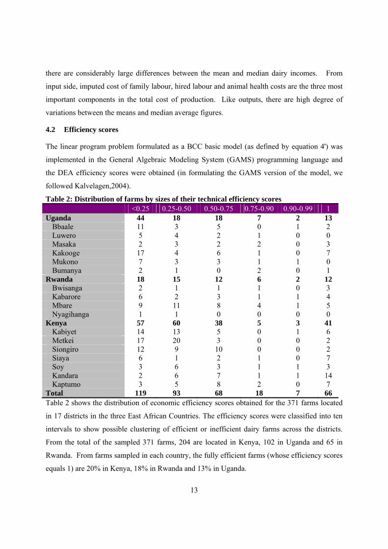
Table 2: Distribution of farms by sizes of their technical efficiency scores <0.25 0.25-0.50 0.50-0.75 0.75-0.90 0.90-0.99 1 Uganda 44 18 18 7 2 13 Bbaale 11 3 5 0 1 2 Luwero 5 4 2 1 0 0 Masaka 2 3 2 2 0 3 Kakooge 17 4 6 1 0 7 Mukono 7 3 3 1 1 0 Bumanya 2 1 0 2 0 1

Rwanda 18 15 12 6 2 12 Bwisanga 2 1 1 1 0 3 Kabarore 6 2 3 1 1 4 Mbare 9 11 8 4 1 5 Nyagihanga 1 1 0 0 0 0

Kenya 57 60 38 5 3 41 Kabiyet 14 13 5 0 1 6 Metkei 17 20 3 0 0 2 Siongiro 12 9 10 0 0 2 Siaya 6 1 2 1 0 7 Soy 3 6 3 1 1 3 Kandara 2 6 7 1 1 14 Kaptumo 3 5 8 2 0 7

Total 119 93 68 18 7 66 Table 2 shows the distribution of economic efficiency scores obtained for the 371 farms located

in 17 districts in the three East African Countries. The efficiency scores were classified into ten

intervals to show possible clustering of efficient or inefficient dairy farms across the districts.

From the total of the sampled 371 farms, 204 are located in Kenya, 102 in Uganda and 65 in

Rwanda. From farms sampled in each country, the fully efficient farms (whose efficiency scores

equals 1) are 20% in Kenya, 18% in Rwanda and 13% in Uganda.

14

As noted earlier, a farm with an efficiency score of 0.25 would need to increase output by 75% to

reach the efficiency frontier without any increase in the level of input used in the process of

production. Table 2 shows that 119 of the 371 farms have efficiency scores less than or equal to

0.25, which means that about 32% of the farms would need to increase milk output by at least

75% to reach the production frontier already reached by other dairy farms in the region. In

Uganda, this proportion is even higher, with 43% of the farms needing to increase dairy

production by making best use of inputs already at their disposal. The corresponding proportion

of farms in this group in Kenya and Rwanda are 28% in each case. Overall, close to a third of all

farms in the sample will need to increase output by at least 50% to reach the production frontier

holding the level of input at the current level. This shows that there is considerable degree of

improvement. It should be noted that the efficiency scores reported here are derived from the

BCC basic model which means that it does not include scale effects.

Table 3: Descriptive statistics of the technical efficiency scores in the farms Scores Mean SD Min Median Max

<0.25 0.149 0.064 0.002 0.151 0.250 0.25-0.50 0.362 0.069 0.252 0.355 0.498 0.50-0.75 0.622 0.074 0.502 0.619 0.750 0.75-0.90 0.826 0.053 0.755 0.832 0.895 0.90-0.99 0.941 0.034 0.904 0.935 0.999

1.00 1.000 0.000 1.000 1.000 1.000 Total 0.488 0.323 0.002 0.410 1.000

Table 3 below provides additional information on summary statistics of the efficiency scores,

primarily to show the distribution of the scores within each interval reported in Table 1. For

instance, the mean averages for those farms with efficiency scores less than 0.25 was 0.15.

5 ECONOMERIC ANALYSIS

5.1 Model specification

As noted earlier, the second stage involves a regression analysis to relate DEA efficiency scores

to exogenous factors. The econometric analysis is required to seek explanation as to why the

DEA efficiency scores vary so much between farms and locations. Ramalho et al., (2010)

provide a useful summary of how misspecification of the second-stage regression model may

generate misleading results. The bounded nature of DEA scores limits the application of

15

standard regression models to DEA scores. It is important to note that the values of the efficiency

scores lie between 0 and 1. Critically, however, the efficiency scores do not take a value of zero

which means Ө is strictly greater than 0 (Ө > 0). However, since fully efficient farms do exist, Ө

can take a value of 1, which means that Ө ≤ 1. Thus, the realistic range of the values of DEA

efficiency scores would be 0< Ө ≤ 1. The unique combinations o f weak and strong inequalities

bounding the range of values for DEA scores would have an important implication for the choice

of econometric models.

In the DEA literature, a range of standard regressions are employed to explain DEA scores.

These include ordinary, generalised, or truncated least squared regressions (Helfand and Levine

2004; Johansson 2005; Kolawole, 2009; O’Donnell and Coelli , 2003), ordered logistic

regression (Usmay et al., 2009) and Tobit analysis (Alexander, 2003). However, as Ramalho et

al. (2010, p. 2) observed, the standard linear models may not be appropriate because the

predicted values may lie outside the unit interval and the implied constant marginal effects of the

covariates on are not compatible with both the bounded nature of DEA scores and the existence

of a mass point at unity in their distribution.

In this study we follow a fractional regression approach proposed by Papke and Wooldridge

(1996) which pioneered direct models for the conditional mean of the fractional response that

keep the predicted values in the unit interval through a more refined and flexible analyses using

the generalized linear model (GLM). Papke and Wooldridge’s (2007) provides further

developments and applications of this method, a quasi-maximum likelihood estimation (QMLE)

to obtain robust estimators of the conditional mean parameters with satisfactory efficiency

properties. Moreover, a Stata code known as fractional logit,” or “flogit” was developed and has

simplified the implementation of the quasi-MLE with a logistic mean function.

5.2 Results

5.2.1 Descriptive analysis

Table 4below displays descriptive statistics for variables used in the econometric estimation.

The explanatory variables can be classified into broad categories. The first category is related to

household characteristics: age of household head, farming experience in years, education level,

and family size. The mean and median age household head was 50 and 49 years respectively.

16

The average years of farming experience is 25 and average family size was about 5. The number

of years of schooling is about 7.

Table 4: Descriptive statistics for the sample of dairy households Mean SD Min Max Median

Age of household head (years) (AGEHH) 50.2 15.1 18 100 49 Farming exp. of hh head (yrs) (FAEXHH) 24.7 15.8 1 75 21.5 Family size (adult equivalent) (FAMILY) 4.9 2.1 0.82 14.25 4.6 Edu. level of hh head (yrs) (EDUCATIONHH) 6.8 4.6 0 25 7 Farm size (acres) (FARM) 43.9 134.3 0.25 960 6 Number of cattle (TLU)3 15.9 26.7 0.7 277.2 7.85 Ratio of improved breeds (RATIO_IMBRDS) 0.5 0.5 0 1 0.6 Off-farm income (OFF-FARM) Yes: 192 (1) No: 179 (0) Member in a dairy coop. (DAIRYCOOP) Yes: 53 (1) No: 318 (0) Practice zero grazing (ZERO_GRAZING) Yes: 37 (1) No:334 (0) Conserve feed (FEED_CONSERVE) Yes: 69 (1) No: 302 (0) Grow fodder legumes (LEGUMES) Yes: 20 (1) No: 351 (0) Milk buyer dummies Individual customers: 97; Private traders: 117;

Dairy coop.: 45; Chilling plant: 29 Country dummies Uganda: 102; Rwanda: 65; Kenya: 204 Recommendation domains4 HH: 155; HL: 81; LH: 33 LL:102 The second group of explanatory variables are farm assets: farm size, number of cattle in tropical

livestock units (TLUs), the proportion of improved breeds in the total number of livestock kept

on the farm. The average farm size was 44 acres but there is a large variation among the farming

households. The mean average TLUs owned by the households was about 16 but about 50% of

the households actually keep less than 8. On average, half of the cattle kept on farm are

improved breed. The econometric estimation also included a range of dummy variables which

are expected to positively or negatively affect performances of the dairy farms. The latter group

of variables are intended to capture a range of qualitative factors such as livestock management,

technology adoption, marketing and agro-ecological conditions.

3 TLU stands for Tropical Livestock Unit calculated by multiplying TLU factor and TLU breed factor. For example TLU factor for a cow is 1, while TLU breed factor for a Holstein-Friesian (pure) breed is 1.6. If a farmer has got 1 Holstein –Friesian pure cow, total TLU of that cow is 1*1.6=1.6 4 EADD sites were selected based on 2 domains: Market access and Length of Growth Period (LGP), hence HH represents a site with High market access and High LGP, LL, site with Low market access and Low LGP, HL, High market access and Low LGP, LH, Low market access and High LGP.

17

5.2.2 Estimates

Starting with household characteristics, education level and farming experience of the head of

the household has a positive effect on farm efficiency but household age and family size have

negative effects. However, none of the variables in this group seem to have a statistically

significant effect on dairy farm efficiency. Off-farm income has negative but insignificant

effect.

From the three variables denoting farm assets in the model, the size of livestock (in TLUs)

owned by the household does not only have a relatively large positive effect, but also its effect is

highly significant at 1%. This could be associated with high levels of output (milk, cattle sales)

derived from large cattle herds. It implies that 1% increase in number of cattle (in terms of TLU),

increases the farm efficiency by 0.0033 units (0.3286/100). The results also agree with a study

conducted in Wales England, where farms with a larger number of cows were found to be more

efficient (Gerber and Franks, 2001). Similarly, the proportion of improved breeds in total

livestock kept on farm also has a positive and statistically significant effect at 10% level. This

could also explain the positive coefficient of the ratio of improved breeds in the herd, where a

unit increase in one unit of improved breed increases the efficiency levels by 45%. However,

although the size of farm owned by the household has a positive influence, this is not statistically

significant.

18

Table 5 provides a summary of econometric results of the model. In order to ensure that the data

is uniformly distributed, most level form variables were transformed to log form. These include

age of household head, farming experience of the household head, family size, level of education

of the household head, farm size; and number of cattle owned. Using log transforms enables

modeling a wide range of meaningful, useful, non-linear relationships between dependent and

independent variables (Shmueli, 2009). Using log-transform moves from unit-based

interpretations to percentage-based interpretations (Vittinghoff, Glidden, Shiboski & McCulloch,

2004).

Starting with household characteristics, education level and farming experience of the head of

the household has a positive effect on farm efficiency but household age and family size have

negative effects. However, none of the variables in this group seem to have a statistically

significant effect on dairy farm efficiency. Off-farm income has negative but insignificant

effect.

From the three variables denoting farm assets in the model, the size of livestock (in TLUs)

owned by the household does not only have a relatively large positive effect, but also its effect is

highly significant at 1%. This could be associated with high levels of output (milk, cattle sales)

derived from large cattle herds. It implies that 1% increase in number of cattle (in terms of TLU),

increases the farm efficiency by 0.0033 units (0.3286/100). The results also agree with a study

conducted in Wales England, where farms with a larger number of cows were found to be more

efficient (Gerber and Franks, 2001). Similarly, the proportion of improved breeds in total

livestock kept on farm also has a positive and statistically significant effect at 10% level. This

could also explain the positive coefficient of the ratio of improved breeds in the herd, where a

unit increase in one unit of improved breed increases the efficiency levels by 45%. However,

although the size of farm owned by the household has a positive influence, this is not statistically

significant.

19

Table 5: Results of the General linear model (GLM) with robust standard errors of factors influencing farm efficiency levels Variable description Coefficient Robust

Standard Error

z P>z 95% Conf. interval

Log (AGEHH) -0.1072 0.4310 -0.25 0.804 -0.9519288 - 0.737583Log (FAEXHH) 0.0003 0.1733 0 0.999 -0.3394249 - 0.339926Log (FAMILY) -0.2671 0.2092 -1.28 0.202 -0.677216 - 0.142919Log (EDUCATIONHH) 0.1948 0.1420 1.37 0.17 -0.0835866 - 0.473103 OFF-FARM -0.0343 0.1779 -0.19 0.847 -0.3828521 - 0.314321 Log (FARM) 0.0372 0.0710 0.52 0.601 -0.1020264 - 0.176422Log (TLU) 0.3286 0.1136 2.89 0.004*** 0.1059005 - 0.551353RATIO_IMBRDS 0.4463 0.2381 1.87 0.061* -0.0203208 - 0.912886 LEGUMES 0.9892 0.3340 2.96 0.003*** 0.3345673 - 1.643893ZERO_GRAZING 1.0669 0.3347 3.19 0.001*** 0.4108981 - 1.722895FEED_CONSERVE -0.1988 0.2191 -0.91 0.364 -0.6282585 - 0.23066 DAIRYCOOP 0.3163 0.2363 1.34 0.181 -0.1468431 - 0.779359Individual customer milk buyer dummy

0.6379 0.2331 2.74 0.006*** 0.1811201 - 1.094715

Private milk trader dummy

-0.0251 0.2274 -0.11 0.912 -0.4708374 - 0.420659

Chilling plant dummy -0.0547 0.2585 -0.21 0.833 -0.5613117 - 0.451973 Uganda_dummy -0.6112 0.3193 -1.91 0.056* -1.237075 - 0.014682Kenya_dummy -0.2045 0.3556 -0.58 0.565 -0.9015913 - 0.492519HH dummy 0.2591 0.3251 0.8 0.425 -0.3780425 - 0.896324HL dummy 0.5766 0.3857 1.49 0.135* -0.1793695 - 1.332573LL dummy -0.0505 0.3439 -0.15 0.883 -0.7244115 - 0.623501Constant -0.9004 1.3993 -0.64 0.52 -3.642934 - 1.842036Deviance = 90.22799027 No. of obs = 227 Pearson = 75.05593911 Residual df = 206 Variance function: V(u) = u*(1-u/1) [Binomial] Scale parameter = 1 Link function : g(u) = ln(u/(1-u)) [Logit] (1/df) Deviance = 0.438 Log pseudolikelihood = -113.5536042 AIC = 1.185494 (1/df) Pearson = 0.3643492 BIC = -1027.312 Note: *=Statistically significant at 10%; **=Statistically significant at 5%; ***=Statistically significant at 1%

20

The econometric results suggest growing fodder and and/or practice zero-grazing has a highly

significant effect (both at 1%) on hat dairy farms efficiency. On the other hand, feed

conservation seems to have a rather unexpected negative effect although this is not statistically

significant. In terms of marketing outlets or buyer types, selling directly to consumers (e.g.

neighbors, organizations, etc) has a strongly positive and statistically significant influence on

dairy farm efficiency. The interpretation of the coefficient suggests that selling of milk to

individual customers increases the efficiency levels by about 63%. . Contrary to our expectation,

although not significant, sale of milk to a chilling plant was found to be negatively associated

with efficiency scores. Membership of dairy cooperatives does have a positive effect but not

significant statistically.

The coefficient of Uganda dummy in the model is significant and negative. This implies that,

efficiency levels of farms located in Uganda are 60% less compared to the other countries. In

terms of recommendation domain, it was expected that sites with high market access and high

LGP would be more efficient. The HH (high market access/ high LGP) domain however was not

significant but positive. The coefficient of the HL (high market access/ low LGP) was positive

and significant. This suggests that, the location of a site in an area with high market access and

low LGP is associated with 57% increase in efficiency level.

6 CONCLUSIONS

The study was set out to measure and explain economic efficiency of dairy farms sampled from

seventeen districts in three East African Countries. A DEA methodology was used to measure

out-put oriented efficiency scores, which were obtained allowing variable returns to scale. The

latter condition is suitable to conditions of dairy farming in East Africa where various constraints

inhibit dairy farms from realizing their potentials by expanding their scales of operation.

One of the main findings of this study is to establish the extent to which dairy farms in the region

are operating at a considerably high level of inefficiency. On the one hand, from farms sampled

in each country, the fully efficient farms (whose efficiency scores equals 1) are 20% in Kenya,

18% in Rwanda and 13% in Uganda. On the other hand, about 32% of the 371 farms studied

would need to increase milk output by at least 75% to reach the production frontier already

21

reached by other dairy farms in the region. In Uganda, this proportion is even higher, with 43%

of the farms needing to increase dairy production by making best use of inputs already at their

disposal. The corresponding proportion of farms in this group in Kenya and Rwanda are 28% in

each case. Overall, close to a third of all farms in the sample will need to increase output by at

least 50% to reach the production frontier holding the level of input at the current level.

We have gone further and examined determinant factors for dairy farm efficiency. Technology

adoption factors such as existence of improved breeds in the herd and feed and fodder

innovations (whether or not the farmer is growing legumes, etc) have positive and statistically

significant effect on the levels of economic efficiency. Similarly, farms practicing zero grazing

are characterized by high level of economic efficiency.

Some of the most surprising findings in this study are related to marketing factors. Contrary to

what was expected, membership of dairy cooperatives or selling to chilling plants has negative

but not statistically insignificant effect on dairy performance. Interestingly, selling directly to

consumers or institutions seems to be more associated with improvements in economic

performances of dairy farms. Further investigations into the latter intriguing results are left for

subsequent research.

22

References Charnes A, Cooper WW, Rhodes E (1978). Measuring the efficiency of decision-making units. European Journal of Operational Research 1978, 2: 429-444. Aggrey N., Eliab L. and Joseph S. , (2010). Export Participation and Technical Efficiency in East African Manufacturing Firms. Research Journal of Economic Theory 2(2): 62-68. Aggrey N., Eliab L. and Joseph S. , (2010). Firm Size and Technical Efficiency in East African Manufacturing Firms. Current Research Journal of Economic Theory 2(2): 69-75. Alexander C. A. Busch G. and Stringer K., (2003). Implementing and interpreting a data envelopment analysis model to assess the efficiency of health systems in developing countries. IMA Journal of Management Mathematics 14: 49–63. Amos T. T., (2007). An Analysis of Productivity and Technical Efficiency of Smallholder Cocoa Farmers in Nigeria. Journal of Social Sciences,15(2): 127-133 (2007). Baltenweck, Isabelle, Gelan, Ayele and Muriithi, Beatrice (2009). East African Dairy Development Project Baseline Surveys Report No.1: Survey Methodology and Overview of Key Results for the Household Surveys Banker, R.D., Charnes, A. and Cooper, W. W.(1984). Some Methods for Estimating Technical and Scale Inefficiencies in Data Envelopment Analysis. Management Science 30: 1078-1092 Chirwa E. W., (2007). Sources of Technical Efficiency among Smallholder Maize Farmers in Southern Malawi. African Economic Research Consortium (AERC), Research Paper 172. Coelli T., (2008). A Guide to DEAP Version 2.1: A data Envelopment Analysis (Computer) program. Center for Efficiency and Productivity Analysis (CEPA), Working Paper 96/08. Available at http://www.une.edu.au/econometrics/cepa.htm. Coelli T., Hajargasht G. and Lovell C.A. K., (2008). Econometric Estimation of an Input Distance Function in a System of Equations. Center for Efficiency and Productivity Analysis (CEPA), Working Paper, No. WP01/2008. Coelli, T. and Perleman, S. (1999). A comparison of parametric and non-parametric distance functions: With application to European railways. European Journal of Operational Research 117: 326-339 Cooper W. W., Seiford L. M., and Zhu J. (2010). Data Envelopment Analysis. History, Models and Interpretations. Handbook on Data Envelopment Analysis, 71: 1-39. Springer. DOI: 10.1007/b105307 Dlamini S., Rugambisa J. I., Masuku M. B., and Belete A., (2010). Technical efficiency of the small scale sugarcane farmers in Swaziland: A case study of Vuvulane and Big bend farmers.

23

African Journal of Agricultural Research ,5(9): 935-940. Fethi M. D., Jackson P. M., Weyman-Jones T. G., ( 2001). Measuring the Efficiency of European Airlines: An Application of DEA and Tobit Analysis Management Centre. Efficiency and Productivity Research Unit (EPRU) Discussion Papers, University of Leicester. Available at http://hdl.handle.net/2381/372. Førsund F. R., (2001). Categorical Variables in DEA. “Cheaper and better?” project, Department of Economics, University of Oslo, Norway and ICER, Turin, Italy, January – March 2001. Fullerton A. S., (2009). A Conceptual Framework for Ordered Logistic Regression Models. Sociological Methods & Research, 38(2): 306–347. Gerber, J., and J. Franks, (2001). Technical efficiency and benchmarking in dairy enterprises. J. Farm Manage., 10 (12): 715-728. Johansson, Helena (2005). Technical, allocative, and economic efficiency in swedish dairy farms: the data envelopment analysis versus the stochastic frontier approach. Poster background paper prepared for presentation at the 11th International Congress of the European Association of Agricultural Economists (EAAE), Copenhagen, Denmark, August 24-27, 2005 Kalvelagen, Erwin (2004). Efficiently solving DEA models with GAMS, http://www.amsterdamoptimization.com/pdf/dea.pdf (last accessed: 30/5/2010) Kolawole O., (2009). A Meta-Analysis of technical efficiency in Nigerian agriculture. Contributed Paper prepared for presentation at the International Association of Agricultural Economists Conference, Beijing, China, August 16-22, 2009. Available at http://ageconsearch.umn.edu/bitstream/50327/2/238.pdf. Murova O. I., Trueblood A.M.. and Coble H. K., (2004). Measurement and Explanation of Technical Effificency Performance in Ukrainian Agriculture, 1991-1996. Journal of Agricultural and Applied Economics, 36, 1: 185-198.

Nkamleu G. B., (2003). Productivity Growth, Technical Progress and Efficiency Change in African Agriculture. African Development Bank. Tunisia, MPRA Paper No. 11380. Available from http://mpra.ub.uni-muenchen.de/11380/.

O’Donnell C. and Coelli T., (2003). A Bayesian Approach To Imposing Curvature on Distance Functions. Centre for Efficiency and Productivity Analysis (CEPA), Working Paper, No. 03/2003. Papke L.E. and Wooldridge J. M., (2007). Panel data methods for fractional Response variables with an application to test pass rates. Department of Economics, Michigan State University. Ramalho E. A., Ramalho J. J.S. and Henriques P. D., (2010). Fractional regression models for second stage DEA efficiency analyses. CEFAGE-UE Working Paper 2010/01.

24

Resti, Andrea (1997). Evaluating the cost-efficiency of the Italian Banking System: What can be learned from the joint application of parametric and non-parametric techniques. Journal of Banking & Finance. 21: 221-250. Sampaio de S. M., Cribari-Neto F. and Borko D., (2005). Explaining DEA Technical Efficiency Scores in an Outlier Corrected Environment: The Case of Public Services in Brazilian Municipalities. Brazilian Review of Econometrics 25(2): 287–313 Shmueli G., (2009). Interpreting log-transformed variables in linear regression. Posted in the Bzst, Musings on Business and statistics (oops, data analysis). Retrieved May 27, 2010, at http://blog.bzst.com/2009/09/interpreting-log-transformed-variables.html Staal, S., Owango, M., Muriuki, H., Kenyanjui, M., Lukuyu, B., Njoroge, L., Njubi, D., Baltenweck, I., Musembi, F., Bwana, O., Muriuki K., Gichungu, G., Omore, A. and Thorpe, W. 2001. Dairy systems characterisation of the greater Nairobi milk shed. Smallholder Dairy (R&D) Project report. Availble at: http://www.smallholderdairy.org/collaborative%20res%20reports.htm Stokes J. R., Tozer P. R., and Hyde J., (2007). Identifying Efficient Dairy Producers Using Data Envelopment Analysis . Journal of Dairy Science 90:2555–2562. DOI:10.3168/jds.2006-596 Theodoridis, A. M. and Psychoudakis, A., (2008). Efficiency Measurement in Greek Dairy Farms: Stochastic Frontier vs. Data Envelopment Analysis. International journal of economic sciences and applied research (IJESAR) 1(2): 53-67. Trana N. A., Shivelyb G., and Preckelb P., (2008). A new method for detecting outliers in Data Envelopment Analysis. Applied Economics Letters, 2008, 1–4, iFirst. DOI: 10.1080/13504850701765119. Uzmay A., Koyubenbe and Armagan G., (2009). Measurement of Efficiency Using Data Envelopment Analysis (DEA) and Social Factors Affecting the Technical Efficiency in Dairy Cattle Farms within the Province of Izmir, Turkey. Journal of Animal and Veterinary Advances 8 (6): 1110-1115, 2009. Vanden Eng, Jodi L, et al. (2007). Use of Handheld Computers with Global Positioning Systems for Probability Sampling and Data Entry in Household Surveys. American Journal of Tropical Medicine and Hygiene 77(2): 393-399

Vittinghoff, E., Glidden, D., Shiboski, S., McCulloch, C.E. (2005). Regression Methods in Biostatistics: Linear, Logistic, Survival, and Repeated Measures Models. 16: 344-

Appendix 1 - Project areas for East Africa Dairy Development Project

25

26

Appendix 2 – schematic representation of the geographic sampling frame

Sampled grid cell

‘Site’ Hub

Masked out area

27

Appendix 3 - Rwanda - Bwisanga/Gasi (Rwamagana district)