Measuring and Modeling Determinants of Fiscal Stress in

US Municipalities

Evgenia Gorina and Craig Maher

November 2016

MERCATUS WORKING PAPER

Evgenia Gorina and Craig Maher. “Measuring and Modeling Determinants of Fiscal Stress in US Municipalities.” Mercatus Working Paper, Mercatus Center at George Mason University, Arlington, VA, November 2016. Abstract The Great Recession produced a wave of fiscal crises in cities and counties throughout the United States. In addition to high-profile bankruptcy filings in Detroit, Michigan, and Harrisburg, Pennsylvania, many local governments declared fiscal emergencies, cut spending, and laid off or furloughed workers. Yet some municipalities weathered the recession without such actions. In this paper, we explore the factors that help predict the likelihood of local fiscal distress. We construct a measure of fiscal distress using annual financial reports, budgets, and media coverage, and we then use this measure as a dependent variable to model fiscal distress as a function of past financial performance, real estate prices, and socioeconomic environment. This work adds to the existing literature in several ways. First, the proposed measure of fiscal distress is based on government actions and therefore has greater external validity than measures based on financial indicators. Second, we add to the literature that goes beyond the measurement of fiscal distress and focuses on its prediction. Finally, we offer policy-relevant conclusions by showing the relative importance of fiscal reserves, revenue composition, and real estate pricing in predicting local fiscal distress. JEL codes: H71 Keywords: government finance, municipalities, fiscal crisis, fiscal distress, fiscal emergency, budget, debt burden, revenue structure, fiscal reserves Author Affiliation and Contact Information Evgenia Gorina Craig Maher Assistant Professor, Program in Public and Director, Nebraska State & Local Nonprofit Management Finance Lab School of Economic, Political and Policy Sciences School of Public Administration University of Texas at Dallas University of Nebraska at Omaha egorina@utdallas.edu csmaher@unomaha.edu All studies in the Mercatus Working Paper series have followed a rigorous process of academic evaluation, including (except where otherwise noted) at least one double-blind peer review. Working Papers present an author’s provisional findings, which, upon further consideration and revision, are likely to be republished in an academic journal. The opinions expressed in Mercatus Working Papers are the authors’ and do not represent official positions of the Mercatus Center or George Mason University.

3

Measuring and Modeling Determinants of Fiscal Stress in US Municipalities

Evgenia Gorina and Craig Maher

Introduction

In the past decade, a wave of fiscal crises has hit cities and counties throughout the United

States. In California, Vallejo, Stockton, and San Bernardino have filed for bankruptcy. Michigan

has declared financial emergencies in Detroit, Flint, and several smaller cities (Convery and

Imdieke 2015; Scorsone 2014). Like Michigan, Pennsylvania has stepped in to manage financial

crises in a number of cities and boroughs, including Scranton, Altoona, and Harrisburg. In

addition to these exceptional cases of fiscal distress, the 2007–09 recession negatively affected

many other cities and counties (Hoene and Pagano 2009), forcing some of them to declare fiscal

emergencies, default on debt, or lay off and furlough workers. In this paper, we propose an

evidence-based measure of fiscal distress and examine which of the theoretically relevant factors

can be used to effectively predict fiscal distress before it hits crisis stage.

Background

The attention to local government fiscal condition and fiscal distress is not new. Scholars and

practitioners have been trying to resolve measurement and prediction questions related to

government fiscal condition for decades. Ever since the near-meltdown of New York’s finances

in the 1970s, public finance researchers, governments, and professional organizations have

sought to provide analytical tools for measuring fiscal condition to prevent a repeat. A pioneer in

this area was the Advisory Commission on Intergovernmental Relations (ACIR), which

produced a series of studies focusing on state and local government fiscal capacity throughout

the 1970s and 1980s (ACIR 1971, 1979, 1981, 1988, 1989). In the 1980s, work by Levine,

4

Rubin, and Wolohojian (1981), Rubin (1982), Berne and Schramm (1986), Groves and Valente

(1986), Pammer (1990), and others laid out comprehensive theoretical frameworks for

examining local fiscal condition and developed a broad theoretical understanding of various

dimensions of government fiscal health. By the 1990s, academic interest in fiscal health slightly

waned, as evidenced by the lower number of publications during the decade. Some of these

publications, however, became highly influential, including the second edition of “Evaluating

Financial Condition: A Handbook for Local Government” by Groves and Valente (1994), also

known as the financial trends monitoring system (FTMS). Interest in local government fiscal

health recovered after 2000. By 2003, the International City/County Managers Association’s

(ICMA) FTMS was in its fourth edition (Nollenberger, Groves, and Valente 2003).

Since the 1990s, with the exception of ICMA’s FTMS, most innovative empirical

research on fiscal condition has appeared in journals or edited volumes (e.g., Brown 1993;

Chaney, Mead, and Schermann 2002; Hendrick 2004; Chaney 2005; Kloha, Weissert, and Kleine

2005; Frank 2006; Mead 2006; Kravchuk and Stone 2010; Rivenbark, Roenigk, and Allison

2010; Clark 2015). In 2013, the diversity of approaches to the analysis and management of fiscal

condition was reflected in the Handbook of Local Government Fiscal Health, edited by Levine,

Justice, and Scorsone (2013), which brought together a cohort of leading fiscal health

researchers. The edited volume demonstrates that while there is some agreement on fiscal health

as a theoretical concept, there is still little consensus on how to measure, predict, and manage a

decline in fiscal health (Justice and Scorsone 2013). Importantly, empirically based studies that

would test the external validity of the proposed measures of fiscal health are particularly lacking,

although some of this work has been started by Clark (2015) and Stone et al. (2015).

5

Often guided by academic research, a number of states have adopted fiscal condition

monitoring systems for their local governments over the past two decades, including New York

(Office of the State Comptroller 2015), North Carolina (Coe 2007), Michigan (Kloha, Weissert,

and Kleine 2005; Crosby and Robbins 2013), Ohio (Clark 2015), and Pennsylvania

(Pennsylvania Department of Community and Economic Development 2011). The fiscal

condition monitoring system proposed by Kloha et al. (2005), a blueprint for the Michigan state

monitoring system, is an example of a relatively efficient fiscal health assessment for a large

number of communities. It is based on the analysis of population changes, trends in real taxable

property values, general fund expenditures, general fund operating position, and general long-

term debt. Though the system does provide a useful assessment of the relative fiscal health of

Michigan communities, the efficiency of the system comes at the expense of its accuracy. Since

it uses absolute benchmarks to create binary scores (0 or 1) for various indicators of a

government’s performance which it then sums into a cumulative score, the system is prone to

measurement error (Crosby and Robbins 2013). Besides, like its predecessor, Brown’s 10-point

test of municipal financial condition (Brown 1993), the Kloha et al. system focuses on

municipalities’ general fund, excludes enterprise funds, and ignores such long-term liabilities as

pension obligations and other post-employment benefits (Crosby and Robbins 2013; Justice and

Scorsone 2013; Plerhoples and Scorsone 2011).

We build on the existing body of literature to select indicators of fiscal distress that

would effectively capture key measurable dimensions of local fiscal health. In contrast to the

dominant empirical literature, we determine the fiscal distress status of a government based on

its behavior, which often manifests as politically difficult fiscal decisions to address fiscal

distress. In this respect, we offer an alternative approach to conducting empirical research on the

6

prediction of fiscal distress. The “behavioral” measure of fiscal distress becomes our dependent

variable, and the fiscal and socioeconomic indicators work as predictors.

The structure of this paper is as follows. The next section offers an overview of the

literature that guided us toward the choice of fiscal health predictors. We then present the

Conceptual Framework used in this study. The Data and Method section describes the dependent

variable, the independent variables, and the empirical models. In Results, we present and interpret

the findings. The Discussion and Conclusion section highlights the paper’s implications for the

theory of fiscal health research and offers two suggestions for the practice of fiscal management.

Literature Overview

What Is Fiscal Condition?

Fiscal condition is typically understood as a position on a spectrum of financial “wellness”

commonly referred to as fiscal health. Many local government researchers agree that “[a] host of

factors affect local government finances, and no single metric is able to fully account for the

various components of financial condition” (Jacob and Hendrick 2013, 11). It is often suggested

that fiscal condition is shaped by local decisions and the external environment (Honadle, Costa,

and Cigler 2004; Hendrick 2011; Nollenberger, Groves, and Valente 2003). As a result, an

analysis of local fiscal condition or fiscal health often involves an analysis of the government’s

environment, its fiscal structure, and the balance of fiscal structure with the environment

(Hendrick 2004, 2011). From this perspective, the key to fiscal health is to adapt fiscal decisions

to the environment (Hendrick 2011). The environment may be viewed broadly and may include a

variety of factors, from immediate economic resources to political culture (Clark and Ferguson

7

1983). Conceptually, whenever fiscal decisions and available resources are misaligned, a

government experiences fiscal stress (Chapman 2008).

Fiscal Condition Metrics

Perhaps the most comprehensive practitioner-oriented framework for fiscal condition monitoring

was developed by the ICMA (Groves and Valente 1983, 1994; Nollenberger, Groves, and

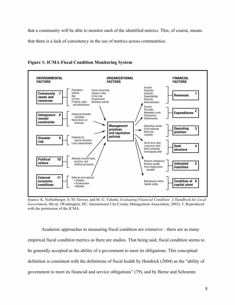
Valente 2003). The FTMS framework distinguishes among three types of factors that influence

fiscal health: environmental, organizational, and financial. Environmental factors consist of those

over which the community has little or no control: the external economy, intergovernmental

constraints, community socioeconomic characteristics, disaster risk, and political culture.

Organizational factors involve government practices and policies and largely remain a black box

in the framework. Financial factors are the outcomes of organizational decisions with regard to

available environmental resources and opportunities. Financial factors manifest as measures of

revenues, expenditures, operating position, long-term liabilities, and asset maintenance. The

environmental factors are predicted to affect government practices and policies, which in turn are

predicted to affect the entity’s financial condition.

The ICMA framework offers 48 potentially useful indicators of fiscal condition that

characterize four dimensions of local fiscal condition: cash solvency, budgetary solvency, long-

term solvency, and service solvency. Since local financial arrangements vary, the ICMA

framework suggests that governments should choose the metrics they deem important and track

them over time. Then, based on the direction of the trends, communities can determine whether

their financial condition is improving, declining, or staying the same. There is no benchmarking

relative to other entities and—given the complexity and breadth of the measures—no expectation

8

that a community will be able to monitor each of the identified metrics. This, of course, means

that there is a lack of consistency in the use of metrics across communities.

Figure 1: ICMA Fiscal Condition Monitoring System

Source: K. Nollenberger, S. M. Groves, and M. G. Valente, Evaluating Financial Condition: A Handbook for Local Government, 4th ed. (Washington, DC: International City/County Management Association, 2003), 5. Reproduced with the permission of the ICMA.

Academic approaches to measuring fiscal condition are extensive—there are as many

empirical fiscal condition metrics as there are studies. That being said, fiscal condition seems to

be generally accepted as the ability of a government to meet its obligations. This conceptual

definition is consistent with the definitions of fiscal health by Hendrick (2004) as the “ability of

government to meet its financial and service obligations” (79), and by Berne and Schramm

9

(1986) as “the probability that a government will meet its financial obligations” (71). This study

uses the notions of fiscal health and fiscal condition synonymously.

The empirical frameworks of fiscal condition tend to incorporate measures of revenues and

expenditures, operating position, and fiscal flexibility (Berne and Schramm 1986; Hendrick 2004;

Kloha, Weissert, and Kleine 2005). Measures of revenue and expenditure capacity have also

received attention. For example, some scholars have combined revenue capacity and spending

needs to create a measure of “need-capacity gap” (Ladd and Yinger 1989) or “standardized fiscal

health” (Chernick and Reschovsky 2006; Skidmore and Scorsone 2010). Hendrick (2004)

measured revenue capacity as own-source revenues relative to city wealth (tax base, personal

income, and sales receipts). Maher and Nollenberger (2009) created a proxy for revenue capacity

using general-fund revenues per capita, intergovernmental revenues as a percentage of total

revenues, and own-source tax revenues as a percentage of general-fund revenues.

Financial Reporting Effects

As the measurement of fiscal condition has evolved, so has financial reporting. The most

important change in financial reporting was GASB 34, which was adopted in 1999 and required

governments to produce accrual-based government-wide financial statements. Chaney (2005)

and Chaney, Mead, and Schermann (2002) offered some of the first fiscal condition metrics

based on government-wide statements. This work was followed by Wang, Dennis, and Tu

(2007), who assessed the validity of government-wide ratios; Rivenbark, Roenigk, and Allison

(2010), who offered a practical approach for local officials to collect data and explain financial

condition using government-wide ratios; and Arnett (2012), whose dissertation focused on state-

level financial condition analysis using government-wide statements. The purpose of the

10

measures using government-wide statements remained the same—to capture changes in four

commonly identified dimensions of fiscal health: cash solvency, budgetary solvency, long-run

solvency, and service-level solvency. The benefits of government-wide statements over fund

statements include an opportunity to capture long-term liabilities such as pension obligations and

an opportunity to uniformly report on government assets and liabilities beyond the general fund

(Mead 2013). More recent fiscal condition ratios include a combination of fund and government-

wide statements (Mead 2013; Maher 2013). Despite efforts to demonstrate the validity of the

ratios based on government-wide statements (particularly by Wang, Dennis, and Tu 2007),

government-wide measures have recently been challenged by Clark (2015).

Evaluating Fiscal Condition

In addition to a variety of possible indicators of fiscal condition, several approaches have been

developed to combine the indicators into a single measure of fiscal condition. Brown (1993)

offered a cumulative score of fiscal condition based on a community’s quartile ranking on each

of the 10 indicators. Kloha, Weissert, and Kleine (2005) came up with relative benchmarks for

each indicator, assigned the score of 1 to governments that met a benchmark and 0 otherwise,

and then summed the scores for each indicator into a single aggregate score. Mead (2006)

revised Brown’s test to include indicators of pension funding. Yet Hendrick (2004) asserted that

fiscal health is too complicated to combine into one single score and that “measures of [different]

dimensions should be constructed separately and assessed in relation to one another to produce a

complete and more accurate picture of fiscal conditions” (85). In this respect, rating agency

credit ratings offer a compromise between a single score and a vast variety of indictors. A credit

rating consolidates all relevant information about a government into a single metric, while

11

allowing for a categorical differentiation of fiscal conditions through rating grades. Importantly,

when credit rating agency analysts construct a rating, they analyze both quantitative and

qualitative information. However, since the investor community takes changes in government

credit ratings seriously, changes in rating tend to be made conservatively (when a critical mass of

evidence is collected) and may lag behind an actual change in fiscal condition.

Where Are We Now?

Despite the extent of the academic and professional literature and the increasingly widespread

use of metrics of fiscal condition in modern management practices (for a review, see Stone et al.

2015), fiscal condition measurement issues are yet to be resolved, and empirical methodologies

for predicting fiscal distress are yet to be perfected. Importantly, there is a growing

understanding that indicators of fiscal condition need to be validated against some objective

reality of whether a government is experiencing fiscal prosperity or distress (Clark 2015; Stone

et al. 2015). Clark offers a full-fledged criticism of research that relies on a single composite

indicator or arbitrarily picks indicators as measures of fiscal condition. Following Rivenbark,

Roenigk, and Allison (2010), Clark (2015) recognizes that “aggregate scores may hide a

particular area of weakness shown by an individual indicator” (73) and that some indicators may

not be valid measures of fiscal condition when compared against actual government

performance. Echoing Clark’s concerns, Stone et al. (2015) attempt to validate existing metrics

of financial condition by focusing on a single case study of Detroit. They offer a descriptive

analysis of a variety of Detroit’s fiscal indicators over a decade, including the indicators

proposed by Kloha, Weissert, and Kleine (2005). The authors view the city’s bankruptcy as an

unequivocal expression of a poor fiscal condition and show that asset and liability ratios,

12

operating solvency, and business-type activity ratios are the most useful predictors of its distress.

Because a single case study cannot be generalized, more empirical work is needed to validate

existing indicators of financial condition against actual government performance and to identify

indicators that can be used as predictors of fiscal crises.

Conceptual Framework

This study scales up and further develops the empirically based approach to the analysis of

predictors of fiscal distress pioneered by Stone et al. (2015). We work with a sample of close to

300 city and county governments over the period from 2007 to 2012. First, we propose a new

measure of fiscal distress based on the information from Comprehensive Annual Financial Reports

(CAFRs), local budgets, and news media. We then explore which of the theoretically plausible

fiscal and socioeconomic indicators act as statistically significant predictors of fiscal distress.

This paper defines fiscal distress as the condition of local finances in which the

government cannot provide public services and meet its own operating needs to the extent that it

previously did. To create the dependent variable, we draw from the literature on strategies that

governments use to address fiscal distress. Building on the works by Levine, Rubin, and

Wolohojian (1981) and Hendrick (2011), who propose typologies of such strategies, we

compiled a list of actions that we view as indicators of fiscal distress. Then, if a CAFR, budget,

or news source revealed that a government took one of the listed actions in a given fiscal year,

we designated that government as fiscally distressed. Though many governments provide

meaningful insight into what happened during the fiscal year in their CAFRs and budgets, some

governments provide only a pro forma “Management and Discussion” section in their CAFRs

and sketchy descriptions in their budgets. For example, a city or county may lay off or furlough

13

workers without it being mentioned in the CAFR or the budget. Therefore, we supplemented the

analysis of CAFRs and budgets with web news content analysis, and we ran Google queries on

each city and county for each year of analysis where we included the name of the government

and keywords for actions associated with fiscal distress. Based on the query results, we examined

the news media coverage to determine if a government was fiscally distressed. As a result, a city

or county that (for example) did not mention layoffs or furloughs in its CAFR or budget is coded

as fiscally distressed if it received media coverage that any of these actions did, in fact, occur.1 A

comprehensive listing of the actions that signal fiscal distress is provided in the Data and

Method section and includes personnel layoffs, furloughs, and failures to make full pension

contributions or payments to vendors. Just like Detroit’s bankruptcy, used as a measure of

distress by Stone et al. (2015), our measure of fiscal distress is characterized by high external

validity because it reflects actual government behavior that attempts to address fiscal distress.

To select independent variables that would gauge key dimensions of government fiscal

health, we build on the ICMA analytical framework (Nollenberger, Groves, and Valente 2003).

In defining financial condition, the ICMA distinguishes among four dimensions of fiscal health:

cash solvency, budgetary solvency, long-term solvency, and service-level solvency. Cash

solvency suggests that a government has enough liquidity to meet its short-term obligations.

Budgetary solvency means that a government can draw on sufficient revenues to cover its

expenses on an annual basis and maintain a balance between its revenues and expenditures.

Long-term solvency is present when a government can successfully meet its obligations over the

long term. And service-level solvency suggests that a government is able to provide the level and

quality of services desired by the local community. Our models include measures of cash

1 See Hendrick (2011) for another example of using local media sources to capture local fiscal actions during periods of distress.

14

solvency, budgetary solvency, and long-term solvency, which are detailed in the Data and

Method section. We exclude service-level solvency because it tends to be compromised every

time the government experiences fiscal distress, as we define it. In addition, service-level

solvency would be particularly difficult to measure empirically (Ladd and Yinger 1989).

Besides solvency, our models include measures of revenue structure, government type,

size, and local economic indicators. Revenue structure may be an important determinant of fiscal

health because of its effects on revenue collections. Governments with diversified revenues may

have higher revenue collections in times of economic growth but also higher revenue volatility in

economic recessions (Carroll 2009; Oates 1988; Yan 2011). Though the net effect of revenue

diversification on fiscal distress is difficult to predict, we posit that an increase in revenue

volatility that is associated with diversification is likely to affect fiscal health negatively.

Revenue volatility increases uncertainty of revenue collections and increases the probability of

misalignment between fiscal decisions and available resources.

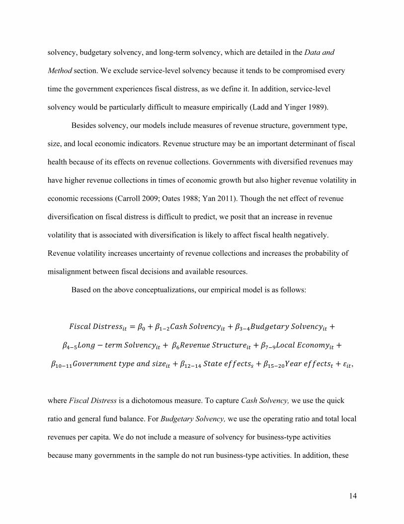
Based on the above conceptualizations, our empirical model is as follows:

!"#$%&("#)*+##,- = /0 + /2345%#ℎ78&9+:$;,- + /<3=>?@A+)%*;78&9+:$;,- +

/=3BC8:A − )+*E78&9+:$;,- +/FG+9+:?+7)*?$)?*+,- + /H3IC8$%&J$8:8E;,- +

/20322K89+*:E+:));L+%:@#"M+,- + /2432=7)%)++NN+$)#O + /2B340P+%*+NN+$)#- + Q,-,

where Fiscal Distress is a dichotomous measure. To capture Cash Solvency, we use the quick

ratio and general fund balance. For Budgetary Solvency, we use the operating ratio and total local

revenues per capita. We do not include a measure of solvency for business-type activities

because many governments in the sample do not run business-type activities. In addition, these

15

operations are typically self-funding and are unlikely to cause fiscal distress for a general

government. Long-term Solvency is measured as the level of debt and annual contributions to the

pension plans. Revenue Structure captures a share of own-source revenues coming from the

property tax. The models also control for government type and size and for local economic

factors such as the change in income, the change in housing prices, and the change in population.

To study the determinants of fiscal distress, we run binary logistic regression models with state

and year fixed effects. Since the observation period is only six years and the sample of

governments is relatively small, we focus on the models with heteroscedasticity-robust standard

errors clustered by city or county. We prefer these models to government fixed-effect models

that would involve the loss of multiple degrees of freedom and statistical power.

Data and Method

The variables for the analysis come from the following data sources: Comprehensive Annual

Financial Reports, budgets, news coverage, the US Census Bureau Annual Survey of

Government Finances, and Zillow, an online real-estate database company. Initially, we

collected CAFR data for 300 city and county governments from California, Pennsylvania, and

Michigan over the years 2007–2012, producing a panel of 1,800 observations. The sample

decreased to 1,767 observations after it was merged with the data from the US Census Bureau

Annual Survey of Government Finances. Our concern at the beginning of the project was that we

might not find enough cases of fiscal distress to run statistical models. We therefore selected

three states known for having high-profile cases of municipal fiscal distress (Stockton,

California; San Bernardino, California; Detroit, Michigan; Flint, Michigan; Harrisburg,

Pennsylvania; and Scranton, Pennsylvania).

16

As mentioned previously, we created the dependent variable through the analysis of

comprehensive annual financial reports, budgets, and news coverage. We operationalized fiscal

distress as actions, often disruptive and politically unpopular, that a government takes because it

is unable to meet its fundamental operating needs and service requirements. We coded a

government as fiscally distressed in a given year if its financial management was characterized

by at least one of the following: a blanket prohibition of overtime, a blanket reduction of

employee salaries, personnel furloughs or layoffs, deferral of payments to vendors and other

payees, large across-the-board budget cuts or cuts in key services, budget enactment later than

two months after the beginning of the fiscal year, pension contributions less than 75 percent of

annual required contributions, unusually large interfund transfers, unusual tax rate or fee

increases, declaration of fiscal emergency, default on municipal debt, credit rating downgrade,

bankruptcy, auditor doubts that the entity may continue to be a “going concern,” or a takeover by

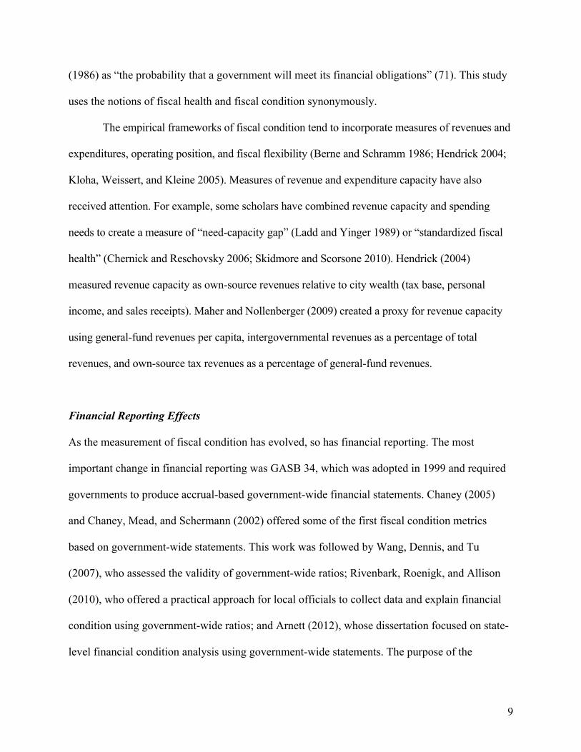
the state or significant state financial assistance (bailout). Table 1 provides frequencies of the

episodes of fiscal distress by state.

The explanatory variables are measured and scaled as follows:

• Cash solvency. The quick ratio consists of cash and cash equivalents divided by

current liabilities. The general fund balance is measured as a percentage of total

general fund expenditures.

• Budgetary solvency. The operating ratio is the ratio of total governmental funds revenues

to total governmental funds expenditures, expressed as a percentage. Total revenues per

capita are measured in thousands of dollars and adjusted for inflation using the Consumer

Price Index with 2012 as the base year.

17

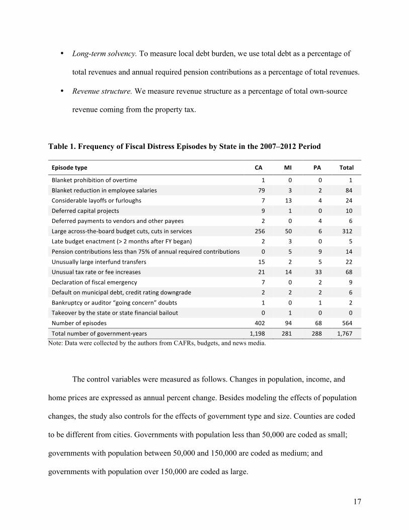
• Long-term solvency. To measure local debt burden, we use total debt as a percentage of

total revenues and annual required pension contributions as a percentage of total revenues.

• Revenue structure. We measure revenue structure as a percentage of total own-source

revenue coming from the property tax.

Table 1. Frequency of Fiscal Distress Episodes by State in the 2007–2012 Period

Episodetype CA MI PA Total

Blanketprohibitionofovertime 1 0 0 1Blanketreductioninemployeesalaries 79 3 2 84Considerablelayoffsorfurloughs 7 13 4 24Deferredcapitalprojects 9 1 0 10Deferredpaymentstovendorsandotherpayees 2 0 4 6Largeacross-the-boardbudgetcuts,cutsinservices 256 50 6 312Latebudgetenactment(>2monthsafterFYbegan) 2 3 0 5Pensioncontributionslessthan75%ofannualrequiredcontributions 0 5 9 14Unusuallylargeinterfundtransfers 15 2 5 22Unusualtaxrateorfeeincreases 21 14 33 68Declarationoffiscalemergency 7 0 2 9Defaultonmunicipaldebt,creditratingdowngrade 2 2 2 6Bankruptcyorauditor“goingconcern”doubts 1 0 1 2Takeoverbythestateorstatefinancialbailout 0 1 0 0Numberofepisodes 402 94 68 564Totalnumberofgovernment-years 1,198 281 288 1,767

Note: Data were collected by the authors from CAFRs, budgets, and news media.

The control variables were measured as follows. Changes in population, income, and

home prices are expressed as annual percent change. Besides modeling the effects of population

changes, the study also controls for the effects of government type and size. Counties are coded

to be different from cities. Governments with population less than 50,000 are coded as small;

governments with population between 50,000 and 150,000 are coded as medium; and

governments with population over 150,000 are coded as large.

18

Results

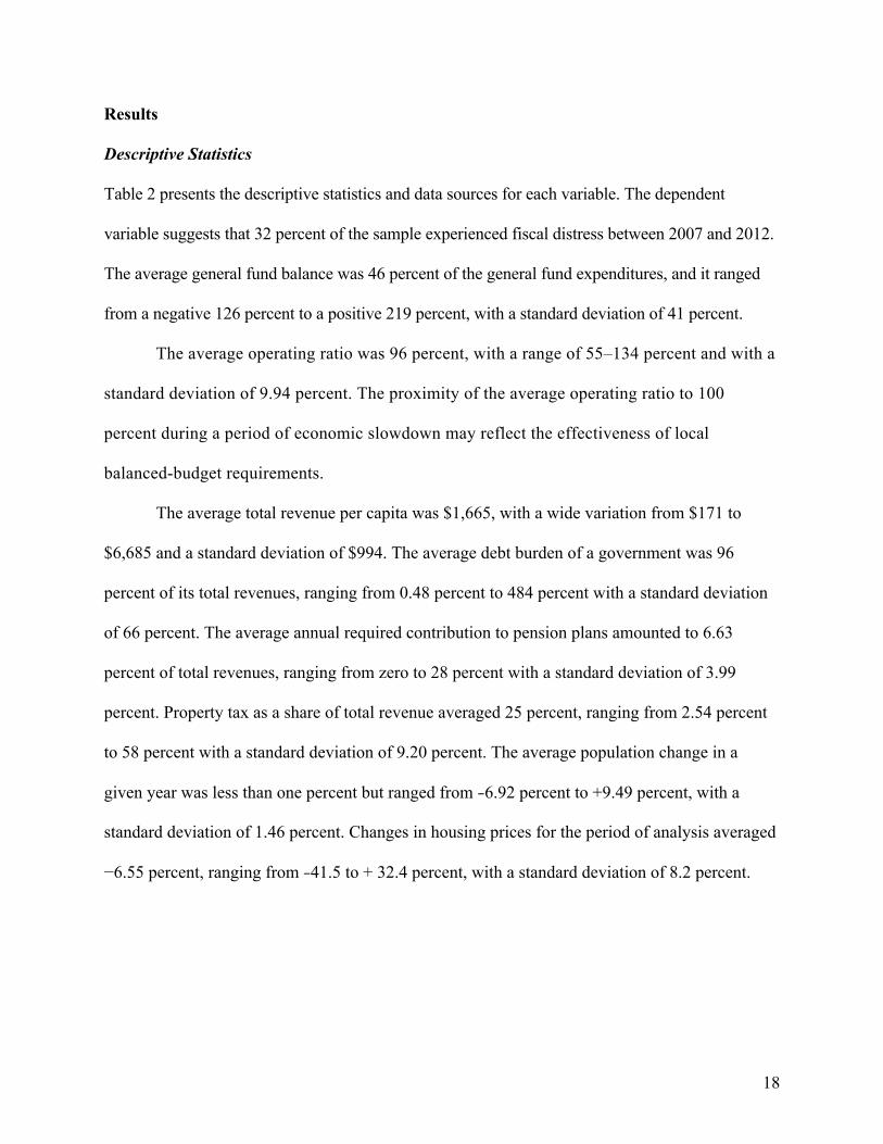
Descriptive Statistics

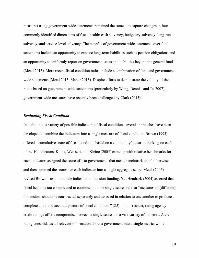
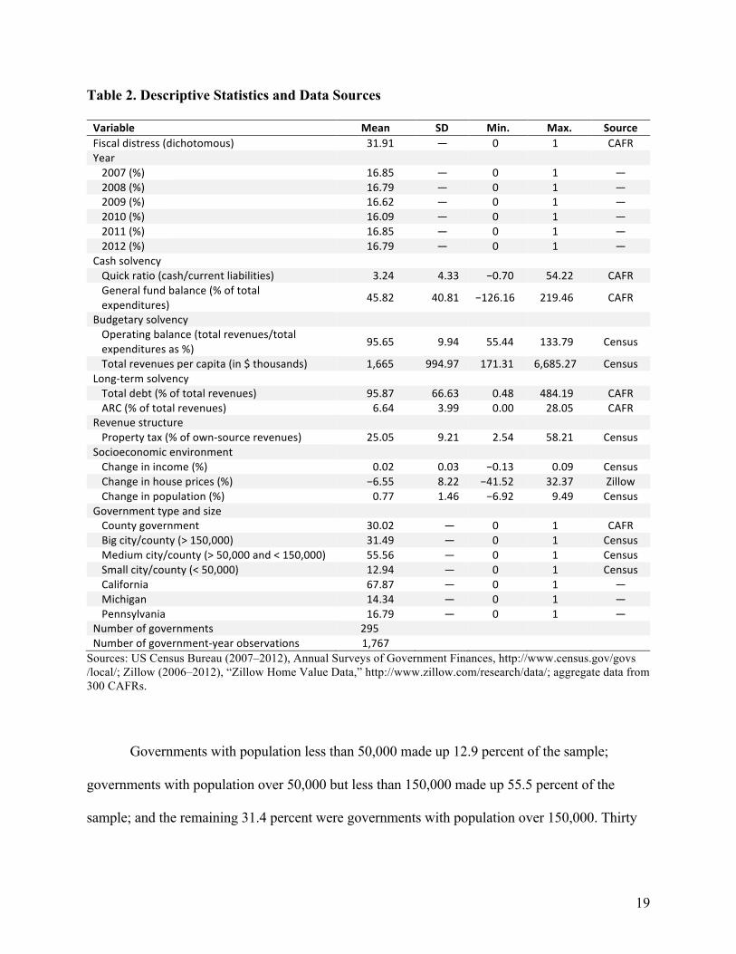
Table 2 presents the descriptive statistics and data sources for each variable. The dependent

variable suggests that 32 percent of the sample experienced fiscal distress between 2007 and 2012.

The average general fund balance was 46 percent of the general fund expenditures, and it ranged

from a negative 126 percent to a positive 219 percent, with a standard deviation of 41 percent.

The average operating ratio was 96 percent, with a range of 55–134 percent and with a

standard deviation of 9.94 percent. The proximity of the average operating ratio to 100

percent during a period of economic slowdown may reflect the effectiveness of local

balanced-budget requirements.

The average total revenue per capita was $1,665, with a wide variation from $171 to

$6,685 and a standard deviation of $994. The average debt burden of a government was 96

percent of its total revenues, ranging from 0.48 percent to 484 percent with a standard deviation

of 66 percent. The average annual required contribution to pension plans amounted to 6.63

percent of total revenues, ranging from zero to 28 percent with a standard deviation of 3.99

percent. Property tax as a share of total revenue averaged 25 percent, ranging from 2.54 percent

to 58 percent with a standard deviation of 9.20 percent. The average population change in a

given year was less than one percent but ranged from −6.92 percent to +9.49 percent, with a

standard deviation of 1.46 percent. Changes in housing prices for the period of analysis averaged

−6.55 percent, ranging from −41.5 to + 32.4 percent, with a standard deviation of 8.2 percent.

19

Table 2. Descriptive Statistics and Data Sources

Variable Mean SD Min. Max. SourceFiscaldistress(dichotomous) 31.91 — 0 1 CAFRYear 2007(%) 16.85 — 0 1 —2008(%) 16.79 — 0 1 —2009(%) 16.62 — 0 1 —2010(%) 16.09 — 0 1 —2011(%) 16.85 — 0 1 —2012(%) 16.79 — 0 1 —

Cashsolvency Quickratio(cash/currentliabilities) 3.24 4.33 −0.70 54.22 CAFRGeneralfundbalance(%oftotalexpenditures) 45.82 40.81 −126.16 219.46 CAFR

Budgetarysolvency Operatingbalance(totalrevenues/totalexpendituresas%) 95.65 9.94 55.44 133.79 Census

Totalrevenuespercapita(in$thousands) 1,665 994.97 171.31 6,685.27 CensusLong-termsolvency Totaldebt(%oftotalrevenues) 95.87 66.63 0.48 484.19 CAFRARC(%oftotalrevenues) 6.64 3.99 0.00 28.05 CAFR

Revenuestructure Propertytax(%ofown-sourcerevenues) 25.05 9.21 2.54 58.21 Census

Socioeconomicenvironment Changeinincome(%) 0.02 0.03 −0.13 0.09 CensusChangeinhouseprices(%) −6.55 8.22 −41.52 32.37 ZillowChangeinpopulation(%) 0.77 1.46 −6.92 9.49 Census

Governmenttypeandsize Countygovernment 30.02 — 0 1 CAFRBigcity/county(>150,000) 31.49 — 0 1 CensusMediumcity/county(>50,000and<150,000) 55.56 — 0 1 CensusSmallcity/county(<50,000) 12.94 — 0 1 CensusCalifornia 67.87 — 0 1 —Michigan 14.34 — 0 1 —Pennsylvania 16.79 — 0 1 —

Numberofgovernments 295 Numberofgovernment-yearobservations 1,767

Sources: US Census Bureau (2007–2012), Annual Surveys of Government Finances, http://www.census.gov/govs /local/; Zillow (2006–2012), “Zillow Home Value Data,” http://www.zillow.com/research/data/; aggregate data from 300 CAFRs.

Governments with population less than 50,000 made up 12.9 percent of the sample;

governments with population over 50,000 but less than 150,000 made up 55.5 percent of the

sample; and the remaining 31.4 percent were governments with population over 150,000. Thirty

20

percent of the sample were counties. Over two-thirds of the cities and counties were in California,

roughly 14 percent were in Michigan, and the remaining 16 percent were in Pennsylvania.

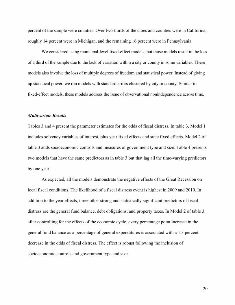
We considered using municipal-level fixed-effect models, but those models result in the loss

of a third of the sample due to the lack of variation within a city or county in some variables. These

models also involve the loss of multiple degrees of freedom and statistical power. Instead of giving

up statistical power, we run models with standard errors clustered by city or county. Similar to

fixed-effect models, these models address the issue of observational nonindependence across time.

Multivariate Results

Tables 3 and 4 present the parameter estimates for the odds of fiscal distress. In table 3, Model 1

includes solvency variables of interest, plus year fixed effects and state fixed effects. Model 2 of

table 3 adds socioeconomic controls and measures of government type and size. Table 4 presents

two models that have the same predictors as in table 3 but that lag all the time-varying predictors

by one year.

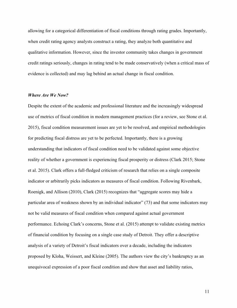
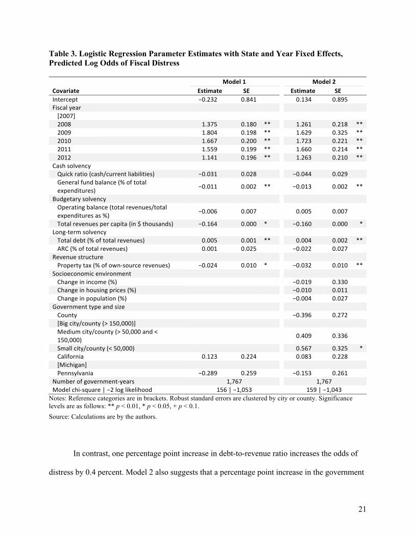
As expected, all the models demonstrate the negative effects of the Great Recession on

local fiscal conditions. The likelihood of a fiscal distress event is highest in 2009 and 2010. In

addition to the year effects, three other strong and statistically significant predictors of fiscal

distress are the general fund balance, debt obligations, and property taxes. In Model 2 of table 3,

after controlling for the effects of the economic cycle, every percentage point increase in the

general fund balance as a percentage of general expenditures is associated with a 1.3 percent

decrease in the odds of fiscal distress. The effect is robust following the inclusion of

socioeconomic controls and government type and size.

21

Table 3. Logistic Regression Parameter Estimates with State and Year Fixed Effects, Predicted Log Odds of Fiscal Distress Model1 Model2Covariate Estimate SE Estimate SE Intercept −0.232 0.841 0.134 0.895 Fiscalyear [2007] 2008 1.375 0.180 ** 1.261 0.218 **2009 1.804 0.198 ** 1.629 0.325 **2010 1.667 0.200 ** 1.723 0.221 **2011 1.559 0.199 ** 1.660 0.214 **2012 1.141 0.196 ** 1.263 0.210 **

Cashsolvency Quickratio(cash/currentliabilities) −0.031 0.028 −0.044 0.029 Generalfundbalance(%oftotalexpenditures) −0.011 0.002 ** −0.013 0.002 **

Budgetarysolvency Operatingbalance(totalrevenues/totalexpendituresas%) −0.006 0.007 0.005 0.007

Totalrevenuespercapita(in$thousands) −0.164 0.000 * −0.160 0.000 *Long-termsolvency Totaldebt(%oftotalrevenues) 0.005 0.001 ** 0.004 0.002 **ARC(%oftotalrevenues) 0.001 0.025 −0.022 0.027

Revenuestructure Propertytax(%ofown-sourcerevenues) −0.024 0.010 * −0.032 0.010 **

Socioeconomicenvironment Changeinincome(%) −0.019 0.330 Changeinhousingprices(%) −0.010 0.011 Changeinpopulation(%) −0.004 0.027

Governmenttypeandsize County −0.396 0.272 [Bigcity/county(>150,000)] Mediumcity/county(>50,000and<150,000) 0.409 0.336

Smallcity/county(<50,000) 0.567 0.325 *California 0.123 0.224 0.083 0.228 [Michigan] Pennsylvania −0.289 0.259 −0.153 0.261

Numberofgovernment-years 1,767 1,767Modelchi-square|−2loglikelihood 156|−1,053 159|−1,043

Notes: Reference categories are in brackets. Robust standard errors are clustered by city or county. Significance levels are as follows: ** p < 0.01, * p < 0.05, + p < 0.1. Source: Calculations are by the authors.

In contrast, one percentage point increase in debt-to-revenue ratio increases the odds of

distress by 0.4 percent. Model 2 also suggests that a percentage point increase in the government

22

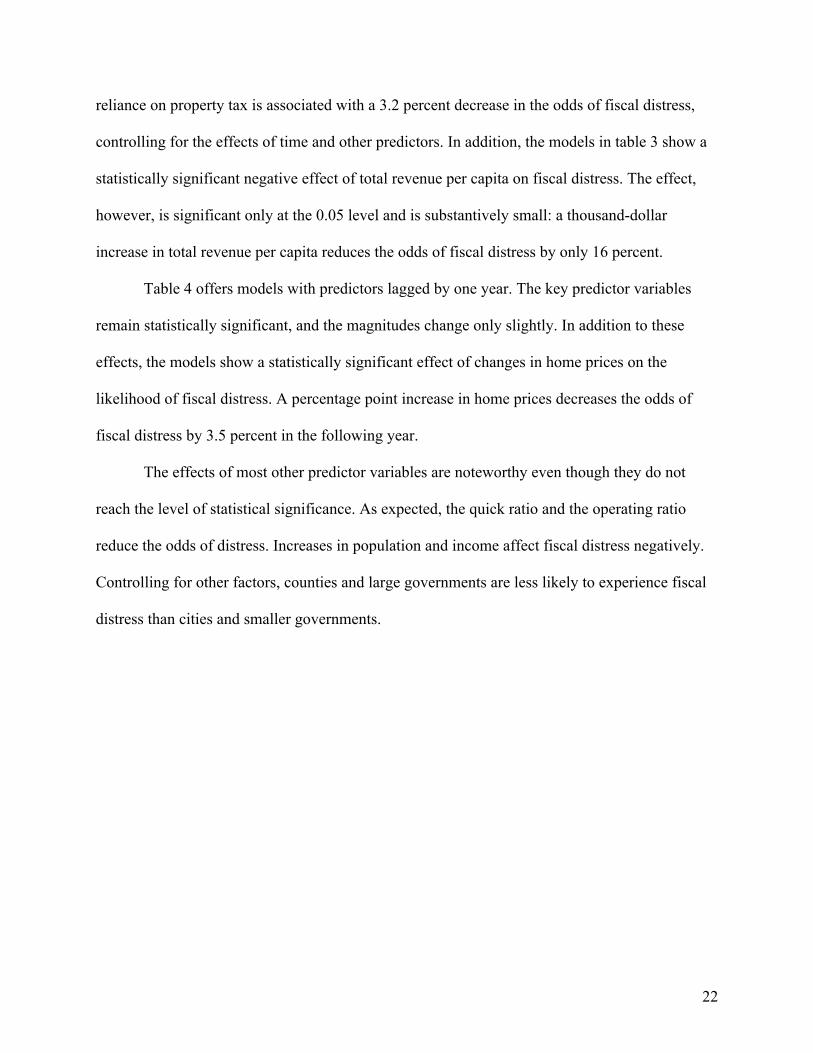
reliance on property tax is associated with a 3.2 percent decrease in the odds of fiscal distress,

controlling for the effects of time and other predictors. In addition, the models in table 3 show a

statistically significant negative effect of total revenue per capita on fiscal distress. The effect,

however, is significant only at the 0.05 level and is substantively small: a thousand-dollar

increase in total revenue per capita reduces the odds of fiscal distress by only 16 percent.

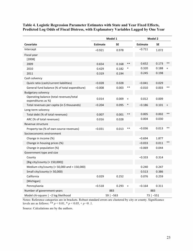
Table 4 offers models with predictors lagged by one year. The key predictor variables

remain statistically significant, and the magnitudes change only slightly. In addition to these

effects, the models show a statistically significant effect of changes in home prices on the

likelihood of fiscal distress. A percentage point increase in home prices decreases the odds of

fiscal distress by 3.5 percent in the following year.

The effects of most other predictor variables are noteworthy even though they do not

reach the level of statistical significance. As expected, the quick ratio and the operating ratio

reduce the odds of distress. Increases in population and income affect fiscal distress negatively.

Controlling for other factors, counties and large governments are less likely to experience fiscal

distress than cities and smaller governments.

23

Table 4. Logistic Regression Parameter Estimates with State and Year Fixed Effects, Predicted Log Odds of Fiscal Distress, with Explanatory Variables Lagged by One Year

Model1 Model2

Covariate Estimate SE Estimate SE Intercept −0.921 0.978 −0.711 1.072

Fiscalyear

[2008]

2009 0.654 0.168 ** 0.652 0.173 **

2010 0.429 0.182 * 0.320 0.188 +

2011 0.319 0.194 0.245 0.198

Cashsolvency Quickratio(cash/currentliabilities) −0.028 0.028 −0.041 0.029 Generalfundbalance(%oftotalexpenditure) −0.008 0.003 ** -0.010 0.003 **

Budgetarysolvency Operatingbalance(totalrevenues/totalexpendituresas%) 0.014 0.009 + 0.012 0.009

Totalrevenuespercapita(in$thousands) −0.204 0.095 * −0.186 0.101 +Long-termsolvency

Totaldebt(%oftotalrevenues) 0.007 0.001 ** 0.005 0.002 **

ARC(%oftotalrevenues) 0.016 0.028 0.004 0.030

Revenuestructure Propertytax(%ofown-sourcerevenues) −0.031 0.013 ** −0.036 0.013 **

Socioeconomicenvironment

Changeinincome(%) −0.694 1.877

Changeinhousingprices(%) −0.033 0.011 **

Changeinpopulation(%) −0.069 0.044

Governmenttypeandsize County −0.333 0.314 [Bigcity/county(>150,000)] Mediumcity/county(>50,000and<150,000) 0.240 0.247 Smallcity/county(<50,000) 0.513 0.386 California 0.029 0.252 0.076 0.259 [Michigan] Pennsylvania −0.518 0.293 + −0.164 0.311

Numberofgovernment-years 883 883Modelchi-square|−2loglikelihood 59|−563 73|−551

Notes: Reference categories are in brackets. Robust standard errors are clustered by city or county. Significance levels are as follows: ** p < 0.01, * p < 0.05, + p <0 .1. Source: Calculations are by the authors.

24

Discussion and Conclusion

As stated earlier, 32 percent of the communities across the three states in our sample experienced

fiscal distress, which, on its own, sheds light on the magnitude of the 2007–2009 recession.

Understanding the determinants of those incidents has been the focus of a number of scholars for

more than 40 years. This study has taken a novel approach to the measurement and prediction of

fiscal condition. Rather than trying to define fiscal stress through a set of fiscal and

environmental indicators (e.g., Brown 1993; Kloha, Weissert, and Kleine 2005; Mead 2006), we

identified local fiscal distress based on the analysis of governmental actions that indicated

difficulties in maintaining a healthy fiscal path. We then tested theoretically grounded

parsimonious models to best predict the incidents of fiscal distress.

While not offering the explanatory power we would have preferred (pseudo R2 range

from 0.05 to 0.12), our models do offer insights into factors that are associated with fiscal

distress in communities. We conclude that a reduction in the level of local fiscal reserves is a

strong predictor of fiscal trouble and that an increase in debt as a share of total revenue increases

the odds of fiscal distress. The findings, while not novel, highlight the importance of basic

budgeting principles and should generate policy conversations at the local level about the

appropriate size of fund balance and appropriate debt levels.

Importantly, local reliance on property tax revenues is negatively associated with fiscal

distress. This finding suggests that communities that are relatively more reliant on non–property

tax revenues expose themselves to a higher likelihood of fiscal distress in a recession than

governments that are more reliant on the property tax. Interestingly, due to its unique nature—the

housing bubble and burst—the 2007–2009 recession had dramatic effects on property taxes. The

models show that local governments reliant on property taxes managed to weather the recession

25

better than governments reliant on other revenue sources. Importantly, given the lagged effects

of the recession on property assessment values, decreases in property tax collection happened

only after the recession had passed. By the time property assessments caught up with the declines

in home market values, local sales taxes as well as fees and charges, which had been hit hard by

economic contraction, had already begun to rebound. Even though the regression results caution

governments against a heavy reliance on income-elastic revenue sources, governments need not

necessarily scale down their revenue diversification strategies. Instead, after recognizing the risk

that diversification poses to local fiscal health over the economic cycle, local officials could look

for ways to guard against this additional risk—for example, by holding higher fiscal reserves or

by arranging with other governments or the private sector for quick access to cash in a

recessionary period.

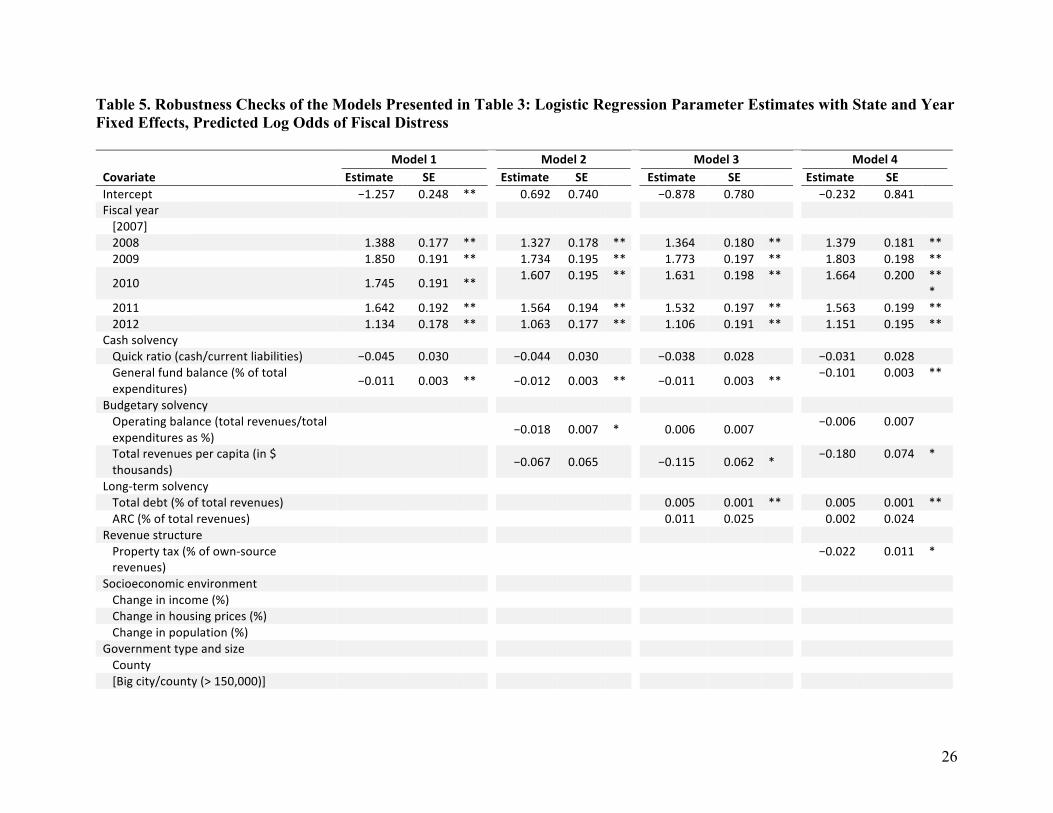
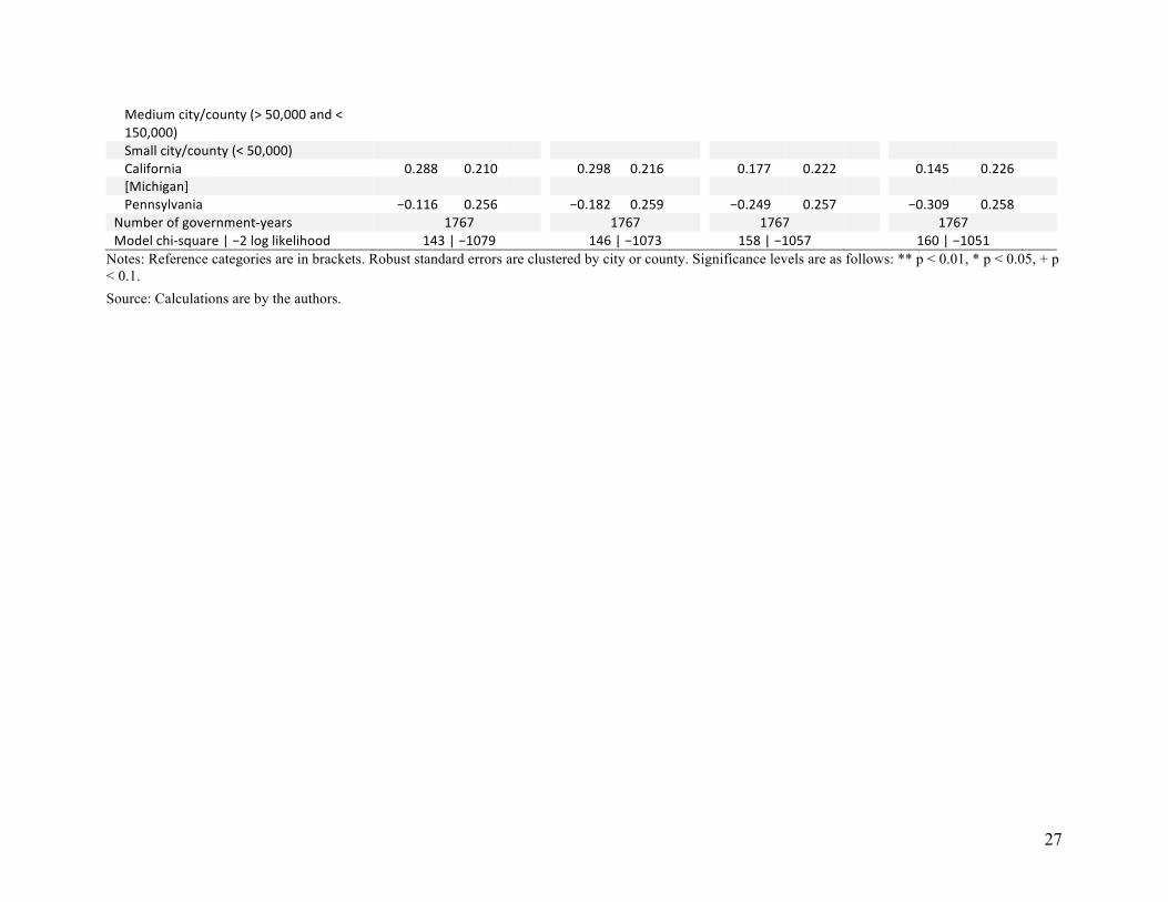
We present additional models in table 5. Before running the models, we conducted

diagnostics of all independent variables to make sure that their distributions were appropriate for

running the models. We tried removing outliers and using logarithms for all the variables with non-

normal distributions as part of the robustness testing. The results did not change much, and we

decided to keep the independent variables consistent. All of them are expressed as percentages.

26

Table 5. Robustness Checks of the Models Presented in Table 3: Logistic Regression Parameter Estimates with State and Year Fixed Effects, Predicted Log Odds of Fiscal Distress Model1 Model2 Model3 Model4Covariate Estimate SE Estimate SE Estimate SE Estimate SE Intercept −1.257 0.248 ** 0.692 0.740 −0.878 0.780 −0.232 0.841 Fiscalyear [2007] 2008 1.388 0.177 ** 1.327 0.178 ** 1.364 0.180 ** 1.379 0.181 **2009 1.850 0.191 ** 1.734 0.195 ** 1.773 0.197 ** 1.803 0.198 **

2010 1.745 0.191 ** 1.607 0.195 ** 1.631 0.198 ** 1.664 0.200 ***

2011 1.642 0.192 ** 1.564 0.194 ** 1.532 0.197 ** 1.563 0.199 **2012 1.134 0.178 ** 1.063 0.177 ** 1.106 0.191 ** 1.151 0.195 **

Cashsolvency Quickratio(cash/currentliabilities) −0.045 0.030 −0.044 0.030 −0.038 0.028 −0.031 0.028 Generalfundbalance(%oftotalexpenditures) −0.011 0.003 ** −0.012 0.003 ** −0.011 0.003 ** −0.101 0.003 **

Budgetarysolvency Operatingbalance(totalrevenues/totalexpendituresas%) −0.018 0.007 * 0.006 0.007 −0.006 0.007

Totalrevenuespercapita(in$thousands) −0.067 0.065 −0.115 0.062 * −0.180 0.074 *

Long-termsolvency Totaldebt(%oftotalrevenues) 0.005 0.001 ** 0.005 0.001 **ARC(%oftotalrevenues) 0.011 0.025 0.002 0.024

Revenuestructure Propertytax(%ofown-sourcerevenues) −0.022 0.011 *

Socioeconomicenvironment Changeinincome(%) Changeinhousingprices(%) Changeinpopulation(%)

Governmenttypeandsize County [Bigcity/county(>150,000)]

27

Mediumcity/county(>50,000and<150,000)

Smallcity/county(<50,000) California 0.288 0.210 0.298 0.216 0.177 0.222 0.145 0.226 [Michigan] Pennsylvania −0.116 0.256 −0.182 0.259 −0.249 0.257 −0.309 0.258

Numberofgovernment-years 1767 1767 1767 1767 Modelchi-square|−2loglikelihood 143|−1079 146|−1073 158|−1057 160|−1051

Notes: Reference categories are in brackets. Robust standard errors are clustered by city or county. Significance levels are as follows: ** p < 0.01, * p < 0.05, + p < 0.1. Source: Calculations are by the authors.

28

In summary, our models show a relatively pronounced role of fiscal reserves, debt, and

revenue structure in the prediction of local fiscal distress. This study highlights the importance of

local fiscal policy that focuses on building and using adequate fiscal reserves to weather fiscal

shocks. This policy is even more salient today than in previous decades because of the state-level

initiatives to limit local taxing authority, especially property taxes in the vein of California’s

Proposition 13 and efforts to impose limits on revenue growth in the vein of Colorado’s

Taxpayer Bill of Rights, which by definition limit a community’s ability to grow reserves. In

addition, revenue diversification also calls for a responsible fiscal reserves policy because, while

generally positive, it also means that governments need to be better prepared for fiscal shocks as

their revenue structures become more vulnerable.

Lastly, these findings may be generalized only with caution. As previously stated, the Great

Recession was unlike any other recession seen in the recent past. The housing bubble-burst resulted

in a unique level of fiscal distress. Similarly, many local governments, especially in California and

Michigan, were hit particularly hard during the recession for different reasons—housing bubble-

burst in California and long-term fiscal distress in Michigan—meaning that the generalizability of

the results to local governments throughout the United States is limited until the research can be

expanded beyond these two states. Since the predictive power of individual measures of solvency

and revenue structure is relatively modest, future research should consider exploring interactions

between these individual measures of solvency as predictors of fiscal distress.

29

References

ACIR (Advisory Commission on Intergovernmental Relations). 1971. Measuring the Fiscal Capacity and Effort of State and Local Areas. Washington, DC: US Government Printing Office.

———. 1979. State-Local Finances in Recession and Inflation: An Economic Analysis.

Washington, DC: US Government Printing Office. ———. 1981. Measuring Local Discretionary Authority. Washington, DC: US Government

Printing Office. ———. 1988. Local Revenue Diversification: Local Income Taxes. Washington, DC: US

Government Printing Office. ———. 1989. Local Revenue Diversification: Local Sales Taxes. Washington, DC: US

Government Printing Office. Arnett, S. 2012. “Fiscal Stress in the U.S. States: An Analysis of Measures and Responses.” PhD

diss., Georgia State University, 2012. http://scholarworks.gsu.edu/pmap_diss/38. Berne, R., and R. Schramm. 1986. The Financial Analysis of Governments. Englewood Cliffs,

NJ: Prentice-Hall. Brown, K. W. 1993. “Ten-Point Test of Financial Condition: Toward an Easy-to-Use

Assessment Tool for Small Cities.” Government Finance Review 9 (6): 21–26. Carroll, D. A. 2009. “Diversifying Municipal Government Revenue Structures: Fiscal Illusion or

Instability?” Public Budgeting & Finance 29 (1): 27–48. Chaney, B. 2005. “Analyzing the Financial Condition of the City of Corona, California: Using a

Case to Teach the GASB 34 Government-Wide Financial Statements.” Journal of Public Budgeting, Accounting and Financial Management 17 (2): 180–201.

Chaney, B., D. M. Mead, and K. Schermann. 2002. “The New Governmental Financial

Reporting Model.” Journal of Government Financial Management 51 (1): 26–31. Chapman, J. A. 2008. “State and Local Fiscal Sustainability: The Challenges.” Public

Administration Review 68 (S1): S115–S131. Chernick, H., and A. Reschovsky. 2006. “Fiscal Conditions in Selected Metropolitan Areas.” La

Follette School Working Paper No. 2006-010, Robert M. LaFollette School of Public Affairs, Madison, WI. http://www.lafollette.wisc.edu/images/publications/workingpapers /reschovsky2006-011.pdf.

30

Clark, B. Y. 2015. “Evaluating the Validity and Reliability of the Financial Condition Index for Local Governments.” Public Budgeting and Finance 35 (2): 66–88.

Clark, T. N., and Ferguson, L. C. 1983. City Money: Political Processes, Fiscal Strain, and

Retrenchment. New York: Columbia University Press. Coe, C. 2007. “Preventing Local Government Fiscal Crises: The North Carolina Approach.”

Public Budgeting and Finance 27 (3): 39–49. Convery, A., and A. J. Imdieke. 2015. “The Effectiveness of Setting Governmental Accounting

Standards: The Case of Michigan Governments in Fiscal Distress.” Mercatus Working Paper, Mercatus Center at George Mason University, Arlington, VA.

Crosby, A., and D. Robbins. 2013. “Mission Impossible: Monitoring Municipal Fiscal

Sustainability and Stress in Michigan.” Journal of Public Budgeting, Accounting and Financial Management 25 (3): 522–35.

Frank, H. A. 2006. Public Financial Management. Boca Raton, FL: Taylor and Francis. Groves, S. M., and M. G. Valente. 1986. Evaluating Financial Condition: A Handbook for Local

Government. Washington, DC: International City/County Management Association. ———. 1994. Evaluating Financial Condition: A Handbook for Local Government, 3rd ed.

Washington, DC: International City/County Management Association. Hendrick, R. 2004. “Assessing and Measuring the Fiscal Health of Local Governments: Focus on

Chicago Metropolitan Suburbs.” Urban Affairs Review 40 (1): 78–114. ———. 2011. Managing the Fiscal Metropolis: The Financial Policies, Practices, and Health of

Suburban Municipalities. Washington, DC: Georgetown University Press. Hoene, C., and M. Pagano. 2009. “City Fiscal Conditions in 2009.” Research Brief on America’s

Cities. Washington, DC: National League of Cities. http://www.nlc.org/documents/Find %20City%20Solutions/Research%20Innovation/Finance/city-fiscal-conditions-2009-rpt -sep09.pdf.

Honadle, B., J. Costa, and B. Cigler. 2004. Fiscal Health for Local Governments: An

Introduction to Concepts, Practical Analysis, and Strategies. San Diego, CA: Elsevier Academic Press.

Jacob, B., and R. Hendrick. 2013. “Assessing the Financial Condition of Local Governments:

What Is Financial Condition and How Is It Measured?” In Handbook of Local Government Fiscal Health, edited by H. Levine, J. B. Justice, and E. A. Scorsone. Burlington, MA: Jones and Bartlett Learning.

31

Justice, J., and E. Scorsone. 2013. “Measuring and Predicting Local Government Fiscal Stress: Theory and Practice.” In Handbook of Local Government Fiscal Health, edited by H. Levine, J. B. Justice, and E. A. Scorsone. Burlington, MA: Jones and Bartlett Learning.

Kloha, K., C. S. Weissert, and R. Kleine. 2005. “Developing and Testing a Composite Model to

Predict Local Fiscal Disparities.” Public Administration Review 65 (3): 313–23. Kravchuk, R. S., and S. B. Stone. 2010. “How and When Do Structural Deficits Reveal

Themselves? The Case of Indiana.” Journal of Public Budgeting, Accounting & Financial Management 22 (4): 487–510.

Ladd, H. F., and J. Yinger. 1989. America’s Ailing Cities: Fiscal Health and the Design of

Urban Policy. Baltimore, MD: Johns Hopkins University Press. Levine, H. C., I. S. Rubin, and G. Wolohojian. 1981. The Politics of Retrenchment: How Local

Governments Manage Fiscal Stress. Beverly Hills, CA: Sage Publications. Levine, H. C., J. B. Justice, and E. A. Scorsone, eds. 2013. Handbook of Local Government

Fiscal Health. Burlington, MA: Jones and Bartlett Learning. Maher, C. 2013. “Measuring Financial Condition: An Essential Element of Management during

Periods of Fiscal Stress.” Journal of Public Financial Management 61 (1): 20–25. Maher, C. S., and K. Nollenberger. 2009. “Revisiting Kenneth Brown’s 10-Point Test.”

Government Finance Review 25 (5): 61–66. Mead, D. 2006. “A Manageable System of Economic Condition Analysis for Governments.” In

Public Financial Management, edited by H. A. Frank. Boca Raton, FL: Taylor and Francis.

———. 2013. “The Development of External Financial Reporting and Its Relationship to the

Assessment of Fiscal Health and Stress.” In Handbook of Local Government Fiscal Health, edited by H. Levine, J. B. Justice, and E. A. Scorsone. Burlington, MA: Jones and Bartlett Learning.

Nollenberger, K., S. M. Groves, and M. G. Valente. 2003. Evaluating Financial Condition: A

Handbook for Local Government, 4th ed. Washington, DC: International City/County Management Association.

Oates, W. 1988. “On the Nature and Measurement of Fiscal Illusion: A Survey.” In Taxation and

Fiscal Federalism: Essays in Honour of Russell Mathews, edited by G. Brennan, B. Grewal, and P. Groenewegen. Sydney: Australian National University Press. http://econweb.umd.edu/~oates/research/On%20the%20Nature%20and%20Measurement%20of%20Fiscal%20Illusion.pdf.

32

Office of the New York State Comptroller. 2015. Financial Condition Report for Fiscal Year Ended March 31, 2015. Albany. http://www.osc.state.ny.us/finance/finreports/fcr /2015/fcrindex.htm.

Pammer, W. J. 1990. Managing Fiscal Strain in Major American Cities: Understanding

Retrenchment in the Public Sector. New York: Greenwood Press. Pennsylvania Department of Community and Economic Development. 2011. Financial

Monitoring Workbook, 3rd ed. Harrisburg. http://dced.pa.gov/download/financial -monitoring-workbook-2011-pdf-2/?wpdmdl=59422.

Plerhoples, C., and E. Scorsone. 2011. “Proposed Alterations to the Local Government Fiscal

Stress Indicator System for the State of Michigan.” Staff Paper Series 2011-03. East Lansing: Michigan State University. http://ageconsearch.umn.edu/bitstream/116167/2 /StaffPaper2011-03.pdf.

Rivenbark, W., D. Roenigk, and G. Allison. 2010. “Conceptualizing Financial Condition in

Local Government.” Journal of Public Budgeting, Accounting and Financial Management 22 (2): 149–77.

Rubin, I. S. 1982. Running in the Red: The Political Dynamics of Urban Fiscal Stress. Albany:

State University of New York Press. Scorsone, E. 2014. “Municipal Fiscal Emergency Laws: Background and Guide to State-Based

Approaches.” Mercatus Working Paper, Mercatus Center at George Mason University, Arlington, VA.

Skidmore, M., and E. Scorsone. 2010. “Causes and Consequences of Fiscal Stress in Michigan

Municipal Governments.” Regional Science and Urban Economics 41 (4): 360–71. Stone, S., A. Singla, J. Comeaux, and C. Kirschner. 2015. “A Comparison of Financial

Indicators: The Case of Detroit.” Public Budgeting and Finance 35 (4): 90–111. US Census Bureau. 2007–2012. Annual Surveys of Government Finances.

http://www.census.gov/govs/local/. Wang, X., L. Dennis, and Y. S. Tu. 2007. “Measuring Financial Condition: A Study of U.S.

States.” Public Budgeting and Finance 27 (1): 1–21. Yan, W. 2011. “The Interactive Effect of Revenue Diversification and Economic Base on US

Local Government Revenue Stability.” Public Money & Management 31 (6): 419–26. Zillow. 2006–2012. “Zillow Home Value Data.” http://www.zillow.com/research/data/.