Measuring and Modeling Variation in the Risk-Return

Tradeoff ∗

Martin Lettau

New York University, CEPR, NBER

Sydney C. Ludvigson

New York University and NBER

Preliminary

Comments Welcome

First draft: July 24, 2001

This draft: December 3, 2003

∗Lettau: Department of Finance, Stern School of Business, New York University, 44 West Fourth Street,New York, NY 10012-1126; Email: mlettau@stern.nyu.edu, Tel: (212) 998-0378; Fax: (212) 995-4233.Ludvigson: Department of Economics, New York University, 269 Mercer Street, 7th Floor, New York,NY 10003; Email: sydney.ludvigson@nyu.edu; Tel: (212) 998-8927; Fax: (212) 995-4186.This paper has been prepared for the Handbook of Financial Econometrics, edited by Yacine Ait-

Sahalia and Lars Peter Hansen. Updated versions, along with the data on cayt, may be found athttp://www.stern.nyu.edu/˜ mlettau and http://www.econ.nyu.edu/user/ludvigsons/. Lettau ac-knowledges financial support from the National Science Foundation; Ludvigson acknowledges financial sup-port from the Alfred P. Sloan Foundation and the National Science Foundation. We are grateful to MichaelBrandt, Rob Engle, Stijn Van Nieuwerburgh, and Jessica Wachter for helpful comments. Nathan Barczi andAdam Kolasinski provided excellent research assistance. Any errors or omissions are the responsibility ofthe authors.

Measuring and Modeling Variation in the Risk-Return Tradeoff

Abstract

Are excess stock market returns predictable over time and, if so, at what horizons and

with which economic indicators? Can stock return predictability be explained by changes

in stock market volatility? How does the mean return per unit risk change over time? This

chapter reviews what is known about the time-series evolution of the risk-return tradeoff for

stock market investment, and presents some new empirical evidence using a proxy for the log

consumption-aggregate wealth ratio as a predictor of both the mean and volatility of excess

stock market returns.

We characterize the risk-return tradeoff as the conditional expected excess return on a

broad stock market index divided by its conditional standard deviation, a quantity commonly

known as the Sharpe ratio. Our own investigation suggests that variation in the equity risk-

premium is strongly negatively linked to variation in market volatility, at odds with leading

asset pricing models. Since the conditional volatility and conditional mean move in opposite

directions, the degree of countercyclicality in the Sharpe ratio that we document here is

far more dramatic than that produced by existing equilibrium models of financial market

behavior, which completely miss the sheer magnitude of variation in the price of stock market

risk; leading asset pricing paradigms leave a “Sharpe ratio volatility puzzleÔ that remains to

be explained.

JEL: G10, G12.

1 Introduction

Financial markets are often hard to understand. Stock prices frequently seem volatile and

unpredictable, and researchers have devoted significant resources to understanding the be-

havior of expected returns relative to the risk of stock market investment. Are excess stock

market returns predictable over time and, if so, at what horizons and with which economic

indicators? Can stock return predictability be explained by changes in stock market volatil-

ity? How does the mean return per unit risk change over time? For academic researchers,

the progression of empirical evidence aimed at these questions has presented a continuing

challenge to asset pricing theory and an important road map for future inquiry. For many

investment professionals, finding practical answers to these questions is the fundamental

purpose of financial economics, as well as its principal reward.

Despite both the theoretical and practical importance of these issues, relatively little is

known about how the risk-return tradeoff varies over the business cycle or with key macroe-

conomic indicators. This chapter reviews the state of knowledge on such variation for stock

market investment, and presents some new empirical evidence based on information con-

tained in aggregate consumption and aggregate labor income. We define the risk-return

tradeoff as the conditional expected excess return on a broad stock market index divided by

its conditional standard deviation, a quantity commonly known as the Sharpe ratio. Our

study focuses not on the unconditional value of this ratio, but on its evolution through time.

Understanding the time-series properties of the Sharpe ratio is crucial to the development

of theoretical models capable of explaining observed patterns of stock market predictability

and volatility. For example, Hansen and Jagannathan (1991) showed that the maximum

value of the Sharpe ratio places restrictions on the volatility of the set of discount factors

that can be used to price returns. The same reasoning implies that the pattern of time-

series variation in the Sharpe ratio will also place restrictions on the set of discount factors

capable of pricing equity returns. In addition, the behavior of the Sharpe ratio over time

is fundamental for assessing whether stocks are safer in the long run than they are in the

short run, as increasingly advocated by popular guides to investment strategy (e.g., Siegel

(1998)). Only if the Sharpe ratio grows more quickly than the square root of the horizon–so

that the variance of the return grows more slowly than its mean–are stocks safer investments

in the long run than they are in the short run. Such a dynamic pattern is not possible if

stock returns are unpredictable, i.i.d. random variables. Thus, understanding the time-series

behavior of the Sharpe ratio not only provides a benchmark for theoretical progress, it has

3

profound implications for investment professionals concerned with strategic asset allocation.

The two components of the risk-return relation (the numerator and the denominator of

the Sharpe ratio) are the conditional mean excess stock return, and the conditional standard

deviation of the excess return. We focus here on empirically measuring and statistically

modeling each of these components separately, a process that can be unified to reveal an

estimate of the conditional Sharpe ratio, or price of stock market risk. Section 2 discusses

estimation of the conditional mean of excess stock returns. In this section we evaluate the

statistical evidence for stock return predictability and review the range of indicators with

which such predictability has been associated. Taken together, this evidence suggests that

excess returns on broad stock market indexes are predictable at long-horizons, implying that

the reward for bearing risk varies over time.

One possible explanation for time-variation in the equity risk premium is time variation

in stock market volatility. Section 3 reviews the evidence for time-variation in stock market

volatility. In many classic asset pricing models, the equity risk premium varies proportionally

with stock market volatility. These models require that periods of high excess stock returns

coincide with periods of high stock market volatility, implying a constant price of risk. It

follows that variation in the equity risk premium must be perfectly positively correlated with

variation in stock market volatility.

The important empirical question is whether such a positive correlation between the

mean and volatility of returns exists, implying a constant Sharpe ratio. Section 4 ties the

evidence on the conditional mean of excess returns in with that on the conditional variance

to derive implications for the time-series behavior of the conditional Sharpe ratio. Existing

empirical evidence on the sign of the relationship between the conditional mean and the

conditional volatility of excess stock returns is mixed and somewhat weak. This may be

because some studies have relied on parametric or semi-parametric ARCH-like models of

volatility that impose a relatively high degree of structure about which there is little direct

empirical evidence. Others have used predictive variables for volatility that are only weakly

related to the first moments of returns, and vice versa. Finally, it has been difficult to explain

high risk premia with high volatility because evidence suggests that returns are predicable

at quarterly and longer horizons, while variation in stock market volatility has, to date, been

most evident in high frequency (e.g., daily) data.

In addition to reviewing existing evidence, this chapter presents some new evidence on

the risk-return tradeoff. We find that a proxy for the log consumption-aggregate wealth ratio,

a variable shown elsewhere to predict excess returns and constructed using information on

4

aggregate consumption and labor income, is also a strong predictor of stock market volatility.

These findings differ from existing evidence because they reveal the presence of at least one

observable conditioning variable that strongly forecasts both the mean and volatility of

returns. Moreover, these results show that the evidence for changing stock market risk is

not confined to high frequency data: stock market volatility is forecastable over horizons

ranging from one quarter to six years.

These findings imply that movements in the equity risk-premium are linked empirically

to stock market volatility. In addition, the predictability patterns we find for excess returns

and volatility imply pronounced countercyclical variation in the Sharpe ratio. This evidence

weighs against many time-honored asset pricing models that specify a constant price of risk

(for example, the static capital asset pricing model (CAPM) of Sharpe (1964) and Lintner

(1965)), and toward more recent paradigms capable of rationalizing a countercyclical Sharpe

ratio (e.g., Campbell and Cochrane (1999); Barberis, Huang, and Santos (2001)). Although

these more recent frameworks imply a positive correlation between the conditional mean

and conditional volatility of returns, unlike the classic asset pricing models this positive

correlation is not perfect, making countercyclical variation in the Sharpe ratio possible.

Yet despite evidence that the Sharpe ratio varies countercyclically, our results neverthe-

less present a problem for modern-day asset pricing theory. Instead of finding a positive

correlation between the condition mean and conditional volatility, we find a strong negative

correlation, consistent with the findings of a number of other studies discussed below. More

significantly, since the conditional volatility and conditional mean move in opposite direc-

tions, the magnitude of countercyclicality in the Sharpe ratio that we document here is far

more dramatic than that produced by leading asset pricing models capable of generating a

countercyclical price of risk. These results suggest that predictability of excess stock returns

cannot be readily explained by changes in stock market volatility.

Even if stock market volatility were constant, predictable variation in excess stock re-

turns might be explained by time variation in consumption volatility. In a wide-range of

equilibrium asset pricing models, more risky consumption streams require asset markets

that, in equilibrium, deliver a higher mean return per unit risk. Some variation in aggregate

consumption volatility is evident in the data, as we document here. However, this varia-

tion is small and we conclude that changes in consumption risk, as measured by changes in

the volatility of consumption growth, are insufficiently important empirically to explain the

extreme swings in the Sharpe ratio that we find here.

Taken together, these findings imply that even our best-fitting asset pricing models com-

5

pletely miss the sheer magnitude of volatility in the risk-return tradeoff, leaving a “Sharpe

ratio volatility puzzleÔthat remains to be explained. We discuss these issues further in Sec-

tion 4. Section 5 provides a summary and concluding remarks.

Throughout this chapter, as we consider the evidence for predictability in asset markets,

we stress a recurrent theme: the importance of real macroeconomic indicators for estimat-

ing the risk-return tradeoff of broad stock market indexes. In particular, we emphasize the

usefulness of cointegration–between measures of asset market value and measures of macroe-

conomic activity–for understanding these patterns. Such a reliance on macroeconomic data

is not common in empirical finance. The relative obscurity of this approach may be partly

attributable to the fact that macroeconomic data are subject to a number of measurement

limitations not shared by financial market data, and partly because, until recently, empirical

connections between the real and financial sectors of the economy have proven difficult to

uncover. As a result, research in financial economics has often proceeded independently of

that in macroeconomics. Indeed, some researchers have mused that the stock market may

be little more than a sideshow for the macroeconomy.1

This chapter nevertheless underscores empirical evidence that the future path of both

equity returns and stock market volatility can be usefully informed by observations on real

macroeconomic variables. Although the stock market may be a side show for real activity in

the short run, the logic of a simple household budget constraint implies that macroeconomic

aggregates such as consumption and labor income are inextricably tied to asset values in

the long run. Once this long-run equilibrium relation has been identified, deviations from

it can be exploited to address questions about the short-run dynamics of asset returns. We

use such an approach here to estimate how the risk-return tradeoff on broad stock market

indexes evolves over time.

2 The Conditional Mean of Stock Returns

We capture the risk-return tradeoff for a broad stock market return, Rst, by its conditional

Sharpe ratio, defined

SRt ≡Et(Rst+1)−Rft

EtVt+1, (1)

where Et(Rst+1) is the mean net return from period t to period t+1, conditional on informa-

tion available at time t; Rft, the risk-free rate, is a short term interest rate paying a return

1For example, Shleifer (1995).

6

from t to t + 1, which is known at time t . Similarly, EtVt+1 is a measure of the volatility

of the excess return, defined as the standard deviation, conditional on information available

at time t. The Sharpe ratio is an intuitively appealing characterization of aggregate stock

market returns. It measures how much return an investor can get per unit of volatility in

the asset.

The numerator of the Sharpe ratio is the conditional mean excess return. If excess

stock returns are predictable, this mean moves over time. The early empirical literature on

predictability generally concluded that stock returns were unforecastable, but research in the

last 20 years has found compelling evidence of predictability in stock returns. In addition, an

active area of recent theoretical research has shown that such predictability is not necessarily

inconsistent with market efficiency: forecastability of equity returns can be generated by

time-variation in the rate at which rational, utility maximizing investors discount expected

future income from risky assets. Prominent theoretical examples in this tradition include

models with time-varying risk aversion (e.g., Campbell and Cochrane (1999)), and models

with idiosyncratic risk (e.g., Constantinides and Duffie (1996)).

The evidence for predictability of stock returns has its origins in the literature on stock

market volatility. LeRoy and Porter (1981) and Shiller (1981) argued that stock returns were

too volatile to be accounted for by variation in future dividend growth alone, an empirical

finding that provides indirect evidence of stock return forecastability. This point may be

easily understood by considering an approximate present-value relation for stock market

returns. Let dt and pt be the log dividend and log price, respectively, of the stock market

portfolio, and let rst ≡ log(1 + Rst). Throughout this chapter we use lowercase letters to

denote log variables, e.g., logDt ≡ dt. Campbell and Shiller (1988) show that an approximate

expression for the log dividend-price ratio may be written

pt − dt ≈ κ+ Et

∞∑

j=1

ρjs∆dt+j − Et

∞∑

j=1

ρjsrs,t+j, (2)

where Et is the expectation operator conditional on information at time t, ρs = P/(P +D)

and κ is a constant that plays no role in our analysis. This equation is often referred

to as the “dynamic dividend growth modelÔ and is derived by taking a first-order Taylor

approximation of the equation defining the log stock return, rst = log(Pt + Dt) − log(Pt),

applying a transversality condition, and taking expectations. By taking expectations as of

time t, the equation says that when the price-dividend ratio is high, agents must be expecting

either low returns on assets in the future or high dividend growth rates. Thus, stock prices

7

are high relative to dividends, when dividends are expected to grow rapidly or when they are

discounted at a lower rate. If discount rates are constant, the last term on the right-hand-

side of 2 is absorbed in κ, and variation in the price-dividend ratio can only be generated by

variation in expected future dividend growth. The early literature on stock market volatility

argued that dividends were much smoother than prices, implying that pt − dt was far too

volatile to be entirely explained by variation in future dividend growth, a phenomenon

often referred to as “excess volatility.Ô Equation (2) shows what these arguments imply,

namely that forecasts of returns must be time-varying and covary with the dividend-price

ratio. Note that this result does not require one to accurately measure expectations, since

(2) is derived from an identity and therefore holds ex post as well as ex ante. Campbell

(1991) and Cochrane (1991a) explicitly test this implication and conclude that nearly all the

variation in pt − dt is attributable not to variation in expected future dividend growth, but

to changing forecasts of excess returns. Cochrane (1994) and Lettau and Ludvigson (2003)

use these insights to quantify the size of this excess volatility, and both find large transitory

components in stock market wealth.

Equation (2) also demonstrates an important statistical property that is useful for under-

standing the possibility of predictability in asset returns. Under the maintained hypothesis

that dividend growth and returns follow covariance stationary processes, equation (2) says

that the price-dividend ratio on the left-hand-side must also be covariance stationary, imply-

ing that dividends and prices are cointegrated. Thus, prices and dividends cannot wonder

arbitrarily far from one another, so that deviations of pt − dt from its unconditional mean

must eventually be eliminated by either, a subsequent movement in dividend growth, a subse-

quent movement in returns, or some combination of the two. Put another way, cointegration

implies that, if the dividend-price ratio varies at all, it must forecast either future returns to

equity or future dividend growth, or both. We discuss this property of cointegrated variables

further below.

Note that the equity return can always be expressed as the sum of the excess return

over a risk-free rate, plus the risk-free rate. It follows that, in principle, variation in the

price-dividend ratio could be entirely explained by variability in the expected risk-free rate,

even if expected dividend growth rates and risk-premia are constant. In fact, such a scenario

is not supported by empirical evidence: variation in expected real interest rates is far too

small to account for the volatility of price-dividend ratios on aggregate stock market indexes.

Instead, variation in price-dividend ratios is dominated by variation in the reward for bearing

8

risk.2

In summary, the early literature on stock market volatility concluded that price-dividend

ratios were too volatile to be accounted for by variation in future dividend growth or inter-

est rates alone, thereby providing indirect evidence that expected excess stock returns must

vary. A more direct way of testing whether expected returns are time-varying is to explic-

itly forecast excess returns with some predetermined conditioning variables. For example,

equation (2) implies that the price-dividend ratio should provide a rational forecast of long-

horizon returns and/or long horizon dividend growth. The empirical asset pricing literature

has produced a number of such variables that have been shown, in one subsample of the data

or another, to contain predictive power for excess stock returns. Shiller (1981), Fama and

French (1988), Campbell and Shiller (1988), Campbell (1991), and Hodrick (1992) find that

the ratios of price to dividends or earnings have predictive power for excess returns. Harvey

(1991) finds that similar financial ratios predict stock returns in many different countries.

Lamont (1998) argues that the dividend payout ratio should be a potentially potent predic-

tor of excess returns, a result of the fact that high dividends typically forecast high returns

whereas high earnings typically forecast low returns. Campbell (1991) and Hodrick (1992)

find that the relative T-bill rate (the 30-day T-bill rate minus its 12-month moving average)

predicts returns, and Fama and French (1988) study the forecasting power of the term spread

(the 10-year Treasury bond yield minus the one-year Treasury bond yield) and the default

spread (the difference between the BAA and AAA corporate bond rates). We denote these

last three variables RRELt, TRMt, and DEFt respectively. Finally, Lewellen (1999) and

Vuolteenaho (2000) forecast returns with an aggregate book-market ratio. Various method-

ologies for forecasting returns have been employed, including in-sample forecasts based on

direct regressions of long-horizon returns on predictive variables, vector autoregressive ap-

proaches which impute long-horizon statistics rather than estimating them directly, and a

battery of out-of-sample procedures aimed at testing for subsample stability and overcoming

small sample biases in statistical inference. We discuss these procedures further below.

It is commonly believed that expected excess returns on common stocks vary counter-

cyclically, so that risk-premia are higher in recessions than they are in expansions. Fama and

French (1989) and Ferson and Harvey (1991) plot fitted values of the expected risk premium

on the aggregate stock market and find that it increases during economic contractions and

peaks near business cycle troughs. If such cyclical variation in the market risk premium

is present, however, we would expect to find evidence of it from forecasting regressions of

2See Campbell, Lo, and MacKinlay (1997), chapter 8 for summary evidence.

9

excess returns on macroeconomic variables over business cycle horizons. Yet the most widely

investigated predictive variables have not been macroeconomic variables, but financial indi-

cators, which have forecasting power that is concentrated only over very long horizons. Over

horizons spanning the length of a typical business cycle, stock returns are typically found to

be only weakly forecastable by these variables.

One approach to investigating the linkages between the real macroeconomy and financial

markets is considered in Lettau and Ludvigson (2001a), who study the forecasting power

for stock returns not of financial valuation ratios such as the dividend-price ratio, but of a

proxy for the log consumption-aggregate wealth ratio, where aggregate wealth, Wt, is meant

to include human capital, Ht as well as nonhuman capital, or asset wealth, At. A standard

budget constraint identity implies that log consumption, ct, log labor income, yt and log

nonhuman, or asset, wealth, at share a common long-run trend (they are cointegrated).

Lettau and Ludvigson provide conditions under which deviations from the common trend in

these variables can be thought of as fluctuations in log consumption-aggregate wealth ratio,

a variable that is likely to forecast stock returns.

One such condition relates to the specification of human capital. Although human capital

is unobservable, Lettau and Ludvigson (2001a) present conditions under which labor income,

which is observable, defines the trend in human capital, implying that the log of human

capital may be written, ht = yt + zt, where zt is a stationary random variable. Using this

relation, they derive an equation taking the form

cayt ≡ ct − αaat − αyyt ≈ k + Et

∞∑

i=1

ρiw

(

rw,t+i −∆ct+i

)

+ αyzt, (3)

where rw is the return to aggregate wealth, ρw is the steady-state ratio of new investment to

total wealth, (W−C)/W , and k is a constant that plays no role in our analysis. Equation (3)

is derived by taking a Taylor expansion of the equation defining the evolution of aggregate

wealth, Wt+1 = (1+Rw,t+1)(Wt−Ct). We will often refer loosely to the left-hand-side of (3),

denoted cayt for short, as a proxy for the log consumption-aggregate wealth ratio, ct − wt.3

A special case of (3) can be obtained by denoting the net return to nonhuman capital Ra,t

and the net return to human capital Rh,t and assuming that human capital is the present

3More precisely, cayt is a proxy for the important predictive components of ct − wt for future returnsto asset wealth. Nevertheless, the left-hand-side of (3) will be proportional to ct − wt under the followingconditions: first, expected labor income growth and consumption growth are constant, and second, theconditional expected return to human capital is proportional to the return to nonhuman capital.

10

discounted value of a future stream of labor income, Ht = Et

∑∞j=0

∏ji=0(1 + Rh,t+i)

−iYt+j.

These assumptions imply that labor income is treated as the dividend to human capital,

following (Campbell (1996)). A log-linear approximation ofHt yields ht = κ+yt+vt, where κ

is a constant, vt is a mean-zero, stationary random variable given by vt = Et

∑∞j=1 ρ

jh(∆yt+j−

rh,t+j) and ρh ≡ 1/(1 + exp(y − h). Thus zt = κ + vt. Let the steady state share of human

capital in total wealth be ν and assume that ρh = ρw. (The equations below can easily be

extended to relax this assumption but nothing substantive is gained by doing so.) Then

the expression ht = κ + yt + vt, along with an approximation for log aggregate wealth as a

function of its component elements, wt ≈ (1 − ν)at + νht again furnishes an approximate

expression using only observable variables on the left hand side:

cayt ≡ ct − αaat − αyyt ≈ Et

∞∑

i=1

ρiw

(

(1− ν)rat+i −∆ct+i + ν∆yt+1+i

)

. (4)

Several points about equation (3), or the special case presented in (4), bear noting. First,

under the maintained hypothesis that returns, consumption growth and labor income growth

are stationary, the left-hand-side of (3) is observable as a cointegrating residual for consump-

tion, asset wealth and labor income. Second, the parameters of this cointegrating relation in

principle give steady state wealth shares, with αa equal to the average share of asset wealth

in aggregate wealth and αy equal to the average share of human capital in aggregate wealth.

In practice, data measurement considerations for aggregate consumption imply that these

coefficients are likely to sum to a number less than one since only a subset of aggregate

consumption based on nondurables and services is used (see Lettau and Ludvigson (2001a)).

Third, note that stock returns, rst, are but one component of the return to aggregate wealth,

rw,t. Stock returns, in turn, are the sum of excess stock returns and the real interest rate.

Therefore equation (3) says that the log consumption-aggregate wealth ratio embodies ratio-

nal forecasts of either excess stock returns, interest rates, returns to nonstock market wealth,

and consumption growth, or some combination of all four.

The principal of cointegration is as important for understanding (3) as it is for under-

standing (2). In direct analogy to (2), (3) says that if cayt varies at all, it must forecast

either future returns, future consumption growth, future labor income growth (embedded

in zt), or some combination of all three. Thus, cayt is a possible forecasting variable for

stock returns and consumption growth for the same reasons the price-dividend ratio is a

possible forecasting variable for stock returns and dividend growth. In contrast to the price-

dividend ratio, however, cayt contains cointegrating parameters that must be estimated, a

11

task that is straightforward using procedures developed by Johansen (1988) or Stock and

Watson (1993).4 Lettau and Ludvigson (2001a) describe these procedures in more detail and

apply them to data on aggregate consumption, labor income and asset wealth to obtain an

estimate of cayt, denoted cayt.

Using an sample spanning the period from the fourth quarter of 1952 to the first quarter of

2001, we estimate a value for cayt = ct−0.61−0.30at−0.60yt. Appendix A contains a detailed

description of the data used in to obtain these values. The log of asset wealth, at, is a measure

of real, per capita household net worth, which includes all financial wealth, housing wealth,

and consumer durables. Durable goods are properly accounted for as part of nonhuman

wealth, At, a component of aggregate wealth, Wt, and so should not be accounted for as

part of consumption or treated purely as an expenditure.5 The budget constraint therefore

applies to the flow of consumption, Ct; durables expenditures are excluded in this definition

because they represent replacements and additions to a capital stock (investment), rather

than a service flow from the existing stock. The total flow of consumption is unobservable

because we lack observations on the service flow from much of the durables stock. We

therefore follow Blinder and Deaton (1985) and Campbell (1987a) and use the log of real,

per capita, expenditures on nondurables and services (excluding shoes and clothing), as a

measure of ct. An internally consistent cointegrating relation may then be obtained if we

assume that the log of (unobservable) real total flow consumption is cointegrated with the

log of real nondurables and services expenditures.6 The log of after-tax labor income, yt, is

4Notice that theory implies an additional restriction, namely that the consumption-wealth ratio shouldbe covariance stationary (not merely trend stationary), so that it contains no deterministic trends in a long-run equilibrium or steady state. If this restriction were not satisfied, the theory would imply that eitherper capita consumption or per capita wealth must eventually become a negligible fraction of the other.The requirement that the consumption-wealth ratio be covariance stationary corresponds to the concept ofdeterministic cointegration emphasized by Ogaki and Park (1997). When theory suggests the presence ofdeterministic cointegration, it is important to impose the restrictions implied by deterministic cointegrationand exclude a time-trend in the static or dynamic OLS regression used to estimate the cointegrating vector.Simulation evidence (available from the authors upon request) shows that, in finite samples, the distributionof the coefficient on the time-trend in such a regression is highly nonstandard and, its inclusion in the staticor dynamic regression is likely to bias estimates of the cointegrating coefficient away from their true valuesunder the null of deterministic cointegration.

5Treating durables purchases purely as an expenditure (by, e.g., removing them from At and includingthem in Ct) is also improper because it ignores the evolution of the asset over time, which must be accountedfor by multiplying the stock by a gross return. (In the case of many durable goods this gross return wouldbe less than one and consist primarily of depreciation.)

6We assume that the log of unobservable real total consumption is a multiple, λ > 1 of nondurables andservices expenditures, ct, plus a stationary random component. Under this assumption, one can replaceunobservable total consumption in the cointegrating relation with nondurables and services expenditures,and the coefficients on wealth and income should sum to a number less than one.

12

also measured in real, per capita terms.

We now have a number of variables, based on both financial and macroeconomic indica-

tors, that have been documented, in one study or another, to predict excess stock market

returns. How does the predictive capacity of these forecasting variables compare? To sum-

marize the empirical findings of this literature, Table 1 presents the results of in-sample

predictive regressions of quarterly excess returns on the value-weighted index provided by

the Center for Research in Securities Prices (CRSP-VW), in excess of the return on a three-

month Treasury bill rate. This table is an updated version results presented in Lettau and

Ludvigson (2001a), which used data from the fourth quarter of 1952 to the third quarter

of 1998. Here we compare the forecasting power of cayt, the dividend-price ratio, RRELt,

TRMt, and DEFt. Let rst denote the log real return of the CRSP value-weighted index and

rf,t the log real return on the 3-month Treasury bill (the ‘risk-free’ rate). The log excess

return is rst − rf,t. Log price, pt, is the natural logarithm of the CRSP-VW index. Log

dividends, d, are the natural logarithm of the sum of the past four quarters of dividends

per share. We call d − p the dividend yield. The table reports the regression coefficient,

heteroskedasticity-and-autocorrelation-consistent t statistic, and adjusted R2 statistic.

At a one quarter horizon, the only variables that have marginal predictive power in this

sample are the consumption-wealth ratio proxy, cayt, and the relative-bill rate, RRELt. The

first row of each panel of Table 1 shows that a regression of returns on one lag of the dependent

variable displays no forecastability. By contrast, cayt explains a substantial fraction of the

variation in next quarter’s return on the CRSP-VW index. Adding last quarter’s value of

cayt to the model allows the regression to predict an additional seven percent of the variation

in next period’s excess return and an extra six percent of the variation in next period’s real

return. Panel C of Table 1 shows that neither the dividend yield, the default premium, or the

term premium display marginal predictive power for quarterly excess returns. The relative

bill rate does, but it adds less than two percent to the adjusted R2 (compare rows 8 and 9

of Panel C). In short, except for cayt, few variables display important predictive power for

returns at quarterly horizons.

Still, the theory behind (2) and (3) makes clear that both the dividend-price ratio and

the consumption-wealth ratio should track longer-term tendencies in asset markets rather

than provide accurate short-term forecasts of booms or crashes. To assess whether these

predetermined variables forecast returns over longer horizons, Table 2, Panel A, presents

the results of long-horizon forecasting regressions of excess returns on the CRSP-VW index,

on some combination of cayt, dt − pt, and RRELt. (Results using TRMt, and DEFt as

13

predictive variables indicated that these variables displayed no forecasting power at any

horizon in our sample. Those regressions are therefore omitted from the table to conserve

space.) The dependent variable is the H-quarter log excess return on the CRSP-VW index,

equal to rt+1−rf,t+1+ ...+rt+H−rf,t+H . For each regression, the table reports the estimated

coefficient on the included explanatory variable(s), the adjusted R2 statistic, and the Newey-

West corrected t-statistic for the hypothesis that the coefficient is zero.

The first row of Table 2 shows that cayt has significant forecasting power for future

excess returns at horizons ranging from one to 24 quarters. The t-statistics are above 3 for

all horizons. The predictive power of cayt is hump-shaped and peaks around three years in

this sample; using this single variable alone achieves an R2of 0.26 for excess returns over

an 24 quarter horizon. Similar findings have recently been reported using U.K. data by

Fernandez-Corugedo, Price, and Blake (2002). These results provide strong evidence that

the conditional mean of excess stock returns varies in U.S. data over horizons of several

years.

The remaining rows of Panel A give an indication of the predictive power of other vari-

ables for long-horizon excess returns. Row 2 reports long-horizon regressions using the

dividend-yield as the sole forecasting variable. These results are quite different to those

obtained elsewhere (for example, Fama and French (1988); Lamont (1998); Campbell, Lo,

and MacKinlay (1997)) because we use more recent data. The dividend-price ratio has no

ability to forecast excess stock returns at horizons ranging from one to 24 quarters when

data after 1995 are included. The last half of the 1990s saw an extraordinary surge in stock

prices relative to dividends, weakening the tight link between the dividend-yield and future

returns that has been documented in previous samples. The forecasting power of cayt seems

to have been less affected by this episode. Lettau, Ludvigson, and Wachter (2003) provide

one explanation for the extraordinary behavior of stock prices during the final decade of the

last century: a fall in macroeconomic risk, or the volatility of the aggregate economy during

this same period. Because of the existence of leverage, their explanation also implies that

the consumption-wealth ratio should be far less affected by changes in macroeconomic risk.

This may explain why the predictive power of the consumption-wealth variable is stronger

and less affected by the 1990s than are the financial variables investigated here.

Row 3 of Panel A shows that RRELt has forecasting power that is concentrated at shorter

horizons than cayt, with R2 statistics that peak at 6 quarters. The coefficient estimates

are strongly statistically significant, with t-statistics in excess of 3 at one and two quarter

horizons, but the variable again explains a smaller fraction of the variability in future returns

14

than does cayt. Row 4 of Table 2 presents the results of forecasting excess returns using a

multivariate regression with cayt, RRELt, and dt − pt as predictive variables. The results

demonstrate the substantial predictability of excess returns; the adjusted R2 statistics range

from 10 to 32 percent for return horizons from one to 24 quarters.

2.1 Statistical Issues With Forecasting Returns

The results presented above indicate that excess equity returns are forecastable, suggesting

that equity risk-premia vary with time. There are however a number of potential statistical

pitfalls that arise in interpreting these forecasting tests. One concerns the use of overlapping

data in direct long horizon regressions. Recall that, in the long-horizon regressions discussed

above, the dependent variable is the H-quarter log excess return, equal to rt+1 − rf,t+1 +

... + rt+H − rf,t+H . The difficulty is that, even if one-period returns are i.i.d., a rolling

summation of such series will behave asymptotically as a stochastically trending variable.

This becomes a difficulty when summing over a non-trivial fraction of the sample (i.e., when

H is too large relative to the sample size T ). Valkanov (2001) shows that the finite sample

distributions of R2 statistics do not converge to their population values when there is a

significant amount of overlap in the data, and also that t-statistics do not converge to well

defined distributions when long-horizon returns are formed by summing over a non-trivial

fraction of the sample. These results mean that, using standard statistical techniques, direct

long-horizon regressions can produce evidence of a predictive relation even if there is no true

forecasting relationship.

One way to avoid problems with the use of overlapping data in long-horizon regressions

is to use vector autoregregressions (VARs) to impute the long-horizon R2 statistics, rather

than estimating them directly from long-horizon returns. This requires no use of overlapping

data (since the long-horizon returns are imputed from the VAR), but the approach does

assume that the dynamics of the data may be well described by a VAR of a particular lag

order, implying that conditional forecasts over long-horizons follow directly from the VAR

model. The methodology for measuring long-horizon statistics by estimating a VAR has

been covered by Campbell (1991), Hodrick (1992), and Kandel and Stambaugh (1989), and

we refer the reader to those articles for further details. We present the results of using

this methodology in Table 3, which investigates the long horizon predictive power of cayt

using a bivariate, first-order VAR for returns and cayt. We calculate an implied R2 statistic

using the coefficient estimates of the VAR and the estimated covariance matrix of the VAR

15

residuals. Notice that the pattern of the implied R2 statistics is very similar to those from

the produced from the single equation regressions in Table 2. This suggests that evidence

favoring predictability in Table 2 cannot be attributed to spurious inference arising from

problems with the use of overlapping data. The implied R2 statistics for forecasting excess

stock returns with cayt are hump-shaped in the horizon and peak around two years. This

suggests that evidence favoring predictability in Table 2 cannot be attributed to spurious

inference arising from problems with the use of overlapping data. The evidence confirms

the findings based on direct long horizon regressions, implying that excess returns contain a

predictable component that is concentrated at horizons in excess of one year.

Valkanov (2001) proposes an alternative approach to addressing the problem that t-

statistics do not converge to well defined distributions when long-horizon returns are formed

by summing over a non-trivial fraction of the sample. Instead of using the standard t

statistic, he proposes a renormalized t-statistic, t/√T , for testing long-horizon predictability.

Unfortunately, the limiting distribution of this statistic is nonstandard and depends on two

nuisance parameters. Nevertheless, once those nuisance parameters have been estimated,

Valkanov provides a look-up table for comparing the rescaled t−statistic with the appropriate

distribution. Lettau and Ludvigson (2002) use this rescaled t-statistic and Valkanov’s critical

values to determine statistical significance and find that the predictive power of cayt for

future returns remains statistically significant at better than the 5% percent level. At most

horizons, the variables are statistically significant predictors at the 1% level. As with the

VAR analysis, the findings imply that the predictive power of cayt cannot be a mere artifact

of biases associated with the use of overlapping data in direct long-horizon regressions.

A second and distinct possible statistical pitfall with return forecasting regressions arises

when returns are regressed on a persistent, predetermined regressor. Stambaugh (1999)

considered a common return forecasting environment taking the form,

rt+1 = α+ βxt + ηt+1 (5)

xt+1 = θ + φxt + ξt+1, (6)

where xt is the persistent regressor, assumed to follow the first-order autoregressive process

given in (6). Recall the result from classical OLS that the coefficient β will not be unbiased

unless ηt+1 is uncorrelated with xt at all leads and lags. For most forecasting applications in

finance, xt is a variable like the dividend-price ratio which is positively serially correlated,

and whose innovation is correlated with the innovation in returns. Thus, xt is a variable that

16

is correlated with past values of the regression error, η, even though it is uncorrelated with

contemporaneous or future values. It follows that typical forecasting variables are merely

predetermined not exogenous. Stambaugh (1999) uses the result that β will be upward

biased in finite samples when the return innovation, ηt+1, is correlated with the innovation

in the forecasting variable, ξt+1. Stambaugh shows that this bias is increasing in the degree

of persistence of the forecasting variable. To derive the exact finite sample distribution of

β, Stambaugh assumes that the vector(

ηt+1, ξt+1

)′is normally distributed, independently

across t, with mean zero and constant covariance matrix.

These results suggest that regression coefficients of the type reported in Table 2 maybe

biased up in finite samples as long as the return innovation covaries with the innovation

in the forecasting variable. Indeed, using the dividend-price ratio as a predictive variable,

Stambaugh finds that the exact finite sample distribution of the estimates implies a one-

sided p-value of 0.15 when NYSE returns are regressed on the lagged dividend-price ratio

from 1952-1996. Other researchers have also conducted explicit finite samples tests and

concluded that evidence of predictability using the dividend-price ratio may be weaker than

previously thought. Nelson and Kim (1993) use bootstrap and randomization simulations

for finite-sample inference. Ferson, Sarkissian, and Simin (2003) show that, even in large

samples, when expected returns are very persistent, a particular regressor can spuriously

forecast returns if it is also very persistent.

Nevertheless, other researchers have circumvented these problems and find that evidence

of long-horizon predictability remains. Lewellen (2003) shows that the evidence favoring

predictability by the dividend-yield (and other financial ratios) increases dramatically if one

explicitly accounts for the persistence of the dividend yield. His approach shows that previous

studies which aim to test the predictive power of financial ratios for excess stock returns

considerably overstate the bias in predictive regressions that can arise because the forecasting

variable, which is persistent, is only predetermined and not exogenous. Furthermore, because

Lewellen’s methodology recognizes the persistence of financial ratios, his forecasting results

are not sensitive to the inclusion of the last five years of stock market data. They key

to understanding these results is that the persistence of financial ratios conveys valuable

information about the true degree of small sample bias in predictive regressions. More

recently, Campbell and Yogo (2002) use the results from near-unit root econometrics and

find evidence of return predictability by financial ratios if one is willing to rule out an

explosive root in the ratios.

In addition, the forecasting power of variables other than the dividend-price ratio is

17

robust to procedures designed to address the difficulties with using persistent, predetermined

regressors. Lettau and Ludvigson (2001a) and Lettau and Ludvigson (2002) test return

forecastability by cayt using a bootstrap procedure that addresses all of the concerns raised by

each of the studies cited above. The methodology is based on bootstrap simulations carried

out under the null of no predictability of excess returns. Artificial sequences of excess returns

are generated by drawing randomly (with replacement) from the sample residual pairs. The

results of these tests show that the estimated regression coefficient and R2 statistics lie

outside of the 95 percent confidence interval based on the empirical distribution. In most

cases they lie outside of the 99 percent confidence interval. These results imply that the

predictability of excess returns cannot be entirely attributable to biases associated with the

use of a persistent, predetermined regressor.

Finally, it is worth noting that the persistence of cayt is considerably less than that of fi-

nancial ratios such as the dividend-price ratio, having an autocorrelation coefficient of about

0.84 in quarterly data, compared to 0.96 for the dividend-price ratio. Simulation evidence

presented in Ferson, Sarkissian, and Simin (2003) shows that regressors with autocorrela-

tion coefficients on the order of 0.84 generally have well behaved t-statistics and R-squared

statistics.

2.2 Conceptual Issues With Forecasting Returns

This section discusses several conceptual issues arise when considering the evidence for time-

variation in expected excess stock returns.

2.2.1 Cointegration and Return Forecasting

Consider using the log dividend-price ratio as a predictor of excess returns. Studies that

conduct such an analysis typically assume, either explicitly or implicitly, that the ratio of

dividends to prices, Dt/Pt, is covariance stationary. This is a reasonable assumption since it

is not sensible that prices could wander arbitrarily far from measures of fundamental value.

This assumption implies that the log price-dividend ratio, pt−dt, is also covariance stationary

implying that pt and dt are cointegrated with cointegrating vector (1,−1)′.

Cointegration implies that movements in pt − dt must forecast either future dividend

growth, future returns, or some combination of the two. Notice that this statement is not

conditional on the accuracy of the approximation in (2). Instead, it follows on purely statis-

tical grounds from the presumption of cointegration. An important cointegration theorem is

18

the Granger representation theorem (GRT). This theorem states that if a system of variables

is cointegrated in a given sample, the growth rates in at least one of the variables involved

in the cointegrated system must be forecastable by the cointegrating residual, in this case

pt − dt. That is, an error-correction representation exists. It follows that the Granger rep-

resentation theorem states that variation in pt − dt must be related to either variation in

future dividend growth, future returns or both.7

These considerations imply that expected returns cannot be constant if the price-dividend

ratio varies, unless expected dividend growth rates vary. Thus, evidence that expected

returns are constant requires not merely that returns be unforecastable by dt − pt, but also

that dividend growth be strongly forecastable by dt−pt, forecastable by the amount necessary

to account for the degree of variation in dt− pt. Although some statistical tests suggest that

dt − pt is a weak and/or unstable predictor of returns, the evidence that dt − pt predicts

dividend growth in post-war U.S. data is even weaker (Campbell (1991); Cochrane (1991b);

Cochrane (1994); Cochrane (1997); Campbell and Shiller (2001)). These findings suggest

that returns are in fact forecastable by the dividend-price ratio, even though some statistical

tests fail to confirm that forecastability.

It is possible that expected dividend growth and expected returns are both time-varying,

and that a positive correlation between the two makes it difficult to identify variation in ei-

ther using the dividend price-ratio. Equations (2) and (4) show that movements in expected

dividend growth that are positively correlated with movements in expected returns should

have offsetting affects on the dividend price ratio, but not on cayt. Lettau and Ludvigson

(2002) investigate this possibility and find that it is a plausible description of of U.S. aggre-

gate stock market data. Although not all of the movement in expected returns and expected

dividend growth is estimated to be common, much of it is, and the independent component

in expected returns seems to be a ultra low frequency component, possibly associated with

rare regime shifts in macroeconomic risk (Lettau, Ludvigson, and Wachter (2003)). An im-

plication of these findings is that both expected returns and expected dividend growth vary

more than what can be revealed using the dividend-price ratio alone.

The reasoning on cointegration applied above to the dividend-price ratio also applies

to the consumption-wealth ratio proxy, cayt. Since c, a, and y are cointegrated, it follows

that the cointegrating residual, must forecast future consumption growth, future returns

7If dividends and prices are cointegrated with cointegrating vector (1,−1), the Granger representationtheorem states that dt − pt must forecast either ∆pt, or ∆dt, the log difference of dividend growth. Usingthe approximation, rst ≈ ∆pt, it follows that dt − pt must forecast either ∆dt or rst up to a first-orderapproximation.

19

to asset wealth (wealth growth), or future labor income growth. Lettau and Ludvigson

(2001a) and Lettau and Ludvigson (2003) find no evidence that cayt has any forecasting

power for consumption growth or labor income growth, at any future horizon. Since there

is no evidence that consumption or labor income growth are forecastable by cayt, cayt must

forecast some component of the growth in at, and indeed the empirical evidence is strongly

supportive of this hypothesis. The forecastable component is found to be the excess return

on the aggregate stock market; cayt has no forecasting power for the growth in non-stock

wealth (Lettau and Ludvigson (2003)). Since the growth in total asset wealth, ∆at, is highly

correlated with the return on the aggregate stock market (displaying a correlation with the

return on the CRSP Value Weighted Index of over 88% in quarterly data), it is easy to see

why cayt forecasts stock returns.

Notice that when parameters of a common long-run trend must be estimated, as for cayt,

long samples of data may be required to estimate them consistently. How long will depend

on the data generating process, something that can be assessed in a particular application

with Monte Carlo analysis. However, once a sufficiently large span of data is available,

the cointegrating parameters may be treated as known in subsequent estimation because

they converge at a rate proportional to the sample size T , rather than the usual√T rate.

Moreover, cointegration theory implies that once we know the cointegrating parameters,

the resulting cointegrating residual must forecast at least one of the growth rates of the

variables in the cointegrated system. It follows that evidence of predictability in returns

or wealth growth by cayt cannot be spurious merely because the cointegrating parameters

are estimated using a full sample of over 50 years of data. We discuss this further below in

the context of “look-ahead biasÔ. This does not mean that a practitioner, operating in real

time at the beginning of our sample, and who had no knowledge of the true cointegrating

parameters, could detect such predictability statistically, but predictability itself cannot be

in question.

2.2.2 Use of Macroeconomic Data in Empirical Asset Pricing

A separate set of conceptual issues arises in using macroeconomic variables, such as cayt, to

forecast returns. Unlike financial data, macroeconomic data are not available in real time.

Should evidence on predictability in returns be based solely on tests that use only data

available at the time of the forecast? The answer, we argue, makes it essential to distinguish

two questions about return forecastability. The first question–the question of concern in this

paper–is “Are expected excess returns time-varying?Ô The second question, of interest to

20

practitioners, is “Can the predictability of returns be statistically detected in real time?Ô

Both are reasonable questions, but they are distinct, and the empirical approach taken will

depend on the question at hand.

One place where this distinction arises is with the data itself. All macroeconomic data

undergo data revisions. For example, data from the national income and product accounts

(NIPA) are released three times, first as an initial estimate, then as a preliminary estimate

and last as a “finalÔ estimate. We put quotes around the word final because, even this

last estimate is not really the end of the story for revisions. Every year in July or August

there are revisions made to the entire NIPA account, and there are periodic “benchmarkÔ

revisions that occur on an irregular schedule. These subsequent revisions are likely to be far

less significant that the initial two, however.

Delays in data release and data revision are not a reason to ignore macroeconomic data,

of course, but instead a reason to apply macroeconomic data to research questions for which

historical data are relevant. There are many applications for which the goal is not to assess

whether a practitioner, without any knowledge of the representative agent’s true consump-

tion, wealth and income, could have detected predictability in real time, but instead to

explain and interpret the historical data.8 An example of the latter arises if one is interested

in testing the forecasting implications of a theoretical framework such as that in Lettau and

Ludvigson (2001a). The framework implies that cayt is primarily useful as an equilibrium

variable: if expected returns vary over time (for any reason), the logic of a simple budget

constraint implies that cayt may have forecasting power for returns. In equilibrium, agents

know their own consumption, wealth and income even though the econometrician does not.

In this case, tests should employ the fully revised, historical data series, since those series

presumably come closest to matching their theoretical counterparts.

A second place where this distinction is important is in assessing the possible importance

of “look ahead biasÔ in forecasting regressions. We discuss this next.

2.2.3 When is “Look Ahead BiasÔ a Concern?

One question that arises in assessing the predictive power of macroeconomic variables such

as cayt is whether estimating the cointegrating coefficients over the full sample induces a

“look ahead biasÔ into the forecasting regressions. The question of whether look-ahead bias

is a problem, or even a relevant issue at all, depends on the research question at hand.

8Issues of data release and data revision are obviously less of a issue for forecasting long-horizon returnsthan they are for forecasting short-horizon returns.

21

To discuss the issue of look-ahead bias, we begin with a brief review of the in Section V

of Lettau and Ludvigson (2001a), in which forecasting tests are performed recursively and

the parameters in cayt are reestimated every period over short subsamples of the data, using

only information that would have been available at the time of the forecast. These empirical

tests show that cayt retains statistically significant predictive power for future returns even

when parameters in cayt are continuously reestimated. Nevertheless, the improvement in

forecasting power is smaller than that found when the full sample is used to estimate the

cointegrating parameters. Why? The reason is that use of small samples to estimate the

cointegrating parameters limits the researcher’s ability to find evidence of forecastability by

cayt even when it is present. The cointegrating residual, cayt, has forecasting power only to

the extent that it accurately reveals the deviation from the common trend in consumption,

asset wealth and labor income, something that in turn requires the cointegrating coefficients

to be estimated over a sample sufficiently long to insure they have converged to their true

values. When the cointegrating residual is estimated over short subsamples of data, the

parameter estimates are noisy and do not accurately reveal deviations from the common

trend in consumption, wealth and income.

To see when using the full sample to estimate cointegrating parameters may or may not be

a concern, first consider the theoretical framework in Lettau and Ludvigson (2001a). Suppose

one wished to test implications of the theoretical framework itself, and in particular test

whether the representative investor’s consumption-wealth ratio contained any information

for future asset returns, as (3) suggests it may. Alternatively, suppose one considered a

simple cointegration model for c, a, and y, and wanted to assess whether the cointegrating

residual had predictive power in population for the growth in asset wealth or returns. Is

look-ahead bias a concern in this instance? Is it even a relevant issue? As we now explain,

the answer to this question is “no.Ô

To understand this, recall that the parameters in cayt represent steady-state wealth

shares, which, if the theory is true, are clearly known to the agent in equilibrium. Alterna-

tively, they simply represent cointegrating coefficients which can be estimated superconsis-

tently and treated as known in subsequent estimation.9 Regardless of whether one interprets

9As mentioned, whether enough data is available to exploit these asymptotic properties of the estima-tors in a particular sample, depends on the data generating process. This can be assessed with a MonteCarlo analysis. Our own Monte-Carlo experiments indicate that samples of the size currently available aresufficiently large to recover extremely accurate estimates of the cointegrating parameters in cayt. Samples10 percent smaller, however, begin to induce significant sampling error into the cointegrating parameterestimates.

22

these coefficients as wealth shares, there can be no look-ahead bias when the cointegrating

coefficients have converged to their true values because the coefficients are no longer consid-

ered estimates but rather can be treated as known. Thus, if one wishes to test implications

of predictability that arise from the theoretical framework itself, or simply by implication of

cointegration, the appropriate estimation strategy is to conduct forecasting tests using the

full-sample estimates of the parameters in cayt, since it is only those estimates that come

closest to revealing the true parameters that would have been known to a representative

consumer when making investment decisions. The point here is that there is no reason to

discard observations when testing implications of the theoretical model; doing merely throws

away useful information and reduces the power of the test, increasing the likelihood that the

model will be rejected even if it is true. Such a reduction in power is unnecessary for testing

the model. We repeat this point for emphasis: any forecasting procedure that does not use

the full sample to estimate the parameters of the common trend in cayt is an inappropriate

test of the equilibrium model itself, because it necessarily eliminates a part of the sample

which is required to uncover the hypothetical wealth shares that would have been known to the

representative investor if indeed the model were true.

But if look-ahead bias is not relevant to testing the equilibrium framework itself or as-

sessing predictability per se, when is it an important issue? It is an important issue if

one wants to assess whether a practitioner, who had no knowledge of the representative

investor’s steady-state wealth shares, could have detected the forecasting power of cayt for

future returns, in real time. Notice that this question is distinct from asking whether there

is genuine predictive power in population. To evaluate whether a practitioner could have

detected true predictability, the researcher could mimic the estimation strategy of the real-

time practitioner by performing an out-of-sample investigation. In such an investigation

the parameters in cayt are reestimated every period using only information that would have

been available at the time of the forecast, as in Section V of Lettau and Ludvigson (2001a).

We should expect to find the statistical predictive power of cayt to be weakened by such

a recursive procedure, since a significant number of observations must be discarded in the

process. It is in fact an implication of the theoretical framework considered in Lettau and

Ludvigson (2001a) that forecasting tests in which the parameters of cayt are estimated over

short sub-samples of the data will never display as much predictive power as those in which

the parameters in cayt are estimated superconsistently and, in effect, set at their theoreti-

cally correct values. Nevertheless the results of such an excercise will take into account the

noisiness in these estimates over short-subsamples, and, we hope, tell us something about

23

whether a practitioner operating over our sample could have detected predictability in real

time. (See the important caveat concerning the power of out-of-sample tests, below.)

A related issue is that there may be long-run “permanentÔ shifts in the cointegrating

coefficients or in the mean of cayt. Any hypothesis about structural change in the parameters

of the common trend among c, a, and y, must somehow be reconciled with the evidence

that these variables appear cointegrated over the full post-war sample. Thus, structural

change is not large enough to destroy evidence of cointegration. But even if there is little

evidence of important structural change in current data, it is possible that future data will

exhibit structural change. Structural change could be caused by persistent shifts in tastes or

technology that coincide with forward looking behavior. If there are such breaks, altering the

framework discussed above to explicitly model the underlying probability structure governing

any changing parameters should allow the researcher to do even better at predicting returns,

since estimates of the cointegrating residual could then be made conditional on the regime.

An important challenge in developing ideas about structural change, however, will be to

derive an economic model of changes in regime that are caused by factors other than the

raw data we are currently trying to understand. Such a model is necessary to both explain

any past regime shifts and to predict potential future regime shifts. Unfortunately, such an

endeavor is far from trivial since we are likely to observe, at most, only a handful of regimes

in a given sample. Moreover, it is not interesting merely to document breaks ex post using

change-point methods, since such methods assume these shifts are deterministic and provide

no guidance about when they might occur in the future. Finally, one also has to grapple

with the well-known criticism of the entire structural break approach, namely that the data

driven specification searches inherent in these methodologies can bias inferences dramatically

toward finding breaks where none exist (see Leamer (1978); Lo and MacKinlay (1990)).

This last critique may be particularly relevant today, only a short time after the most

extraordinary bull market in U.S. stock market history. This period might represent a regime

shift, or it could simply be a very unusual period, perhaps the most unusual ever. The most

recent data available suggests that at least a part of this period was simply unusual: the

market eventually retreated, and the correction in asset values largely restored cayt returned

to its long-run mean subsequent to the market declines in 2000 (see Lettau and Ludvigson

(2003)).

But note that questions about the stability of cointegrating coefficients cannot be ad-

dressed by performing rolling regressions, recursive regressions, subsample analysis or any

other methodology in which the cointegrating parameters are estimated over short samples

24

of data. Again, this follows because a large span of data may be required to estimate the

parameters of a common trend consistently. If the researcher does not use a long enough

span of data to estimate the cointegrating parameters accurately, the cointegrating residual

will not forecast returns or the growth rates of any of the other variables in the system, since

such forecastability is predicated on identification of the true cointegrating residual.

In summary, it is appropriate to use the full-sample to estimate cointegrating parameters

when assessing the theoretical model (3) or when testing predictability per se. When it is not

appropriate is in assessing the ability of a practitioner to statistically detect predictability

in real time.

2.3 In-Sample Versus Out-of-Sample Prediction

So far, we have been talking about evidence on time-varying expected returns in the context

of uncovering predictability in-sample. Both Lettau and Ludvigson (2001a) and Guo (2003)

find evidence of stock return predictability in out-of-sample tests, using cay and/or cay and

stock market volatility as predictive variables. A common perception in applied work is that

out-of-sample prediction is more reliable than in-sample prediction, and that in-sample tests

are more prone to uncovering spurious predictability than are out-of-sample tests. Recent

theoretical work, however, finds that there is no econometric basis for such a perception.

Evidence is provided in a recent study by Inoue and Kilian (2002). The framework in

Inoue and Kilian can accommodate both environments that are subject to data mining and

environments that are free of data mining. Inoue and Kilian derive the asymptotic distribu-

tions of a wide range of in-sample and out-of-sample test statistics. First they demonstrate

that in-sample and out-of-sample tests of predictability are asymptotically equally reliable

under the null of no predictability. A test is defined to be unreliable if its effective size

exceeds its nominal size. They show that with or without data mining, the conventional

wisdom that in-sample tests are biased in favor of detecting spurious predictability cannot

be supported by theory.

Given that in-sample tests display no greater size distortions than do out-of-sample tests,

the choice between in-sample and out-of-sample prediction is reduced to the question of which

test is more powerful. Inoue and Kilian address this question by considering a sequence

of local alternatives, and a variety of out-of-sample procedures. They evaluate the local

asymptotic power of six predictability tests by simulation. They show that for most local

alternatives and out-of-sample design choices, in-sample tests are more powerful than out-

25

of-sample tests, even asymptotically. (It is known that they are more powerful in small

samples.) In addition, they find that the one-sided t-test, most commonly employed in

asset pricing applications where a financial ratio is the predictive variable, is uniformly more

powerful than the out-of-sample tests; that is, has greater power than any other test of the

same size for all admissible values of the parameters. Often the power of out-of-sample tests

is only half that of the in-sample, one-sided t-test. As Inoue and Kilian point out, these

results dispel the notion that out-of-sample tests are more convincing than in-sample tests,

and they conclude that in-sample tests of predictability will typically be more credible than

results of out-of-sample tests. Notice that the low power of out-of-sample tests means that

they can fail to detect predictability that even a practitioner could have exploited in real

time.

One way of addressing these difficulties with out-of-sample analysis, is to develop more

powerful statistics for assessing out-of-sample predictability. McCracken (1999) and Clark

and McCracken (2001b) recently develop out-of-sample test statistics which are almost as

powerful as in-sample test statistics . These tests have been employed by Lettau and Ludvig-

son (2001a) to assess the out-of-sample predictive power of cayt. Rapach and Wohar (2002)

use these same procedures and find that cayt has significant out-of-sample predictive power

even during the the recent bull-market, in data spanning the second quarter of 1990 to the

fourth quarter of 2001.

It is sometimes argued that out-of-sample tests provide one way of assessing whether

there has been structural change in a forecasting relation (which should not be confused with

structural change in the cointegrating relation itself, discussed above). However if structural

change is a concern, there are more powerful ways to do inference than by using out-of-

sample forecasting procedures. For example, Rossi (2001) develops a test of the joint null

of no predictability and no parameter instability and shows that it is locally asymptotically

more powerful than rolling or recursive out-of-sample tests. Note also that the question of

whether there is structural change in the forecasting relation is distinct from the question

of whether a forecasting relation is present at all. Clark and McCracken (2001a) study the

effects of structural breaks on the power of predictability tests and find that if predictability

holds, but is subject to structural change, out-of-sample tests may fail to detect it, while

in-sample tests correctly reject the null of no predictability.

26

3 The Conditional Volatility of Stock Returns

The denominator of the Sharpe ratio defined above, (1), is the conditional standard devia-

tion of excess returns. Although several papers have investigated the empirical determinants

of stock market volatility, few have found real macroeconomic conditions to have a quan-

titatively important impact on conditional volatility. In a classic paper, Schwert (1989)

finds that stock market volatility is higher during recessions than at other times, but he

also finds that this recession factor–as with measured volatility for range of macroeconomic

time series–plays a small role in explaining the behavior of stock market volatility over time.

Thus, existing evidence that stock market risk is related to the real economy is at best mixed.

There is even more disagreement among studies that seek to determine the empirical

relation between the conditional mean and conditional volatility of stock returns. Boller-

slev, Engle, and Wooldridge (1988), Harvey (1989) and Ghysels and Valkanov (2003) find a

positive relation, while Campbell (1987b), Breen, Glosten, and Jagannathan (1989), Pagan

and Hong (1991), Glosten, Jagannathan, and Runkle (1993), Whitelaw (1994) and Brandt

and Kang (2001) find a negative relation. French, Schwert, and Stambaugh (1987) find a

negative relation between returns and the unpredictable component of volatility, a finding

they interpret as indirect evidence that ex ante volatility is positively related to ex ante

excess returns; but they do not find evidence of a direct connection between these variables.

Empirical studies of the relation between the conditional mean and volatility of stock

returns have been based on only a few estimation methodologies. One of the most popular

of these methodologies, used by French, Schwert, and Stambaugh (1987), Breen, Glosten,

and Jagannathan (1989), and Glosten, Jagannathan, and Runkle (1993), specifies a general

empirical specification relating conditional means to conditional volatility taking the form

E[rst+1 − rft | Zt] = α+ βV ar(rst+1 − rft | Zt),

where Zt denotes the information set of investors. This information set can contain pre-

determined predictive variables, or ex ante measures of volatility inherent in a generalized

autoregressive conditional heteroskedasticity (GARCH) model as in French, Schwert, and

Stambaugh (1987). In a similar approach, Whitelaw (1994) models the conditional mean

and volatility separately as functions of predetermined variables and estimates the condi-

tional correlation between the two from the fitted series based on the coefficient estimates

of the separate regressions. Brandt and Kang (2001) use a latent vector autoregressive ap-

proach to estimating the relation between the conditional mean and conditional volatility,

27

discussed further below.

None of these studies find compelling evidence that variables which forecast means over

long horizons also forecast variances. This may be because some studies have relied on

parametric or semi-parametric ARCH-like models that impose a relatively high degree of

structure about which there is little direct empirical evidence. Others have used predictive

variables for volatility that are only weakly related to the first moments of returns, and vice

versa.

The use of cayt as a predictive variable provides a fresh opportunity to revisit the relation

between the conditional first and second moment of returns, for several reasons. First,

evidence in Lettau and Ludvigson (2001a) suggests that, of existing predictive variables,

cayt displays the strongest statistical connection to future excess returns on broad stock

market indexes. Second, it is important for theoretical modeling of asset pricing behavior to

know whether the same variables that forecast returns also forecast variances and at the same

frequencies, revealing whether the first and second moments of returns are in fact related.

Third, because cayt relies on information on aggregate consumption and labor earnings, its

use as a predictive variable presents a new opportunity to investigate the empirical linkages

between the real economy and financial market volatility.

To obtain a measure of volatility for the excess return on the CRSP-VW index, we follow

French, Schwert, and Stambaugh (1987) and Schwert (1989) and use the time-series variation

of daily returns:

Vt = σst ≡√

∑

k∈t

(Rsk −Rs)2, (7)

where Vt is the sample volatility of the market return in period t, Rsk is the daily CRSP-

VW return minus the implied daily yield on the 3 month Treasury bill rate, Rs is the

mean of Rsk over the whole sample, k represents a day, and t is a quarter. The use of

this measure of volatility, termed realized volatility by Torben Andersen, Tim Bollerslev

and Frank Diebold, has been justified theoretically in recent research by those authors. For

example, Andersen, Bollerslev, Diebold, and Labys (2001) show that the theory of quadratic

variation reveals that realized volatility is an unbiased estimator of actual volatility, and

often performs better than restrictive and complicated parametric GARCH or stochastic

volatility models at capturing that volatility. More importantly for our application, the use

of realized volatility allows us to employ traditional time-series procedures for modelling and

forecasting based on predetermined conditioning variables.

Given a measure of volatility, we forecast Rst+1 and Vt+1 with the log consumption-wealth

28

ratio proxy, cayt and a range of other conditioning variables used in the existing literature,

and store the fitted values to obtain a measure of the conditional mean of returns, Et(Rst+1),

the conditional volatility of returns, EtVt+1, respectively. Our estimate of the conditional

Sharpe ratio is simply Et(Rst+1)EtVt+1

. For the CRSP-VW index, the quarterly mean excess return

is 0.019; the quarterly standard deviation is 0.0817.

Table 4 presents long-horizon regressions of volatility, Vt+h, for several horizons, h, on a

variety of predictive variables. The table reports the regression coefficient, heteroskedasticity-

and-autocorrelation-consistent t statistic, and adjusted R2 statistic. There is substantial au-

tocorrelation in measured volatility, thus we include two lags of volatility in our forecasting

equations for Vt; the results of estimating a purely autoregressive specification are reported

in row 1. Past volatility is a statistically significant predictor of future volatility up to four

quarters ahead, with adjusted R2 statistics monotonically declining from 22 percent at a one

quarter horizon. At a horizon of six quarters, past volatility explains virtually nothing of

future volatility.

The second and third rows of Table 4 display the forecasting power of the consumption-

wealth ratio proxy, cayt, for future volatility using quarterly data. Two aspects of these

findings stand out. First, the signs of the significant coefficients in these regressions are

all negative. Recalling that high values of cayt predict high excess returns (Table 1), this

result implies that conditional expected excess returns are negatively related to conditional

volatility. The finding suggests that stock market volatility by itself is a poor proxy for

variation in the equity risk premium, since high risk-premia cannot be explained by high stock

market volatility and vice versa. Second, the regression results indicate that cayt is both

a statistically significant and economically important determinant of future stock market

volatility. When cayt is the sole predictive variable (row 2), it is statistically significant at

the 5 percent level, over horizons ranging from one to 12 quarters, with R2 statistics starting

at 12 percent for a one quarter horizon and rising to a peak of 19 percent six quarters ahead.

The marginal predictive power of cayt survives when past volatility is controlled for (row 3),

and including in the purely autoregressive specification allows the regression to explain an

additional 16 percent of the variation in volatility six quarters ahead (compare row 3 to row

1).

The fourth row of Table 4 uses the dividend-price ratio to forecast volatility. The coeffi-

cient on this variable, like that on cayt, is negative, and it is statistically significant up to six

quarters ahead, again suggesting a negative correlation between expected returns volatility.

But row 5 of Table 4 shows that the predictive power of the dividend-yield is driven out by

29

cayt. In addition, other results (not reported) indicated that the predictive power of dt − pt

for future volatility is quite sensitive to the sample used. In particular, eliminating just the

last two years of data renders the estimated coefficients on the dividend-yield statistically

insignificant at conventional significant levels.10 We did not find such instability using cayt

as a predictive variable for volatility.

The sixth row adds three additional regressors to the set of forecasting variables for

volatility: DEFt, a commercial paper-Treasury spread, CPt, and the one year Treasury

yield, TB1Yt. The last three predictive variables are those used by Whitelaw (1994) to

forecast volatility at monthly and quarterly horizons. Although these variables are not

strong predictors of excess returns, it is nevertheless worth checking whether the forecasting

power of cayt for future volatility is robust to the inclusion of these additional regressors.

Row 6 shows that, in this multivariate regression, all variables have marginal predictive

power at one horizon or another, with cayt, dt − pt, and CPt displaying forecasting power

at horizons less than six quarters, and TB1Yt displaying forecasting power at horizons in

excess of three years; the default spread only has forecasting power at a 24 quarter horizon.

A possible drawback of using the time-series variation of daily returns to measure volatil-

ity is that such a specification gives a lot of weight to relatively rare, high volatility periods.

Engle and Patton (2000) suggest a possible solution, which is to take logs of the realized

volatility. We do this in row 7 of Table 4, where log(Vt) is regressed on two lags of itself and

cayt. The results are very similar to those obtained when we use the level of Vt in row 3. In

fact, the log specification is found to explain a large fraction of future log volatility than the

level specification explains of the future level of volatility.

As an illustration of the extent to which these results imply a negative correlation be-

tween the conditional first and second moments of excess returns, we compute the correlation

between the fitted values for conditional expected excess returns and volatility, illustrated in

Figure 2. The marked negative correlation between the conditional first and second moments

of excess returns that is clearly apparent in Figure 2 is not sensitive to the conditioning in-

formation used to form an estimate of the conditional mean and conditional volatility. This

is demonstrated in Figure 2 by presenting the relation between the conditional mean and

conditional volatility for two information sets: a small instrument set (Panel A) in which

cayt is the sole instrument for returns, and cayt and two lags of volatility are instruments

for volatility, and an expanded instrument set (Panel B) in which cayt, dt − pt, RRELt are

10The insignificant coefficients found when data is used up through 1999 are consistent with the findingsof other researchers investigating the link between dt − pt and future volatility (e.g., Campbell (2003)).

30

instruments for returns, and cayt, two lags of volatility, dt − pt, DEFt, CPt, and TB1Yt are

instruments for volatility. The correlation between the conditional mean and conditional

volatility using the small information set is −0.67; using the expanded information set it

is −0.59.11 According to these estimates, the conditional expected excess stock return is

strongly negatively correlated with conditional volatility. This evidence is consistent with

that of Harvey (2001), who finds that variance estimators which include conditioning infor-

mation show a distinct negative relation between the conditional mean and the conditional

variance. These results also demonstrate that volatility is predictable by the at least some

of the same variables that predict excess returns, contrary to common perception that this

is not the case (e.g., Cochrane (2001)).

Our finding that conditional expected excess returns are strongly negatively related to

conditional volatility is consistent with recent empirical evidence by Brandt and Kang (2001).

Brandt and Kang take an approach that is quite different from that employed in this chapter.

Instead of forecasting returns and volatility with particular conditioning variables, they

model the conditional mean and conditional volatility of stock returns as latent variables

which follow a bivariate Gaussian first-order VAR process. Thus, rather than assuming that

the dynamics of conditional moments are determined by specific conditioning variables, they

make assumptions about the joint time-series process of the unobservable conditional mean

and conditional variance, and use a filtering algorithm to estimate a VAR for these variables,

given an assumed distribution of the VAR innovations. Despite the divergence in approach

from that take here, the result is the same. Brandt and Kang find that the correlation

between the VAR innovations of the mean and volatility, which condition on past values of

the latent variables, is negative and statistically significant, with a correlation of -0.63 using

monthly data. Interestingly, however, Brandt and Kang also find that the unconditional

correlation between the latent first and second moments is positive. They argue that much

of the disagreement in the literature over the sign of the conditional correlation might be

explained by the possibility that some studies may have inadvertently measured something

closer to the unconditional correlation, either because the conditioning variables or empirical

specifications of volatility made inadequate allowances for time-variation in the conditional

moments of returns.

Several aspects of these results are worth emphasizing. First, the findings imply that

the conditional Sharpe ratio cannot be constant since variation in the conditional mean, in

11The unconditional correlation between the excess return and volatility of the CRSP-VW return is alsonegative, equal to -0.356.

31

the numerator, moves in the opposite direction of variation in conditional volatility, in the

denominator. Second, the negative correlation between the conditional mean and conditional

volatility documented here is inconsistent with leading equilibrium asset pricing models that

are capable of generating a countercyclical price of risk (e.g., Campbell and Cochrane (1999);

Barberis, Huang, and Santos (2001)). Rather than a negative correlation, these models

predict a positive correlation between the conditional mean and conditional volatility, and

they generate a countercyclical Sharpe ratio only because there is more variation in the mean

than in the volatility. One theoretical framework that can generate a negative correlation

between the conditional first and second moments of returns is the model considered in

Whitelaw (2000). Whitelaw, building off of work by Abel (1988) and Backus and Gregory

(1993), assumes that consumption growth follows a Markov regime switching process with

time-varying transitory probabilities and shows that such a structure can generate a negative

correlation between stock market volatility and expected returns. An important difficulty

with this Markov regime-switching framework, however, is that it does not deliver persistent

price-dividend ratios, nor does it generate long-horizon forecastability of excess returns by

the consumption-wealth ratio, as documented in Table 1.

A third noteworthy aspect of the results in Table 4 is the mere finding that conditional

volatility varies: while there is a vast literature documenting time-variation in stock market

volatility at high frequencies, it is often thought that volatility is not strongly forecastable at

frequencies as low as a quarter (e.g., Christoffersen and Diebold (2000); Campbell (2003)).

Table 4 demonstrates that this is not the case. Instead, volatility is strongly forecastable

by cayt, at horizons ranging from one quarter to three years. Finally, we note that these

results on the time-series variation in volatility can be linked to the literature on cross-

sectional variation in stock returns. For example, Lettau and Ludvigson (2001b) investigate

a conditional version of a consumption-based capital asset pricing model (CAPM), using

cayt as a conditioning variable. The argument for using conditioning information is that

the consumption beta in this model should depend on the conditional Sharpe ratio for the

market portfolio. The use of cayt as a conditioning variable was motivated by the finding in

Lettau and Ludvigson (2001a) that cayt captures time-variation in expected excess returns,

suggesting that it may also proxy for movements in the Sharpe ratio as long as volatility does

not move one-for-one with expected returns. The results presented in this chapter confirm

that volatility does not move one-for-one with expected returns and therefore bolster the

case for using cayt as a conditioning variable in cross-sectional asset pricing tests where

time-variation in the price of risk is important.

32

Figure 1 plots our estimate over time of the conditional volatility of the excess return

to the CRSP-VW index. The figure plots the fitted values from the regression specification

given in row 3 of Table 4, which includes cayt and two lags of volatility as predictors of

quarterly volatility. NBER dated recessions are indicated with shaded bars. Consistent with

findings in Brandt and Kang (2001), the figure suggests that conditional volatility is high in

recessions, but falls through the course of the recession when expected returns are rising. By

contrast, conditional volatility tends to rise over the course of an expansion when conditional

expected returns are falling, illustrating the negative correlation between expected returns

and conditional volatility that is evident in the regression coefficients reported in Tables 1

and 4.

The estimates above rely on realized volatility as a measure of the variance of stock

returns. There are many other possible measures of volatility available to the researcher.

Among these are variants of the standard GARCH and EGARCH models developed by

Bollerslev (1986) and Nelson (1991). Harvey (2001) considers a range of possibilities for

modeling volatility including modeling conditional volatility using nonparametric density

estimation, GARCH or EGARCH estimation, or forming a variance estimator based on

the squared residuals from a regression of returns on conditioning variables. Engle (2001)

explores a wide range of potential estimators based on GARCH type models that can be

used for any type of nonnegative time-series such as volatility. He proposes a multiplicative

error model which specifies the forecast error of the nonnegative series to be multiplied

by its conditional mean. For volatility, Engle shows that this model can be estimated with

GARCH software by taking the square root of the realized variance as the dependent variable,

specifying it to have zero mean, and an error process assumed normal GARCH(p,q) with

possible exogenous variables.

In summary, the evidence presented here and in Brandt and Kang (2001) is strongly

suggestive of a negative relation between the conditional mean and conditional volatility.

Interestingly, these results are consistent with recent findings using survey data. Graham and

Harvey (2001) use multi-year surveys of Chief Financial Officers of U.S. corporations and find

that the conditional expected excess return at a one year horizon is negatively correlated with

ex ante measures of volatility. A possible caveat with this conclusion is evidence presented

in Harvey (2001) which shows that the sign of this relation depends on the variance model

used. Harvey considers a range of possibilities for modeling volatility and finds that the

relation between the conditional mean and conditional volatility is sensitive to whether one

models conditional volatility using nonparametric density estimation, versus using GARCH

33

or EGARCH estimation, versus forming a variance estimator based on the squared residuals

from a regression of returns on conditioning variables, or forming an estimator based on the

monthly or quarterly variance of daily returns, as we do here. Harvey does find, however,

that the relation is significantly negative for all the estimators that include conditioning

information. In addition, the results presented here suggest that the relation is strongly

negative whenever conditioning information that has demonstrable forecast power for returns

and volatility is used. Nevertheless, the findings in Harvey (2001) point to the need for

more econometric research to determine how the properties of various estimators affect the

estimated relation between the conditional mean and conditional volatility of aggregate stock

market returns.

4 The Conditional Sharpe Ratio

It is well known that conditional expected returns are countercyclical. The finding reported

above, namely that the conditional mean excess return is negatively related to conditional

volatility, suggests that there will be pronounced countercyclical variation in the Sharpe ra-

tio. The estimated value of this ratio over time is plotted in Figure 3 for quarterly excess

returns on the CRSP-VW stock index.12 The figure confirms that the Sharpe ratio, plotted

on a quarterly basis, is strongly countercyclical, falling over the course of an expansion and

shooting up at the beginning of recessions, consistent with the evidence in Harvey (2001).

Note that there are also a few periods during which the conditional Sharpe ratio is esti-

mated to be negative. This occurs because our estimate of conditional expected returns–the

fitted values from a regression of excess returns on lagged cayt–are occasionally negative.

This result stems from the linear regression specification underlying our identification of

expected returns, and is not unique to the use of any particular forecasting variable. Never-

theless, its worth noting that an occasional negative risk premium on stock market wealth

is not necessarily inconsistent with equilibrium asset pricing models in which the covari-

ance of consumption growth with the stochastic discount factor varies over time (Boudoukh,

Richardson, and Whitelaw (1997); Whitelaw (2000)).

The magnitude of countercyclical variability in the Sharpe ratio displayed in Figure 3

is not well captured by leading equilibrium asset pricing models. As an illustration of the

existing theoretical gap, Figure 3 also plots the implied Sharpe ratio from one of the leading

12For this plot, we forecast Rst+1 −Rft+1 using the log consumption-wealth ratio proxy, cayt; we forecastVt using cayt and two lags of vt.

34

paradigms for rationalizing observed asset pricing behavior: the model explored in Campbell

and Cochrane (1999). We choose this model for comparison because it has been uniquely

successful at rationalizing a range of asset pricing phenomena in a single framework (e.g.,

the predictability of excess stock returns, the average value of the equity risk premium, the

low mean and volatility of interest rates, and variability in the conditional Sharpe ratio.)

The Campbell-Cochrane model is a habit persistence framework in which utility takes the

form u(Ct, Xt) =(Ct−Xt)1−γ

1−γ, where Xt is the external consumption habit. The Sharpe ratio

predicted by the Campbell-Cochrane model, which we denote SRCCt , is a nonlinear function

of consumption growth, and takes the form

SRCCt = {eγ2σ2[1+λ(st)]2 − 1}1/2 ≈ γσ[1 + λ(st)], (8)

where, st is the log of the surplus consumption ratio, defined St ≡ Ct−Xt

Ct, and λ(st) is the

sensitivity function specified in Campbell and Cochrane. The log surplus consumption ratio

evolves as a heteroskedastic, first-order autoregressive process:

st+1 = (1− φ)s+ φst + λ(st)(∆ct+1 − g), (9)

where g is the mean rate of consumption growth and φ is the persistence of the habit stock.

It is straightforward to compute the implied Sharpe ratio of the Campbell-Cochrane model

by combining (8) and (9) with data on aggregate consumption.13 This series is plotted in

Figure 3 along with our estimate of the Sharpe ratio over time.

Although Campbell and Cochrane (1999) show that the model they study does a rea-

sonable job of matching variation in the first moment of excess returns, Figure 3 suggests

that the model produces an unrealistically small amount of countercyclical variation in the

Sharpe ratio. This occurs, in part, because conditional volatility (in the denominator) coun-

terfactually moves in the same direction as the conditional mean (in the numerator). For

example, the estimated Sharpe ratio for excess returns on the CRSP-VW index, SRVWt ,

ranges from -0.45 to 1.76 on a quarterly basis. By contrast, SRCCt ranges from 0 and 0.4.

A recent paper by Li (2001) reinforces the notion that the Campbell-Cochrane model

misses something in the relation between the conditional first and second moments of stock

returns. Li combines the Campbell-Cochrane model (using their calibrated parameter val-

ues) with actual consumption data, and finds that the empirical sensitivity function this

13We use the value of s calibrated in Campbell and Cochrane (1999).

35

implies generates a negative relation between expected returns and stock market volatility,

consistent with the evidence presented here. This contrasts with the positive relation be-

tween expected returns and stock market volatility generated in Campbell and Cochrane

(1999) using simulated data.

Other equilibrium models also fail to produce the observed degree of variability in SRVWt .

Barberis, Huang, and Santos (2001) study an economy in which investors derive utility from

consumption and wealth, and show that this model can replicate persistent time-variation in

conditional excess returns. Like the Campbell-Cochrane model, however, the Sharpe ratio

they report ranges from about 0.20 to 0.40 on a quarterly basis, far less than that docu-

mented in Figure 3. Even the Whitelaw (2000) model, which in principle can rationalize

a negative correlation between the conditional mean and conditional volatility of stock re-

turns, generates only a very small fraction of the observed variation in the Sharpe ratio, with

quarterly values ranging from a low of -0.0012 to a high of 0.0122.14

The shortcomings of existing equilibrium models documented here are distinct from those

underlying the “equity premium puzzleÔof Mehra and Prescott (1985) and Hansen and Ja-

gannathan (1991). Those studies show that standard asset pricing theory fails to account for

the high mean value of the Sharpe ratio. While those papers focused on the average value

of the Sharpe ratio, we concentrate here on its variation through time. The evidence pre-

sented in this chapter suggests that even our best fitting asset pricing models have difficulty

replicating the observed pattern of variation in the price of stock market risk, and leave a

“Sharpe ratio volatility puzzleÔ that remains to be explained.

The theoretical models discussed above are all consumption-based asset pricing frame-

works that generate movements in the Sharpe ratio from movements in either risk-aversion

(i.e., Campbell and Cochrane (1999); Barberis, Huang, and Santos (2001)), or from move-

ments in the conditional correlation between stock returns and the intertemporal marginal

rate of substitution in consumption (i.e., Whitelaw (2000)). Nevertheless, there is an-

other possible channel through which variability in the Sharpe ratio can be generated in

consumption-based models: time-variation in conditional volatility of consumption growth.

For example, consider a popular time-separable specification in which investors have con-

stant relative risk aversion utility taking the form u(Ct) =(Ct)1−γ

1−γ; and where, in the limit

as γ → 1, u(ct) = log(ct). In this case, the investor’s first-order condition for optimal con-

sumption choice is an Euler equation relating excess stock returns to the marginal rate of

14These statements are based on the numbers reported in Figure 6 of Barberis, Huang, and Santos (2001)and Table 3 of Whitelaw (2000).

36

substitution in consumption:

1 = βEt

(

Rst+1c−γt+1

c−γt

)

, (10)

where β is the subjective rate of time-preference, Rst+1 is the net return on stocks, and

mt+1 ≡ βc−γt+1

c−γt

is the marginal rate of substitution in consumption. Applying a covariance

decomposition to (10), and using Rft = 1/Et(mt+1), the risk-premium on stocks is given by

Et(Rst+1)− Rft = −Rftcovt(mt+1,Rst+1). If we further assume that consumption growth is

lognormally distributed, we obtain the following approximate expression for the conditional

Sharpe ratio in this model:

EtRst+1 −Rft

σt(Rst+1)≈ γσt(∆ct+1)ρt(∆ct+1, Rst+1). (11)

The left-hand-side of (11) is the conditional Sharpe ratio for excess stock returns. The

numerator is the conditional expected excess return; the denominator is the conditional

standard deviation of stock returns. This expression says that the conditional Sharpe ratio

is equal to γ, the coefficient of relative risk aversion, times σt(∆ct+1), the conditional standard

deviation of consumption growth, times ρt(∆ct+1, Rst+1), the conditional correlation between

the intertemporal marginal rate of substitution, ∆ct+1 and the return on stocks.

Equation (11) highlights the mechanisms by which the models discussed above generate

time-variation in the conditional Sharpe ratio. In Campbell and Cochrane (1999) and Bar-

beris, Huang, and Santos (2001), the Sharpe ratio moves over time because risk aversion,

γ, is not constant but time-varying. In Whitelaw (2000), time-variation in the Sharpe ratio

is generated by time-variation in the conditional correlation, ρt(mt+1, Rst+1). As the ap-

proximate framework in (11) makes clear, however, time-variation in the risk-return tradeoff

could also be generated by variability in σt(∆ct+1), even if risk aversion or the conditional

correlation, ρt(∆ct+1, Rst+1), are constant.

Can the magnitude of variation in the Sharpe ratio be explained by time-variation in

quarterly consumption volatility? Within the confines of this chapter it is not possible to

investigate the range of possible econometric techniques for modeling changing volatility in

consumption growth. Instead, we make a first-pass at addressing this question by modeling

the volatility of consumption growth as a generalized autoregressive conditional heteroskedas-

ticity (GARCH) process. With these estimates of σt(∆ct+1) in hand, we then move on to

ask whether the framework in (11) is helpful in explaining the pattern of variability in the

Sharpe ratio that we document here.

37

We assume that the conditional correlation, ρt(∆ct+1, Rst+1), is 1, and choose risk aver-

sion, γ, to match the mean Sharpe ratio relative to the mean of our estimate of σt(∆ct+1),

an assumption we discuss further below. Any portfolio that is sufficiently diversified (a

mean-variance efficient portfolio) will have ρt(mt+1, Rst+1) = 1, which in this model implies

ρt(∆ct+1, Rst+1) = 1. Although a broad stock market return may not be an efficient portfolio,

setting this correlation to one provides a reasonable benchmark because many asset pricing

studies implicitly assume that such an asset is a highly correlated with an efficient portfolio

and set this correlation to 1 in undertaking calibration exercises.15 In addition, this approach

allows us to isolate the contribution of consumption risk in explaining the pattern of variabil-

ity in the risk-return tradeoff. Thus, the Sharpe ratio we measure for the consumption model

in (11) is simply γ σt(∆ct+1), where σt(∆ct+1) denotes the estimated volatility measure from

the GARCH procedure. We refer to this framework as the consumption volatility model and

denote the Sharpe ratio implied by this model as SRCVt ≡ γ σt(∆ct+1).

Table 5 presents maximum likelihood estimates of a GARCH(1,1) process for the volatility

of the innovation of quarterly consumption growth. The GARCH model takes the form

∆ct = α0 +3

∑

i=1

αi∆ct−1 + εt

σ2t = δ0 + δ1ε

2t + δ2σ

2t−1 + δ3Xt−1,

where σ2t is the conditional variance of εt, and Xt−1 is a vector of predetermined conditioning

variables that may influence the volatility of consumption growth. The table reports esti-

mates of the parameters αi and δi for four specifications: one with no conditioning variables

(column 1); one in which Xt−1 = cayt−1 (column 2); one in which Xt−1 = rst−1 − rft−2 (col-

umn 3); and one in which Xt−1 = (cayt−1, rst−1 − rft−2)′ (column 4). The results suggests

that the volatility of consumption growth is not constant over time; for example the coeffi-

cient on the GARCH term , δ2, is much larger than its standard deviation. This result is the

same as that found by Piazzesi (2001) in earlier work. Moreover, columns 2-4 indicate that

both cayt−1and rst−1 − rft−2 have marginally significant explanatory power for consumption

volatility when they are included as regressors either by themselves or together. Thus we

take the fitted values of σ2t from the fourth column, in which Xt−1 = (cayt−1, rst−1 − rft−2)

′,

as our estimate of the conditional variance of consumption growth. The square root of these

15Furthermore, Campbell (2003) and Cochrane (2001) emphasize that this correlation is hard to measureaccurately because estimates are sensitive to data definition, measurement error, the length of the horizon,and data aggregation.

38

fitted values,√

σ2t , is our estimate of conditional volatility, used to compute SRCV

t .

The value of relative risk aversion, γ, that matches the mean Sharpe ratio in our sample

is 92, a large number that illustrates the equity premium puzzle emphasized by Mehra and

Prescott (1985) and Hansen and Jagannathan (1991).16 The focus of this paper is not

on this unconditional puzzle, but on the pattern of variability in the conditional Sharpe

ratio. Nevertheless the high value for risk aversion required to match the mean Sharpe ratio

underscores an important point, namely that modeling the variance of consumption growth

as time-varying does not by itself help resolve the equity premium puzzle. Although the

results in Table 5 imply that there may be some variation in the volatility of consumption

growth, it is quantitatively minuscule when compared to the variability of SRVWt .

Table 6 presents summary statistics for the empirical Sharpe ratio estimated from the

data, SRVWt , the Campbell-Cochrane Sharpe ratio, SRCC

t , and the consumption-volatility

Sharpe ratio, SRCVt . The table illustrates several important aspects of the Sharpe ratio

volatility puzzle. First, the standard deviation of SRVWt is over five times as large as that of

either SRCCt or SRCV

t , reinforcing the notion that consumption-based models fail to repli-

cate the magnitude of volatility in the risk-return tradeoff. Second, the Campbell-Cochrane

Sharpe ratio is too autocorrelated, whereas the consumption-volatility model produces about

the right autocorrelation. Third, SRCCt is positively correlated with SRVW

t with this corre-

lation equal to about 0.4 in the data. By contrast, the consumption volatility model fails

miserably along this dimension, displaying a negative correlation, equal to -0.3 with SRVWt .

This negative correlation is evident in Figure 4, which plots SRVWt and SRCV

t over time.

In short, time-variation in consumption volatility appears unhelpful in explaining observed

variability in the risk-return tradeoff on broad stock returns. And, although we have not

explored other methodologies for estimating time-varying consumption risk, (for example,

stochastic volatility), it seems unlikely that such an extensions would produce significantly

more volatile consumption growth, or volatility that varied over time in a drastically different

manner. We therefore conclude that variation in consumption risk alone is unlikely to help

resolve the Sharpe ratio volatility puzzle.

16The mean Sharpe ratio in our sample is 0.78 on an annual basis, somewhat larger than that typicallyreported (for example, Campbell and Cochrane (1999) report a Sharpe ratio for log returns of 0.43 in post-war data). As a results, the value for γ needed to match this Sharpe ratio is also somewhat larger thanthat typically required of the consumption-based model considered above. The reason is that we computevolatility, in the denominator, from daily returns and then convert to a quarterly rate. Because daily returnsare positively serially correlated, this number is smaller than the volatility of quarterly or monthly returns.Computing volatility from either of the latter delivers a value for γ that is closer to 50, rather than the 92we report above.

39

This conclusion is based on calculations in which the conditional correlation, ρt(∆ct+1, Rst+1),

is fixed at unity. It is reasonable to ask whether this approach may be overly restrictive, in

that allowing for time variation in the conditional correlation might help explain the pattern

of variability in the Sharpe ratio we observe. A recent paper by Duffee (2002) investigates

one piece of this possibility, by asking whether return forecasts have predictive power for

an empirical measure of the covariance between stock returns and aggregate consumption.

Duffee considers a model in which σt(Rst+1), σt(∆ct+1), and γ in (11) are constant, so that

all of the variation in the Sharpe ratio stems from variation in the condition mean excess

return, which must be proportional to the conditional correlation, ρt(∆ct+1, Rst+1). Although

time-varying correlations can, in principle, explain variation in the Sharpe ratio, the empir-

ical results presented in Duffee (2002) suggest that times of higher expected excess returns

coincide with times of lower covariances of consumption with returns. These findings only

serve to reinforce the conclusion, drawn above, that risk-aversion must vary considerably over

time if we are to explain the pattern and magnitude of variability in the observed Sharpe

ratio.

In summary, the evidence reported here presents a significant challenge to existing asset

pricing theory. Of the leading equilibrium paradigms capable of replicating any time series

variation in conditional moments, most predict that the conditional mean and conditional

volatility of excess returns move in the same direction, inconsistent with our own findings

and those in a number of other recent papers. Even those models that can rationalize such

a negative correlation (e.g., Whitelaw (2000)) do not solve the larger puzzle, namely that all

of these models completely miss the sheer magnitude of volatility in the risk-return tradeoff.

At the same time, the results merely serve to strengthen some key conclusions of the existing

literature, namely that predictability of excess returns cannot be explained by movements in

stock market volatility, but must instead be explained by movements in risk-aversion, or in

the conditional covariance of consumption growth and returns, or some combination of the

two.

5 Conclusion

There is now a large and growing body of empirical evidence that finds forecastability of

excess equity returns and measures of their volatility. Recent theoretical work in financial eco-

nomics has demonstrated that such forecastability is not necessarily inconsistent with market

efficiency. In particular, stock market predictability can be generated by time-variation in

40

the rate at which rational, utility maximizing investors discount expected future cash-flows

from risky assets. These theoretical advances hold out hope that a unified framework for

rationalizing variation in the risk-return tradeoff can be developed.

This chapter reviews what is known about the time-series variability in the expected

excess return on the stock market, relative to its conditional volatility. We examine the

empirical procedures and results of a large number of studies that canvass the subject of

predictability in stock returns and stock return volatility, and we assess whether the current

state of theoretical knowledge can account for such predictability. We also present some

new empirical evidence using a proxy for the log consumption-aggregate wealth ratio as a

forecaster of both the mean and volatility of excess stock returns.

Although the existing assemblage of empirical work has spawned some measure of dis-

agreement about the time-series properties of broad stock market returns, our own assess-

ment of this literature is that the balance of empirical evidence favors significant long-horizon

predictability of excess stock returns, and a negative correlation between the conditional

mean and conditional volatility of these returns. Indeed, our own investigation implies that

both excess stock returns and the volatility of returns are forecastable by a proxy for the log

consumption-wealth ratio, and that the conditional mean is strongly negatively correlated

with the conditional standard deviation.

This evidence presents a considerable challenge for existing asset pricing theory. Leading

asset pricing models–those capable of generating any variation in the risk-return tradeoff–

typically do not imply that times of high equity risk premia coincide with times of low stock

market volatility, and vice versa. More significantly, these models leave a “Sharpe ratio

volatility puzzleÔthat remains to be explained: not only is the Sharpe ratio high on average

as is well understood, it is characterized by pronounced countercyclical variation that is not

matched in magnitude by existing asset pricing models.

41

6 Appendix A: Data Description

CONSUMPTION, Ct

Consumption is measured as expenditure on nondurables and services, excluding shoes

and clothing. The quarterly data are seasonally adjusted at annual rates, in billions of chain-

weighted 1996 dollars. The components are chain-weighted together, and this series is scaled

up so that the sample mean matches the sample mean of total personal consumption expen-

ditures. Our source is the U.S. Department of Commerce, Bureau of Economic Analysis.

AFTER-TAX LABOR INCOME, Yt

Labor income is defined as wages and salaries + transfer payments + other labor in-

come - personal contributions for social insurance - taxes. Taxes are defined as [wages and

salaries/(wages and salaries + proprietors’ income with IVA and Ccadj + rental income +

personal dividends + personal interest income)] times personal tax and nontax payments,

where IVA is inventory valuation and Ccadj is capital consumption adjustments. The quar-

terly data are in current dollars. A real per capita series is created by dividing by a measure

of the population and the price deflator listed below. Our source is the Bureau of Economic

Analysis.

POPULATION

A measure of population is created by dividing real total disposable income by real per

capita disposable income. Our source is the Bureau of Economic Analysis.

WEALTH, At

Total wealth is household net worth in billions of current dollars, measured at the end

of the period. Stock market wealth includes direct household holdings, mutual fund hold-

ings, holdings of private and public pension plans, personal trusts, and insurance com-

panies. Nonstock wealth includes tangible/real estate wealth, nonstock financial assets

(all deposits, open market paper, U.S. Treasuries and Agency securities, municipal secu-

rities, corporate and foreign bonds and mortgages), and also includes ownership of privately

traded companies in noncorporate equity, and other. Subtracted off are liabilities, includ-

ing mortgage loans and loans made under home equity lines of credit and secured by ju-

nior liens, installment consumer debt and other. Our source is the Board of Governors

of the Federal Reserve System. A complete description of these data may be found at

http://www.federalreserve.gov/releases/Z1/Current/.

42

PRICE DEFLATOR

The nominal after-tax labor income and wealth data are deflated by the personal con-

sumption expenditure chain-type deflator (1996=100), seasonally adjusted. In principle, one

would like a measure of the price deflator for total flow consumption here. Since this variable

is unobservable, we use the total expenditure deflator as a proxy. Our source is the Bureau

of Economic Analysis.

EXCESS RETURNS, rt+1 − rft

Excess returns are returns to the CRSP value-weighted stock index, less the 3-month

treasury bill yield. Our sources are the Center for Research in Securities Prices and the

Board of Governors of the Federal Reserve System.

CRSP DIVIDEND-PRICE RATIO, dt − pt

The CRSP Dividend-Ratio is calculated as the log ratio of CRSP dividends to the price

level of the CRSP value-weighted stock index (imputed from CRSP-VW returns, including

dividends). Our source is the Center for Research in Securities Prices.

DEFAULT SPREAD, DEFt

The default spread is the difference between the BAA corporate bond rate and the AAA

corporate bond rate. Our source is the Moody’s Corporate Bond Indices.

RELATIVE BILL RATE, RRELt

The relative bill rate is the 3-month treasury bill yield less its four-quarter moving average.

Our source is the Board of Governors of the Federal Reserve System.

TERM SPREAD, TRMt

The term spread is the difference between the 10-year treasury bond yield and the 3-

month treasury bill yield. Our source is the Board of Governors of the Federal Reserve

System.

COMMERCIAL PAPER SPREAD, CPt

The commercial paper spread is the difference between the yield on 6-month commercial

paper and the 3-month treasury bill yield. Our source is the Board of Governors of the

Federal Reserve System.

ONE-YEAR TREASURY BILL YIELD, TB1Yt

Our source for the 1-year treasury bill yield is the Board of Governors of the Federal

Reserve System.

43

References

Abel, A. B. (1988): “Stock Prices Under Time-Varying Dividend Risk: An Exact Solution

in an Infinite Horizon General Equilibrium Model,Ô Journal of Monetary Economics, 22,

375–395.

Andersen, T. G., T. Bollerslev, F. X. Diebold, and P. Labys (2001): “Modeling

and Forecasting Realized Volatility,Ô Unpublished paper, University of Pennsylvania.

Backus, D. K., and A. W. Gregory (1993): “Theoretical Relations between Risk Pre-

miums and Conditional Variances,Ô Journal of Business and Economic Statistics, 11(2),

177–85.

Barberis, N., M. Huang, and T. Santos (2001): “Prospect Theory and Asset Prices,Ô

Quarterly Journal of Economics, 116(1), 1–53.

Blinder, A. S., and A. Deaton (1985): “The Time Series Consumption Function Revis-

ited,Ô Brookings Papers on Economic Activity, 2, 465–511.

Bollerslev, T. (1986): “Generalized Autoregressive Conditional Heterskedasticity,Ô Jour-

nal of Econometrics, 31, 307–327.

Bollerslev, T., R. Engle, and J. Wooldridge (1988): “A Capital Asset Pricing

Model with Time-Varying Covariances,Ô Journal of Political Economy, 96, 116–131.

Boudoukh, J., M. Richardson, and R. F. Whitelaw (1997): “Nonlinearities in the

Relation between the Equity Risk Premium and the Term Structure,Ô Management Sci-

ence, 43(3), 371–385.

Brandt, M. W., and Q. Kang (2001): “On the Relation Between the Conditional Mean

and Volatility of Stock Returns: A Latent VAR Approach,Ô Journal of Financial Eco-

nomics forthcoming.

Breen, W., L. R. Glosten, and R. Jagannathan (1989): “Economic Significance of

Predictable Variations in Stock Index Returns,Ô Journal of Finance, 44(5), 1177–89.

Campbell, J. Y. (1987a): “Does Saving Anticipate Declining Future Labor Income? An

Alternate Test of the Permanent Income Hypothesis,Ô Econometrica, 55, 1249–73.

44

(1987b): “Stock Returns and the Term Structure,Ô Journal of Financial Economics,

18, 373–399.

(1991): “A Variance Decomposition for Stock Returns,Ô Economic Journal, 101,

157–179.

(1996): “Understanding Risk and Return,Ô Journal of Political Economy, 104(2),

298–345.

(2003): “Consumption-Based Asset Pricing,Ô in Handbook of the Economics of

Finance forthcoming, ed. by G. Constantinides, M. Harris, and R. Stulz. North-Holland,

Amsterdam.

Campbell, J. Y., and J. H. Cochrane (1999): “By Force of Habit: A Consumption-

Based Explanation of Aggregate Stock Market Behavior,Ô Journal of Political Economy,

107, 205–251.

Campbell, J. Y., A. W. Lo, and C. MacKinlay (1997): The Econometrics of Financial

Markets. Princeton University Press, Princeton, NJ.

Campbell, J. Y., and R. J. Shiller (1988): “The Dividend-Price Ratio and Expectations

of Future Dividends and Discount Factors,Ô Review of Financial Studies, 1, 195–227.

(2001): “Valuation Ratios and the Long-Run Stock Market Outlook: An Update,Ô

NBER working paper No. 8221.

Campbell, J. Y., and M. Yogo (2002): “Efficient Tests of Stock Return Predictability,Ô

Unpublished paper, Harvard University.

Christoffersen, P. F., and F. X. Diebold (2000): “How Relevant is Volatility Fore-

casting for Financial Risk Management?,Ô The Review of Economics and Statistics, 82,

12–23.

Clark, T., and M. McCracken (2001a): “Forecast-Based Model Selection in the Pres-

ence of Structural Breaks,Ô Unpublished paper, Department of Economics, University of

Missouri at Columbia.

(2001b): “Tests of Equal Forecast Accuracy and Encompassing for Nested Models,Ô

Journal of Econometrics, 105, 85–110.

45

Cochrane, J. H. (1991a): “Explaining the Variance of Price-Dividend Ratios,Ô Review of

Financial Studies, 5(2), 243–280.

(1991b): “Volatility Tests and Efficient Markets: A Review Essay,Ô Journal of

Monetary Economics, 127, 463–485.

(1994): “Permanent and Transitory Components of GDP and Stock Prices,Ô Quar-

terly Journal of Economics, 109, 241–265.

(1997): “Where is the Market Going? Uncertain Facts and Novel Theories,Ô

Economic Perspectives, Federal Reserve Bank of Chicago, 11, 1–37.

(2001): Asset Pricing. Princeton University Press, Princeton, NJ.

Constantinides, G. M., and D. Duffie (1996): “Asset Pricing With Heterogeneous

Consumers,Ô Journal of Political Economy, 104, 219–40.

Duffee, G. R. (2002): “Do Forecasts of Stock Returns Also Forecast Covariances?,Ô Un-

published paper, Haas School of Business, University of California, Berkeley.

Engle, R. F. (2001): “New Frontiers for Arch Models,Ô Unpublished paper, Stern School

of Business, New York University.

Engle, R. F., and A. J. Patton (2000): “What Good is A Volatility Model?,Ô Unpub-

lished paper, Stern School of Business, New York University.

Fama, E. F., and K. R. French (1988): “Dividend Yields and Expected Stock Returns,Ô

Journal of Financial Economics, 22, 3–27.

(1989): “Business Conditions and Expected Returns on Stocks and Bonds,Ô Journal

of Financial Economics, 25, 23–49.

Fernandez-Corugedo, E., S. Price, and A. Blake (2002): “The Dynamics of Con-

sumer Expenditure: The UK Consumption ECM Redux,Ô Bank of England Working

Paper.

Ferson, W. E., and C. R. Harvey (1991): “The Variation of Economic Risk Premiums,Ô

Journal of Political Economy, 99, 385–415.

Ferson, W. E., S. Sarkissian, and T. T. Simin (2003): “Spurious regressions in finan-

cial economics?,Ô Journal of Finance, 58(4), 1393–1413.

46

French, K., G. W. Schwert, and R. F. Stambaugh (1987): “Expected Stock Returns

and Volatility,Ô Journal of Financial Economics, 19, 3–30.

Ghysels, E. a. P. S.-C., and R. Valkanov (2003): “There is a Risk-Return Tradeoff

After All,Ô Unpublished paper, Anderson School of Business, UCLA.

Glosten, L. R., R. Jagannathan, and D. E. Runkle (1993): “On the Relation

between the Expected Value and the Volatility of the Nominal Excess Return on Stocks,Ô

Journal of Finance, 48(5), 1779–1801.

Graham, J. R., and C. R. Harvey (2001): “Expectations of Equity Risk Premia, Volatil-

ity, and Asymmetry from a Corporate Finance Perspective,Ô Unpublished paper, Fuqua

School of Business, Duke University.

Guo, H. (2003): “On the Out-of-Sample Predictability of Stock Market Returns,Ô Journal

of Business, forthcoming.

Hansen, L. P., and R. Jagannathan (1991): “Restrictions on Intertemporal Marginal

Rates of Substitution Implied by Asset Returns,Ô Journal of Political Economy, 99, 225–

262.

Harvey, C. R. (1989): “Time-Varying Conditional Covariances in Tests of Asset Pricing

Models,Ô Journal of Financial Economics, 24, 289–371.

(1991): “The World Price of Covariance Risk,Ô Journal of Finance, 46, 111–117.

(2001): “The Specification of Conditional Expectations,Ô Journal of Empirical

Finance, 8(5), 573–638.

Hodrick, R. (1992): “Dividend Yields and Expected Stock Returns: Alternative Proce-

dures for Inference and Measurement,Ô Review of Financial Studies, 5, 357–386.

Inoue, A., and L. Kilian (2002): “In-Sample or Out-of-Sample Tests of Predictability:

Which One Should We Use?,Ô Unpublished paper, Department of Economics, University

of Michigan.

Johansen, S. (1988): “Statistical Analysis of Cointegrating Vectors,Ô Journal of Economic

Dynamics and Control, 12, 231–254.

47

Kandel, S., and R. F. Stambaugh (1989): “Modeling Expected Stock Returns for Long

and Short Horizons,Ô Unpublished Paper , Rodney L. White Center, Wharton School,

University of Pennsylvania.

Lamont, O. (1998): “Earnings and Expected Returns,Ô Journal of Finance, 53, 1563–87.

Leamer, E. (1978): Specification Searches. John Wiley and Sons, New York, NY.

LeRoy, S., and R. Porter (1981): “The Present Value Relation: Tests Based on Variance

Bounds,Ô Econometrica, 49, 555–557.

Lettau, M., and S. C. Ludvigson (2001a): “Consumption, Aggregate Wealth and Ex-

pected Stock Returns,Ô Journal of Finance, 56(3), 815–849.

(2001b): “Resurrecting the (C)CAPM: A Cross-Sectional Test When Risk Premia

are Time-Varying,Ô Journal of Political Economy, 109(6), 1238–1287.

(2002): “Expected Returns and Expected Dividend Growth,Ô NBER Working

Paper No. 9605.

(2003): “Understanding Trend and Cycle in Asset Values: Reevaluating the Wealth

Effect on Consumption,Ô American Economic Review, forthcoming.

Lettau, M., S. C. Ludvigson, and J. A. Wachter (2003): “The Declining Equity

Premium: What Role Does Macroeconomic Risk Play?,Ô Unpublished paper, New York

University.

Lewellen, J. W. (1999): “The Time Series Relations Among Expected Return, Risk, and

book-to-market,Ô Journal of Financial Economics, 54, 5–53.

(2003): “Predicting Returns With Financial Ratios,Ô Journal of Financial Eco-

nomics, forthcoming.

Li, Y. (2001): “Expected Returns and Habit Persistence,Ô Review of Financial Studies,

14(3), 861–899.

Lintner, J. (1965): “Security Prices, Risk and Maximal Gains from Diversification,Ô Jour-

nal of Finance, 20, 587–615.

Lo, A., and A. C. MacKinlay (1990): “Data Snooping Biases in Test of Financial

Models,Ô Review of Financial Studies, 3, 175–208.

48

McCracken, M. (1999): “Asymptotics for Out-of-Sample Tests of Causality,Ô Unpublished

manuscript, Louisiana State University.

Mehra, R., and E. C. Prescott (1985): “The Equity Premium Puzzle,Ô Journal of

Monetary Economics, 15, 145–161.

Nelson, C. C., and M. J. Kim (1993): “Predictable Stock Returns: The Role of Small

Sample Bias,Ô Journal of Finance, 43, 641–661.

Nelson, D. B. (1991): “Conditional Heteroskedasticity in Asset Returns: A New Ap-

proach,Ô Econometrica, 59(2), 347–70.

Ogaki, M., and J. Y. Park (1997): “A Cointegration Approach to Estimating Preference

Parameters,Ô Journal of Econometrics, 82(1), 107–134.

Pagan, A. R., and Y. S. Hong (1991): “Nonparametric Estimation and the Risk Pre-

mium,Ô in Nonparametric Models in Econometrics and Statistics: Proceedings of the Fifth

International Symposium in Economic Theory and Econometrics, ed. by W. A. Barnett,

J. A. Powell, and G. E. Tauchen, pp. 51–75. Cambridge University Press, Cambridge, New

York and Melbourne.

Piazzesi, M. (2001): “Comment on Gabaix and Laibson, ‘The 6D Bias and the Equity

Premium Puzzle’,Ô Unpublished paper, Anderson School of Business, UCLA.

Rapach, D. E., and M. E. Wohar (2002): “In-Sample vs. Out-of-Sample Tests of Stock

Return Predictability in the Context of Data Mining’,Ô Unpublished paper, Department

of Economics, University of Nebraska at Omaha.

Rossi, B. (2001): “Optimal Tests for Nested Model Selection with Underlying Parameter

Instability,Ô Unpublished paper, Department of Economics, Duke University.

Schwert, G. W. (1989): “Why Does Stock Market Volatility Change over Time,Ô Journal

of Finance, 44(5), 1115–53.

Sharpe, W. (1964): “Capital Asset Prices: A Theory of Market Equilibrium under Condi-

tions of Risk,Ô Journal of Finance, 19, 425–444.

Shiller, R. J. (1981): “Do Stock Prices Move Too Much to be Justified by Subsequent

Changes in Dividends?,Ô American Economic Review, 71, 421–436.

49

Shleifer, A. (1995): “Comments on Stock Ownership Patterns, Stock Market Fluctua-

tions, and Consumption,Ô Brookings Papers on Economic Activity, (2), 295–372.

Siegel, J. J. (1998): Stocks for the Long Run: The Definitive Guide to Financial Market

Returns and Long-term Investment Strategies. McGraw Hill, New York, NY, 2 edn.

Stambaugh, R. F. (1999): “Predictive Regressions,Ô Journal of Financial Economics, 54,

375–421.

Stock, J. H., and M. W. Watson (1993): “A Simple Estimator of Cointegrating Vectors

in Higher Order Integrated Systems,Ô Econometrica, 61, 783–820.

Valkanov, R. (2001): “Long-Horizon Regressions: Theoretical Results and Applications,Ô

Journal of Financial Economics, forthcoming.

Vuolteenaho, T. (2000): “Understanding the Aggregate Book-Market Ratio and its Im-

plications to Current Equity-Premium Expectations,Ô Unpublished paper, Harvard Uni-

versity.

Whitelaw, R. F. (1994): “Time Variations and Covariations in the Expectation and

Volatility of Stock Market Returns,Ô The Journal of Finance, 49(2), 515–41.

(2000): “Stock Market Risk and Return: An Equilibrium Approach,Ô Review of

Financial Studies, 13(3), 521–547.

50

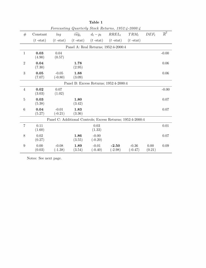
Table 1

Forecasting Quarterly Stock Returns, 1952:4-2000:4

# Constant lag cayt dt − pt RRELt TRMt DEFt R2

(t -stat) (t -stat) (t -stat) (t -stat) (t -stat) (t -stat)

Panel A: Real Returns; 1952:4-2000:4

1 0.03 0.04 -0.00(4.90) (0.57)

2 0.04 1.78 0.06(7.30) (2.95)

3 0.05 -0.05 1.88 0.06(7.07) (-0.80) (3.09)

Panel B: Excess Returns; 1952:4-2000:4

4 0.02 0.07 -0.00(3.03) (1.02)

5 0.03 1.80 0.07(5.38) (3.42)

6 0.04 -0.01 1.83 0.07(5.27) (-0.21) (3.36)

Panel C: Additional Controls; Excess Returns; 1952:4-2000:4

7 0.11 0.03 0.01(1.60) (1.33)

8 0.02 1.86 -0.00 0.07(0.27) (3.55) (-0.20)

9 0.00 -0.08 1.89 -0.01 -2.50 -0.36 0.00 0.09(0.03) (-1.38) (3.54) (-0.40) (-2.98) (-0.47) (0.21)

Notes: See next page.

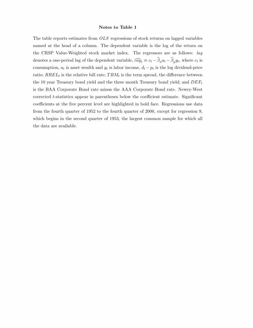
Notes to Table 1

The table reports estimates from OLS regressions of stock returns on lagged variables

named at the head of a column. The dependent variable is the log of the return on

the CRSP Value-Weighted stock market index. The regressors are as follows: lag

denotes a one-period lag of the dependent variable, cayt ≡ ct− βaat− βyyt, where ct is

consumption, at is asset wealth and yt is labor income, dt− pt is the log dividend-price

ratio; RRELt is the relative bill rate; TRMt is the term spread, the difference between

the 10 year Treasury bond yield and the three month Treasury bond yield; and DEFt

is the BAA Corporate Bond rate minus the AAA Corporate Bond rate. Newey-West

corrected t-statistics appear in parentheses below the coefficient estimate. Significant

coefficients at the five percent level are highlighted in bold face. Regressions use data

from the fourth quarter of 1952 to the fourth quarter of 2000, except for regression 9,

which begins in the second quarter of 1953, the largest common sample for which all

the data are available.

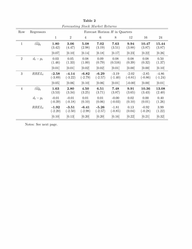
Table 2

Forecasting Stock Market Returns

Row Regressors Forecast Horizon H in Quarters

1 2 4 6 8 12 16 24

1 cayt 1.80 3.06 5.08 7.02 7.63 9.94 10.47 15.44(3.42) (4.47) (2.98) (3.19) (3.51) (3.88) (3.87) (3.87)

[0.07] [0.10] [0.14] [0.18] [0.17] [0.23] [0.22] [0.26]

2 dt − pt 0.03 0.05 0.08 0.09 0.08 0.08 0.08 0.50(1.46) (1.33) (1.00) (0.79) (0.516) (0.39) (0.32) (1.37)

[0.01] [0.01] [0.02] [0.02] [0.01] [0.00] [0.00] [0.10]

3 RRELt -2.58 -4.14 -6.82 -6.29 -3.19 -2.02 -2.85 -4.86(-3.89) (-3.22) (-2.79) (-2.57) (-1.40) (-0.81) (-0.86) (-1.24)

[0.05] [0.06] [0.10] [0.06] [0.01] [-0.00] [0.00] [0.01]

4 cayt 1.63 2.80 4.50 6.51 7.48 9.91 10.36 13.08(3.53) (3.34) (3.25) (3.71) (3.87) (3.65) (3.43) (2.40)

dt − pt -0.01 -0.01 0.01 0.01 -0.00 0.02 0.00 0.40(-0.39) (-0.18) (0.10) (0.06) (-0.03) (0.10) (0.01) (1.26)

RRELt -1.92 -3.51 -6.41 -5.26 -1.81 0.13 -0.92 3.99(-2.20) (-2.50) (-2.98) (-2.57) (-0.85) (0.04) (-0.28) (1.22)

[0.10] [0.13] [0.20] [0.20] [0.16] [0.22] [0.21] [0.32]

Notes: See next page.

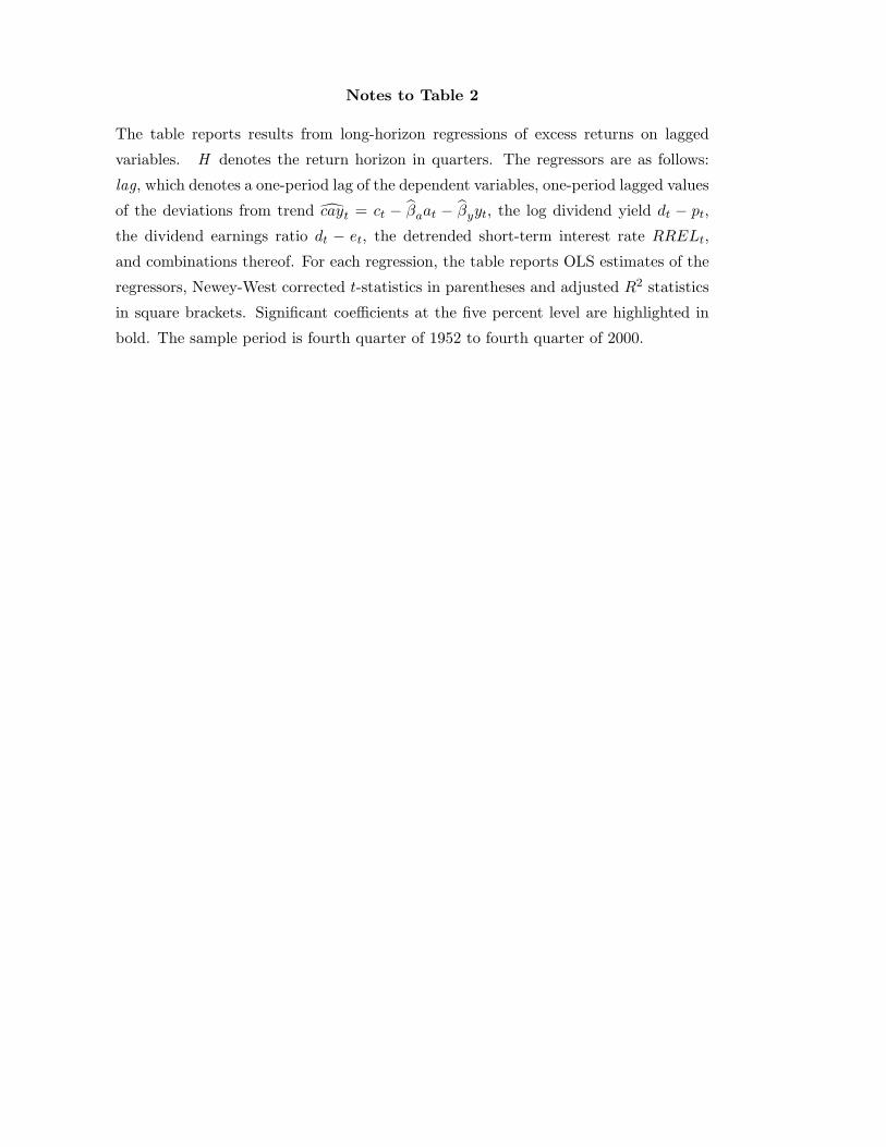
Notes to Table 2

The table reports results from long-horizon regressions of excess returns on lagged

variables. H denotes the return horizon in quarters. The regressors are as follows:

lag, which denotes a one-period lag of the dependent variables, one-period lagged values

of the deviations from trend cayt = ct − βaat − βyyt, the log dividend yield dt − pt,

the dividend earnings ratio dt − et, the detrended short-term interest rate RRELt,

and combinations thereof. For each regression, the table reports OLS estimates of the

regressors, Newey-West corrected t-statistics in parentheses and adjusted R2 statistics

in square brackets. Significant coefficients at the five percent level are highlighted in

bold. The sample period is fourth quarter of 1952 to fourth quarter of 2000.

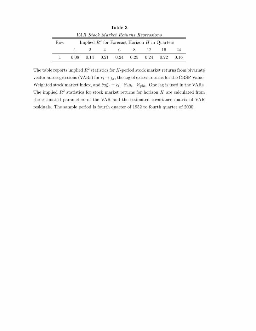
Table 3

VAR Stock Market Returns Regressions

Row Implied R2 for Forecast Horizon H in Quarters

1 2 4 6 8 12 16 24

1 0.08 0.14 0.21 0.24 0.25 0.24 0.22 0.16

The table reports implied R2 statistics forH-period stock market returns from bivariate

vector autoregressions (VARs) for rt−rf,t, the log of excess returns for the CRSP Value-

Weighted stock market index, and cayt ≡ ct−αaat−αyyt. One lag is used in the VARs.

The implied R2 statistics for stock market returns for horizon H are calculated from

the estimated parameters of the VAR and the estimated covariance matrix of VAR

residuals. The sample period is fourth quarter of 1952 to fourth quarter of 2000.

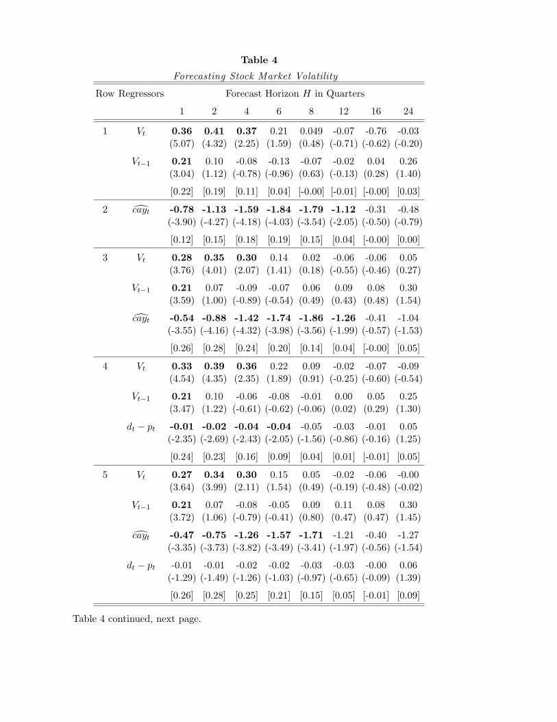
Table 4

Forecasting Stock Market Volatility

Row Regressors Forecast Horizon H in Quarters

1 2 4 6 8 12 16 24

1 Vt 0.36 0.41 0.37 0.21 0.049 -0.07 -0.76 -0.03(5.07) (4.32) (2.25) (1.59) (0.48) (-0.71) (-0.62) (-0.20)

Vt−1 0.21 0.10 -0.08 -0.13 -0.07 -0.02 0.04 0.26(3.04) (1.12) (-0.78) (-0.96) (0.63) (-0.13) (0.28) (1.40)

[0.22] [0.19] [0.11] [0.04] [-0.00] [-0.01] [-0.00] [0.03]

2 cayt -0.78 -1.13 -1.59 -1.84 -1.79 -1.12 -0.31 -0.48(-3.90) (-4.27) (-4.18) (-4.03) (-3.54) (-2.05) (-0.50) (-0.79)

[0.12] [0.15] [0.18] [0.19] [0.15] [0.04] [-0.00] [0.00]

3 Vt 0.28 0.35 0.30 0.14 0.02 -0.06 -0.06 0.05(3.76) (4.01) (2.07) (1.41) (0.18) (-0.55) (-0.46) (0.27)

Vt−1 0.21 0.07 -0.09 -0.07 0.06 0.09 0.08 0.30(3.59) (1.00) (-0.89) (-0.54) (0.49) (0.43) (0.48) (1.54)

cayt -0.54 -0.88 -1.42 -1.74 -1.86 -1.26 -0.41 -1.04(-3.55) (-4.16) (-4.32) (-3.98) (-3.56) (-1.99) (-0.57) (-1.53)

[0.26] [0.28] [0.24] [0.20] [0.14] [0.04] [-0.00] [0.05]

4 Vt 0.33 0.39 0.36 0.22 0.09 -0.02 -0.07 -0.09(4.54) (4.35) (2.35) (1.89) (0.91) (-0.25) (-0.60) (-0.54)

Vt−1 0.21 0.10 -0.06 -0.08 -0.01 0.00 0.05 0.25(3.47) (1.22) (-0.61) (-0.62) (-0.06) (0.02) (0.29) (1.30)

dt − pt -0.01 -0.02 -0.04 -0.04 -0.05 -0.03 -0.01 0.05(-2.35) (-2.69) (-2.43) (-2.05) (-1.56) (-0.86) (-0.16) (1.25)

[0.24] [0.23] [0.16] [0.09] [0.04] [0.01] [-0.01] [0.05]

5 Vt 0.27 0.34 0.30 0.15 0.05 -0.02 -0.06 -0.00(3.64) (3.99) (2.11) (1.54) (0.49) (-0.19) (-0.48) (-0.02)

Vt−1 0.21 0.07 -0.08 -0.05 0.09 0.11 0.08 0.30(3.72) (1.06) (-0.79) (-0.41) (0.80) (0.47) (0.47) (1.45)

cayt -0.47 -0.75 -1.26 -1.57 -1.71 -1.21 -0.40 -1.27(-3.35) (-3.73) (-3.82) (-3.49) (-3.41) (-1.97) (-0.56) (-1.54)

dt − pt -0.01 -0.01 -0.02 -0.02 -0.03 -0.03 -0.00 0.06(-1.29) (-1.49) (-1.26) (-1.03) (-0.97) (-0.65) (-0.09) (1.39)

[0.26] [0.28] [0.25] [0.21] [0.15] [0.05] [-0.01] [0.09]

Table 4 continued, next page.

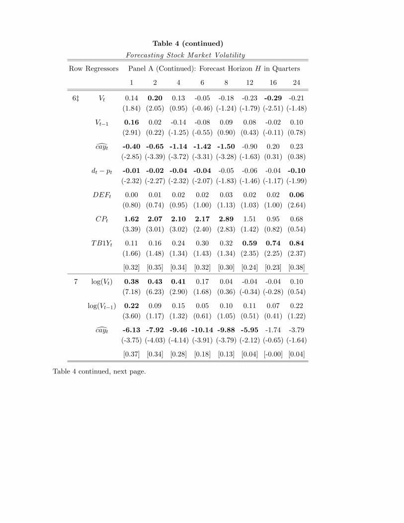
Table 4 (continued)

Forecasting Stock Market Volatility

Row Regressors Panel A (Continued): Forecast Horizon H in Quarters

1 2 4 6 8 12 16 24

6‡ Vt 0.14 0.20 0.13 -0.05 -0.18 -0.23 -0.29 -0.21

(1.84) (2.05) (0.95) (-0.46) (-1.24) (-1.79) (-2.51) (-1.48)

Vt−1 0.16 0.02 -0.14 -0.08 0.09 0.08 -0.02 0.10

(2.91) (0.22) (-1.25) (-0.55) (0.90) (0.43) (-0.11) (0.78)

cayt -0.40 -0.65 -1.14 -1.42 -1.50 -0.90 0.20 0.23

(-2.85) (-3.39) (-3.72) (-3.31) (-3.28) (-1.63) (0.31) (0.38)

dt − pt -0.01 -0.02 -0.04 -0.04 -0.05 -0.06 -0.04 -0.10

(-2.32) (-2.27) (-2.32) (-2.07) (-1.83) (-1.46) (-1.17) (-1.99)

DEFt 0.00 0.01 0.02 0.02 0.03 0.02 0.02 0.06

(0.80) (0.74) (0.95) (1.00) (1.13) (1.03) (1.00) (2.64)

CPt 1.62 2.07 2.10 2.17 2.89 1.51 0.95 0.68

(3.39) (3.01) (3.02) (2.40) (2.83) (1.42) (0.82) (0.54)

TB1Yt 0.11 0.16 0.24 0.30 0.32 0.59 0.74 0.84

(1.66) (1.48) (1.34) (1.43) (1.34) (2.35) (2.25) (2.37)

[0.32] [0.35] [0.34] [0.32] [0.30] [0.24] [0.23] [0.38]

7 log(Vt) 0.38 0.43 0.41 0.17 0.04 -0.04 -0.04 0.10

(7.18) (6.23) (2.90) (1.68) (0.36) (-0.34) (-0.28) (0.54)

log(Vt−1) 0.22 0.09 0.15 0.05 0.10 0.11 0.07 0.22

(3.60) (1.17) (1.32) (0.61) (1.05) (0.51) (0.41) (1.22)

cayt -6.13 -7.92 -9.46 -10.14 -9.88 -5.95 -1.74 -3.79

(-3.75) (-4.03) (-4.14) (-3.91) (-3.79) (-2.12) (-0.65) (-1.64)

[0.37] [0.34] [0.28] [0.18] [0.13] [0.04] [-0.00] [0.04]

Table 4 continued, next page.

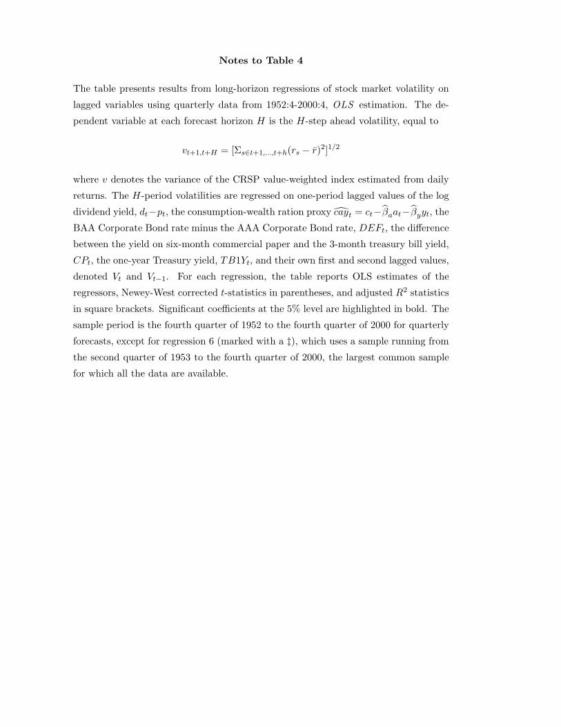
Notes to Table 4

The table presents results from long-horizon regressions of stock market volatility on

lagged variables using quarterly data from 1952:4-2000:4, OLS estimation. The de-

pendent variable at each forecast horizon H is the H-step ahead volatility, equal to

vt+1,t+H = [Σs∈t+1,...,t+h(rs − r)2]1/2

where v denotes the variance of the CRSP value-weighted index estimated from daily

returns. The H-period volatilities are regressed on one-period lagged values of the log

dividend yield, dt−pt, the consumption-wealth ration proxy cayt = ct−βaat−βyyt, the

BAA Corporate Bond rate minus the AAA Corporate Bond rate, DEFt, the difference

between the yield on six-month commercial paper and the 3-month treasury bill yield,

CPt, the one-year Treasury yield, TB1Yt, and their own first and second lagged values,

denoted Vt and Vt−1. For each regression, the table reports OLS estimates of the

regressors, Newey-West corrected t-statistics in parentheses, and adjusted R2 statistics

in square brackets. Significant coefficients at the 5% level are highlighted in bold. The

sample period is the fourth quarter of 1952 to the fourth quarter of 2000 for quarterly

forecasts, except for regression 6 (marked with a ‡), which uses a sample running from

the second quarter of 1953 to the fourth quarter of 2000, the largest common sample

for which all the data are available.

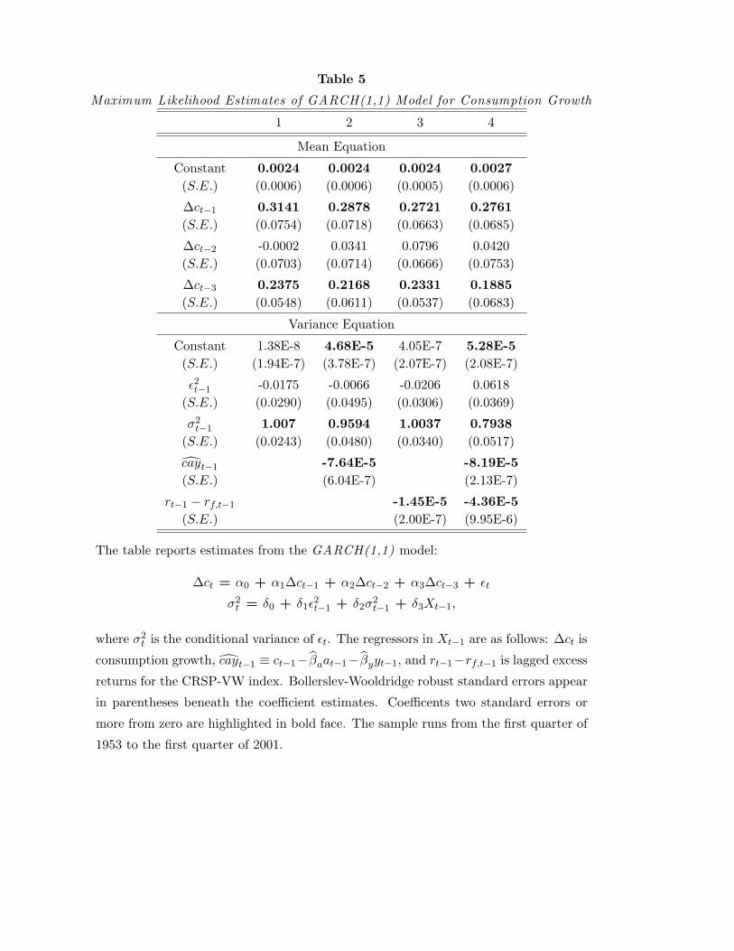
Table 5

Maximum Likelihood Estimates of GARCH(1,1) Model for Consumption Growth

1 2 3 4

Mean Equation

Constant 0.0024 0.0024 0.0024 0.0027

(S.E.) (0.0006) (0.0006) (0.0005) (0.0006)

∆ct−1 0.3141 0.2878 0.2721 0.2761

(S.E.) (0.0754) (0.0718) (0.0663) (0.0685)

∆ct−2 -0.0002 0.0341 0.0796 0.0420

(S.E.) (0.0703) (0.0714) (0.0666) (0.0753)

∆ct−3 0.2375 0.2168 0.2331 0.1885

(S.E.) (0.0548) (0.0611) (0.0537) (0.0683)

Variance Equation

Constant 1.38E-8 4.68E-5 4.05E-7 5.28E-5

(S.E.) (1.94E-7) (3.78E-7) (2.07E-7) (2.08E-7)

ε2t−1 -0.0175 -0.0066 -0.0206 0.0618

(S.E.) (0.0290) (0.0495) (0.0306) (0.0369)

σ2t−1 1.007 0.9594 1.0037 0.7938

(S.E.) (0.0243) (0.0480) (0.0340) (0.0517)

cayt−1 -7.64E-5 -8.19E-5

(S.E.) (6.04E-7) (2.13E-7)

rt−1 − rf,t−1 -1.45E-5 -4.36E-5

(S.E.) (2.00E-7) (9.95E-6)

The table reports estimates from the GARCH(1,1) model:

∆ct = α0 + α1∆ct−1 + α2∆ct−2 + α3∆ct−3 + εt

σ2t = δ0 + δ1ε

2t−1 + δ2σ

2t−1 + δ3Xt−1,

where σ2t is the conditional variance of εt. The regressors in Xt−1 are as follows: ∆ct is

consumption growth, cayt−1 ≡ ct−1−βaat−1−βyyt−1, and rt−1−rf,t−1 is lagged excess

returns for the CRSP-VW index. Bollerslev-Wooldridge robust standard errors appear

in parentheses beneath the coefficient estimates. Coefficents two standard errors or

more from zero are highlighted in bold face. The sample runs from the first quarter of

1953 to the first quarter of 2001.

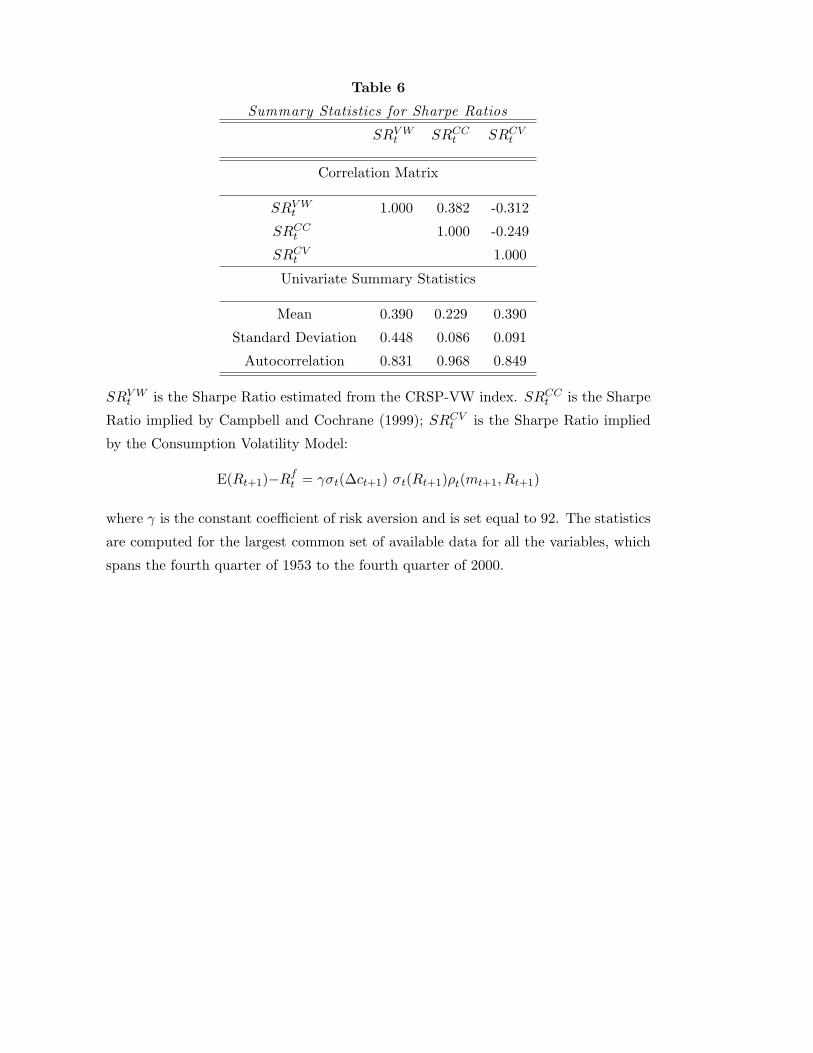
Table 6

Summary Statistics for Sharpe Ratios

SRVWt SRCC

t SRCVt

Correlation Matrix

SRVWt 1.000 0.382 -0.312

SRCCt 1.000 -0.249

SRCVt 1.000

Univariate Summary Statistics

Mean 0.390 0.229 0.390

Standard Deviation 0.448 0.086 0.091

Autocorrelation 0.831 0.968 0.849

SRVWt is the Sharpe Ratio estimated from the CRSP-VW index. SRCC

t is the Sharpe

Ratio implied by Campbell and Cochrane (1999); SRCVt is the Sharpe Ratio implied

by the Consumption Volatility Model:

E(Rt+1)−Rft = γσt(∆ct+1) σt(Rt+1)ρt(mt+1, Rt+1)

where γ is the constant coefficient of risk aversion and is set equal to 92. The statistics

are computed for the largest common set of available data for all the variables, which

spans the fourth quarter of 1953 to the fourth quarter of 2000.

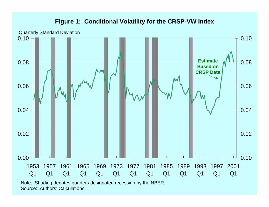
0.00

0.02

0.04

0.06

0.08

0.10

1953Q1

1957Q1

1961Q1

1965Q1

1969Q1

1973Q1

1977Q1

1981Q1

1985Q1

1989Q1

1993Q1

1997Q1

2001Q1

0.00

0.02

0.04

0.06

0.08

0.10

Figure 1: Conditional Volatility for the CRSP-VW Index

Quarterly Standard Deviation

Note: Shading denotes quarters designated recession by the NBERSource: Authors’ Calculations

EstimateBased on

CRSP Data

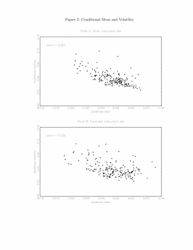
Figure 2: Conditional Mean and Volatility

Note: This figure illustrates the relation between the conditional mean and conditional volatility of excessreturns on the CRSP value weighted stock index. The conditioning information in Panel A is based on asmall instrument set in which cayt is the sole instrument for returns, and cayt and two lags of volatility areinstruments for volatility. The conditioning information in Panel B is based on an expanded instrument set inwhich cayt, dt − pt and RRELt are instruments for returns, and cayt, two lags of volatility, dt − pt, DEFt, CPtand TB1Yt are instruments for volatility. The sample is quarterly and spans the period 1953:Q4 to 2000:Q4.

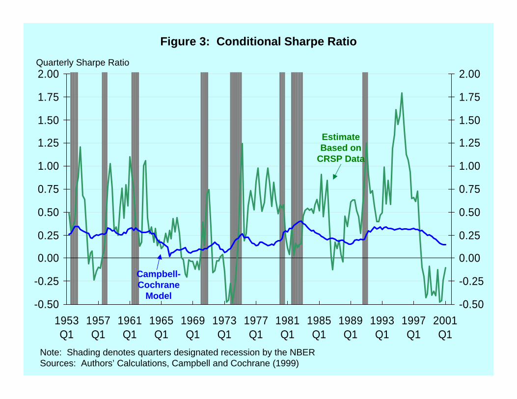
-0.50

-0.25

0.00

0.25

0.50

0.75

1.00

1.25

1.50

1.75

2.00

1953Q1

1957Q1

1961Q1

1965Q1

1969Q1

1973Q1

1977Q1

1981Q1

1985Q1

1989Q1

1993Q1

1997Q1

2001Q1

-0.50

-0.25

0.00

0.25

0.50

0.75

1.00

1.25

1.50

1.75

2.00

Figure 3: Conditional Sharpe Ratio

Quarterly Sharpe Ratio

Note: Shading denotes quarters designated recession by the NBERSources: Authors’ Calculations, Campbell and Cochrane (1999)

EstimateBased on

CRSP Data

Campbell-Cochrane

Model

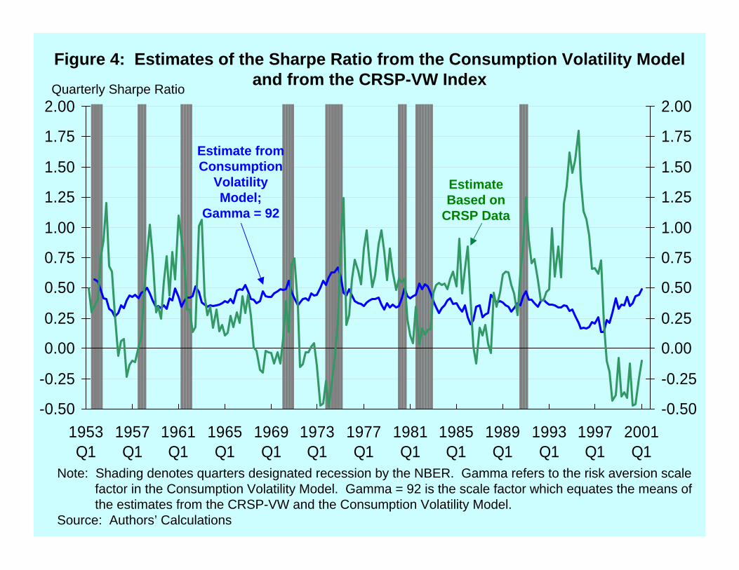
-0.50

-0.25

0.00

0.25

0.50

0.75

1.00

1.25

1.50

1.75

2.00

1953Q1

1957Q1

1961Q1

1965Q1

1969Q1

1973Q1

1977Q1

1981Q1

1985Q1

1989Q1

1993Q1

1997Q1

2001Q1

-0.50

-0.25

0.00

0.25

0.50

0.75

1.00

1.25

1.50

1.75

2.00

Figure 4: Estimates of the Sharpe Ratio from the Consumption Volatility Modeland from the CRSP-VW Index

Quarterly Sharpe Ratio

Note: Shading denotes quarters designated recession by the NBER. Gamma refers to the risk aversion scalefactor in the Consumption Volatility Model. Gamma = 92 is the scale factor which equates the means ofthe estimates from the CRSP-VW and the Consumption Volatility Model.

Source: Authors’ Calculations

EstimateBased on

CRSP Data

Estimate fromConsumption

VolatilityModel;

Gamma = 92