Embed Size (px)
Citation preview

1
Measuring Individual Economic Well-Being and Social Welfare within the
Framework of the System of National Accounts
Keywords: Welfare measurement, national accounts, distribution of consumption
JEL: E210, D31, D63
Abstract
While the agenda of “beyond GDP” encompasses measurements that lie outside boundaries of the System of National Accounts, key aspects of individual well-being and social welfare can be incorporated into an SNA framework. We bring together the relevant theoretical literature and the empirical tools needed for this purpose. We show how consumption-based measures of economic welfare can be integrated into the national accounts without changing their production or asset boundary. At the same time, explicit normative and methodological choices are required to select a social welfare function. The paper provides guidance how to make these choices transparent and how to present social welfare measures.

2
1. Introduction
Renewed interest in the measurement of individual well-being and social welfare is evident in
the recommendations by Stiglitz, Sen, and Fitoussi (2010) on the measurement of economic
performance and social progress and the G20 Data Gaps Initiative (2009) on enhancements in
economic and financial statistics. While the agenda of “beyond GDP” encompasses measurements
that lie outside the production and asset boundaries of The System of National Accounts 2008
(2009), key aspects of individual well-being and social welfare can be incorporated into the
framework of the SNA 2008. A leading example is the measures of individual and social welfare
proposed by Jorgenson and Slesnick (2014).
The common features of the Stiglitz-Sen-Fitoussi and Data Gaps reports are a focus on income,
consumption and wealth, rather than production, and an emphasis on disparities among members
of the population rather than national aggregates. In response to the interest in income,
consumption/saving, and wealth, the OECD and Eurostat established an Expert Group on
Disparities in a National Accounts framework (EG DNA) to consider standards for the measurement
of disparities within the framework of the national accounts. A second OECD-Eurostat Expert
Group on Income, Consumption and Wealth (EG ICW) considered consistency between definitions
of these concepts in macro-economic data from the national accounts and micro-economic data
from household surveys and administrative records.
Initial results have been reported by Fesseau, Wolff, and Mattonetti (2013) and Fesseau and
Mattonetti (2013).

3
The expert group on disparities has collected information from leading statistical agencies on
the role of distributional information in the national accounts and existing capabilities for providing
the necessary survey information. The expert group has discussed the reconciliation of national
accounting aggregates with survey statistics and have given detailed empirical examples of methods
for incorporation of these statistics into the 2008 SNA. Our work embeds these statistical advances
in a broader theoretical framework based on Jorgenson and Slesnick (2014) and proposes measures
of individual economic well-being as well as summary measures of social welfare.
The measurement of individual economic well-being is based on a long-established theory of
consumer behaviour.1 This is useful in choosing among the many possible approaches to the
measurement of consumption considered in the literature and could be helpful in extending these
approaches beyond the boundaries of the 2008 SNA, which we do not consider in this paper. The
first issue is the definition of the consumption unit. In economic surveys consumption is measured
for households, consisting of individuals living together and sharing a budget. While the theory of
consumer behaviour deals with the individuals, rather than households, there is also a well-
established, if less familiar, theory of household behaviour that can serve as a valuable guide to the
measurement of consumption.
We thus take the household, rather than the individual, as the starting point for the measurement
of consumption at the micro-economic level. This results in a second issue for economic statistics,
namely, that a large household requires more measured consumption than a small household to
achieve the same level of well-being. However, such differences are not necessarily proportional to
household size. In measuring disparities among consuming units economic statisticians have
1The year 2015 is the centennial of Eugen (Evgeny) Slutsky (1915), “Sulla theoria del bilancio del consumatore,”
Giornale degli Economisti, 51(3): 1-26, often taken as the starting point for the theory of consumer behaviour.
4
introduced household equivalence scales to capture differences in the composition of households.
At a minimum these scales depend on the number of individuals, but Jorgenson and Slesnick (1987)
have shown how to use an econometric model of household behaviour to derive equivalence scales
that depend on other characteristics of household composition as well. We compare the effect of
using a uni-dimensional, size-related household scale with the Jorgenson-Slesnick multi-
dimensional household scale and find important differences with likely effects on measured living
standards.
In this paper we consider the measurement of individual welfare in Section 2. By way of
example, we use information from the U.S. consumer expenditure survey and control totals from
the national accounts to construct measures of individual well-being. These measures incorporate
differences in prices and total expenditure along with information about household composition.
The distribution of individual welfare over a given population provides the information required to
quantify differences among households. These are the “disparities” of EG DNA and can be
integrated into the national accounts along with accounting aggregates like consumer expenditures.
It is useful to emphasize that consumer expenditures could be augmented in various ways, recently
summarized by Abraham (2014), but this would involve changing the boundaries of the national
accounts.
The measurement of social welfare is based on the economic theory of social choice. This
provides a framework useful in choosing among the many approaches for measuring social welfare
considered in the literature. Measures of social welfare are based on the distribution of consumption
scaled by a measure of household size. We refer to this as the distribution of household equivalent

5
consumption.2 While measures of individual welfare depend on optimization by households, no
optimization is involved in deriving measures of social welfare from the theory of social choice.
However, by contrast with measures of individual welfare, social welfare measures depend on
normative assumptions or value judgements. Jorgenson and Slesnick (2014) have shown how to
incorporate these normative assumptions into measures of social welfare within the framework of
the national accounts. We discuss some of the properties of the Jorgenson-Slesnick social welfare
measure and compare them with the welfare measure proposed by Atkinson (1970).
We also refer to a measure of social welfare as the standard of living. We consider only those
measures of the standard of living that are feasible, given information about individual welfare
available within the framework of the national accounts. Following Atkinson (1970), we decompose
measures of social welfare between measures of efficiency and equity. Measures of equity can be
transformed into measures of inequity or inequality. Our measures of efficiency can be expressed
in terms of national accounting aggregates in particular real personal consumption expenditure per
household equivalent member.
In Section 4 we conclude that economic statisticians should use measures of social welfare,
including efficiency and equity, to summarize information about the distribution of individual
welfare. We emphasize that this can be done within the 2008 SNA. Fortunately, the practical issues
that confront statistical agencies in measuring individual well-being and social welfare have been
discussed exhaustively by EG ICW and EG DNA.
2 The term “equivalised consumption” is sometimes used for scaled household consumption, but “household
equivalent consumption” conveys the same meaning and is closer to standard English usage.
6
2. Measures of individual economic well-being
Whose well-being? Households, individuals and equivalence scales
Our investigation starts at the micro-economic level with a question about the nature of the
consuming unit. The key lies in the distinction between households and individuals. Although the
traditional theory of consumer behaviour is based on individuals, more in-depth analysis has
recognised that the household is a more appealing way to think about decision-making units. The
necessary framework was provided by the theory of household behaviour of Samuelson (1956).3
Our starting point for welfare comparisons is thus the household. This coincides with the fact that
empirical sources of information on consumption or income are typically collected for households,
not individuals. At the same time, households may have quite different characteristics, for example
in terms of the number of individuals living in a household so it is not obvious whether one
household’s economic well-being can be directly compared to another household’s well-being
unless they share the same characteristics.
The single most frequently used characteristic is household size. The Canberra Group
Handbook on Household Income Statistics describes this as follows: “ […] the needs of a household
grow with each additional member but, due to economies of scale in consumption, not in a
proportional way. For example, a household comprising three people would normally need more
income than a lone person household if the two households are to enjoy the same standard of living.
However, a household with three members is unlikely to need three times the housing space,
electricity, etc. that a lone person household requires.” (UN-ECE 2011, p. 68)
3 Samuelson’s theory has been discussed by Becker (1981) and Pollak (1981).

7
“Equivalised consumption or income is an indicator for welfare comparisons across
standardised households or for a household comprising more than one person, equivalised income
is an indicator of the household income that would be needed by a lone person household to enjoy
the same level of economic welfare as the household in question.” (UN-ECE 2011, p. 68)
An example of such a simplified approach is the OECD modified equivalence scale (Hagenaars
et al. 1994), commonly used in statistical work. Within each household, the first adult counts 1, all
children under 14 get a weight of 0.3 and any additional person aged 14 and above gets a weight of
0.5. The original ‘OECD equivalence scale’ (OECD 1982, also called “Oxford scale”) assigned a
value of 1 to the first household member, of 0.7 to each additional adult and of 0.5 to each child.
Recent OECD publications (e.g. OECD 2011, OECD 2008) comparing income inequality and
poverty across countries have used a scale which divides household income by the square root of
household size.
The economic theory of equivalence scales (see Lewbel and Pendakur 2008 for an overview)
takes a more general starting point and defines equivalence scales as the proportional change in
expenditure that is required to equalise utility between two households with different characteristics.
In this vein, Barten (1964) proposed an approach where equivalence scales varied across types of
commodities. As these equivalence scales depend on expenditure patterns, they vary not only with
household size but also with prices and household characteristics that shape expenditure patterns.
As a consequence, equivalence scales become multi-dimensional. Muellbauer (1977) estimated
Barten scales for the United Kingdom, Johnson (1994) and Slesnick and Jorgenson and Slesnick
(1987, 2014) estimated Barten scales for the United States. Table 1 reproduces Barten scales
estimated by Jorgenson and Slesnick (1987).
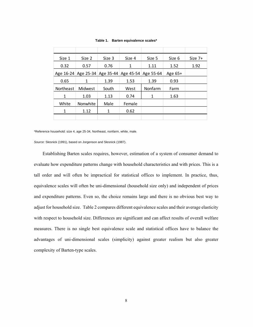
8
Table 1. Barten equivalence scales*
*Reference household: size 4, age 25-34, Northeast, nonfarm, white, male.
Source: Slesnick (1991), based on Jorgenson and Slesnick (1987).
Establishing Barten scales requires, however, estimation of a system of consumer demand to
evaluate how expenditure patterns change with household characteristics and with prices. This is a
tall order and will often be impractical for statistical offices to implement. In practice, thus,
equivalence scales will often be uni-dimensional (household size only) and independent of prices
and expenditure patterns. Even so, the choice remains large and there is no obvious best way to
adjust for household size. Table 2 compares different equivalence scales and their average elasticity
with respect to household size. Differences are significant and can affect results of overall welfare
measures. There is no single best equivalence scale and statistical offices have to balance the
advantages of uni-dimensional scales (simplicity) against greater realism but also greater
complexity of Barten-type scales.
Size 1 Size 2 Size 3 Size 4 Size 5 Size 6 Size 7+
0.32 0.57 0.76 1 1.11 1.52 1.92
Age 16‐24 Age 25‐34 Age 35‐44 Age 45‐54 Age 55‐64 Age 65+
0.65 1 1.39 1.53 1.39 0.93
Northeast Midwest South West Nonfarm Farm
1 1.03 1.13 0.74 1 1.63
White Nonwhite Male Female
1 1.12 1 0.62

9
Table 2. Different equivalence scales
Another, related measurement issue is the level of detail at which distributional measures are
put in place. Ideally, the equivalence scales are directly applied to household-level information. In
practice, another simplifying assumption is often used in empirical measurements. Rather than
applying equivalence scales (and, as will be discussed below, price indices) at the level of individual
households, groups of households are the object of measurement in the simplified case. Each group
is treated like a single, homogenous household. A natural way of grouping individual households
is forming quintiles or deciles based on households’ consumption or income. For instance, results
of the U.S. consumer expenditure survey are published by quintiles defined over primary income
of households. Jorgenson and Slesnick (1987, 2014) allow for a much more granular treatment of
households – grouping and the scaling of consumer expenditure take place for individual
households with identical demographic characteristics.
Whose price index? Recognising differences in expenditure structures
Much of the literature on the distribution of income or consumption has focused on how these
attributes are distributed among agents at a point in time but has paid less attention on how to render
group-specific income or consumption comparable both between households and over time. The
Household
size
Per
capita
measure
Barten
scale (size
dimension
only)
OECD
(old)
OECD
(square
root
formula)
1 1.00 1.00 1.00 1.00
2 1.00 0.83 0.77 0.50
3 1.00 0.79 0.72 0.50
4 1.00 0.82 0.72 0.50
5 1.00 0.77 0.72 0.50
6 1.00 0.87 0.73 0.50
7 1.00 0.92 0.74 0.50

10
conceptually correct measure of price changes is a cost-of-living index (Konüs 1929). As
households with different levels of consumption or income will feature different expenditure
patterns, their cost-of-living indexes will in general be different and consequently, deflation of
nominal consumption or income should proceed by means of a group-specific price index.
Separate cost of living indices for groups of households can be constructed as long as there is
information on expenditure patterns for each type of household. If no such possibility exists, a rather
strong assumption has to be invoked, namely that preferences of a household only depend on
relative prices but are otherwise independent of the level of household welfare4 which may only
affect the level of expenditures in a proportional way. The advantage of this simplification is that a
single price index can be applied to deflate consumption or income for all households.
However, this trade-off appears to be of limited effects when examined empirically. Slesnick
(2001) computes cost-of-living indices for household groups with different consumption levels for
the time period 1948- 1995 and concludes that “…the inflation rates for the three groups are […]
very similar” (p. 84). In our own empirical example based on recent data from the U.S. Consumer
Expenditure Survey we construct a set of expenditure weights for each product group, household
group and year under consideration. Weights from adjacent years are combined with the price
changes for each product group to construct a Fisher price index of final household consumption
expenditure by household income quintile. For the period 2005-2013 differences between price
indices for the five groups of households are small, ranging between 1.9% and 2.1% per year. The
4 Independence from welfare levels implies homotheticity - a necessary and sufficient condition for the independence
of the price index from the level utility, as shown by Malmquist (1953).

11
use of an aggregate price index for different consumption groups would thus not appear to be a
specifically constraining assumption5.
Even if a single price index is chosen for different households, there are several choices, for
example the private consumption deflator from the national accounts, and various variants of the
Consumer Price Index (CPI). Meyer and Sullivan (2011) and Broda and Weinstein (2009) show the
important impact of alternative price indices. Fixler and Johnson (2014) opt for the Personal
Consumption Expenditures (PCE) deflator on the grounds that their work focuses on a national
accounts-based measure of income and its distribution. The same reasoning applies to the
calculations at hand where consumption expenditure for the various product groups will be deflated
with price indices from the national accounts. We conclude that applying the deflator for private
consumption expenditure from the national accounts constitutes a reasonable method to derive
measures of real consumption.
A measure of households’ economic well-being
Having dealt with equivalence scales, deflation and the scope of consumption, we can now
explicitly state a measure Wk of individual welfare for household k (k=1,…K):
W W V withV ∙ (1)
In (1), p is a vector of N prices of consumer products and xk is a vector of N quantities of products
consumed by household k. Real consumption per household equivalent member Vk is derived by
5 Note that this conclusion is based on a single characteristic, income, to group households and measure their cost-of-
living index. Differentiation by other characteristics, in particular age, has been shown to yield more diverse results (Slesnick 2001). Thus, with more complete information, for instance from econometric measurement that permits identifying expenditure patterns across multiple dimensions one may well find more pronounced differences between price indices for different groups of households.

12
deflating the nominal value of expenditure p·xk≡∑ipixi,k by a household-specific price index Gk(p)
or, in a simplified approach, by a general price index G(p). Real consumption per household is then
transformed into consumption per household equivalent member by applying an equivalence scale
m0(Ak) corresponding to household k’s characteristics Ak. As discussed earlier, in the simplest case
this is a function of household size only but in general captures multiple household characteristics.
The scope and valuation of the products entering a household’s utility function are captured by
private consumption expenditure here. The implication is that those goods and services that are
provided for free by the government will not be captured by this expenditure measure despite the
fact that they generate utility for the household. Or they will be valued at a price below cost in the
case of subsidisation. An alternative would thus be to select a measure of Actual Individual
Consumption that includes Social Transfers in Kind, such as free health care, education or housing.
However, prices and volumes of a measure of actual individual consumption do not reflect the
consumer decisions in the face of a set of prices. Also, data availability is significantly more limited.
The expenditure framework used is best understood as cost-minimising behaviour on the side of
consumers, conditional on a set of publicly-provided services.
Jorgenson and Slesnick (1984, 2014) set Wk as the logarithmic transformation measure of the real
expenditure measure Vk, (Wk=ln(Vk)) implying that utility gains are decreasing with increasing
consumption. In a more complete setting such as Jorgenson and Slesnick (1984, 2014) the
individual measure of welfare is derived as a household’s minimum expenditure to achieve a
particular level of utility, Wk, given prices p. Vk(Wk, Ak, p) then equals the household’s expenditure
function which provides an exact representation of the underlying level of the household’s utility 6.
6 In the present framework, utility only depends on the level of consumption and household characteristics. Outside the
framework of the national accounts, household utility could also depend on factors such as the health of

13
Which consumption? Which income? From surveys to the national accounts
An underlying premise to this point has been that consumer expenditure or income, and prices
and quantities of consumer products are readily observable for each household or group of
households. This is not a matter of course when national accounts definitions of consumption and
income are used as the benchmark or target definitions (Deaton 2005). Yet, taking national accounts
benchmarks is a necessary step to derive national accounts-consistent welfare comparisons that can
be compared with other national accounts variables such as GDP per capita. The national accounts
framework is particularly useful as it provides a consistent link between primary and disposable
income, consumption, savings and wealth.
In many instances national accounts estimates may be expected to be of higher quality than
those from micro-sources due to the focus of national accounts on consistent and exhaustive
estimates (Fesseau and Mattonetti 2013). The big disadvantage of national accounts data in the
present context is that distributional information – essential for measures of economic well-being –
is missing. Statistical groundwork is therefore required to use the informational contents from
survey information about distributions of consumption or income across households and apply it to
national accounts benchmarks. This cannot be done in an indiscriminate manner and requires
careful comparison of definitions and contents of income and consumption categories in surveys
and in national accounts.
Fixler and Johnson (2014) report on early estimates by Budd and Radner (1975) who combine
survey and tax data sources to construct a distributional measure for the national accounts. Fesseau,
household members, environmental quality or social relations. While the latter factors are clearly important, we leave these non-market variables aside here and focus on economic well-being. For an extension to non-market variables see Fleurbaey and Blanchet (2013).

14
Bellamy and Raynaud (2009) use survey data combined with other statistical sources to develop a
national accounts compatible distribution statistic for France. This work was brought to the
international level by the OECD and Eurostat in 2013. In cooperation with 25 national statistical
offices, survey-based information on the level and distribution of consumption and income
categories were matched to the national accounts, following a common methodology. The various
steps involved along with results for a recent year are described in Fesseau and Mattonetti (2013).
As the authors note, the introduction of national accounts concepts is not innocuous: inequality
measures such as the ratio of income or consumption of the richest over the poorest quintile of
households tend to be adjusted downwards when compared to survey-based measures. At the same
time, this effect depends on the specific choice of income or consumption variables. One such
choice is between final consumption expenditure and actual individual consumption: the latter
includes social transfers in kind, i.e., health, education and housing services provided for free or at
a below-market price by the government. As these services tend to be disproportionally used by
low-income households, inequality measures based on actual individual consumption tend to turn
out lower than inequality measures based on final consumption expenditure7.
Similarly, Fixler and Johnson (2014) present a methodology that adjusts the U.S. Current
Population Survey – a household survey – to more closely match the national accounts measure of
personal income. The authors then complement the survey source with data from tax returns to
obtain more granular information on income distribution and apply this to the national accounts
7 A similar reasoning applies to income-based measures of inequality: those based on adjusted disposable income
(which reflects social transfers in kind) tend to produce lower levels of inequality than those based on
disposable income or those based on primary income.
15
benchmarks of disposable household income. Like Fesseau and Mattonetti (2013), a further step by
the authors consists in imputing values for social transfers in kind.
Our simplified example uses results from the U.S. Consumer Expenditure Survey as conducted
and published by the U.S. Bureau of Labor Statistics. We match 15 expenditure categories to the
expenditure categories available in the OECD’s Annual National Accounts database8 (Table 3).
Clearly, this is a much rougher approximation than the match by Fesseau and Mattonetti (2013) or
Fixler and Johnson (2014) but it serves the purpose of demonstrating feasibility of proceeding in
this direction. The advantage of our approach is that it can readily be applied to several years and
we shall present results for the period 2005-2013.
Table 3 shows only the mapping between expenditure categories and adjustment coefficients
for 2013 but the figures are representative for other years as well. For the majority of categories,
the national accounts figure exceeds the figure from the Consumer Expenditure Survey. An
important step in national accounts-based computations of individual and social welfare consists
thus of matching consumer expenditure data for each product category and quintile of households
between survey and national accounts sources. For consumption categories that are not present in
8 The consumer expenditure survey provides expenditures for each category cross-classified by household income
group. Thus, for every income group, the survey-based expenditure measure is multiplied by the adjustment
factor to arrive at the relevant variable Vk for household (income group) k. If there is added information
about the distribution across income groups of those national accounts expenditure positions that are outside
the survey measure, this information can of course be used and adjustment factors would vary across income
groups. The consumer expenditure survey also provides information of the average household size for each
income group. To this information is applied an equivalence scale so to obtain the average number of
household equivalent members per income quintile. Averaging across income groups (as these are quintiles
with equal numbers of households each a simple average suffices) and multiplying by the economy-wide
number of households yields the total household equivalent members.
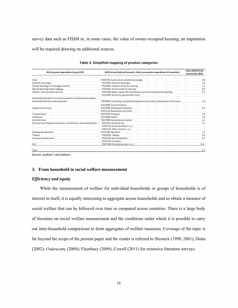
16
survey data such as FISIM or, in some cases, the value of owner-occupied housing, an imputation
will be required drawing on additional sources.
Table 3. Simplified mapping of product categories
Source: authors’ calculations.
3. From household to social welfare measurement
Efficiency and equity
While the measurement of welfare for individual households or groups of households is of
interest in itself, it is equally interesting to aggregate across households and so obtain a measure of
social welfare that can be followed over time or compared across countries. There is a large body
of literature on social welfare measurement and the conditions under which it is possible to carry
out inter-household comparisons to form aggregates of welfare measures. Coverage of the topic is
far beyond the scope of the present paper and the reader is referred to Slesnick (1998, 2001), Dutta
(2002); Chakravarty (2009); Fleurbaey (2009), Cowell (2011) for extensive literature surveys.
Ratio ANA/CES (all
households, 2013)
Food P31CP010: Food and non‐alcoholic beverages 0.9
Alcoholic beverages P31CP021: Alcoholic beverages 2.2
Owned dwellings incl mortgage interest P31CP042: Imputed rentals for housing 1.7
Rented dwellings+other lodgings P31CP041: Actual rentals for housing 0.9
Utilities, fuel and public services P31CP044: Water supply and miscellaneous services relating to the dwelling 0.7
P31CP045: Electricity, gas and other fuels
P31CP050: Furnishings, households equipment and routine maintenance of the house 1.8
P31CP080: Communications
Apparel and services P31CP030: Clothing and footwear 5.4
P31CP110: Restaurants and hotels
Transportation P31CP070: Transport 1.0
Healthcare P31CP060: Health 5.2
Entertainment P31CP090: Recreation and culture 3.3
Personal care products and services, miscallenous, cash contributions P31CP121: Personal care 1.3
P31CP123: Personal effects n. e. c.
P31CP127: Other services n. e. c.
Reading and education P31CP100: Education 1.7
Tobacco P31CP022: Tobacco 2.6
Insurance and pensions P31CP124: Social protection 0.7
P31CP125: Insurance
N.A. P31CP126: Financial services n. e. c. N.A.
Total 1.7
Household operations (incl communication), housekeeping supplies,
household furnishces and equipment
BLS Consumer Expenditure Survey (CES) OECD Annual National Accounts, finale consumption expenditure of households

17
We limit our considerations to issues that are important in the implementation of social welfare
functions. A key ingredient to construct measures of social welfare is the measures of individual
welfare, based on real consumption V W , A , p ∙ as presented above. Consider the
following average measure V obtained by dividing aggregate expenditure by the total number of
household equivalent members and by applying a consumption price index:
V∑ ∙
∑∑
∑
∙ ∑ s V ,
where:
s ≡∑
. (2)
We can interpret V “…as an indicator of efficiency since it is independent of the distribution
of welfare across households. That is, a transfer of resources from a rich household to a poor
household leaves V unchanged” (Slesnick 2001, p. 27). Efficiency is a distribution-free measure of
social welfare, attained at current prices p for a given aggregate expenditure and population of
household equivalent members. This measure is directly available from the national accounts, after
adjusting real expenditure for the total number of household equivalent persons.
Efficiency V is instrumental in de-composing a measure of social welfare that does take
account of distributional considerations into efficiency and equity components. To this end, define
a social welfare function as:
W = W(W1, W2,…WK), (3)

18
where Wk=Wk(Vk) (k=1,…K) is individual well-being. Some key properties of social welfare
functions along with two alternative specifications are given in the Annex. Here it suffices to recall
that individual welfare has been measured as a function of real consumption expenditure. Similarly,
we can define a welfare measure at the level of the total economy, call it V*(W)9:
W(V*, …V*) = W( W1(V1), W2(V2),…WK(VK) ), (4)
where V*=V*(W) is implicitly defined as the income (or consumption) that, if received by every
individual, yields the same social welfare as the actual distribution10. We also refer to this measure
of social welfare as the standard of living.
Given V*(W), and V, we can apply Jorgenson’s (1990) de-composition of V*(W) into equity
and efficiency components:
V∗ W ∗
V. (5)
The efficiency component V was defined above. The other component of (5), V*(W)/V,
compares actual social welfare V*(W) with potential maximum11 social welfare V and thus captures
the relative loss in social welfare attributable to an inequitable distribution. This is the ‘equity’
component of Jorgenson’s decomposition. Its derivation requires information about the distribution
of consumption per household equivalent member among individuals (or groups of households)
9 Kolm (1969) used the label equal equivalent, Atkinson (1970) equally distributed equivalent income.
10 This is a simplified version of Jorgenson and Slesnick’s (1984, 2014) social expenditure function.
11 Note that the efficiency measure V can also be interpreted as the level of equally distributed consumption that would give rise to maximum social welfare: one property often assumed for the welfare function W is that it reflects the Dalton (1920) principle which states that a transfer from someone with higher consumption to someone with less is welfare-increasing, as long as the transfer does not lead to a change in ranks between individuals concerns and as long as the transfer is non-leaky (nothing gets lost in the course of re-distribution). If W is reflective of the Dalton principle (along with several other properties), W reaches its maximum under equal distribution of income. See Diewert (1985, Theorem 2) for a formal statement.
19
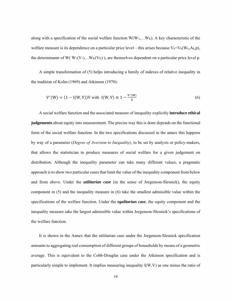
along with a specification of the social welfare function W(W1,…WK). A key characteristic of the
welfare measure is its dependence on a particular price level – this arises because Vk=Vk(Wk,Ak,p),
the determinants of W( W1(V1)…WK(VK) ), are themselves dependent on a particular price level p.
A simple transformation of (5) helps introducing a family of indexes of relative inequality in
the tradition of Kolm (1969) and Atkinson (1970):
V∗ W 1 I W, V V with I W, V ≡ 1∗
(6)
A social welfare function and the associated measure of inequality explicitly introduce ethical
judgements about equity into measurement. The precise way this is done depends on the functional
form of the social welfare function. In the two specifications discussed in the annex this happens
by way of a parameter (Degree of Aversion to Inequality), to be set by analysts or policy-makers,
that allows the statistician to produce measures of social welfare for a given judgement on
distribution. Although the inequality parameter can take many different values, a pragmatic
approach is to show two particular cases that limit the value of the inequality component from below
and from above. Under the utilitarian case (in the sense of Jorgenson-Slesnick), the equity
component in (5) and the inequality measure in (6) take the smallest admissible value within the
specifications of the welfare function. Under the egalitarian case, the equity component and the
inequality measure take the largest admissible value within Jorgenson-Slesnick’s specifications of
the welfare function.
It is shown in the Annex that the utilitarian case under the Jorgenson-Slesnick specification
amounts to aggregating real consumption of different groups of households by means of a geometric
average. This is equivalent to the Cobb-Douglas case under the Atkinson specification and is
particularly simple to implement. It implies measuring inequality I(W,V) as one minus the ratio of

20
a geometric over an arithmetic average of equivalent consumption of different groups of
households. We are now ready to move towards some illustrative empirical results for both
specifications.
Results
A first set of results is presented in Table 4. It starts with the elements of the efficiency
component of the social welfare measure. These are: (i) private household consumption expenditure
as available from the US National Income and Product Accounts expressed in constant 2005 dollars;
(ii) the economy-wide number of household equivalent individuals computed on the basis of three
different equivalent scales; and (iii) the ratio of (i) over (ii) which yields V, our measure of
efficiency. The notable point here is the large differences in level and evolution of the number of
household equivalent members between the multi-dimensional Jorgenson-Slesnick measure and the
single-dimensional Barten scale and OECD scale. As the multi-dimensional adjustment has a
stronger theoretical foundation than the single-dimensional adjustment for household size only, we
conclude that important information gets lost by moving to a size-only equivalence scale.
Obviously, the advantage of the single-dimensional equivalence scale lies in its simplicity. But
structural shifts in the composition of households other than their size will go unnoticed and may
introduce a bias of unknown size. Indeed, the number of household equivalent members under the
Jorgenson-Slesnick scale significantly exceeds the population size of the United States. While a
declining household size (as observed in the country) reduces the number of household equivalent
members, an upward shift in the age structure or a shifting ethnical composition towards non-white
persons will increase the number of household equivalent members. We also note that the
differences in trend between the two single-dimensional measures are small so the choice between

21
single-dimensional scales - the Barten scale and the OECD scale in the case at hand - will have little
effect on the evolution of the overall measure of efficiency.
Table 3. Personal consumption expenditure
Source: OECD annual national accounts data base and authors’ calculations. Note that the private consumption data underlying Jorgenson and Slesnick (2014 – last columns) are of a different vintage from the consumption data in the OECD national accounts. Data in the last column is consistent with the series shown Table 5.
The next step consists of computing the welfare measure V(W) along the specifications in the
Annex and de-compose social welfare into its efficiency and equity components. We illustrate this
step with results for (i) the utilitarian case where social welfare reduces to a geometric average of
individual real consumption; (ii) the egalitarian case where maximum weight (within the other
constraints of the welfare function – see annex) is given to inequality. The results presented are
those by Jorgenson-Slesnick (2014) as they cover a time span of several decades, appropriate to
gauge trends in the overall evolution of social welfare and its break-down into an efficiency and an
inequality component.
Private
Consumption
expenditure billions
of current $
Private
Consumption
expenditure
deflator (2005=1)
Private
Consumption
expenditure
billions of 2005 $
Household
equivalent
members, millions
(single‐dimension
Barten scale)
Household
equivalent
members,
millions (OECD
scale)
Household
equivalent
members, millions
(multi‐dimensional
Barten scale ‐
Jorgenson‐Slesnick
scale 2014)
Private
Consumption
expenditure per
household
equivalent member
(OECD scale), 2005
$
Private
Consumption
expenditure per
houshold
equivalent member
(multi‐dimensional
Barten scale ‐
Jorgenson‐Slesnick
scale 2014), 2005 $
2005 8589 1.000 8589 238.7 185.6 472.0 46286 18260
2006 9066 1.027 8826 241.7 187.9 476.6 46971 18670
2007 9512 1.053 9035 244.4 190.0 481.4 47549 18970
2008 9750 1.085 8983 245.7 191.0 489.5 47045 18770
2009 9588 1.086 8829 245.8 191.1 496.1 46205 18260
2010 9954 1.105 9011 246.3 191.5 501.6 47056 18360
2011 10448 1.132 9226 248.7 193.4 n.a. 47716 n.a.
2012 10827 1.154 9381 253.1 196.7 n.a. 47689 n.a.
2013 11219 1.168 9608 255.6 198.7 n.a. 48353 n.a.
2005‐2013 3.40% 1.96% 1.41% 0.86% 0.86% 0.55%
2005‐2010 3.00% 2.01% 0.96% 0.63% 0.63% 1.22% 0.33% 0.11%

22
Table 5. Contributions to growth of the standard of living, United States
Source: Jorgenson and Slesnick (2014), Table 3.7.
Over the period considered, efficiency growth was strongest between 1948-1973. This post-
war period until the early seventies was also the time when equity rose, however measured.
Subsequent slowing of the growth rate of average consumption per household equivalent member,
combined with a rise in inequality led to a slower growth in social welfare. Living standards actually
declined during the period 2005-10 where positive but weak efficiency growth is outweighed by a
rise in relative inequality. The rise in inequality and the drop in the standard of living is perceptible
under both the egalitarian and the utilitarian approach12.
12 By way of comparison, we carried out an alternative computation following Sen’s (1973) social welfare measure by
adjusting the average consumer expenditure per household equivalent member by the Gini coefficient. Over a comparable period (1979-2010), the two measures yield similar orders of magnitude for social welfare (around 1.6% per year for our own result and 1.4% for Sen-type measure). The correlation coefficient of yearly rates of change is around 0.7. However, differences can be important for shorter periods. For example,
1948‐2010 1948‐1973 1973‐1995 1995‐2000 2000‐2005 2005‐2010
2.34 3.45 1.87 1.96 1.82 ‐0.27
Efficiency (Personal
consumption expenditure per
household equivalent
member, 2005 $) 2.16 2.67 1.97 2.65 2.03 0.11
Equity 0.17 0.78 ‐0.11 ‐0.68 ‐0.21 ‐0.37
2.24 3.09 1.90 2.20 1.93 ‐0.12
Efficiency (Personal
consumption expenditure per
household equivalent
member, 2005 $) 2.16 2.67 1.97 2.65 2.03 0.11
Equity 0.08 0.42 ‐0.07 ‐0.44 ‐0.10 ‐0.23
*see Annex for definitions
Standard of living (social welfare)
Average annual growth rates
Egalitarian*
Utilitarian*
Standard of living (social welfare)

23
Conclusions
Real household consumption per capita is a measure routinely employed as an indicator of
economic well-being. We argue that head-count measures of the population should be replaced by
measures of equivalent household members, price indices should be group-specific, and equity
considerations should be introduced and made explicit.
Jorgenson and Slesnick (1983, 1987, 2014) have developed the theory and methodology for
full empirical implementation of these features. This may, however, not always be feasible, and the
question is whether empirically more tractable measures of individual and social welfare can be
derived that preserve some key features of well-founded welfare measures. Statistical offices could
use these simplified approaches to gain experience in developing and analysing distributional
information within the setting of the national accounts. They could then experiment with less
restrictive assumptions about measures of individual and social welfare in order to respond more
fully to user interest in distributional issues.
Four key steps are required to implement social welfare measures. The first is a scaling of
household consumption expenditure by the number of household equivalent members. We find that
the choice of the equivalence scale matters, in particular when passing from the established one-
dimensional, size-based scale to a multi-dimensional scale that incorporates demographic variables
other than household size.
while the Jorgenson-Slesnick (2014) measure shows a decline in the overall standard of living in the years following 2005 this is not picked up by the simple Gini-adjusted metric.

24
The second step is conversion of current price expenditure into constant price measures. We
use data from the U.S. Consumer Expenditure Survey and the OECD national accounts to construct
simplified national accounts compatible measures of individual welfare. In particular we test the
effects of using group-specific deflators as opposed to aggregate consumption deflators from the
national accounts. We conclude that for the case at hand, effects are small.
The third step is aligning survey-based consumption categories to the consumption expenditure
categories in the national accounts. As the work of the EG DNA shows, the effect on the resulting
welfare measures for different household groups can be significant and underlines the need for a
careful adjustment of survey sources.
The fourth step is introducing a social welfare measure to aggregate across individual welfare
measures. Aggregate welfare, it is shown, can be presented as the sum of an efficiency effect
(directly available from the national accounts after application of equivalence scales) and an equity
effect that represents the welfare impact of inequality. The key issue here is to make ethical
judgements explicit as the size of the equity effect will be directly related to society’s aversion to
inequality which is a normative choice. We discuss two specifications for a social welfare function
and identify one particularly simple case where the two measures coincide.
We conclude by recommending that distributional information should be incorporated into
national accounts. This process could begin with a household satellite system for measuring
consumption expenditure and income broken down by relevant demographic and economic
attributes such as household size, region, age of household members and consumption and income
levels, very much in the spirit of Social Accounting Matrices that have long been present in the
national accounts literature. Such information provides the necessary ingredients to compile group-

25
specific cost of living indices, to express and to compare individual economic well-being per
household equivalent member and to construct a social welfare measure with explicit normative
choices.

26
ANNEX FURTHER DISCUSSION OF SOCIAL WELFARE FUNCTIONS
This annex provides some additional detail on social welfare functions to the extent that such detail is
useful in the context of implementing social welfare measurement in the national accounts. The literature on
social welfare functions is large and a discussion of the theory of social welfare functions is well beyond the
scope of the present paper. The interested reader is referred to Slesnick (1998), Dutta (2002), Pattanaik
(2008) and Fleurbaey (2009) for surveys of the literature.
Properties of social welfare functions
The concept of social welfare functions was first introduced by Bergson (1938) and further developed
by Samuelson (1947). In essence, a social welfare function assigns exactly one real value to each feasible
social state. For the purpose at hand, each social state depends only on individual welfare, so that the social
welfare function (3) assigns a single value to each ordering of individual welfare. It will be assumed that the
following properties apply: (i) independence of irrelevant alternatives, i.e., the comparison of any two
distributions of household utility is independent of a third distribution of household utility; (ii) symmetry,
i.e., any permutation of the order by which individuals appear in the welfare function has no impact on the
aggregate welfare measure; (iii) linear homogeneity, i.e., a proportional change of every individual’s welfare
raises social welfare by the same proportion; (iv) the social welfare function is increasing in its elements: a
rise in any individual’s welfare should always translate into a rise in social welfare, everything else constant.
This is a formulation of the Pareto principle and not entirely innocuous. It implies, for instance that even in
a situation where the distribution of household welfare is very skewed, an additional dollar of consumption
available to rich households entails a rise in social welfare; (v) cardinal interpersonal comparability. This
requires that social welfare orderings are invariant with respect to positive affine transformations that are the

27
same for all individuals13. A formal discussion of these properties can in particular be found in Roberts
(1980), Jorgenson and Slesnick (1983) and Diewert (1985).
Roberts (1980) demonstrates that cardinal inter-personal comparability of utility is in particular
compatible with two functional forms presented here, the Jorgenson-Slesnick social welfare function, and
the Atkinson social welfare function.
Jorgenson-Slesnick welfare function
Jorgenson and Slesnick’s (1983, 1984) define individual welfare as the logarithmic
transformation of real consumption expenditure per household equivalent member, Wk=ln(Vk) and
then define a class of social welfare functions that combines the average level of household welfare
with deviations of (logarithmic) individual real expenditure levels from average:
W W ,W , . .W
W lnV , lnV , . . lnV
lnV γ ∑ s lnV lnV/ (A.1)
In (7), lnV ∑ s lnV is a weighted average of log real consumption per household
equivalent member. Weights s ≡∑
represent the share of each household or group of
households (k=1,…K) in the total number of household equivalent members. ρ is a parameter that
13 A special case of an affine transformation is a linear transformation where the origin is kept at zero. Roberts (1980)
has demonstrated that the more general case of an affine transformation is associated with a somewhat weaker assumption about cardinal comparability (‘full cardinal comparability’ in his dictum) than the linear transformation (‘cardinal ratio comparability’). Jorgenson-Slesnick’s (1983) welfare function is an example for full cardinal comparability, Atkinson’s (1970) welfare function is an example for cardinal ratio comparability (Roberts 1980). By contrast Arrow (1963) assumes ordinal non-comparability of household welfare measures and derives the famous “Arrow impossibility theorem.” See also Fleurbaey and Blanchard (2013) for a discussion of Arrow’s theorem and welfare measurement.

28
reflects aversion to inequality. We first note that -∞ ≤ ρ ≤ -1. Setting the upper bound of ρ at minus
one implies that W lnV , lnV , . . lnV is concave in its arguments (Diewert 1985, p.79).
Concavity, in turn implies that Dalton’s transfer principle is observed (see footnote 11). The
parameter γ has to be non-negative so that social welfare declines with increasing inequality.
The social expenditure VJS*(WJS) is readily established as VJS*(WJS)=exp(WJS) and can be
computed by inserting the values ln(Vk) of individual welfare into (A.1). We start by examining the
special case of VJS* (WJS) with two households: K=2:
lnV∗
s lnV s lnV γ s lnV lnV lnV s lnV lnV lnV
s lnV s lnV for 0 ≤ V1 ≤V2 . (A.2)
From (A.2) it is apparent that for the case of K=2, the social welfare function and the associated
inequality measures become independent of ρ14. This is not the case for K≥3. We shall thus limit
discussion to K≥3 in what follows which is a weak constraint for practical purposes where
distributional data will typically be available in quintiles (K=5), deciles (K=10) or with even more
detail especially if household-level micro data is used.
(A.2) is also useful with a view to determining the value at which γ should be set. One of the
properties of the social welfare function is that it should be increasing in its elements. It can be
verified that for the case of K=2, lnVJS* is increasing for -2s1<γ<2s2. However, γ has to be non-
negative if higher inequality (second term on the right hand side of A.1) should reduce social
welfare. Hence, we limit γ to 0≤ γ<2s2. As it is a-priori unclear whether s1 is smaller or larger than
14 We thank Erwin Diewert for this and many other helpful observations.

29
s2, the bounds for γ become 0≤ γ<min(2sk). If maximum weight should be given to inequality in
(A.2), while preserving the characteristic of a welfare function that is increasing, γ should be set at
γ=min(2sk).
We next turn to the parameter ρ that captures aversion to inequality. Two cases are of particular
interest here.
ρ →-∞: in this case, the second term on the right hand side of (A.1) disappears and the social
welfare measure VJS*(WJS)=exp(WJS) reduces to a geometric average over individual welfare.
Jorgenson and Slesnick (1984) labelled this the utilitarian case as no explicit consideration is given
to inequality. Note an important point, however. Although Jorgenson and Slesnick’s utilitarian case
corresponds to an arithmetic average over household’s utilities Wk, the latter are measured as
natural logarithms of real household expenditure (implying decreasing marginal utility in
consumption). It follows that, in the utilitarian case VJS*│ρ→-∞
=exp(WJS*│ρ→-∞) =exp(∑sk
lnVk)=∏Vksk is a geometric average over real household expenditure.It is straight forward to see
that under the utilitarian case, the social welfare measure ln V∗| →
lnV ∑ s lnV is
increasing in Vk.
ρ =-1: in this egalitarian case, maximum weight is given to the part of (7) that reflects
inequality. The welfare measure now becomes ln V∗|
W lnV , lnV , . . lnV |
lnV γ∑ s lnV lnV . The inequality term presents itself as a weighted sum of absolute
deviations of log real household expenditure from their mean. We establish the size of γ≥0 as the
largest value compatible with the Pareto criterion, i.e., an increase of individual welfare should
never lead to a decrease in societal welfare, everything else constant. Consider the first derivative
of ln(VJS*) with respect to an arbitrary Vh (h=1,2,…K):

30
∂lnV∗
∂lnV |s γ s
lnV lnV
lnV lnV s
,1 s
lnV lnV
lnV lnV
s γs ∑ s , 1 s (A.3)
Compliance with the Pareto criterion requires that the elasticity of social welfare with respect to a
change in individual welfare is non-negative. We set γ at the largest possible value consistent with
a non-negative first derivative. Inspection of the right hand side of (A.3) shows that the term in
brackets reaches its maximum positive value when lnV lnV ∩ s min s k 1,…K ∩
lnV lnV. Under this constellation, the term in bracket becomes ∑ s 1
min s 1 min 1 min =2 1 min .Consequently, we set 2 1
min . This is a special case for ρ=-1 of the more general formula provided by
Jorgenson(1990): 1 min 1
/
.
One notes that the elasticity of social welfare with respect to consumption of a particular household
as shown in (A.3) is constant at ρ=-1, which follows from further differentiating (A.3) with respect
to individual welfare: ∗
0 . It may be argued that this is an undesirable result as it
implies that a percentage change in consumption of a household at the top of the consumption
pyramid induces the same percentage change in social welfare as an extra percent of consumption
for a household at the bottom of the consumption ladder. This drawback has to be judged against
the advantage of using a rather simple set-up. Also, a constant elasticity implies that the absolute
change in social welfare due to an extra dollar of real consumption is inversely proportional to the

31
initial level of consumption and thus higher for a low-consumption household than for a high-
consumption household.
Atkinson welfare function
Our second suggestion for a specification of the social welfare function is Atkinson’s (1970)
generalised mean over individual economic well-being15. Here, individual well-being is directly
measured as real household expenditure per household equivalent member: Wk=Vk (k=1,…K). For
the social welfare function, we introduce a small addition to Atkinson’s formulation by allowing
for different weights sk for each element Vk:
W W ,W , . .W W V , V , . . V ∑ s V/
for τ ≠ 0
W W ,W , . .W W V , V , . . V ∏ V for τ = 0 (A.4)
The social expenditure VA*(WA) is easily established as VA*(WA)=WA and can be computed
by inserting the values Vk of individual welfare into (A.4). To determine the range of τ, we start by
invoking a result on the properties of generalised means. Hardy, Littlewood and Polya (1934, p.30
– quoted after Diewert 1993) demonstrate that WA(V1,…VK) is a concave function over the positive
orthant (Vk >>0 (k=1,…K)) if and only if τ≥-1. As concavity is one of the required properties of
the social welfare function, we limit the curvature parameter to -1≤τ≤∞. Next, differentiate lnWA
with respect to lnVh (h=1,…K):
∗
∑0 for -1≤τ≤∞, τ≠0
15 For a discussion of Atkinson’s measure see Diewert (1985), Deaton and Muelbauer (1980) and Blackorby and
Donaldson (1978).

32
∗
0 for τ=0 (A.5)
WA is thus increasing in individual welfare. Further inspection of the elasticity in (A.5) shows
that the elasticity itself is increasing for 0>τ≥-1, constant for τ=0 and decreasing for ∞>τ>0:
∗
∑ ∑V τs
∗
1∗
(A.6)
An increasing elasticity may be considered undesirable as it implies an increasing relative
change in social welfare the further up a household is on the consumption ladder. We therefore
limit the range of τ to the non-negative domain: ∞>τ≥0. We include the special case of τ=0 for the
same reasons as mentioned above in the context of the Jorgenson-Slesnick specification.
A comparison
In comparing the Jorgenson-Slesnick and the Atkinson social expenditure measures VJS*
and
VA* we first remark that the two measures coincide for the utilitarian case V∗
→∏ V
V∗| . This is indeed a rather simple way of portraying the efficiency-equity trade-off. Invoking
relationships (6) and (2) from the main text, the social welfare de-composition takes the following
form:
V∗ V∗ ∑ s V∏
∑ (A.7)
In (A.7), the simple ratio between a weighted geometric average and a weighted arithmetic
average of real household consumption gives rise to the equity component of the social welfare
measure. Thus, under the utilitarian set-up for Jorgenson-Slesnick and the Cobb-Douglas
formulation for Atkinson, both the social welfare measure and the inequality measure are identical.
This case has several advantages. First, it is easy to implement. Although there is an implicit choice
33
of τ and ρ, none of these parameters appears explicitly, and neither does γ. Second, and more
importantly, the geometric average is identical to or approximates the median of an (approximately)
log-normally distributed variable. Empirically, household consumption and income tend to be well-
described by log-normal distributions and in these cases the geometric mean will be a good
approximation to the median. The median itself is a variable of considerable analytical and policy
interest as it captures well what can be considered a ‘representative’ household, or the ‘middle
class’. The main disadvantage of the geometric average is that it does not give much weight to the
more extreme parts of the distribution.
As the Atkinson specification is a generalised mean of order τ, it holds that
lim→
V∗ min V , …V . Thus, with aversion to inequality set at a very high value, the Atkinson
welfare function reduces to the welfare of the poorest household or the poorest group of households.
While monitoring the welfare of the poorest households may be of analytical interest in some cases,
the resulting measure no more reflects inequality and becomes independent from the level of welfare
of other households. This may be considered an undesirable property and we may wish to limit τ
from below so that the formula remains sensitive to changes in inequalities. There appears to be no
general theoretical way of determining such a boundary, however. We therefore evaluate a lower
limit τmin numerically by measuring the value of τ that gives rise, for a given distribution, to the
same welfare measure as the egalitarian version of Jorgenson-Slesnick that limits their welfare
measure from below: ln ∑ s V W V ,…V .

34
We generate samples of log-normally distributed random variables with a benchmark mean
and standard deviation16 and solve the above equation for τmin. For the benchmark values, τmin is
about 2.5. Next, we test compare numerical results for the inequality measures associated with the
two specifications. For the parameter constellation {ρ=-1, τ=2.5, μ=ln(39000), σ=0.2} we draw 50
random samples of size 10000. For each sample, we form deciles and compute social welfare
measures VA*, VJS
*, and indicators of relative inequality IA, IJS. We then compute the average across
the 50 samples. Next, we progressively increase the distributional parameter σ to examine how the
inequality measures IA, IJS behave as distributions become more unequal. It turns out that IA and IJS
are highly correlated and exhibit similar movements as σ increases although the Atkinson type
inequality measure rises somewhat quicker than the Jorgenson-Slesnick specification.
Sensitivity of inequality measures to widening distribution
16 These benchmarks are log($39000) for the mean and a standard deviation of 0.3: when random draws from a
lognormal distribution with these parameters are generated, these parameters approximate the empirical distribution quintiles of consumption expenditure per household equivalent member in recent years. For instance, for 2005 one obtains: Q1: 23224; Q2: 31516; Q3:39245, Q4:50793; Q5: 80747 with values expressed in 2005 $.
0
0.05
0.1
0.15
0.2
0.25
0.3
0.35
0.4
0.20
0.21
0.22
0.22
0.23
0.24
0.25
0.26
0.26
0.27
0.28
0.29
0.30
0.30
0.31
0.32
0.33
0.34
0.34
0.35
0.36
0.37
0.38
0.38
0.39
σ
Inequality index (Jorgenson‐Slesnick) Inequality index Atkinson

35
Source: authors’ calculations.
On a more theoretical level, the Atkinson welfare function is separable and additive in its
arguments, implying that the relative effects on welfare of changing the consumption of any two
households is independent from the consumption of all other households. The Jorgenson-Slesnick
function is not additively separable and hence, less stringent in this respect. We conclude that there
is no single compelling argument in favour of one or the other specification: the Atkinson formula
has simplicity to go for it and requires only the choice of one parameter but is theoretically more
restrictive than the Jorgenson-Slesnick approach.
References Abraham, Katharine G. (2014), “Expanded Measurement of Economic Activity: Progress and
Prospects,” in D.W. Jorgenson, S. Landefeld and P. Schreyer (eds.), Measuring Economic Sustainability and Progress: NBER and CRIW Studies in Income and Wealth, Vol 72; Chicago, University of Chicago Press; pp. 25-42.
Arrow, K. J. (1963), Social Choice and Individual Values, 2nd ed., New York: John Wiley. Atkinson, Anthony B. (1970), “On the Measurement of Inequality,” Journal of Economic Theory,
2: 244-263. Barten A. P. (1964); “Family Composition, Prices and Expenditure Patterns”; in P. Hart, G. Mills
and K. J. Whitaker (eds.); Econometric Analysis for National Economic Planning; 16th Symposium of the Colston Society; London, Butterworth, pp. 277-292.
Becker, Gary S. (1981); A Treatise on Family, Cambridge, MA; Harvard University Press.
Bennet, T. L. (1920); ”The Theory of Measurement of Changes in Cost of Living”; Journal of the Royal Statistics Society 83: 455–462.
Blackorby, Charles and David Donaldson (1978); “Measures of Relative Equality and their Meaning in Terms of Social Welfare”; Journal of Economic Theory 18, pp. 59-80.
Broda C. and D. E. Weinstein (2008); Prices, Poverty and Inequality: Why Americans Are Better Off Than They Think; Washington D.C., AEI Press.
Budd, E. and D. Radner (1975); “The Bureau of Economic Analysis and Current Population Survey Size Distributions: Some Comparisons for 1964”, in James D. Smith (ed.) The Personal Distribution of Income and Wealth, NBER and CRIW Studies in Income and Wealth, Vol. 39: New York: National Bureau of Economic Research; pp. 449-559.

36
Chakravarty, Satya (2009); Inequality, Polarization and Poverty; New York: Springer.
Cowell, Frank; (2011); Measuring Inequality, 3rd ed.; Oxford: Oxford University Press.
Dalton, H. (1920); “The Measurement of the Inequality of Incomes”; Economics Journal 30; pp.348-61.
Deaton, A. (2005); “Measuring Poverty in a Growing World or (Measuring Growth in a Poor World)”; Review of Economic Statistics 87, no. 1: 1-19.
Deaton, A. and J. Muellbauer (1980); Economics and Consumer Behaviour, Cambridge, UK: Cambridge University Press.
Diewert, W.E. (1993); “Symmetric Means and Choice under Uncertainty” in Diewert, W.E. and A. Nakamura (eds.) Essays in Index Number Theory, Volume 1, pp. 355-433; Amsterdam: North Holland.
Diewert, W. Erwin (1985); “The Measurement of Waste and Welfare in Applied General Equilibrium Models”; in J. Piggott and J. Whalley (eds.); New Developments in Applied General Equilibrium Analysis, Cambridge, UK: Cambridge University Press.
Dutta, Bhaskar (2002); “Inequality, Poverty and Welfare” in K. J. Arrow, A. K. Sen, and K. Suzumura, Handbook of Social Choice and Welfare, Vol. 1; Amsterdam: Elsevier, pp. 597-633.
Fesseau, Maryse, V. Bellamy and E. Raynaud (2009); “Inequality between households in the national accounts”; National Institute of Statistics and Economics Studies, INSEE Premier no 1265A.
Fesseau, Maryse and Maria Liviana Matteonetti (2013); “Distributional Measures Across Household Groups in a National Accounts Framework”; OECD Statistics Working Paper No. 53; Paris: OECD.
Fesseau, Maryse, Florence Wolff and Maria Liviana Mattonetti (2013), "A Cross-country Comparison of Household Income, Consumption and Wealth between Micro Sources and National Accounts Aggregates", OECD Statistics Working Paper, No. 52; Paris: OECD.
Financial Stability Board and International Monetary Fund (2009), The Financial Crisis and Information Gaps, Report the G20 Finance Ministers and Central Bank Governors, Washington, D.C., International Monetary Fund.
Fixler, Dennis and David S. Johnson (2014); “Accounting for the Distribution of Income in the US National Accounts”; in D.W. Jorgenson, S. Landefeld and P. Schreyer (eds.), Measuring Economic Sustainability and Progress: NBER and CRIW Studies in Income and Wealth, Vol. 72; Chicago, University of Chicago Press, pp. 213-244.
Fleurbaey, Marc (2009), “Beyond the GDP: The Quest for Measures of Social Welfare,” Journal of Economic Literature, Vol. 47, No. 4, December, pp. 1029-1075.

37
Fleurbaey, Marc and Didier Blanchet (2013); Beyond GDP: Measuring Welfare and Assessing Sustainability; Oxford: Oxford University Press.
Jorgenson, D. W. (1990), “Aggregate consumer behavior and the measurement of social welfare”, Econometrica, Vol. 58, No. 5, September, pp. 1007-1040.
Jorgenson, D.W. and D.T. Slesnick (1983), “Individual and Social Cost of Living Indexes”, in W.E. Diewert and C. Montmarquette (eds.), Price Level Measurement, pp. 241-323, Ottawa: Statistics Canada; pp. 241-323.
Jorgenson, D.W. and D.T. Slesnick (1987), “Aggregate Consumer Behavior and Household Equivalence Scales,” Journal of Business and Economic Statistics, 5(2): 219-232.
Jorgenson, D.W. and D.T. Slesnick (2014), “Measuring social welfare in the U.S. national accounts”, in D.W. Jorgenson, S. Landefeld and P. Schreyer (eds.), Measuring Economic Sustainability and Progress: CRIW and NBER Studies in Income and Wealth, Vol. 72; pp. 43-88.
Kolm, S. C. (1969), “The Optimal Production of Social Justice”, in: J. Margolis and H. Guitton (eds.) Public Economics, London: MacMillan; pp. 145-200.
Konüs, Alexander A. (1924); “The Problem of the True Index of Cost of Living” in The Economic Bulletin of the Institute of Economic Conjuncture (in Russian), No 9-10, pp. 64-71; published in English in 1939 in Econometrica, Vol.7, pp. 10-29.
Lewbel, Arthur (1989), “Household Equivalence Scales and Welfare Comparisons”, Journal of Public Economics 39 (3), pp. 377-391.
Lewbel, Arthur and Krishna Pendakur (2008); “Equivalence Scales”; in S.N. Durlauf and L.E. Blume (eds.) The New Palgrave Dictionary of Economics, 2nd edition, Volume 3;New York: Palgrave Macmillan; pp. 26-29.
Hagenaars, A., K. de Vos and M.A. Zaidi (1994), Poverty Statistics in the Late 1980s: Research Based on Micro-data, Luxembourg: Office for Official Publications of the European Communities.
Hardy, G.H., J.E. Littlewood and G. Polya (1934); Inequalities, Cambridge: Cambridge University Press.
May, K.O. (1952); “A Set of Independent Necessary and Sufficient Conditions for Simple Majority Decisions”, Econometrica, 20, pp. 680-684.
Malmquist, S. (1953); “Index Numbers and Indifference Surfaces”; Trabajos de Estadistica 4, pp. 209-242.
Meyer, B. and J. Sullivan (2011); “The Material Well-being of the Poor and Middle Class Since 1980”; AEI Working Paper no 2011-04.

38
Muellbauer, J. (1977); “Testing the Barten Model of Household Composition Effects and the Costs for Children”; Economic Journal, vol. 87, No 347, September, pp. 460-487.
OECD (1982), The OECD List of Social Indicators, Paris: OECD
OECD (2008), Growing Unequal? Income Distribution and Poverty in OECD Countries, Paris:OECD.
OECD (2011), Divided We Stand – Why Inequality Keeps Rising, Paris: OECD.
OECD (2011); How’s Life? Paris:OECD
OECD (2013a), OECD Framework for Statistics on the Distribution of Household Income, Consumption and Wealth. Paris: OECD.
OECD (2013b), OECD Guidelines for Micro Statistics on Household Wealth. Paris: OECD.
Pattanaik, Prasanta K. (2008); “Social Welfare Functions”; in S.N. Durlauf and L. E. Blume (eds.), The New Palgrave Dictionary of Economics, Vol. 7, pp. 662-666; New York: Palgrave Macmillan.
Pollak, Robert A. (1981), “The social cost of living index”; Journal of Public Economics 15: 311-336.
Roberts, Kevin W.S (1980) "Possibility Theorems with Inter-personally Comparable Welfare Levels," Review of Economic Studies, 47:147, pp. 409-20.
Samuelson, Paul A. (1956); “Social Indifference Curves”; Quarterly Journal of Economics 70 (1): pp. 1-22.
Sen, A.K. (1973). On Economic Inequality, Clarendon Press, Oxford.
Slesnick, Daniel T. (1993); “Gaining Ground: Poverty in the Post-War United States”; Journal of
Political Economy, volume 101, Issue 1, February, pp.1-38.
Slesnick, Daniel T. (1998); “Empirical Approaches to the Measurement of Welfare,” Journal of Economic Literature, Vol. 36, No. 4, December, pp. 2108-2165.
Slesnick, Daniel T. (2001), Consumption and Social Welfare, Cambridge, Cambridge University Press.
Slutsky, Eugen (Evgeny) (1915), “Sulla theoria del bilancio del consumatore,” Giornale degli Economisti (in Italian), 51(3): 1-26,
Stiglitz, J. E., A. Sen, and J-P. Fitoussi (2010), Mismeasuring Our Lives, Report by the
Commission on Measurement of Economic Performance and Social Progress, New York: The New Press.

39
United Nations, et al. (2009), The System of National Accounts 2008, United Nations, New York.
United Nations Economic Commission for Europe (2011); Canberra Group Handbook on
Household Income Statistics; 2nd edition; Geneva: United Nations.
![MEASURING WELFARE CHANGE 1. - Economics · MEASURING WELFARE CHANGE 1. INTRODUCTION Welfareeconomicsisfirstandforemostapolicyscience. Inhisclassictreatise,A.K. Sen[30]says”Welfare](https://img.pdfslide.net/doc/110x75/5af3eb5c7f8b9a5b1e8bcf3a/measuring-welfare-change-1-welfare-change-1-introduction-welfareeconomicsisrstandforemostapolicyscience.jpg)