Measuring Interactions among Urban Development, Land Use Regulations, and Public Finance

Measuring Interactions among Urban Development, Land Use Regulations, and

Public Finance

Seong-Hoon Cho* and JunJie Wu

* Corresponding author: Department of Agricultural and Resource Economics

Oregon State University Corvallis, OR 97331 Phone: 541-737-1451 Fax: 541-737-2563

Email: [email protected]

A Selected Paper for 2001 Annual Meeting of American Agricultural Economics Association

The authors are, respectively, graduate research assistant and assistant professor, Department of Agricultural and Resource Economics, Oregon State University. Copyright 2001 by Seong-Hoon Cho and JunJie Wu. All rights reserved. Readers may make verbatim copies of this document for non-commercial purposes by any means, provided that his copyright notice appears on all such copies.

2

Measuring Interactions among Urban Development, Land Use Regulations, and

Public Finance

Abstract

In this paper, a theoretical model is developed to analyze the interactions among residential development, land use regulations, and public financial impacts (public expenditure and property tax). A simultaneous equations system with self-selection and discrete dependent variables is estimated to determine the interactions for counties in the five western states (California, Idaho, Nevada, Oregon, and Washington). The results show that county governments are more likely to impose land use regulations when facing rapid land development, high public expenditure and property tax. The land use regulations, in turn, decrease land development, long-run public expenditure, and property tax at the cost of higher housing prices and property tax. During the period of 1982�1992, land use regulations reduced developed areas by 612,800 acres or 8.8 % of the developed area of five western states in 1992, but increased housing price by $5,741 per unit under �stringent� regulations and $1,319 per unit under �low� regulations. Because it costs money to develop and implement land use regulations, land use regulations increased public expenditure and property tax in the short run, during the period of 1982-1987. However, in the long-run (1982-1992), land use regulations actually reduce public expenditure and property taxes because the regulations reduce developed areas. The results also show that land use regulations, land development, public expenditure, and property tax all are significantly affected by population, geographic location, land quality, housing prices, and the risks and costs of development. Key Words: land development, land use regulations, housing price, public expenditure, property tax

3

Measuring Interactions among Urban Development, Land Use Regulations, and Public Finance

The role of local land use policies has been examined in a number of studies

(e.g. Fischel, 1978; Mills, 1979; Henderson, 1980; Shlay and Rossi, 1981; Epple et al.,

1988; McDonald and McMillen, 1998; Levine, 1999; Phillips and Goodstein, 2000).

However, little evidence is available on which factors motivate land use regulations.

Because local political processes determine land use regulations, treating regulations as

exogenous causes a selection bias (Pogodzinski and Sass, 1994). The endogenous

nature of zoning regulation was first raised by Davis (1963). He pointed out the

different preferences for zoning between the existing homeowners and developers or

renters. Rolleston (1987) assessed the link between suburban fiscal environments and

zoning policies. She examined the interjurisdictional determinants of restrictive zoning

and the relationship between residential and nonresidential zoning decisions in

suburban communities. Rolleston measured the restrictiveness of residential zoning by

an ad hoc weighted average of lots in various residential zoning categories.

Erickson and Wollover (1987) estimated the effects of a number of

demographic variables on the choice of zoning regulations, but did not account for the

simultaneous nature of zoning decisions. Wallace (1988) treated zoning regulations as

endogenous when evaluating the impact of land-use zoning. He estimated a logit

model to correct for selection bias. McMillen and McDonald (1989, 1991) explored the

econometric problems involving the measurement of impact of endogenous zoning

decisions. They used a two-step estimation technique to derive unbiased estimates of

the zoning regulations, but excluded demographic variables from consideration.

4

Wallace (1988) and McMillen and McDondald (1989, 1991) did not develop a political

theory of zoning. Pogodzinski and Sass (1994) model the political procedure of zoning

and its implications for measuring the impact of zoning regulations. They assume that

zoning regulations are established by maximizing effective political support. In order

to measure the effective political support, they consider whether a utility maximizing

representative voter would support local land-use zoning.

There are several shortcomings in those previous studies. First, with the

exception of Pogodzinski and Sass (1994), land use regulations have not been modeled

explicitly. Thus, variables included in land use regulation models were chosen rather

arbitrarily. Second, the linkages between land use regulations and land use, public

expenditure, and property tax were not considered. These linkages are important

factors affecting the choice of land use regulations. Third, previous studies have

focused on a specific land use regulation. They have not considered effects of various

types and degrees of land use regulations.

In this paper, a theoretical model is developed to analyze the interactions among

residential development, land use regulations, and public financial impacts (public

expenditure and property tax). Specifically, housing markets and socially optimal land

uses are modeled to identify variables affecting land use, land use regulations, housing

price, public expenditure, and property tax. The demand function for land development

is modeled from a household utility maximization model. The supply function of land

development is modeled using an option value approach to accommodate uncertainty

and irreversibility of land development. Land use regulations are modeled from a land

planner�s perspective, which seeks to maximize a social welfare function. A

5

polychotomous-choice model with self-selectivity (Lee, 1983) is used to control self-

selection bias in modeling adoption of land use regulations. A simultaneous equations

system is estimated to analyze the interactions between land use regulations and land

use, public expenditure, and property tax.

The Theoretical Model

Demand for Land Development

Since most land use regulations are imposed at the county level, we consider

land use decisions within a region. We assume each region can be divided into sub-

regions that are homogenous in physical and demographic characteristics (Epple and

Sieg, 1999). The households in each sub-region are assumed to have homogenous

preferences and incomes. The utility of a household depends on their consumption

choices and the characteristics of the sub-region. The consumption choices include

residential lot size ( in ) and consumption of other goods ( ix ). The characteristics of the

sub-region include public expenditure ( ig ), property taxes ( iτ ), physical features ( iΨ ),

and demographic characteristics ( iµ ). The utility function of a household residing in a

sub-region i is written as ),,,,( iiiiii gxnU Ψµ . The household takes as given the level

of public expenditure ( ig ), the property tax rate ( iτ ), physical features of the sub-

region ( iΨ ), and demographic characteristics of the sub-region ( iµ ) to maximize its

utility function subject to a household budget constraint:

Max ),,,,( iiiiii gxnU Ψµ (1)

s.t. iiiiix YnRxp =⋅⋅++⋅ )1( τ . (2)

6

where xp is price of other goods, iR is residential rent, and iY is household income.

The solution of the maximization problem gives the optimal size of residential lot in the

sub-region: ),,,,,,(*iiiiii

xii YgRpnn Ψ= µτ . Thus, the total demand for land

development in year t in the region equals,

� Ψ=Ψ⋅� =⋅===

I

ittttt

xt

dtiititititit

xititit

I

iitit

dt YgRpNYgRpnNnNN

11

* ),,,,,,(),,,,,,( µτµτ . (3)

where iN is the number of households in sub-region i , and I is the number of sub-

regions in the region. Assuming that individual demand functions are homogenous,

Ψ,,,,, ttttt YgR µτ are the average of residential rent, property tax, government

expenditure, demographic characteristics, household income, and land quality.

Supply of Residential Areas

The supply of residential areas is determined by developers. Suppose a

developer is considering converting a parcel of undeveloped land (e.g. farmland) into

development. The developer develops the land to maximize the expected present value

of profit from development. Suppose his decision is made in a two-period framework:

a first period followed by future time horizon compressed into a single second period.

The developer knows both the rents from farming )( 1F and development )( 1R in the first

period, but is uncertain about the rents from farming )( 2F and development )( 2R in the

second period. We assume that the net gain from development, 22 FR − , in the second

period, takes a normal distribution, N[ 22,σR∆ ] and that the developer will develop his

land in the second period only if 22 FR > . The following truncated mean values are

obtained based on the theorem of moments of the truncated normal distribution

(Greene, 1997 p.949-953):

7

P

RFRFRE)(

]|[ 22222

ασφ+∆=>− , (4)

P

RFRFRE−

−∆=<−1

)(]|[ 22222

ασφ, (5)

where σµα /−= , φ is the probability distribution function of the standard normal, and

P is probability that 22 FR > . If the land developer develops the land in the first

period, the expected net present value is

]1

)()[1(]

)([)( 2211 P

RPP

RPFRNPV−

−∆−++∆+−= ασφασφ. (6)

On the other hand, if the land developer waits a period and develops only if the net gain

from development, 2R∆ , turns out to be positive, the expected net gain is

])(

[ 2 PRPNPV

ασφ+∆= . (7)

The optimal decision rule for development in the first period is obtained when (6) is set

to be greater than (7):

.)1()( 211 RPFR ∆−−+> ασφ (8)

Equation (8) implies that the area of land development in time, t , is a function of

1,, +∆ ttt RFR , and tσ : ),,,( 1 ttttst RFRN σ+∆∆ , where 1+∆ tR is the expected net return

from development in the future. In previous studies of land allocation decisions,

various socioeconomic, and physical variables have been included to explain land

allocations to urban, residential, and other uses. For example, land and demographic

characteristics and income levels have been used as measures of development pressure

in previous studies (e.g., Chicoine (1981), Hushak and Sadr (1979), Wall (1981), Alig

and Healy (1987)). Hardie and Parks (1989) and Bockstael et al. (1995) found that land

quality is an important determinant of land use. Based on these studies, we assume that

8

),,,,,(11 ttttttt YFRRR ϕµΨ∆=∆ ++ where tϕ is land use regulation. Thus, the aggregate

supply of land for development equals:

),,,,,,,( 11 tttttttst

stt

st YFRNNNNN σϕµΨ=∆+= −− . (9)

The equilibrium rental rate for housing is obtained when the aggregate supply is set to

equal the aggregate demand:

),,,,,,,,,( 1−Ψ= ttttttttxttt NgYFpRR τµϕσ . (10)

Land Use Regulations and the Social Welfare Function

We assume that the county government (i.e., planning commission) attempts to

maximize the net value from land use by choosing the optimal level of land

development in each sub-region:

Maxiii qN τ,,

)()())((111�−� −⋅+� ⋅≡===

I

ii

I

iiii

I

iiii NDNLFNNRV . (11)

s.t. �� ===

I

iiii

I

iii NRNg

11τ .

The �=

I

iiL

1represents total area of the county, the �=

=

I

iiNN

1represents total urban area of

the county. The first term of equation (11) represents the value of urban land, the

second term represents the value of farmland, and the last term )(1�=

I

iiND represents the

social cost of converting farmland to urban land. The first order condition for land

development can be written as

)()(

)1( NDgFN

NRii

i

iii ′=−−

∂∂

+ λλτ (12)

i = 1, 2, . . . , I.

9

where λ , the Lagrange multiplier for the budget balance constraint, can be interpreted

as the marginal social cost of public expenditures. Equation (12) indicates that land

ought to be developed where the net rent (development rent minus farmland rent and

marginal cost of public goods) equals the marginal social cost of public goods.

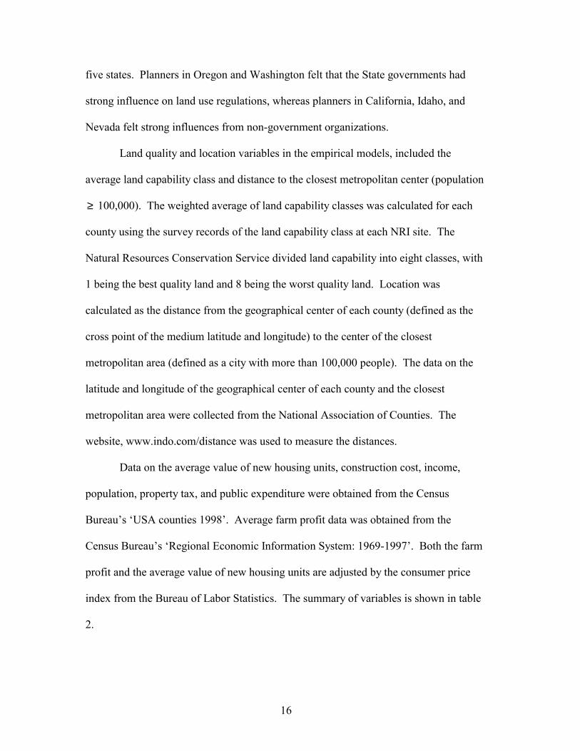
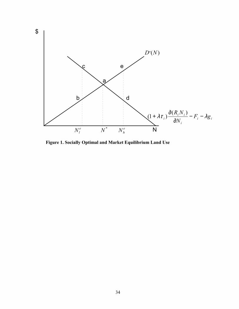
The first order condition for optimal land use is illustrated in figure 1. The

socially optimal level of land development, *N , obtained from equation (12), is where

the marginal benefit of development equals the marginal cost of development.

However, the developed area under the market equilibrium can be greater or less than

the socially optimal level of land development, resulting in a social welfare loss. If the

developed area under the market equilibrium elN is less than the socially optimal level

*N , the welfare loss is the area abc. If the developed area under the market

equilibrium is ehN , the welfare loss is the area ade. In both cases, a county government

can reduce the welfare loss by shifting the market equilibrium land use toward the

socially optimal land use in the form of land use regulations. A county government can

encourage development by reducing land use regulations and discourage development

by imposing more stringent land use regulations. Thus, the probability that land use

regulations will be imposed depends on the difference between the left and right hand

sides of (12), which is

),,,,,,,,,(Pr 1*

−Ψ= ttttttttxttt NDgYFp µτσϕ . (13)

From the first order condition of the county government�s maximization problem, we

obtain the government expenditure and property tax functions:

),,,,,,,,,( 1*

−Ψ= ttttttttxttt NDYFpgg τµϕσ , (14)

10

),,,,,,,,,,( 1*

−Ψ= ttttttttxttt NDgYFp µϕσττ (15)

which, together with the public budget constraint, determine the optimal level of public

expenditure and property taxes.

The Empirical Model

In the last section, we analyzed the theoretical interrelationships between land

use, land use regulations, and their fiscal impacts. In this section, we present an

empirical model of these interrelationships. Specifically, the interrelationships are

represented by the following simultaneous equations system with self-selection and

discrete dependent variables:

� Π⋅

Π⋅==≡

=

M

iit

jtjt

X

XjI

1

'

'

)exp(

)exp()Pr(Pr , j = 1, 2, 3, 4, (16)

sjtt

jt

jjsjt ZRN εβββ +⋅+⋅+= 210 , (17)

Rjtt

jt

jt

jjjt ZgR εγγτγγ +⋅+⋅+⋅+= 3210 , (18)

jtt

jt

jjjt Zg τεδδδτ +⋅+⋅+= 210 , (19)

gjtt

jt

jjjt Zg επτππ +⋅+⋅+= 210 , (20)

where j = 1, 2, 3, 4 represents the four degrees of land use regulations as defined in table 1,

tZ is a matrix of exogenous variables ),,,,,( 1 Ψ− ttttt YFN σµ , and gjt

jt

Rjt

sjt εεεε τ ,,, are

random error terms.

The degree of land use regulations is defined based on a comprehensive survey of

land use regulations in each county in five western states (California, Idaho, Nevada,

Oregon, and Washington). From the survey, we identified the 20 most important land use

regulations. Survey respondents were asked to evaluate the level of effectiveness of each

11

regulation on a scale of 1, 2, 3, 4, and 5 with 1 being not effective and 5 being most

effective. The sum of the level of effectiveness for all regulations in a county is defined as

an index of regulatory intensity. For example, a county with 20 land use regulations each

with level of effectiveness of 5, would have an index of 100. Counties with indexes greater

than 60 are classified as having �stringent land use regulations�, counties with indexes

greater than 30 and equal to or less than 60 are classified as having �moderate land use

regulations�, counties with indexes greater than 0 and equal to or less than 30 are classified

as having �low land use regulations�, and counties without any land use regulations are

defined as �no land use regulations�.

The equation system (16-20) is an extension of the polychotomous-choice

selectivity model as described in Lee (1983) and applied to agricultural policy analysis in

Wu and Babcock (1998). When any two equations of land demand, land supply, and

housing price are estimated, the other one would be determined. Here we choose to

estimate the land supply and housing price equations.

Maddala (1983, p. 242-245) describes a two-stage technique for estimating a

simultaneous model with discrete dependent variables. In the first stage, we estimate

the reduced form equations of (18), (19), and (20), using OLS:

jtt

jjt ZR 11 ν+⋅Π= (21)

jtt

jjt Z 22 ντ +⋅Π= (22)

jtt

jjt Zg 33 ν+⋅Π= (23)

We then use the predicted value of gR �,�,� τ to estimate the multinomial logit model in

(16) and use it to predict jrP� :

12

� ⋅Π

⋅Π=

=

M

iti

tjjt

X

X

1)�exp(

)�exp(rP� , j = 1, 2, 3, 4. (24)

which is then used to calculate jt

jt

jt rP�/)]rP�([� 1−Φ≡ φλ , j = 1, 2, 3, 4. The j

tλ� reflects

correction of self-selection bias (Lee, 1983). It is included in the model because

counties that adopt land use regulations may behave differently from a randomly

selected county with the same characteristics.

In the second stage, the parameters in the structural equations are determined by

estimating the following equations using OLS:

jt

jt

jt

jt

jjjt uZRN 13210

�� +⋅−⋅+⋅+= λββββ (25)

jt

jt

jt

jt

jt

jjjt uZgR 243210

�� +⋅−⋅+⋅+⋅+= λγγγτγγ (26)

jt

jt

jt

jt

jjjt uZg 33210

�� +⋅−⋅+⋅+= λδδδδτ (27)

jt

jt

jt

jt

jjjt uZg 43210

�� +⋅−⋅+⋅+= λππτππ (28)

Since the coefficients of the multinomial logit model are difficult to interpret, the

marginal effects of explanatory variables on the degree of regulation are determined

using

)Pr(PrPr 3

1� Π⋅−Π=

∂∂

=ii

ij

jj

X. (29)

This model can be used to estimate the effects of alternative degrees of land use

regulations on land development, housing price, public expenditure, and property tax.

Consider the public expenditure of a county with and without land use regulations, the

expected change in public expenditure due to the adoption of level of land use

regulation j is:

13

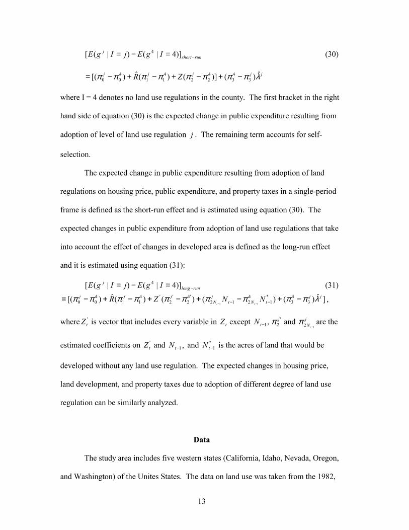
runshortj IgEjIgE −=−= )]4|()|([ 4 (30)

jjjjj ZR λππππππππ �)()]()(�)[( 343

422

411

400 −+−+−+−=

where I = 4 denotes no land use regulations in the county. The first bracket in the right

hand side of equation (30) is the expected change in public expenditure resulting from

adoption of level of land use regulation j . The remaining term accounts for self-

selection.

The expected change in public expenditure resulting from adoption of land

regulations on housing price, public expenditure, and property taxes in a single-period

frame is defined as the short-run effect and is estimated using equation (30). The

expected changes in public expenditure from adoption of land use regulations that take

into account the effect of changes in developed area is defined as the long-run effect

and it is estimated using equation (31):

runlongj IgEjIgE −=−= )]4|()|([ 4 (31)

]�)()()()(�)[( 343

*1

4212

'42

'2

'411

400 11

jjtNt

jN

jjj NNZRtt

λππππππππππ −+−+−+−+−= −− −−,

where 'tZ is vector that includes every variable in tZ except ,1−tN '

2jπ and j

Nt 12 −π are the

estimated coefficients on 'tZ and ,1−tN and *

1−tN is the acres of land that would be

developed without any land use regulation. The expected changes in housing price,

land development, and property taxes due to adoption of different degree of land use

regulation can be similarly analyzed.

Data

The study area includes five western states (California, Idaho, Nevada, Oregon,

and Washington) of the Unites States. The data on land use was taken from the 1982,

14

1987, and 1992 Natural Resource Inventories (NRI)1. The NRI collected land use data

at 800,000 randomly selected sites across the continental United States and divided land

use into twelve major categories (cultivated cropland, non-cultivated cropland,

pastureland, rangeland, forestland, urban and built-up land, and six other categories).

In this study, cultivated cropland, non-cultivated cropland, pastureland, and rangeland

are categorized as farmland and urban and built-up land is categorized as urban land.

The NRI survey assigns a weight called an expansion factor or �X� factor to each site

in the sample to determine the number of acres each sample site represents. The sum of

this value for all sites in a county equals the total county acreage.

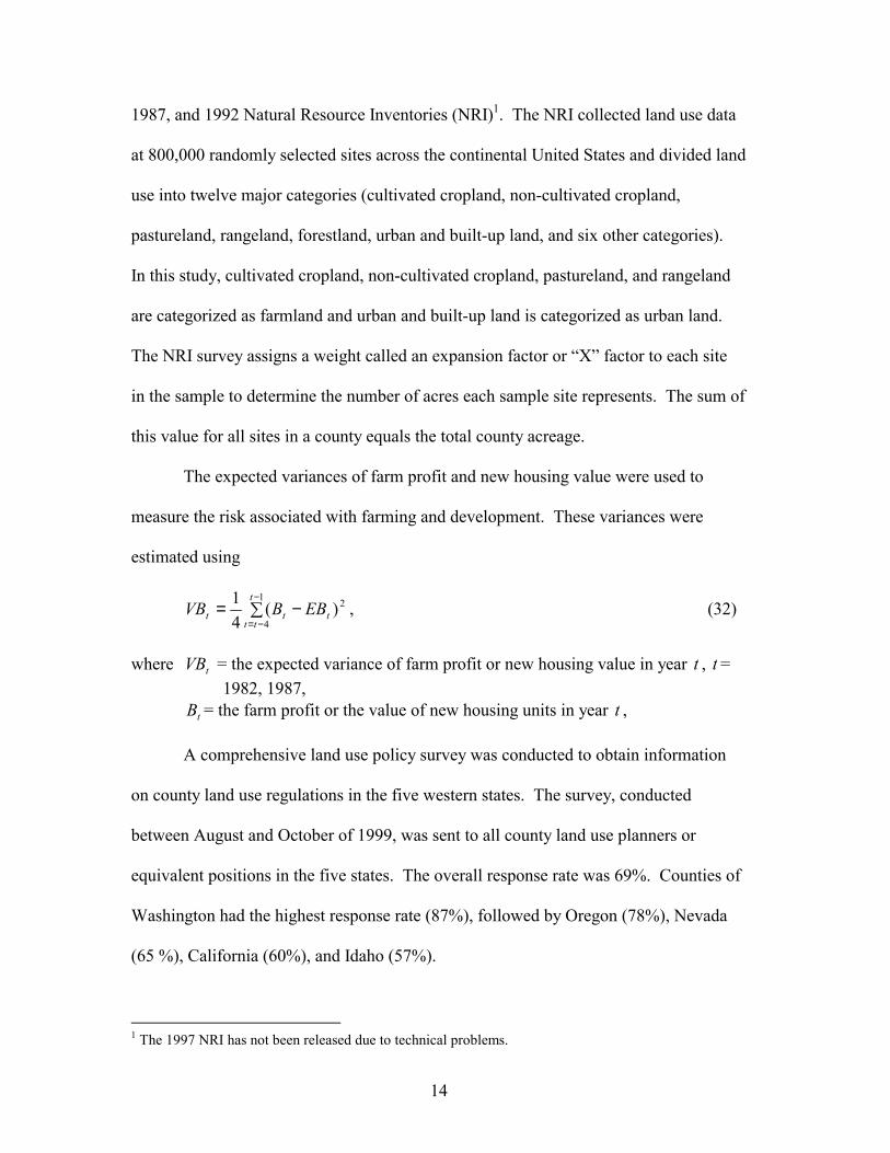
The expected variances of farm profit and new housing value were used to

measure the risk associated with farming and development. These variances were

estimated using

� −=−

−=

1

4

2)(4

1 t

ttttt EBBVB , (32)

where tVB = the expected variance of farm profit or new housing value in year t , t =

1982, 1987, tB = the farm profit or the value of new housing units in year t ,

A comprehensive land use policy survey was conducted to obtain information

on county land use regulations in the five western states. The survey, conducted

between August and October of 1999, was sent to all county land use planners or

equivalent positions in the five states. The overall response rate was 69%. Counties of

Washington had the highest response rate (87%), followed by Oregon (78%), Nevada

(65 %), California (60%), and Idaho (57%).

1 The 1997 NRI has not been released due to technical problems.

15

The survey results show that the most important land use policy goal of Nevada

counties was the promotion of industrial and commercial investment, while the counties

in other states were more concerned about the conservation of farmland, forestland, and

natural areas. All counties expressed a serious concern about urbanization. A county

comprehensive plan had been enacted in almost all of the counties in the five states

when the survey was conducted, however, the timing of the initial enactment varied

across counties. Extra territorial planning and zoning were popular in Idaho, urban

growth boundaries were popular in Oregon and Washington. Agricultural, residential,

forestry, conservation, open space, and steep slope zonings were popular throughout the

states, whereas performance zoning was used only in a limited number of counties.

Specification of minimum parcel sizes was popular in many counties, limits on

maximum parcel sizes was not.

Developer exaction and dedication was the most popular land acquisition

technique in many counties. Fee simple purchase and agricultural districts were

especially popular in California. Preferential property taxation for farmland and

forestland were the most popular incentive-based management techniques. Special

assessments were popular in Oregon, Washington, and California.

Environmental impact assessments were popular in Washington and California.

Regional fair sharing was especially popular in California. The planners predicted a

high possibility of conversion from farmland to residential land, especially in Idaho and

Nevada. Counties in California spent the largest amount of money on planning, while

counties in Idaho spent the least amount. However, the average share of money spent

on planning out of general fund for the entire county budget remained fairly close in the

16

five states. Planners in Oregon and Washington felt that the State governments had

strong influence on land use regulations, whereas planners in California, Idaho, and

Nevada felt strong influences from non-government organizations.

Land quality and location variables in the empirical models, included the

average land capability class and distance to the closest metropolitan center (population

≥ 100,000). The weighted average of land capability classes was calculated for each

county using the survey records of the land capability class at each NRI site. The

Natural Resources Conservation Service divided land capability into eight classes, with

1 being the best quality land and 8 being the worst quality land. Location was

calculated as the distance from the geographical center of each county (defined as the

cross point of the medium latitude and longitude) to the center of the closest

metropolitan area (defined as a city with more than 100,000 people). The data on the

latitude and longitude of the geographical center of each county and the closest

metropolitan area were collected from the National Association of Counties. The

website, www.indo.com/distance was used to measure the distances.

Data on the average value of new housing units, construction cost, income,

population, property tax, and public expenditure were obtained from the Census

Bureau�s �USA counties 1998�. Average farm profit data was obtained from the

Census Bureau�s �Regional Economic Information System: 1969-1997�. Both the farm

profit and the average value of new housing units are adjusted by the consumer price

index from the Bureau of Labor Statistics. The summary of variables is shown in table

2.

17

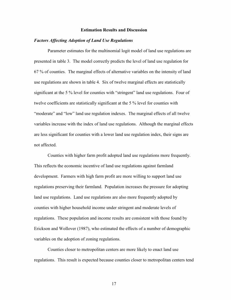
Estimation Results and Discussion

Factors Affecting Adoption of Land Use Regulations

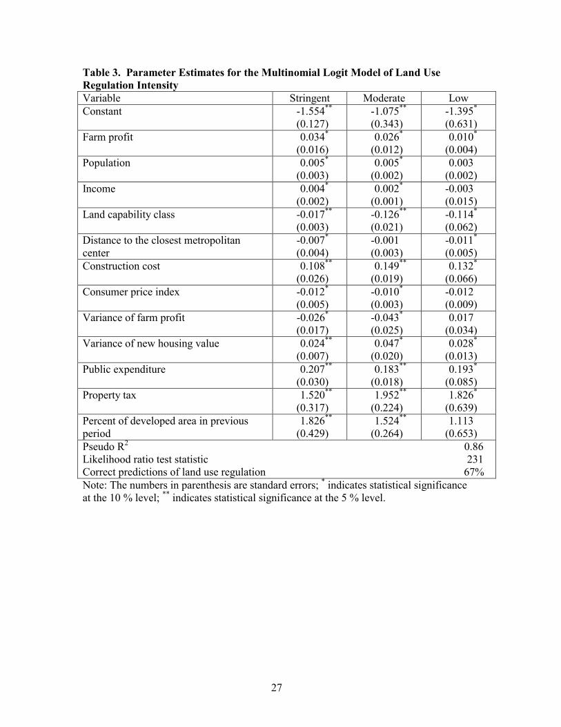
Parameter estimates for the multinomial logit model of land use regulations are

presented in table 3. The model correctly predicts the level of land use regulation for

67 % of counties. The marginal effects of alternative variables on the intensity of land

use regulations are shown in table 4. Six of twelve marginal effects are statistically

significant at the 5 % level for counties with �stringent� land use regulations. Four of

twelve coefficients are statistically significant at the 5 % level for counties with

�moderate� and �low� land use regulation indexes. The marginal effects of all twelve

variables increase with the index of land use regulations. Although the marginal effects

are less significant for counties with a lower land use regulation index, their signs are

not affected.

Counties with higher farm profit adopted land use regulations more frequently.

This reflects the economic incentive of land use regulations against farmland

development. Farmers with high farm profit are more willing to support land use

regulations preserving their farmland. Population increases the pressure for adopting

land use regulations. Land use regulations are also more frequently adopted by

counties with higher household income under stringent and moderate levels of

regulations. These population and income results are consistent with those found by

Erickson and Wollover (1987), who estimated the effects of a number of demographic

variables on the adoption of zoning regulations.

Counties closer to metropolitan centers are more likely to enact land use

regulations. This result is expected because counties closer to metropolitan centers tend

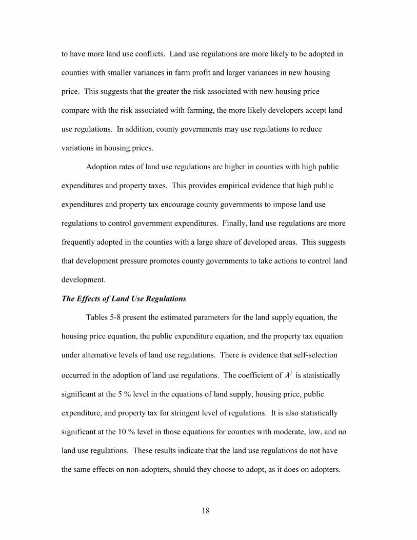
18

to have more land use conflicts. Land use regulations are more likely to be adopted in

counties with smaller variances in farm profit and larger variances in new housing

price. This suggests that the greater the risk associated with new housing price

compare with the risk associated with farming, the more likely developers accept land

use regulations. In addition, county governments may use regulations to reduce

variations in housing prices.

Adoption rates of land use regulations are higher in counties with high public

expenditures and property taxes. This provides empirical evidence that high public

expenditures and property tax encourage county governments to impose land use

regulations to control government expenditures. Finally, land use regulations are more

frequently adopted in the counties with a large share of developed areas. This suggests

that development pressure promotes county governments to take actions to control land

development.

The Effects of Land Use Regulations

Tables 5-8 present the estimated parameters for the land supply equation, the

housing price equation, the public expenditure equation, and the property tax equation

under alternative levels of land use regulations. There is evidence that self-selection

occurred in the adoption of land use regulations. The coefficient of jλ is statistically

significant at the 5 % level in the equations of land supply, housing price, public

expenditure, and property tax for stringent level of regulations. It is also statistically

significant at the 10 % level in those equations for counties with moderate, low, and no

land use regulations. These results indicate that the land use regulations do not have

the same effects on non-adopters, should they choose to adopt, as it does on adopters.

19

The parameter estimates for counties with stringent land use regulations are generally

greater than for those with less stringent regulations in all four equations. This reflects

that under stringent land use regulations, land supply, housing price, public

expenditure, and property tax are more sensitive to variables affecting them.

The results in table 5 indicate that developers are more likely to develop in

counties with higher land quality, higher income, and larger population. They develop

more land in counties closer to metropolitan areas. Higher housing prices increase the

supply of housing and thus land development; however, housing supply is negatively

correlated with farm profit since farm profit is an opportunity cost of land development.

The positive coefficients on variance of farm profit and negative coefficients on

variance of new housing prices in the land supply equations indicate that developers are

more likely to develop when facing high risks and uncertainties of farm profit and less

likely to develop when facing high risks and uncertainties of housing price.

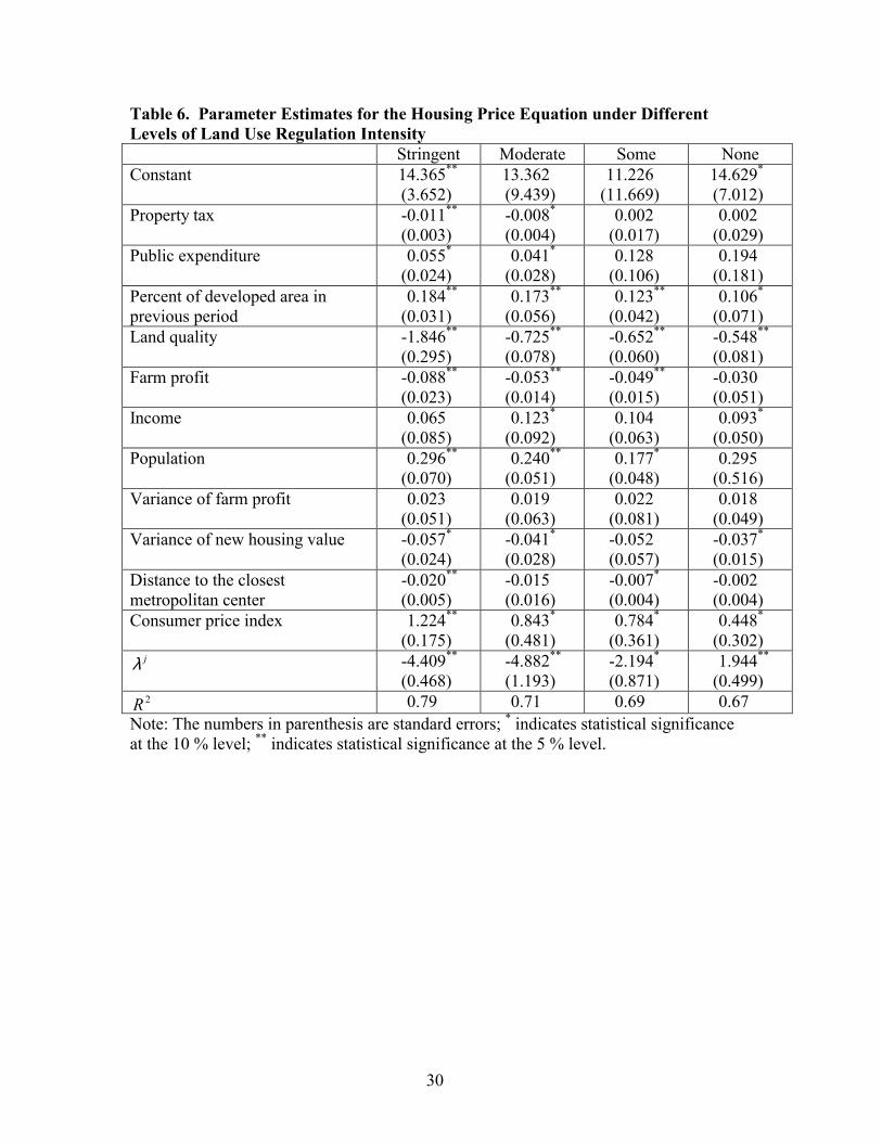
Parameter estimates for the housing price equation are shown in table 6. Seven

of twelve coefficients under stringent regulation are statistically significant at the 5 %

level. Only two of twelve coefficients are statistically significant at the 5 % level under

no regulation. The coefficients on the distance to a metropolitan center and property

taxes were not statistically significant at the 10% level under no regulation but they

were statistically significant at the 5 % level under stringent regulations. This suggests

that counties with stringent regulations are likely to be located near a metropolitan

center where housing prices are significantly affected by both the distance to the

metropolitan center and property taxes.

20

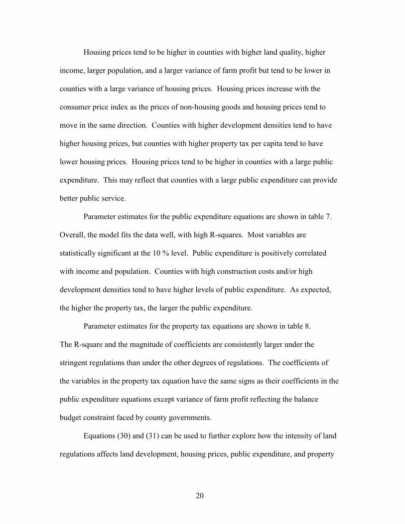
Housing prices tend to be higher in counties with higher land quality, higher

income, larger population, and a larger variance of farm profit but tend to be lower in

counties with a large variance of housing prices. Housing prices increase with the

consumer price index as the prices of non-housing goods and housing prices tend to

move in the same direction. Counties with higher development densities tend to have

higher housing prices, but counties with higher property tax per capita tend to have

lower housing prices. Housing prices tend to be higher in counties with a large public

expenditure. This may reflect that counties with a large public expenditure can provide

better public service.

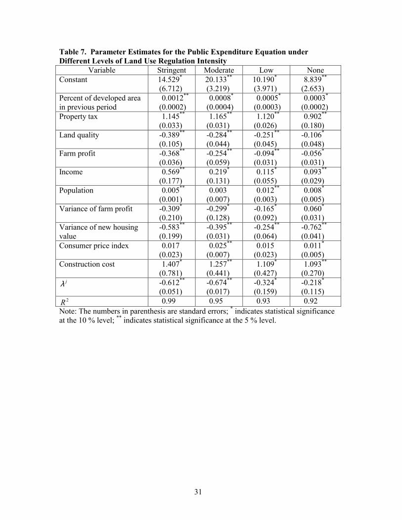
Parameter estimates for the public expenditure equations are shown in table 7.

Overall, the model fits the data well, with high R-squares. Most variables are

statistically significant at the 10 % level. Public expenditure is positively correlated

with income and population. Counties with high construction costs and/or high

development densities tend to have higher levels of public expenditure. As expected,

the higher the property tax, the larger the public expenditure.

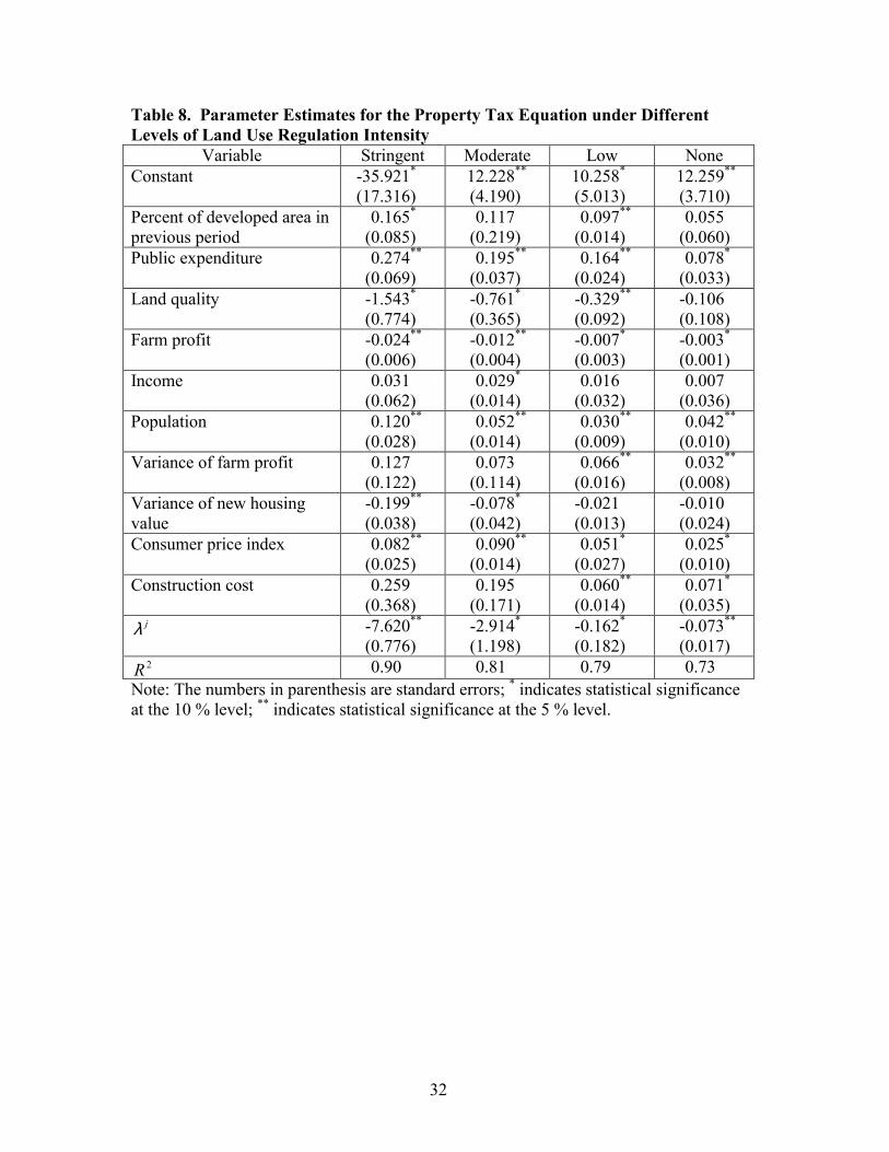
Parameter estimates for the property tax equations are shown in table 8.

The R-square and the magnitude of coefficients are consistently larger under the

stringent regulations than under the other degrees of regulations. The coefficients of

the variables in the property tax equation have the same signs as their coefficients in the

public expenditure equations except variance of farm profit reflecting the balance

budget constraint faced by county governments.

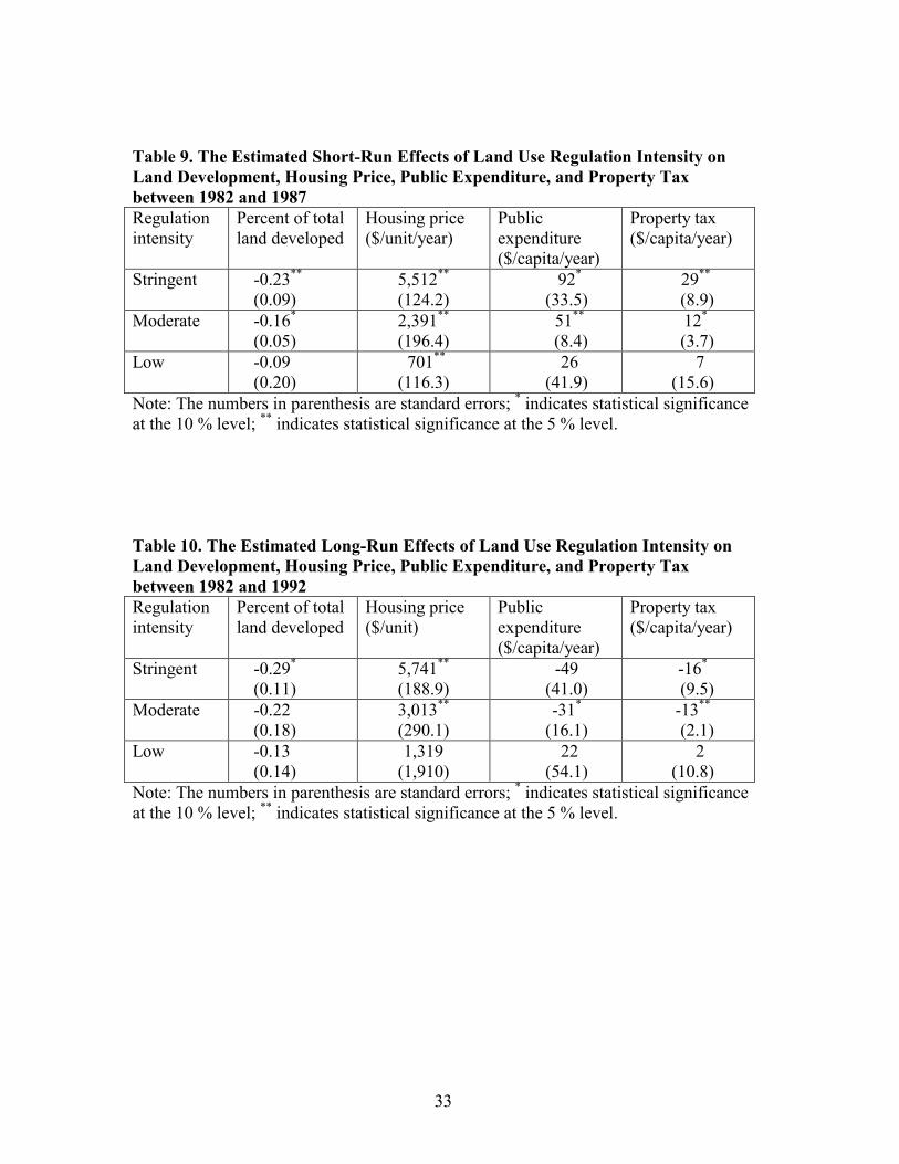
Equations (30) and (31) can be used to further explore how the intensity of land

regulations affects land development, housing prices, public expenditure, and property

21

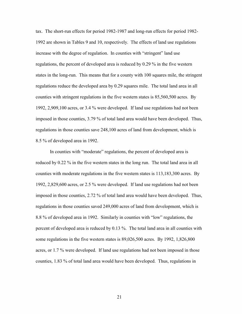
tax. The short-run effects for period 1982-1987 and long-run effects for period 1982-

1992 are shown in Tables 9 and 10, respectively. The effects of land use regulations

increase with the degree of regulation. In counties with �stringent� land use

regulations, the percent of developed area is reduced by 0.29 % in the five western

states in the long-run. This means that for a county with 100 squares mile, the stringent

regulations reduce the developed area by 0.29 squares mile. The total land area in all

counties with stringent regulations in the five western states is 85,560,500 acres. By

1992, 2,909,100 acres, or 3.4 % were developed. If land use regulations had not been

imposed in those counties, 3.79 % of total land area would have been developed. Thus,

regulations in those counties save 248,100 acres of land from development, which is

8.5 % of developed area in 1992.

In counties with �moderate� regulations, the percent of developed area is

reduced by 0.22 % in the five western states in the long run. The total land area in all

counties with moderate regulations in the five western states is 113,183,300 acres. By

1992, 2,829,600 acres, or 2.5 % were developed. If land use regulations had not been

imposed in those counties, 2.72 % of total land area would have been developed. Thus,

regulations in those counties saved 249,000 acres of land from development, which is

8.8 % of developed area in 1992. Similarly in counties with �low� regulations, the

percent of developed area is reduced by 0.13 %. The total land area in all counties with

some regulations in the five western states is 89,026,500 acres. By 1992, 1,826,800

acres, or 1.7 % were developed. If land use regulations had not been imposed in those

counties, 1.83 % of total land area would have been developed. Thus, regulations in

22

those counties save 115,700 acres of land from development, which is 6.3 % of

developed area in 1992.

All land use regulations in the five western states saved an estimated total of

458,000 acres (6.6 % of developed area in 1992) in the short-run and 612,800 acres (8.8

% of developed area in 1992) in the long-run. However, in counties with the most

stringent land use regulations, the average new housing price increased by $5,741 per

unit in the long-run. The average new housing price was $146,000 in 1982, thus the

stringent land use regulations increased new housing prices by 3.9 % compared to no

land use regulations.

Under stringent regulations, public expenditure increased by the largest amount

($92 per capita) in the short-run. The average public expenditure was $1,320 per capita

in 1982, thus the stringent regulations increased public expenditure by 7.0 % in the

short-run. However, in the long-run, land use regulations reduced public expenditure

by $49 per capita under stringent regulations, a 3.7 % decrease compared to no

regulations. Property tax also increased by the largest amount ($29 per capita) under

the stringent regulation in the short-run. However, in the long-run, land use regulations

reduced property tax by $16 per capita under stringent regulation.

The different short-run vs. long-run effects on public expenditure and property

taxes suggest that in the short-run, county governments raise property taxes to cover the

increased public expenditure needed to develop and implement land use regulations,

whereas, in the long-run land use regulations reduce public expenditure and property

taxes by reducing the extent of developed areas. In summary, in the long-run land use

regulation reduced the amount of land developed, long-run public expenditure, and

23

property tax; however, not without higher long-run housing prices, and short-run

increases in public expenditure and property tax.

Conclusions

Measuring effects of land use regulations is becoming increasingly important as

more communities exercise land use regulations. Previous studies on land use

regulations have focused on a single land use regulation, treating all others as given and

exogenously determined. They also have neglected interactions among residential

development, land use regulations, and public finance (public expenditure and property

tax). In this study a simultaneous equations system with self-selection and discrete

dependent variables is used to estimate adoption decisions of land use regulations and

their impacts on land use, public expenditure, and property tax.

The method is applied to land use regulation decisions in five western states

using data from a comprehensive survey on land use regulations, the 1982, 1987, and

1992 National Resources Inventories, and other USDA publications. The results

indicate that conversion of farmland and open space to development along with high

public expenditure and property taxes promote county governments to impose more

stringent land use regulations. More stringent land use regulations, in turn, reduce land

development, long-run public expenditure, and property tax; however, not without

higher long-run housing prices and short-run increases in public expenditure and

property tax. The results also show that land use regulations, land development, public

expenditure, and property tax all are significantly affected by population, geographic

location, land quality, housing rent, and risks and costs of development.

24

References

Alig, R. J. and R. G. Healy. �Urban and Built-Up Land Area Changes in the United States: An Empirical Investigation of Determinants� Land Economics 63(1987): 215-226..

Bockstael, N., R. Costanza, I. Strand, W. Boynton, K. Bell, and L. Waigner.

�Ecological Economic Modeling and Valuation of Ecosystems.� Ecological Economics 14(1995): 143-159.

Chicoine, D. L. �Farmland Values at the Urban Fringe: An Analysis of Sales Prices.�

Land Economics 57(1981): 353-362. Davis, O. A. �Economic Elements in Municipal Zoning Decisions.� Land Economics

39(1963): 375-386. Epple, D., T. Romer, and R. Filmore. �Community Development with Endogenous

Land Use Controls.� Journal of Public Economics 35(1988):133-162. Epple, D. and H. Sieg. �Estimation Equilibrium Models of Local Jurisdictions.�

Journal of Political Economics 107(1999): 645-681. Erickson, R. A. and D. R. Wollover. �Local Tax Burdens and the Supply of Business

Sites in Suburban Municipalities.� Journal of Regional Science 27(1987): 25-37. Fischel, W. A. �A property Rights Approach to Municipal Zoning.� Land Economics

54 (1978): 64-81. Greene, W. H. Econometric Analysis. New Jersey: Prentice Hall, 1997. Hardie, I. W. and P. J. Parks. �Land Use with Heterogeneous Land Quality: An

Application of an Area Base Model.� American Journal of Agricultural Economics 79 (1997): 299-310.

Henderson, V. �Community Development: The Effect of Growth and Uncertainty.�

American Economic Review 70(1980): 894-910. Hushak, L. J. and K. Sadr. �A Spatial Model of Land Market Behavior,� American

Journal of Agricultural Economics 61(1979): 697-701. Lee, L. F. �Generalized Econometric Models with Selectivity.� Econometrica

51(1983): 507-512. Levine, N. �The Effects of Local Growth Controls on Regional Housing Production

and Population Redistribution in California, Urban Studies.� 36(1999): 2047-2068.

25

Maddala, G. S. Limited Dependent and Qualitative Variables in Econometrics. CambrIdahoge: CambrIdahoge University Press, 1983.

McDonald, J. F. and D. P. McMillen. �Land Values, Land Use, and the First Chicago

Zoning Ordinances.� Journal of Real Estate Finance and Economics 16(1998): 135-150.

McMillen, D. P. and J. F. McDonald. �Selectivity Bias in Urban Land Value

Functions.� Land Economics 65(1989): 341-351. McMillen, D. P. and J. F. McDonald. �Urban Land Value Function with Endogenous

Zoning.� Land Economics 29(1991): 14-27. Mills, E. �Economic Analysis of Urban Land-Use Controls� in Current Issues in Urban

Economics. P. Mieszkowski and M. Straszheim, Eds. Baltimore: Johns Hopkins University Press, 1979.

Phillips J. and E. Goodstein. �Growth Management and Housing Prices: The case of

Portland, Oregon.� Contemporary Economic Policy 18 (2000): 334-344. Pogodzinski, J. M. and T. R. Sass. �The Theory and Estimation of Endogenous

Zoning.� Regional Science and Urban Economics 24(1994): 601-630. Rolleston, B. S. �Determinants of Restrictive Suburban Zoning: An Empirical

Analysis.� Journal of Urban Economics 21(1987): 1-21. Shlay, A. B. and P. H. Rossi. �Keeping Up the Neighborhood: Estimating Net Effects

of Zoning.� American Sociological Review 46(1981): 703-719. Wall, B. R. �Trends in Commercial Timberland Area in the United States by State and

Ownership, 1952-77, with Projections to 2030,� General Technical Report, Pacific Northwest Forest and Range Experiment Station, Portland OR(1981).

Wallace, N.W. �The Market Effects of Zoning Undeveloped Land: Does Zoning

Follow the Market?� Journal of Urban Economics 23(1988): 307-326. Wu, J. and B. A. Babcock. �The Choice of Tillage, Rotation, and Soil Testing

Practices: Economic and Environmental Implications.� American Journal of Agricultural Economics 80(1998): 494-511.

26

Table 1. The Intensity of Land Use Regulation in the Five Western States Category Index of intensity of land use regulations (I) % of Counties Stringent I ≥ 60 31 % Moderate 30 ≤ I < 60 33 % Low 0 < I < 30 25 % No Regulations 0 11 %

Table 2. Definition of Variables

Variables Mean Standard Deviation

Definition

Endogenous Variables: Percent of total land developed

1.87

0.22

Percent of total land developed (%)

New housing price 159.0 91.5 Value of private new housing units ($1,000) Property tax 436.0 67.0 Property tax per capita ($) Public expenditure

1859.0 616.0 Public expenditure per capita ($)

Exogenous Variables: Farm profit

8.2

15.9

Farm profit per acre ($)

Population 0.2 0.9 Population per acre Income 15.6 4.0 Income per capita ($ 1,000) Land capability class 5.2 0.9 Weighted average of land capability class

with 1 being the best land and 8 being the worst land

Distance to the closest metropolitan center

80.0 52.6 Distance from the geographic center of a county to the closest metropolitan center (population ≥ 100,000) (mile)

Construction cost 75.0 28.8 Construction cost as recorded on the building permit ($1,000)

Consumer price index 127.0 13.0 Consumer price index Variance of farm profit 169.3 1,006.1 Variance of farm profit at the beginning of

the period Variance of new housing value

353.5 1,949.1 Variance of housing value at the beginning of the period

27

Table 3. Parameter Estimates for the Multinomial Logit Model of Land Use Regulation Intensity Variable Stringent Moderate Low Constant -1.554**

(0.127) -1.075**

(0.343) -1.395*

(0.631) Farm profit 0.034*

(0.016) 0.026*

(0.012) 0.010*

(0.004) Population 0.005*

(0.003) 0.005*

(0.002) 0.003

(0.002) Income 0.004*

(0.002) 0.002*

(0.001) -0.003

(0.015) Land capability class -0.017**

(0.003) -0.126**

(0.021) -0.114*

(0.062) Distance to the closest metropolitan center

-0.007*

(0.004) -0.001

(0.003) -0.011*

(0.005) Construction cost 0.108**

(0.026) 0.149**

(0.019) 0.132*

(0.066) Consumer price index -0.012*

(0.005) -0.010*

(0.003) -0.012

(0.009) Variance of farm profit -0.026*

(0.017) -0.043*

(0.025) 0.017

(0.034) Variance of new housing value 0.024**

(0.007) 0.047*

(0.020) 0.028*

(0.013) Public expenditure 0.207**

(0.030) 0.183**

(0.018) 0.193*

(0.085) Property tax 1.520**

(0.317) 1.952**

(0.224) 1.826*

(0.639) Percent of developed area in previous period

1.826**

(0.429) 1.524**

(0.264) 1.113

(0.653) Pseudo R2 0.86 Likelihood ratio test statistic 231 Correct predictions of land use regulation 67% Note: The numbers in parenthesis are standard errors; * indicates statistical significance at the 10 % level; ** indicates statistical significance at the 5 % level.

28

Table 4. The Marginal Effects of Alternative Variables on the Intensity of Land Use Regulation Variable Stringent Moderate Low Farm profit 0.0043*

(0.0022) 0.0039*

(0.0017) 0.0031*

(0.0012) Population 0.0013*

(0.0005) 0.0010*

(0.0006) 0.0006

(0.0005) Income 0.0007*

(0.0003) 0.0005

(0.0009) -0.0003

(0.0024) Land capability class 0.0053*

(0.0038) 0.0045*

(0.0021) 0.0038*


-0.0008**

(0.0002) -0.0007*

(0.0004) -0.0001 (0.0018)

Construction cost 0.0275**

(0.0041) 0.0175*

(0.0084) 0.0098**

(0.0010) Consumer price index 0.0012

(0.0007) 0.0010*

(0.0004) 0.0001


(0.0061) -0.0088**

(0.0026) -0.0069*

(0.0025) Variance of new housing value 0.0033**

(0.0008) 0.0032*

(0.0018) 0.0025


(0.0031) 0.0135**

(0.0027) 0.0105**

(0.0031) Property tax 0.1126**

(0.0210) 0.1105**

(0.0184) 0.1021**


0.1942**

(0.0031) 0.1935**

(0.0046) 0.1654**

(0.0109) Note: The numbers in parenthesis are standard errors; * indicates statistical significance at the 10 % level; ** indicates statistical significance at the 5 % level.

29

Table 5. Parameter Estimates for the Supply Equation of Land Development under Different Levels of Land Use Regulation Intensity

Variable Stringent Moderate Low None Constant 0.193**

(0.018) 0.156**

(0.035) 0.103**

(0.029) 0.056*

(0.020) Land quality -0.013**

(0.002) -0.008*

(0.004) -0.007

(0.009) -0.002

(0.031) Farm profit -0.216**

(0.061) -0.185**

(0.043) -0.029

(0.033) -0.019**

(0.002) Variance of farm profit 0.014*

(0.005) 0.008*

(0.004) 0.006**

(0.001) 0.001

(0.025) Variance of new housing value

-0.002*

(0.001) -0.002*

(0.001) -0.001

(0.004) -0.001*

(0.001) Income 0.012**

(0.003) 0.007*

(0.004) 0.002*

(0.001) 0.001

(0.018) Population 0.0005**

(0.0001) 0.0006**

(0.0001) 0.0004

(0.0012) 0.0002*


-0.0015*

(0.0008) -0.0011*

(0.0004) -0.0008*

(0.0003) -0.0005*

(0.0002) New housing price 0.0006**

(0.0002) 0.0005*

(0.0003) 0.0001

(0.0010) 0.0001

(0.0022) jλ -0.128**

(0.024) -0.095**

(0.013) -0.0045**

(0.0009) -0.0029*

(0.0016) 2R 0.89 0.86 0.84 0.77

Note: The numbers in parenthesis are standard errors; * indicates statistical significance at the 10 % level; ** indicates statistical significance at the 5 % level.

30

Table 6. Parameter Estimates for the Housing Price Equation under Different Levels of Land Use Regulation Intensity

Stringent Moderate Some None Constant 14.365**

(3.652) 13.362 (9.439)

11.226

(11.669) 14.629*

(7.012) Property tax -0.011**

(0.003) -0.008*

(0.004) 0.002

(0.017) 0.002

(0.029) Public expenditure 0.055*

(0.024) 0.041*

(0.028) 0.128

(0.106) 0.194


0.184**

(0.031) 0.173**

(0.056) 0.123**

(0.042) 0.106*

(0.071) Land quality -1.846**

(0.295) -0.725**

(0.078) -0.652**

(0.060) -0.548**

(0.081) Farm profit -0.088**

(0.023) -0.053**

(0.014) -0.049**

(0.015) -0.030

(0.051) Income 0.065

(0.085) 0.123*

(0.092) 0.104

(0.063) 0.093*

(0.050) Population 0.296**

(0.070) 0.240**

(0.051) 0.177*

(0.048) 0.295

(0.516) Variance of farm profit 0.023

(0.051) 0.019

(0.063) 0.022

(0.081) 0.018

(0.049) Variance of new housing value -0.057*

(0.024) -0.041*

(0.028) -0.052

(0.057) -0.037*


-0.020**

(0.005) -0.015

(0.016) -0.007*

(0.004) -0.002

(0.004) Consumer price index 1.224**

(0.175) 0.843*

(0.481) 0.784*

(0.361) 0.448*

(0.302) jλ -4.409**

(0.468) -4.882**

(1.193) -2.194*

(0.871) 1.944**

(0.499) 2R 0.79 0.71 0.69 0.67


31

Table 7. Parameter Estimates for the Public Expenditure Equation under Different Levels of Land Use Regulation Intensity

Variable Stringent Moderate Low None Constant 14.529*

(6.712) 20.133**

(3.219) 10.190*

(3.971) 8.839**


0.0012**

(0.0002) 0.0008*

(0.0004) 0.0005*

(0.0003) 0.0003*

(0.0002) Property tax 1.145**

(0.033) 1.165**

(0.031) 1.120**

(0.026) 0.902**

(0.180) Land quality -0.389**

(0.105) -0.284**

(0.044) -0.251**

(0.045) -0.106*

(0.048) Farm profit -0.368**

(0.036) -0.254**

(0.059) -0.094**

(0.031) -0.056*

(0.031) Income 0.569**

(0.177) 0.219*

(0.131) 0.115*

(0.055) 0.093**

(0.029) Population 0.005**

(0.001) 0.003

(0.007) 0.012**

(0.003) 0.008*


(0.210) -0.299*

(0.128) -0.165*

(0.092) 0.060*


-0.583**

(0.199) -0.395**

(0.031) -0.254**

(0.064) -0.762**

(0.041) Consumer price index 0.017

(0.023) 0.025**

(0.007) 0.015

(0.023) 0.011*

(0.005) Construction cost 1.407*

(0.781) 1.257**

(0.441) 1.109*

(0.427) 1.093**

(0.270) jλ -0.612**

(0.051) -0.674**

(0.017) -0.324*

(0.159) -0.218*

(0.115) 2R 0.99 0.95 0.93 0.92


32

Table 8. Parameter Estimates for the Property Tax Equation under Different Levels of Land Use Regulation Intensity

Variable Stringent Moderate Low None Constant -35.921*

(17.316) 12.228**

(4.190) 10.258*

(5.013) 12.259**


0.165*

(0.085) 0.117

(0.219) 0.097**

(0.014) 0.055


(0.069) 0.195**

(0.037) 0.164**

(0.024) 0.078*

(0.033) Land quality -1.543*

(0.774) -0.761*

(0.365) -0.329**

(0.092) -0.106

(0.108) Farm profit -0.024**

(0.006) -0.012**

(0.004) -0.007*

(0.003) -0.003*

(0.001) Income 0.031

(0.062) 0.029*

(0.014) 0.016

(0.032) 0.007

(0.036) Population 0.120**

(0.028) 0.052**

(0.014) 0.030**

(0.009) 0.042**

(0.010) Variance of farm profit 0.127

(0.122) 0.073

(0.114) 0.066**

(0.016) 0.032**


-0.199**

(0.038) -0.078*

(0.042) -0.021

(0.013) -0.010

(0.024) Consumer price index 0.082**

(0.025) 0.090**

(0.014) 0.051*

(0.027) 0.025*

(0.010) Construction cost 0.259

(0.368) 0.195

(0.171) 0.060**

(0.014) 0.071*

(0.035) jλ -7.620**

(0.776) -2.914*

(1.198) -0.162*

(0.182) -0.073**

(0.017) 2R 0.90 0.81 0.79 0.73


33

Table 9. The Estimated Short-Run Effects of Land Use Regulation Intensity on Land Development, Housing Price, Public Expenditure, and Property Tax between 1982 and 1987 Regulation intensity

Percent of total land developed

Housing price ($/unit/year)

Public expenditure ($/capita/year)

Property tax ($/capita/year)

Stringent -0.23**

(0.09) 5,512**

(124.2) 92*

(33.5) 29**

(8.9) Moderate -0.16*

(0.05) 2,391**

(196.4) 51**

(8.4) 12*

(3.7) Low -0.09

(0.20) 701**

(116.3) 26

(41.9) 7


Table 10. The Estimated Long-Run Effects of Land Use Regulation Intensity on Land Development, Housing Price, Public Expenditure, and Property Tax between 1982 and 1992 Regulation intensity

Percent of total land developed

Housing price ($/unit)

Public expenditure ($/capita/year)

Property tax ($/capita/year)

Stringent -0.29*

(0.11) 5,741**

(188.9) -49

(41.0) -16*

(9.5) Moderate -0.22

(0.18) 3,013**

(290.1) -31*

(16.1) -13**

(2.1) Low -0.13

(0.14) 1,319

(1,910) 22

(54.1) 2


34

N

$

a

b

c e

d

*NelN e

hN

)(ND ′

iii

iii gF

N

NR λλτ −−∂

∂+

)()1(

Figure 1. Socially Optimal and Market Equilibrium Land Use

Documents

Measuring Interactions among Urban Development, Land Use Regulations, and Public Finance