UC BerkeleyRecent Work

TitleMeasuring Market Power in the Ready-to-Eat Cereal Industry

Permalinkhttps://escholarship.org/uc/item/7cm5p858

AuthorNevo, Aviv

Publication Date1999-03-01

eScholarship.org Powered by the California Digital LibraryUniversity of California

Working Paper No. CPC99-01

Measuring Market Power in the Ready-to-Eat Cereal Industry

Aviv NevoEconomics Department, University of California

March 1999

Keywords: Discrete choice models, random coefficients, product differentiation, ready-to-eatcereal industry, market power, price competition

Abstract:The ready-to-eat cereal industry is characterized by high concentration, high price-cost margins,large advertising-to-sales ratios, and numerous introductions of new products. Previousresearchers have concluded that the ready-to-eat cereal industry is a classic example of anindustry with nearly collusive pricing behavior and intense non-price competition. This paperempirically examines this conclusion. In particular, I estimate price-cost margins, but moreimportantly I am able empirically to separate these margins into three sources: (1) that which isdue to product differentiation; (2) that which is due to multi-product firm pricing; and (3) that due topotential price collusion. The results suggest that given the demand for different brands of cereal,the first two effects explain most of the observed price-cost markups. I conclude that prices in theindustry are consistent with non-collusive pricing behavior, despite the high price-cost margins.Leading firms are able to maintain a portfolio of differentiated products and influence theperceived product quality. It is these two factors that lead to high price-cost margins.

__________________________This paper is based on various chapters of my 1997 Harvard University Ph. D. dissertation. Special thanks tomy advisors, Gary Chamberlain, Zvi Griliches and Michael Whinston for guidance and support. I wish tothank Ronald Cotterill, the director of the Food Marketing Policy Center in the University of Connecticut, forallowing me to use his data. I am grateful to Steve Berry, Ernst Berndt, Tim Bresnahan, David Cutler, JerryHausman, Igal Hendel, Kei Hirano, John Horn, Joanne McLean, Ariel Pakes, Rob Porter, Jim Powell, Johnvan Reenen, Richard Schmalensee, Sadek Wahba, Frank Wolak, Catherine Wolfram, the editor, threeanonymous referees, and participants in several seminars for comments and suggestions. Excellentresearch assistance was provided by Anita Lopez. Financial support from the Graduate School FellowshipFund at Harvard University, the Alfred P. Sloan Doctoral Dissertation Fellowship Fund, and the UC-BerkeleyCommittee on Research Junior Faculty Fund is gratefully acknowledged. Address for correspondence, 549Evans Hall #3880,Department of Economics, Berkeley, CA 94720-3880, e-mail: nevo@ econ. berkeley. eduThis paper is available on-line at http://www.haas.berkeley.edu/groups/cpc/pubs/Publications.html

2For example, Scherer (1982) argues that "...the cereal industry’s conduct fits well the model of pricecompetition-avoiding, non-price competition-prone oligopoly" (pg. 189).

1

1. INTRODUCTION

The ready-to-eat (RTE) cereal industry is characterized by high concentration, high

price-cost margins, large advertising-to-sales ratios and aggressive introduction of new products.

These facts have made this industry a classic example of a concentrated differentiated-products

industry in which price competition is approximately cooperative and rivalry is channeled into

advertising and new product introduction.2 This paper examines these conclusions regarding

price competition in the RTE cereal industry. In particular, I estimate the true economic price-

cost margins (PCM) in the industry and empirically distinguish between three sources of these

margins. The first source is the firms’ ability to differentiate its brands from those of its

competition. The second is the portfolio effect; if two brands are perceived as imperfect

substitutes, a firm producing both would charge a higher price than two separate manufacturers.

Finally, the main players in the industry could engage in price collusion.

My general strategy is to model demand as a function of product characteristics,

heterogeneous consumer preferences, and unknown parameters. Using data rarely available for

academic research, I extend recent developments in techniques for estimating demand and

supply in industries with closely related products (see Bresnahan, 1981, 1987; Berry, 1994;

Berry, Levinsohn, and Pakes, henceforth BLP, 1995) to estimate demand parameters. These

estimates are used to compute the PCM implied by three hypothetical industry structures: single-

product firms; the current structure (i.e., a few firms with many brands each); and a multi-brand

monopolist producing all brands. The markup in the first structure is due only to product-

differentiation. In the second case the markup also includes the multi-product firm portfolio

effect. Finally, the last structure produces the markups based on joint ownership, or full

3This assumption is similar to the one made in Hausman (1996), although our setups differ substantially.

2

collusion. I choose among the three conduct models by comparing the PCM predicted by them

to observed PCM. Despite the fact that I observe only a crude measure of actual PCM, I am still

able to distinguish between the markups predicted by these models.

The results suggest that the markups implied by the current industry structure, under a

Nash-Bertrand pricing game, match the observed PCM. If we take Nash-Bertrand prices as the

non-collusive benchmark, then even with PCM higher than 45% we can conclude that pricing in

the RTE cereal industry is approximately non-collusive. High PCM are not due to lack of price

competition, but are due to consumers’ willingness to pay for their favorite brand, and pricing

decisions by firms that take into account substitution between their own brands. To the extent

that there is any market power in this industry, it is due to the firms’ ability to maintain a

portfolio of differentiated products and influence perceived product quality through advertising.

The exercise relies on the ability to consistently estimate demand. I use a three-

dimensional panel of quantities and prices for 25 brands of cereal in up to 65 U.S. cities over a

period of 20 quarters, collected using scanning devices in a representative sample of

supermarkets. The estimation has to deal with two challenges: (1) the correlation between prices

and brand-city-quarter specific demand shocks, which are included in the econometric error

term, and (2) the large number of own- and cross-price elasticities implied by the large number

of products. I deal with the first challenge by exploiting the panel structure of the data. The

identifying assumption is that, controlling for brand-specific means and demographics, city-

specific demand shocks are independent across cities.3 Given this assumption, a demand shock

for a particular brand will be independent of prices of the same brand in other cities. Due to

common regional marginal cost shocks, prices of a brand in different cities within a region will

3

be correlated, and therefore can be used as valid instrumental variables. However, there are

several reasons why this identifying assumption might be invalid. For this reason I also explore

the use of observed variation in city-specific marginal costs. Not only are the demand estimates

from these two assumptions essentially identical, they are also similar to estimates obtained

using different data sets and alternative identifying assumptions.

The second difficulty is to estimate the large number of substitution parameters implied

by the numerous products in this industry. In this paper I overcome this difficulty by following

the discrete-choice literature (for example see McFadden, 1973, 1978, 1981; Cardell, 1989;

Berry ,1994; or BLP). I follow closely the method proposed by Berry (1994) and BLP, but

using the richness of my panel data I am able to combine panel data techniques with this method

and add to it in several ways. First, the method is applied to RTE cereal in which one might

doubt the ability of observed product characteristics to explain utility. By adding a brand fixed

effect I control for unobserved quality for which previous work had to instrument. Potential

difficulties with identifying all the parameters are solved using a minimum-distance procedure,

as in Chamberlain (1982). Second, most previous work assumed that observed brand

characteristics are exogenous and identified demand parameters using this assumption, which is

not consistent with a broader model in which brand characteristics are chosen by firms that

account for consumer preferences. The identifying assumption used here is consistent with this

broader model. Third, I model heterogeneity as a function of the empirical non-parametric

distribution of demographics, thereby partially relaxing the parametric assumptions previously

used.

The rest of the paper is organized as follows. Section 2 gives a short description of the

industry. In Section 3 I outline the empirical model and discuss the implications of different

4A full account of the evolution of this industry is beyond the scope of this paper. For a detailed non-economic description of the evolution of the industry see Bruce and Crawford (1995); for an economic analysis,see Scherer (1982) or for a much more concise summary, see Nevo (1997a).

4

modeling decisions. Section 4 describes the data, the estimation procedure, instruments, and the

inclusion of brand fixed effects. Results for two demand models, different sets of instruments,

and tests between the various supply models are presented in Section 5. Section 6 concludes and

outlines extensions.

2. THE READY-TO-EAT CEREAL INDUSTRY

The first ready-to-eat cold breakfast cereal was probably introduced by James Caleb

Jackson in 1863, at his Jackson Sanatorium in Dansville, New York. The real origin of the

industry, however, was in Battle Creek Michigan. It was there that Dr. John Harvey Kellogg, the

manager of the vegetarian Seventh-Day Adventist (health) Sanatorium, introduced ready-to-eat

cereal as a healthy breakfast alternative. Word of the success of Kellogg’s new product spread

quickly and attracted many entrants, one of which was Charles William Post, founder of the Post

Cereal company. Post was originally one of Kellogg’s patients but later a bitter rival. Additional

entrants included Quaker Oats, a company with origins in the hot oatmeal market, a Minneapolis

based milling company, later called General Mills, and the National Biscuit Company, now

known as Nabisco.4

Driven by aggressive marketing, rapid introduction of new brands and fueled by vitamin

fortification, pre-sweetening and the surge of interest in natural cereals, the sales of RTE cereals

grew steadily. In 1997 the U.S. market consumed approximately three billion pounds of cereal,

leading to roughly $9 billion in sales. During this period of growth the industry’s structure

changed dramatically: from a fragmented industry at the turn of the century, to one of the most

concentrated US industries by the late 1940's. Table 1 shows the volume (pounds sold) market

5Fruhan (1979, chapter 1) ranked Kellogg’s as 3 out of 1285 U.S. nonfinancial corporations in terms ofprofitability, while Mueller (1986) estimated Kellogg’s long-run equilibrium profits rate to be 120% above themean return of U.S. industrial firms. Scherer (1982) reports the weighted average after-tax returns on the cerealdivision assets, for the industry leaders, was 19.8%, for 1958-1970. In the 1980’s and early 1990’s profits averaged17% of sales.

6See Schmalensee (1978) or Scherer (1982) for the economic argument behind the FTC’s case.

7See Corts (1996a) Exhibit 5, Schmalensee (1978, pg. 306) and Scherer(1982, Table 3).

5

shares starting in 1988. The top three firms dominate the market, and the top six firms can

almost be defined as the sole suppliers in the industry.

For economists the concentration of the industry is troublesome because the industry

leaders have been consistently earning high profits.5 This has drawn the attention of regulatory

agencies to the practices in the industry. Perhaps the best-known case was the "shared

monopoly" complaint brought by the FTC against the top three manufacturers -- Kellogg,

General Mills and Post -- in the 1970’s. The focus of that specific complaint was one of the

industry’s key characteristics: an enormous number of brands.6 There are currently over 200

brands of RTE cereal, even without counting negligible brands. The brand-level market shares

vary from 5% (Kellogg’s Corn Flakes and General Mills’ Cheerios) to 1%(the 25th brand) to

less than 0.1%(the 100th brand). Not only are there many brands in the industry, but the rate at

which new ones are introduced is high and has been increasing over time. From 1950 to 1972

only 80 new brands were introduced. During the 1980's, however, the top six producers

introduced 67 new major brands. Somewhat of a side point is that out of these 67 brands only 25

(37 percent) were still on the shelf in 1993.7

Competition by means of advertising was a characteristic of the industry since its early

days. Today, advertising-to-sales ratios are about 13 percent, compared to 2-4 percent in other

food industries. For the well-established cereal brands, used in the analysis below, the

advertising-to-sales ratio is roughly 18 percent. Additional promotional activities are not

8The margins for the aggregate food sector are given only as support to the claim previously made thatthe margins of RTE cereal are "high". At this point no attempt has been made to explain these differences. Aswas pointed out in the Introduction, several explanations are possible. One of the goals of the analysis below willbe to separate these possible explanations.

6

included in the above ratios. An example of such an activity is manufacturers’ coupons, which

were widely used in this industry. For more information on coupons and their impact, see Nevo

and Wolfram (1999).

Contrary to common belief, RTE cereals are quite complicated to produce. There are five

basic methods used in the production of RTE cereals: granulation, flaking, shredding, puffing

and extrusion. Although the fundamentals of the production are simple and well known, these

processes, especially extrusion, require production experience. A typical plant will produce

$400 million of output per year, employ 800 workers, and will require an initial investment of

$300 million. Several brands are produced in a single location in order to exploit economies of

scale in packaging. Table 2 presents estimates of the cost of production, computed from

aggregate Census of Manufacturers SIC 2043. The second column presents the equivalent

figures for the food sector as a whole (SIC 20). The gross price-average variable cost margin for

the RTE cereal industry is 64.4%, compared to 26.5% for the aggregate food sector.8 Accounting

estimates of price-marginal cost margins taken from Cotterill (1996), presented in Table 3, are

close to those above. Here the estimated gross margin is 7 percentage points lower than before,

which can be attributed to the fact that these are marginal versus average costs. The last column

of the table presents the retail margins.

3. THE EMPIRICAL FRAMEWORK

My general strategy is to consider different models of supply conduct. For each model

of supply, the pricing decision depends on brand-level demand, which is modeled as a function

of product characteristics and consumer preferences. Demand parameters are estimated and used

7

f'jj0Þf

(pj&mcj)M sj(p)&Cf

sj(p)%jr0Þf

(pr&mcr)Msr(p)

Mpj

'0.

S(

jr'

1, if þf : {r,j}dÞf ;

0, otherwise

s(p)&S(p&mc)'0,

p&mc'S&1s(p).(1)

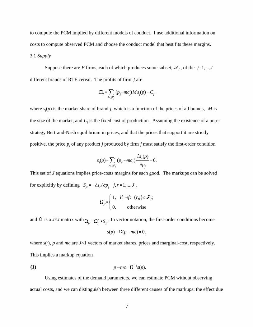
to compute the PCM implied by different models of conduct. I use additional information on

costs to compute observed PCM and choose the conduct model that best fits these margins.

3.1 Supply

Suppose there are F firms, each of which produces some subset, Þf , of the j=1,...,J

different brands of RTE cereal. The profits of firm f are

where sj(p) is the market share of brand j, which is a function of the prices of all brands, M is

the size of the market, and Cf is the fixed cost of production. Assuming the existence of a pure-

strategy Bertrand-Nash equilibrium in prices, and that the prices that support it are strictly

positive, the price pj of any product j produced by firm f must satisfy the first-order condition

This set of J equations implies price-costs margins for each good. The markups can be solved

for explicitly by defining , Sjr'&Msr /Mpj j, r'1,...,J

and is a J×J matrix with . In vector notation, the first-order conditions becomeS Sjr'S(

jr(Sjr

where s(·), p and mc are J×1 vectors of market shares, prices and marginal-cost, respectively.

This implies a markup equation

Using estimates of the demand parameters, we can estimate PCM without observing

actual costs, and we can distinguish between three different causes of the markups: the effect due

8

to the differentiation of the products, the portfolio effect, and the effect of price collusion. This

is done by evaluating the PCM in three hypothetical industry conduct models. The first structure

is that of single-product firms, in which the price of each brand is set by a profit-maximizing

agent that considers only the profits from that brand . The second is the current structure, where

multi-product firms set the prices of all their products jointly. The final structure is joint profit-

maximization of all the brands, which corresponds to monopoly or perfect price collusion. Each

of these is estimated by defining the ownership structure, Þf, and ownership matrix, S*.

PCM in the first structure arise only from product differentiation. The difference

between the margins in the first two cases is due to the portfolio effect. The last structure

bounds the increase in the margins due to price collusion. Once these margins are computed we

can choose between the models by comparing the predicted PCM to the observed PCM.

3.2 Demand

The exercise suggested in the previous section allows us to estimate the PCM and

separate them into different parts. However, it relies on the ability to consistently estimate the

own- and cross-price elasticities. As previously pointed out, this is not an easy task in an

industry with many closely related products. In the analysis below I follow the approach taken

by the discrete-choice literature and circumvent the dimensionality problem by projecting the

products onto a characteristics space, thereby making the relevant dimension the dimension of

this space and not the number of products.

Suppose we observe t=1,...,T markets, each with i=1,...,It consumers. In the estimation

below a market will be defined as a city-quarter combination. The conditional indirect utility of

consumer i from product j at market t is

9This specification assumes that the unobserved components are common to all consumers. Analternative is to model the distribution of the valuation of the unobserved characteristics, as in Das, Olley andPakes (1994). For a further discussion see Nevo (1998a).

9

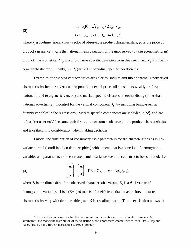
uijt'xj$(

i &"(

i pjt%>j%)>jt%,ijt,

i'1,...,It, j'1,...,Jt, t'1,...,T,(2)

"(

i

$(

i

'

"i

$i

%ADi%Evi , vi~ N(0, IK%1),(3)

where xj is K-dimensional (row) vector of observable product characteristics, pjt is the price of

product j in market t, >j is the national mean valuation of the unobserved (by the econometrician)

product characteristics, )>jt is a city-quarter specific deviation from this mean, and gijt is a mean-

zero stochastic term. Finally, are K+1 individual-specific coefficients.("(i $(

i )

Examples of observed characteristics are calories, sodium and fiber content. Unobserved

characteristics include a vertical component (at equal prices all consumers weakly prefer a

national brand to a generic version) and market-specific effects of merchandising (other than

national advertising). I control for the vertical component, >j, by including brand-specific

dummy variables in the regressions. Market-specific components are included in )>jt and are

left as "error terms".9 I assume both firms and consumers observe all the product characteristics

and take them into consideration when making decisions.

I model the distribution of consumers’ taste parameters for the characteristics as multi-

variate normal (conditional on demographics) with a mean that is a function of demographic

variables and parameters to be estimated, and a variance-covariance matrix to be estimated. Let

where K is the dimension of the observed characteristics vector, Di is a d×1 vector of

demographic variables, A is a (K+1)×d matrix of coefficients that measure how the taste

characteristics vary with demographics, and E is a scaling matrix. This specification allows the

10The distinction between "observed" and "unobserved" individual characteristics refers to auxiliary datasets and not to the main data source, which includes only aggregate quantities and average prices. Thedistribution of the "observed" characteristics can be estimated from these additional sources.

11The reasons for names will become apparent below.

10

ui0t'>0%B0Di%F0vi0%,i0t .

uijt'*jt(xj , pjt ,>j ,)>jt ;21)%µijt(xj ,pjt ,vi ,Di ;22)%,ijt

*jt' xj$&"pjt%>j%)>jt, µijt' [pjt,xj])((ADi%Evi)

(4)

individual characteristics to consist of demographics that are "observed" and additional

characteristics that are "unobserved", denoted Di and vi respectively.10

The specification of the demand system is completed with the introduction of an "outside

good"; the consumers may decide not to purchase any of the brands. Without this allowance a

homogenous price increase (relative to other sectors) of all products does not change quantities

purchased. The indirect utility from this outside option is

The mean utility of the outside good is not identified (without either making more assumptions

or normalizing one of the "inside" goods), thus I normalize >0 to zero. The coefficients, B0 and

F0, are not identified separately from an intercept, in equation (2), that varies with consumer

characteristics.

Let 2 = (21, 22) be a vector containing all parameters of the model. The vector 21=(",$)

contains the linear parameters and the vector 22=(vec(A), vec(E)) the non-linear parameters.11

Combining equations (2) and (3)

where is a (K+1)×1 vector. The utility is now expressed as the mean utility, represented[pjt, xj]

by *jt, and a mean-zero heteroskedastic deviation from that mean, µijt + gijt, which captures the

effects of the random coefficients.

12A comment is in place about the realism of the assumption that consumers choose no more than onebrand. Many households buy more than one brand of cereal in each supermarket trip but most people consumeonly one brand of cereal at a time, which is the relevant fact for this modeling assumption. Nevertheless, if one isstill unwilling to accept that this is a negligible phenomenon then this model can be viewed as an approximation tothe true choice model. An alternative is to explicitly model the choice of multiple products, or continuousquantities (as in Dubin and McFadden, 1984; or Hendel, 1998).

11

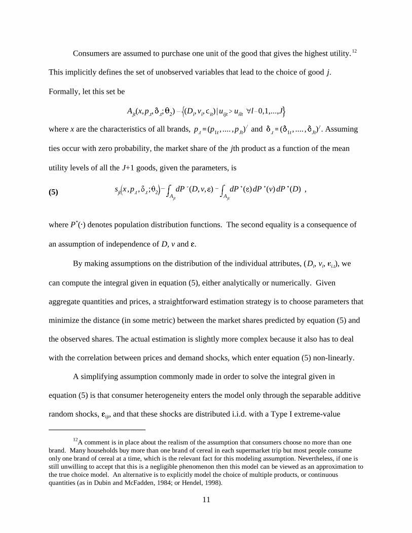
Ajt(x,p.t,*.t;22)' (Di, vi,,it) |uijt$uilt él'0,1,...,J

sjt x ,p.t , .t ; 2 'mAjt

dP ((D, v, )'mAjt

dP (( )dP ((v) dP ((D) ,(5)

Consumers are assumed to purchase one unit of the good that gives the highest utility.12

This implicitly defines the set of unobserved variables that lead to the choice of good j.

Formally, let this set be

where x are the characteristics of all brands, . Assumingp.t' (p1t , .... ,pJt)) and *.t' (*1t , .... ,*Jt)

)

ties occur with zero probability, the market share of the jth product as a function of the mean

utility levels of all the J+1 goods, given the parameters, is

where P*(@) denotes population distribution functions. The second equality is a consequence of

an assumption of independence of D, v and g.

By making assumptions on the distribution of the individual attributes, (Di, vi, gi.t), we

can compute the integral given in equation (5), either analytically or numerically. Given

aggregate quantities and prices, a straightforward estimation strategy is to choose parameters that

minimize the distance (in some metric) between the market shares predicted by equation (5) and

the observed shares. The actual estimation is slightly more complex because it also has to deal

with the correlation between prices and demand shocks, which enter equation (5) non-linearly.

A simplifying assumption commonly made in order to solve the integral given in

equation (5) is that consumer heterogeneity enters the model only through the separable additive

random shocks, gijt, and that these shocks are distributed i.i.d. with a Type I extreme-value

12

distribution. This assumption reduces the model to the well-known (multinomial) Logit model,

which is appealing due to its tractability though it restricts the own- and cross-price elasticities

(for details see McFadden, 1981; or BLP). Slightly less restrictive models, in which the i.i.d.

assumption is replaced with a variance components structure, are available (see the Generalized

Extreme Value model introduced by McFadden, 1978). The Nested Logit model and the

Principles of Differentiation Generalized Extreme Value model (see Bresnahan, Stern and

Trajtenberg, 1997) fall within this class. While less restrictive than the Logit model both models

derive substitution patterns from a priori segmentation.

The full model nests all of these other models and has several advantages over them.

First, it allows for flexible own-price elasticities, which will be driven by the different price

sensitivity of different consumers who purchase the various products, not by functional-form

assumptions about how price enters the indirect utility. Second, since the composite random

shock, µijt + gijt, is no longer independent of the product characteristics, the cross-price

substitution patterns will be driven by these characteristics. Such substitution patterns are not

constrained by a priori segmentation of the market, yet at the same time can take advantage of

this segmentation. Furthermore, McFadden and Train (1997) show that the full model can

approximate arbitrarily close any choice model. In particular, the multinomial Probit model (see

Hausman and Wise, 1978) and the "universal" Logit (see McFadden, 1981).

4. DATA AND ESTIMATION

4.1 The Data

The data required to consistently estimate the model previously described consists of the

following variables: market shares and prices in each market (in this paper a city-quarter), brand

characteristics, advertising and information on the distribution of demographics.

13I am grateful to Ronald Cotterill, the director of the Food Marketing Center at the University ofConnecticut, for making these data available.

13

Market shares and prices were obtained from the IRI Infoscan Data Base at the

University of Connecticut.13 Definition of the variables and the details of the data construction

are given in Appendix A. These data are aggregated by brand (for example different size boxes

are considered one brand), city and quarter. The data covers up to 65 different cities (the exact

number increases over time), and ranges from the first quarter of 1988 to the last quarter of

1992. The results presented below were computed using the 25 brands with the highest national

market shares in the last quarter of 1992. For all, except one, there are 1124 observations (i.e.,

they are present in all quarters and all cities). The exception is Post Honey Bunches of Oats,

which appears in the data only in the first quarter of 1989. The combined city-level market

share of the brands in the sample varies between 43 and 62 percent of the total volume of cereal

sold in each city and quarter. Combined national market shares vary between 55 and 60 percent.

I discuss below the potential bias from restricting attention to this set of products.

Summary statistics for the main variables are provided in Table 5. The last three

columns show the percentage of variance due to brand, city, and quarter dummy variables.

Controlling for the variation between brands, most of the variation in market shares, and even

more so in prices, is due to differences across cities. The variation in prices is due to both

exogenous and endogenous sources (i.e., variation correlated with demand shocks). Consistent

estimation will have to separate these effects. The Infoscan price and quantity data were

matched with a information on product characteristics and the distribution of individual

demographics obtained from the CPS, see Appendix A for details.

4.2 Estimation

I estimate the parameters of the models described in Section 3 using the data described in

14

pjt'mcjt% f(>jt,...)' (mcj% fj)% ()mcjt%)fjt) .(6)

the previous section by following Berry (1994) and BLP. The key point of the estimation is to

exploit a population moment condition that is a product of instrumental variables and a

(structural) error term, to form a (non-linear) GMM estimator. The error term is defined as the

unobserved product characteristics, (or just if brand dummy variables are included). >j%)>jt )>jt

The main technical difficulties in the estimation are the computation of the integral defining the

market shares, given in equation (5), and the inversion of the market share equations to obtain

the error term (which can be plugged into the objective function). Some details of the estimation

are given in Appendix A (for more details see BLP or Nevo, 1998a).

Besides slight differences in the implementation, the algorithm is similar to that used by

BLP with three notable exceptions. First, the instrumental variables and the identifying

assumptions that support them are different. A somewhat related point, I am able to identify the

demand side without specifying a functional form for the supply side, while BLP’s identification

relies on the functional form of a supply equation. Finally, due to the richness of the data I am

able to control for unobserved product characteristics by using brand fixed effects. In the next

two sections I detail the main differences with BLP.

4.3 Instruments

The key identifying assumption in the estimation is the population moment condition,

detailed in Appendix A, which requires a set of exogenous instrumental variables. In order to

understand the need for this assumption, and to understand why (non-linear) least squares

estimation will be inconsistent, we examine the pricing decision. By equation (1), prices are a

function of marginal costs and a markup term,

This can be decomposed into an overall mean and a deviation from this mean that varies by city

14See for example Bresnahan (1981, 1987), Berry (1994), BLP (1995), or Bresnahan, Stern andTrajtenberg (1997).

15It will not be exactly singular because one of the products was not present in all quarters.

15

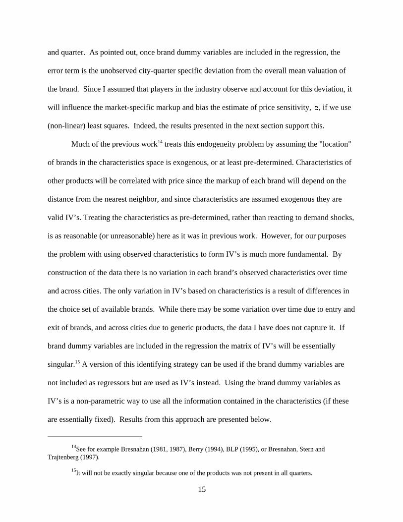
and quarter. As pointed out, once brand dummy variables are included in the regression, the

error term is the unobserved city-quarter specific deviation from the overall mean valuation of

the brand. Since I assumed that players in the industry observe and account for this deviation, it

will influence the market-specific markup and bias the estimate of price sensitivity, ", if we use

(non-linear) least squares. Indeed, the results presented in the next section support this.

Much of the previous work14 treats this endogeneity problem by assuming the "location"

of brands in the characteristics space is exogenous, or at least pre-determined. Characteristics of

other products will be correlated with price since the markup of each brand will depend on the

distance from the nearest neighbor, and since characteristics are assumed exogenous they are

valid IV’s. Treating the characteristics as pre-determined, rather than reacting to demand shocks,

is as reasonable (or unreasonable) here as it was in previous work. However, for our purposes

the problem with using observed characteristics to form IV’s is much more fundamental. By

construction of the data there is no variation in each brand’s observed characteristics over time

and across cities. The only variation in IV’s based on characteristics is a result of differences in

the choice set of available brands. While there may be some variation over time due to entry and

exit of brands, and across cities due to generic products, the data I have does not capture it. If

brand dummy variables are included in the regression the matrix of IV’s will be essentially

singular.15 A version of this identifying strategy can be used if the brand dummy variables are

not included as regressors but are used as IV’s instead. Using the brand dummy variables as

IV’s is a non-parametric way to use all the information contained in the characteristics (if these

are essentially fixed). Results from this approach are presented below.

16There is no claim made here with regards to the "optimality" of these IV’s. A potentially interestingquestion might be are there other ways of weighting the information from different cities.

16

Since this most-commonly-used approach will not work if brand fixed effects are

included I use two alternative sets of instrumental variables in an attempt to separate the

exogenous variation in prices (due to differences in marginal costs) and endogenous variation

(due to differences in unobserved valuation). First, I use an approach similar to that used by

Hausman (1996) and exploit the panel structure of the data. The identifying assumption is that,

controlling for brand-specific means and demographics, city-specific valuations are independent

across cities (but are allowed to be correlated within a city). Given this assumption, the prices of

the brand in other cities are valid IV’s. From equation (6) we see that prices of brand j in two

cities will be correlated due to the common marginal cost, but due to the independence

assumption will be uncorrelated with market-specific valuation. One could potentially use prices

in all other cities and all quarters as instruments. I use regional quarterly average prices

(excluding the city being instrumented) in all twenty quarters.16

There are several plausible situations in which the independence assumption will not

hold. Suppose there is a national (or regional) demand shock. For example, the discovery that

fiber reduces the risk of cancer. This discovery will increase the unobserved valuation of all

fiber- intensive brands in all cities, and the independence assumption will be violated. However,

the results below concentrate on well-established brands for which it seems reasonable to assume

there are less systematic demand shocks. Also, aggregate shocks to the cereal market will be

captured by time dummy variables.

Suppose one believes that local advertising and promotions are coordinated across city

borders, but are limited to regions, and that these activities influence demand. Then the

independence assumption will be violated for cities in the same region, and prices in cities in the

17

same region will not be valid instrumental variables. However, given the size of the IRI "cities"

(which in most cases are larger than MSA’s) and the size of the Census regions, this might be

less of a problem. The size of the IRI city determines how far the activity has to go in order to

cross city borders; the larger the city, the smaller the chance of correlation with neighboring

cities. Similarly, the larger the Census region the less likely is correlation with all cities in the

region. Finally, the IRI data is used by the firms in the industry, thus it is not unlikely that they

base their strategies on a city-level geographic split.

Determining how plausible are these, and possibly other situations is an empirical issue.

I approach it by examining another set of instrumental variables that attempts to proxy for the

marginal costs directly and compare the difference between the estimates implied by the

different sets of IV’s. The marginal costs include production (materials, labor and energy),

packaging, and distribution costs. Direct production and packaging costs exhibit little variation

and are too small a percentage of marginal costs to be correlated with prices. Also, except for

small variations over time, a brand dummy variable, which is included as one of the regressors,

proxies for these costs. The last component of marginal costs, distribution costs, includes the

cost of transportation, shelf space, and labor. These are proxied by region dummy variables,

which pick up transportation costs; city density, which is a proxy for the difference in the cost of

space; and average city earning in the supermarket sector computed from the CPS Monthly

Earning Files.

A persistent regional shock for certain brands will violate the assumption underlying the

validity of these IV’s. If, for example, all western states value natural cereals more than east-

coast states, region-specific dummy variables will be correlated with the error term. However,

in order for this argument to work the difference in valuation of brands has to be above and

18

beyond what is explained by demographics and heterogeneity since both are controlled for.

4.4 Brand-Specific Dummy Variables

As previously pointed out, one of the main differences between this paper and previous

work is the inclusion of brand-specific dummy variables as product characteristics. There are at

least two good reasons to include these dummy variables. First, in any case where we are unsure

that the observed characteristics capture the true factors that determine utility fixed effects

should be included in order to improve the fit of the model. Note that this helps fit the mean

utility level, *j(@), while substitution patterns are still driven by observed characteristics (either

physical characteristics or market segmentation), as is the case if we were not to include brand

fixed effects.

Furthermore, a major motivation (see Berry, 1994) for the estimation scheme previously

described is the need to instrument for the correlation between prices and the unobserved quality

of the product, >j. A brand-specific dummy variable captures the characteristics that do not vary

by market, namely, . Therefore, the correlation between prices and the unobservedxj$%>j

quality is fully accounted for and does not require an instrument. In order to introduce brand-

specific dummy variable we require observations on more than one market. However, even

without these dummy variables, fitting the model using observations from a single market is

difficult (see BLP, footnote 30).

There are two potential objections to the use of brand dummy variables. First, the main

motivation for the use of discrete-choice models was to reduce the dimensionality problem.

Introducing of brand fixed effects increases the number of parameters only with J (the number

of brands) and not J2 . Thus we have not defeated the purpose of using a discrete-choice model.

Furthermore, the brand dummy variables all enter as part of the linear parameters and do not

17This is the assumption required to justify the use of observed characteristics as IV’s. Here, unlikeprevious work, this assumption is used only to recover the taste parameters and does not impact the estimates ofprice sensitivity.

19

d'X$%> .

$$' (X )V &1d X)&1X )V &1

d$d, $>' $d&X $$

increase the computational difficulty.

In order to retrieve the taste coefficients, $, when brand fixed effects are included in the

regression, I use a minimum-distance procedure (as in Chamberlain, 1982). Let d denote the

J×1 vector of brand dummy coefficients, X be the J×K (K<J) matrix of product characteristics,

and > be the J×1 vector of unobserved product qualities. Then from (2)

If we assume that 17 the estimates of $ and > areE [> |X]'0,

where is the vector of coefficients estimated from the procedure described in the previous$d

section, and Vd is the variance-covariance matrix of these estimates. The coefficients on the

brand dummy variables provide an "unrestricted" estimate of mean utility. The minimum-

distance estimator projects these estimates onto a lower K-dimensional space, which is implied

by a "restricted" model that sets > to zero. Chamberlain provides a chi-squared test to evaluate

these restrictions.

5. RESULTS

5.1 Logit Results

As pointed out in Section 3, the Logit model yields restrictive and unrealistic substitution

patterns, and therefore is inadequate for measuring market power. Nevertheless, due to its

computational simplicity it is a useful tool in getting a feel for the data. In this section I use the

Logit model to examine: (1) the importance of instrumenting for price; and (2) the effects of the

different sets of instrumental variables discussed in the previous section.

18The unreported coefficients on the product characteristics are (s.e.): constant, -4.44 (0.04), fatcal, 0.17(0.04), sugar,2.7(0.09), mushy, -0.12 (0.011), fiber, 0.04 (0.06), all family segment, 0.53 (0.02), kids segment,0.47 (0.02), health segment, 0.53 (0.02).

19The results are essentially the same if I use only the regional average price for that quarter.

20

Table 5 displays the results obtained by regressing ln(Sjt) - ln(S0t) on prices, advertising

expenditures, brand and time dummy variables. In columns (i)-(iii) I report the results of

ordinary least squares regressions. The regression in column (i) includes observed product

characteristics, but not brand fixed effects, and therefore the error term includes the unobserved

product characteristic, >j.18 The regressions in columns (ii) and (iii) include brand dummy

variables and therefore fully control for >j. The effects of including brand-specific dummy

variables on the price and advertising coefficients are significant both statistically and

economically. However, even the coefficient on price given in column (iii) is relatively low.

The Logit demand structure does not impose a constant elasticity, and therefore the estimates

imply a different elasticity for each brand-city-quarter combination. The mean of the

distribution of own-price elasticities across the 27,862 observations is -1.53 (the median is -1.50)

with a standard deviation of 0.39, and 5.5% of the observations are predicted to have inelastic

demand.

Columns (iv)-(x) of Table 5 uses various sets of instrumental variables in two-stage least

squares regressions. The first set of results, presented in column (iv), is based on the same

specification as column (i) but uses brand dummy variables as IV’s. This is similar to the

identification assumptions used by much of the previous work (see Section 4.3). Indeed,

compared to column (i) the price coefficient has nearly doubled, but it is almost identical to the

coefficients from the OLS regression which includes brand dummy variables as regressors.

Column (v) uses the average regional prices in all twenty quarters19 as instrumental

20Furthermore, by adding city fixed effects to the regression we demonstrate that we have enoughvariation in the time dimension to identify the parameters, and the results are not driven purely by cross-sectional

21

variables in a two-stage least squares regression. Not surprisingly, the coefficient on price

increases and the estimated demand curves for all brand-city-quarter combinations are elastic

(the mean of the distribution is -3.38, the median is -3.30 and the standard deviation 0.85).

Column (vi) uses a different set of IV’s: the proxies for city level marginal costs. The

coefficient on price is similar in the two regressions.

The similarity between the estimates of the price coefficient continues to hold when we

introduce demographics into the regression. Columns (vii)-(viii) present the results from the

previous two sets of IV’s, while column (vi) presents an estimation using both sets of

instruments jointly. The addition of demographics increases the absolute value of the price

coefficient, leading to an increase in the absolute value of the price elasticity. As we recall from

the previous section, if there are regional demand shocks then both sets of IV’s are not valid.

City-specific valuations may be a function of demographics, and if demographics are correlated

within a region these valuations will be correlated. Under this story, adding demographics

eliminates the omitted-variable bias and improves the over-identification test statistic. The

coefficients on demographics capture the change in the value of the cereal relative to the outside

option as a function of demographics. The results suggest that the value of cereals increases

with income, while age and household size are non-significant. Demographics could potentially

be added to the regression in a more complex manner (for example, allowing for interactions

with the product characteristics), but since the purpose of the Logit model is mainly descriptive,

this is done only in the full model. Finally, column (x) allows for city-specific intercepts, which

control even further for city-level demand shocks. The results in this column are again almost

identical to the previous results.20

differences.

21It is well known that with a large enough sample a P2 test will reject essentially any model.

22In the previous sections I have focused my attention to the endogeneity of prices but little was saidabout the endogeneity of advertising. Conventional wisdom of this industry and these results might cast doubt onthis decision. I wish to point out several things. First, advertising varies by brand-quarter, and not by city, thus,potentially is less correlated with the errors. Second, I do not use the advertising coefficient in the analysis below;therefore, as long as bias, if it exists, in this coefficient does not impact the price elasticities there is no effect onthe conclusions reached below. Once I add brand fixed effects the IV’s used to instrument for price seem to haveno effect on the advertising coefficient, suggesting that the opposite might also be true (i.e., that instrumenting foradvertising would have little, or no, impact on estimates of price sensitivity).

22

The first stage R-squared and F-statistic for all the instrumental variable regressions are

high, suggesting (although not promising) that the IV’s have some power. The first-stage

regressions are presented in Appendix B. With the exception of the last column, the tests of

over-identification are rejected, suggesting that the identifying assumptions are not valid.

However, it is unclear whether the large number of observations is the reason for the rejection21

or that the IV’s are not valid.

The regressions also include advertising, which has a statistically significant coefficient.

With the exception of column (i) the estimated effect of advertising is roughly the same in all

specifications. The large coefficient in column (i) is a result of the correlation between

unobserved characteristics and advertising: brands with larger market shares tend to have higher

>j’s and also advertise more. Once we control for this potential endogeneity22 the mean elasticity

with respect to advertising is approximately 0.06, which seems low. A Dorfman-Steiner

condition requires advertising elasticities to be an order of magnitude higher. This is probably a

result of measurement error in advertising data. Non-linear effects in advertising were also

tested and were found to be insignificant.

The price-cost margins implied by the estimates are given in the first column of Table 8.

A discussion of these results is deferred to later. The important thing to take from these results is

23I sampled 40 individuals for each year, in total 200 for each city.

23

the similarity between estimates using the two sets of IV’s, and the importance of controlling for

demographics and heterogeneity. The similarity between the coefficients does not promise the

two sets of IV’s will produce identical coefficients in different models or that these are valid

IV’s. However, I believe that with proper control for demographics and heterogeneity, as in the

full model, these are valid IV’s.

5.2 Results from the Full Model

The estimates of the full model are based on equation (4) and were computed using the

procedure described in Appendix A. Predicted market shares are computed using equation (5)

and are based on the empirical distribution of demographics (as sampled from the March CPS),23

independent normal distributions (for v), and Type I extreme value (for g). The IV’s include

both average regional prices in all quarters and the cost proxies discussed in the previous section.

The results from the preferred specification are presented in Table 6. Additional specifications

are discussed and presented in Appendix B.

The means of the distribution of marginal utilities, $’s, are estimated by a minimum-

distance procedure described above and presented in the first column. All coefficients are

statistically significant and basically of the expected sign. The ability of the observed

characteristics to fit the coefficients of the brand dummy variables is measured by using the P2

test, described in Section 4.4, which is presented at the bottom of Table 6. Since the brand

dummy variables are estimated very precisely (due to the large number of observations) it is not

surprising that the restricted model is rejected.

Estimates of heterogeneity around these means are presented in the next few columns.

With the exception of the kids-segment dummy variable, Kids, taste parameters standard

24

deviations estimates are insignificant at conventional significance levels, while most interactions

with demographics are significant. The interpretation of the estimates is straight forward. For

example, the marginal valuation of sogginess increases with age and income. In other words,

adults are less sensitive to the crispness of a cereal as are wealthier consumers. The distribution

of the MUSHY coefficient can be seen in Figure 1; most of the consumers value sogginess in a

negative way, but approximately 15% of consumers actually prefer a mushy cereal.

The mean price coefficient is of the same order of magnitude as those presented in Table

5. However, the implied elasticities and margins are different, as discussed below. Coefficients

on the interaction of price with demographics are statistically significant. The estimate of the

standard deviation is not statistically significant, suggesting that most of the heterogeneity is

explained by the demographics (an issue we shall return to below). Older and above-average

income consumers tend to be less price sensitive. The distribution of the individual price

sensitivity can be seen in Figure 2. It does not seem to be normal, which is a result of the

empirical distribution of demographics. In principal, the tail of the distribution can reach

positive values % implying that the higher the price the higher the utility. For the given

specification the percent of positive price coefficients, given in the last row of the table, is only

0.7%. This is due to flexible interactions with demographics (specifications that don’t allow

these interactions are presented in Nevo, 1997a, there as much as 13% of the price coefficients

are positive.)

As noted above, all the estimates of the standard deviations are statistically insignificant,

suggesting that the heterogeneity in the coefficients is mostly explained by the included

demographics. A measure of the relative importance of the demographics and random shocks

can be obtained from the ratios of the variance explained by the demographics to the total

24Rossi, McCulloch, and Allenby (1996) find that using previous purchasing history helps explainheterogeneity above and beyond what is explained by demographics alone. Berry, Levinsohn and Pakes (1998)reach a similar conclusion using second choice data. The results of this paper do not suggest that previouspurchases or second-choices would have no value, they only suggest that the data rejects the assumed normaldistribution. This result is not driven by the aggregate data and would probably continue to hold for a number ofother parametric distributions (see the results of Kiser, 1996).

25

variation in the distribution of the estimated coefficients; these are over 90%. 24 Appendix B

presents the results of a specification that sets the random shocks, vi, to zero.

Table 7 presents a sample of estimated own- and cross-price elasticities. Each entry i, j,

where i indexes row and j column, gives the elasticity of brand i with respect to a change in the

price of j. Since the model does not imply a constant elasticity, this matrix will be different

depending on what values of the variables are used to evaluate it. Rather than choosing a

particular value (say the average, or a value at a particular market), I present the median of each

entry over the 1124 markets in the sample. The results are intuitive. For example, Lucky

Charms, a kids cereal, is most sensitive to a change in the price of Corn Pops and Froot Loops,

also kids cereals. At the same time it is least sensitive to a change in the price of cereals like

Corn Flakes, Total or Wheaties, all cereals aimed at different market segments. These

substitution patterns are persistent across the table.

An additional diagnostic of how far the results are from the restrictive form imposed by

the Logit model is given by examining the variation in the cross-price elasticities in each

column. As discussed in Section 2, the Logit restricts all elasticities within a column to be equal.

Therefore, an indicator of how well the model has overcome these restrictions is to examine the

variation in the estimated elasticities. One such measure is given by examining the ratio of the

maximum to the minimum cross-price elasticity (the Logit model implies a ratio of one.) This

ratio varies from 21 (Corn Flakes) to 3.5 (Shredded Wheat). Not only does this tell us the

results have overcome the Logit restrictions, but more importantly it suggests for which brands

25A formal specification test of the Logit model (in the spirit of Hausman and McFadden, 1984) is thetest of the hypothesis that all the non-linear parameters are jointly zero. This test is easily rejected.

26Comparing the absolute value of the elasticities across columns is somewhat meaningless, since in eachcolumn the absolute price change is different. In order to compare across columns semi-elasticities, or the percentchange in market share due to say a 10 cents change in price, need to be computed.

26

the characteristics do not seem strong enough to overcome the restrictions. This test therefore

suggests which characteristics we might want to add.25

Finally, the bottom row of Table 7 presents the elasticity of the share of the outside good

with respect to the price of the "inside" goods. By comparing the ratio of these elasticities to the

average in each column we see the relative importance of the outside good to each brand. For

example, the cross-price elasticity of the outside good is higher for Kellogg’s Corn Flakes than

Froot Loops. Not only is it higher in absolute terms, but it is higher as a ratio of the average

cross-price elasticity in that column.26 Once again this is an intuitive result. Private label

versions of Kellogg’s Corn Flakes are available and have higher shares than generic versions of

Froot Loops. All generic products are included in the outside good and therefore it should not

be surprising that the outside good is more sensitive to the price of Corn Flakes.

5.3 Additional Specifications and a Final Word About Endogeneity

The previous section presented in detail the preferred specification. Some additional

specifications are presented in Appendix B and more can be found in Nevo (1997a). Overall it

is important to note that even though these specifications are different in some aspects from the

preferred specification the conclusions described in the next section are robust. In addition to

the various specifications within the framework used here I also examined the multi-stage

demand system, which has recently been used by Hausman, Leonard and Zona (1994) and

Hausman (1996). Despite some interesting differences in the pattern of estimated cross-price

substitution, the conclusions reached in the next section are unchanged. A full presentation,

27

discussion and comparison of the results is beyond the scope of this paper (for details see Nevo,

1997a).

In addition to the work mentioned in the previous paragraph various other authors have

also studied the RTE cereal industry. Hausman (1996) explores the value of a new brand of

cereal by estimating a multi-level demand system using a weekly panel of brand-level sales and

prices in seven cities. His estimation exploits the time variation in the weekly prices to identify

the demand parameters. Thus despite the fact that I follow Hausman in using prices in other

cities as IV, our estimation strategies are somewhat different. From his results one can estimate

the effects computed in the next section. The conclusions are essentially identical. Kiser (1996)

and Shum (1998) use household-level rather than aggregate data to estimate demand for cereal.

Although these data might also yield inconsistent estimates, the reasons are different than here.

Therefore it is encouraging that the estimated own- and cross-price elasticities are very similar to

those produced here. All of these studies use different data sets and different identifying

assumptions than those used here. However, they all imply similar conclusions, which increases

the confidence in the results.

5.4 Price-Cost Margins

Predicted PCM

Given the demand parameters estimated in the previous sections, we can use equation (1)

to compute PCM for different conduct models. As explained in Section 3.1, I compute PCM for

three hypothetical industry structures, thus placing bounds on the importance of the different

causes for PCM. Table 8 presents the median PCM for the Logit and the full models using the

demand estimates of Tables 5 and 6. Different rows present the PCM that the three models of

pricing conduct predict. In principal each brand-city-quarter combination will have a different

27Medians rather than means are presented to eliminate the sensitivity to outliers. Computing the meansof the distribution with the 5% tails truncated yields essentially identical results.

28Accounting estimates of marginal costs and PCM are problematic (see for example Fisher andMcGowan, 1983). Here I use these estimates only as a crude measure of PCM and also I provide additionalinformation that bounds their magnitude.

28

predicted margin. The figures in the table are the median of these 27,862 numbers. 27

Although the mean price sensitivity estimated from the full model, given in Table 6, is

similar to the price coefficient estimated in the Logit model, given in Table 5, the implied

markups are different. Since the full model does a better job of estimating the cross-price

elasticities, it is not surprising that the difference increases as we go from single, to multi-

product firms, and then to joint ownership of the 25 brands used in the estimation. For the Logit

model we can use the estimates to compute the predicted PCM for brands that were not included

in the estimation. Essentially all we need is the price sensitivity, estimated from the sample, and

the market shares of additional brands. In the full model we need more information about the

additional products, not just their market share, and therefore cannot impute the PCM.

Observed PCM

In order to determine which model of conduct fits the industry, we need to compare the

PCM computed assuming different models of conduct to actual margins. For purpose of

comparing observed markups with those predicted by the theory above I have to distinguish

between manufacturers and retail margins. I do so by treating the retail margin as an additional

cost to producers. This assumption is consistent with a wide variety of models of manufacturers-

retailer interaction. Unfortunately, I do not observe actual margins and will have to use crude

accounting estimates.28 These estimates are given in Table 3. This estimate is taken from

Cotterill (1996) who is reporting from estimates given in a First Boston Report on the Kellogg

Company. Similar estimates can be found in Corts (1996a). The relative comparison for our

29

purposes is the gross retail margin, estimated at 46.0%. Note, that this margin does not include

promotional costs, some of which can be argued to be marginal costs (for example, coupon

rebates). For the conclusions below this makes my estimate a conservative one.

The accounting estimates are supported by Census data (presented in Table 2) which, as

we saw, are slightly higher because they are average variable costs and can therefore be

considered an upper bound to PCM. A lower bound on the margins is the margin between the

price of national brands and the corresponding private labels. Using data from Wongtrakool

(1994), these margins are approximately 31%. Prices of private labels will be higher than

marginal costs for several reasons. First, they also potentially include a markup term, but lower

than the national brands. Second, the private label manufacturers might have different marginal

costs, most likely higher. For these reasons this margin is only a lower bound on PCM.

Testing the Models

The accounting estimates of marginal costs and the implied margins are a crude estimate

for the "typical" brand. Nevertheless, the PCM predicted by the different models are different

enough that this crude measure can still be used to separate the different effects. Using the

confidence intervals provided in Table 8 we can reject the null hypothesis that either the

"typical" margins, presented in Table 3, or the bounds, discussed in the previous section, are

equal to those predicted by the model of joint profit maximization for the 25 brands.

Furthermore, we cannot reject the null hypothesis that these quantities are consistent with the

prediction of the multi-product Nash-Bertrand equilibrium.

One might wonder how restricting the analysis to the top 25 brands alters the results and

conclusion. In principal the estimates of price sensitivity should not be biased by this sample

selection, and indeed some analysis performed with different samples suggests this is the case.

30

Therefore, the only potential differences are in the margins computed in Table 8. As previously

noted, in order to compute the quantities given in the table for more brands in the full model,

these brands have to be part of the sample. Since this is somewhat infeasible I will argue that

the likely outcome of including more brands is to strengthen the conclusions. It is more

probable that the smaller brands, not included in the sample, have a higher, in absolute value,

own-price elasticity (relative to similar brands that are in the sample) and therefore the PCM

predicted by the first model will go down. This effect will be completely offset if, rather than

giving equal weight to all brands, we weight the observations by market shares (the market-

share-weighted mean equivalent of the results in Table 8 are roughly 2-3 percentage points

higher, which are the likely effect of including smaller brands). For the other two models there

is an additional effect. Including more products in the "inside" goods rather than the "outside"

good will tend to increase the predicted PCM. The more products included, the larger the effect,

which implies that the effect on the fully collusive model will be larger. An idea of the potential

increase can be seen by examining the Logit results. The effects for the full model are likely to

be even larger. This implies that the PCM predicted by the multi-product Nash-Bertrand model

are likely to be even closer to observed quantities, while the PCM predicted by the collusive

model will be even further. In this sense the results of Table 8 are conservative.

There are at least two alternative testing methods that have been previously used in

similar situations. First, a strategy that has been successfully used in homogenous-goods

industries is to define conduct parameters that measure the degree of competition (see

Bresnahan, 1989). In addition to the problems associated with how one should interpret these

parameters (see for example Corts, 1999), the identification requirements for this strategy are

unlikely to be met in differentiated-product industries (see Nevo 1998b). The second alternative

31

is to construct a formal test of non-nested hypotheses (for example, see Bresnahan, 1987; or

Gasmi, Laffont and Vuong, 1992). These methods require evaluating the likelihood of each

model, which can be derived only after making additional assumptions. In particular, I would

have to make assumptions on the distribution of the error terms and fully define a supply

equation. Not only are both non-trivial assumptions, but based on the data and the unrestricted

specification used here there seems to be no natural set of assumptions to make.

6. CONCLUSIONS AND EXTENSIONS

This paper used a random coefficients discrete choice (mixed Logit) model to estimate a

brand-level demand system for RTE cereal. Parameter identification exploited the panel

structure of the data, and was based on an independence assumption of demand shocks across

cities for each brand. The estimates were supported by different identifying assumptions. The

estimated elasticities were used to compute price cost margins that would prevail under different

conduct models. These different models were tested by comparing the predictions to crude

observed measures of margins. A Nash-Bertrand pricing game, played between multi-product

firms (as the firms in the industry are), was found to be consistent with observed price-cost

margins. Furthermore, it seems that if any significant price collusion existed, the observed

margins would have been much higher. If we are willing to accept Nash-Bertrand as a

benchmark of non-collusive pricing, we are left to conclude, unlike previous work, that even

with PCM greater than 45%, prices in the industry are not a result of collusive behavior.

The results rule out an extreme version of cooperative pricing, one in which all firms

jointly maximize profits. There is a continuum of models that were not tested here. For

example, the results in the this paper do not rule out cooperative pricing between a subset of

products (say Kellogg’s and Post Raisin Bran) or producers (say Post and Nabisco). The

32

methods and test used here could, in principal, deal with these additional models but would

require more detailed cost data.

Most economists are familiar with this industry from the research of Schmalensee

(1978), which lays out the economic argument at the foundation of the FTC’s "shared

monopoly" case against the industry in the 1970's. Even though the standard description of the

complaint will include a claim of cooperative pricing, the core of the case was brand

proliferation and its use as a barrier to entry, not cooperative pricing. As much as I would like

to claim that this paper proves or disproves the FTC’s case, I cannot do so. I find that the high

observed PCM are primarily due to the firms’ ability to maintain a portfolio of differentiated

brands and influence the perceived quality of these brands by means of advertising. In a sense

my analysis suggests that, whether right or wrong, the FTC’s claim focused on the important

dimensions of competition. In order to make claims regarding the anti-competitive effects of

brand introduction and advertising one would have to extend the model to deal with these

dimensions explicitly.

Understanding the form of price competition has at least two immediate uses. Structural

models of demand and supply have recently gained popularity for analysis of mergers. These

models rely on estimates of demand and assumptions about pre- and post-merger equilibrium to

predict the effects of a merger. Nevo (1997b) uses the model, data and results of this paper for

such an analysis. A different application of the results and methods of this paper is to welfare

analysis. For example, Hausman (1996) uses estimates of demand and assumptions about short-

run price competition to evaluate the welfare gains from introduction of new goods. The results

and conclusions of this paper can be used as arguments for or against the assumptions used in

such an analysis.

33

REFERENCES

Berry, S. (1994), “Estimating Discrete-Choice Models of Product Differentiation,” Rand Journal

of Economics, 25, 242-262.

Berry, S., J. Levinsohn, and A. Pakes (1995), “Automobile Prices in Market Equilibrium,”

Econometrica, 63, 841-890.

Berry, S., J. Levinsohn, and A. Pakes (1998), “Differentiated Products Demand Systems from a

Combination of Micro and Macro Data: The New Car Market,” NBER Working Paper

no. 6481.

Bresnahan, T. (1981), “Departures from Marginal-Cost Pricing in the American Automobile

Industry,” Journal of Econometrics, 17, 201-227.

Bresnahan, T. (1987), “Competition and Collusion in the American Automobile Oligopoly: The

1955 Price War,” Journal of Industrial Economics, 35, 457-482.

Bresnahan, T. (1989), “Empirical Methods for Industries with Market Power,” in R.

Schmalensee and R. Willig, eds., Handbook of Industrial Organization, Vol. II,

Amsterdam: North-Holland.

Bresnahan, T., S. Stern, and M. Trajtenberg (1997), “Market Segmentation and the Sources of

Rents from Innovation: Personal Computers in the Late 1980's,” RAND Journal of

Economics, 28.

Bruce, S., and B. Crawford (1995), Cerealizing America, Boston: Faber and Faber.

Cardell, N.S. (1989), Extensions of the Multinomial Logit: The Hedonic Demand Model, The

Non-Independent Logit Model, and the Ranked Logit Model, Ph.D. Dissertation, Harvard

University.

Chamberlain, G. (1982), “Multi Variate Regression Models for Panel Data,” Journal of

34

Econometrics, 18(1), 5-46.

Corts, K.S. (1996a), “The Ready-to-eat Breakfast Cereal Industry in 1994 (A),” Harvard

Business School case number N9-795-191.

Corts, K.S. (1999), “Conduct Parameters and the Measurement of Market Power,” Journal of

Econometrics, 88, 227-250.

Cotterill, R.W. (1996), “High Cereal Prices and the Prospects for Relief by Expansion of Private

Label and Antitrust Enforcement,” Testimony offered at the Congressional Forum on the

Performance of the Cereal Industry, Washington D.C., March 12.

Das, S., S. Olley, and A. Pakes (1994), “Evolution of Brand Qualities of Consumer Electronics in

the U.S.,” mimeo.

Dubin, J. and D. McFadden (1984), “An Econometric Analysis of Residential Electric Appliance

Holding and Consumption,” Econometrica, 52, 345-362.

Gasmi, F., J. J. Laffont and Q. Vuong (1992), “Econometric Analysis of Collusive Behavior in a

Soft-Drink Market,” Journal of Economics & Strategy, 1(2), 277-311.

Fisher, F. M. and J. J. McGowan (1983), “On the Misuse of Accounting Rates of Return to Infer

Monopoly Profits,” American Economic Review, 73, 82-97.

Fruhan, W.H. (1979), Financial Strategy: Studies in the Creation, Transfer, and Destruction of

Shareholder Value, Homewood, IL: Irwin.

Hausman, J. (1983), “Specification and Estimation of Simultaneous Equations Models,”in Z.

Griliches and M. Intiligator, eds., Handbook of Econometrics, Amsterdam: North

Holland.

Hausman, J. and D. McFadden (1984), “Specification Tests for the Multinomial Logit Model,”

Econometrica, 52(5), 1219-1240.

35

Hausman, J. (1996), “Valuation of New Goods Under Perfect and Imperfect Competition,”in T.

Bresnahan and R. Gordon, eds., The Economics of New Goods, Studies in Income and

Wealth Vol. 58, Chicago: National Bureau of Economic Research.

Hausman, J., G. Leonard, and J.D. Zona (1994), “Competitive Analysis with Differentiated

Products,” Annales D’Economie et de Statistique, 34, 159-80.

Hausman, J., and D. Wise (1978), “A Conditional Probit Model for Qualitative Choice: Discrete

Decisions Recognizing Interdependence and Heterogeneous Preferences,” Econometrica,

49, 403-26.

Hendel, I. (1998), “Estimating Multiple Discrete Choice Models: An Application to

Computerization Returns,” forthcoming Review of Economic Studies.

Kiser, E. K. (1996), “Heterogeneity in Price Sensitivity: Implications for Price Discrimination,”

mimeo, University of Wisconsin-Madison.

McFadden, D. (1973), “Conditional Logit Analysis of Qualitative Choice Behavior,” in P.

Zarembka, eds., Frontiers of Econometrics, New York, Academic Press.

McFadden, D. (1978), “Modeling the Choice of Residential Location,” in A. Karlgvist, et al.,

eds., Spatial Interaction Theory and Planning Models, Amsterdam: North-Holland.

McFadden, D. (1981), “Econometric Models of Probabilistic Choice,” in C. Manski and D.

McFadden, eds., Structural Analysis of Discrete Data, pp. 198-272, Cambridge: MIT

Press.

McFadden, D. and K. Train (1997), “Mixed MNL Models for Discrete Response,” University of

California at Berkeley, mimeo.

Mueller, D.C. (1986), Profits in the Long Run, Cambridge: Cambridge University Press.

Nevo, A. (1997a), Demand for Ready-to-Eat Cereal and Its Implications for Price Competition,

36

Merger Analysis, and Valuation of New Goods, Ph.D. Dissertation, Harvard University.

Nevo, A. (1997b), "Mergers with Differentiated Products: The Case of Ready-to-Eat Cereal,"

University of California at Berkeley, mimeo (available http://emlab.berkeley.edu/~nevo).

Nevo, A. (1998a), "A Research Assistant’s Guide to Random Coefficients Discrete Choice

Models of Demand,” NBER Technical Paper no. 221 (an updated version and computer

code available at http://emlab.berkeley.edu/~nevo).

Nevo, A. (1998b), “Identification of the Oligopoly Solution Concept in a Differentiated-Products

Industry,” Economics Letters, 59, 391-395.

Nevo, A. and C. Wolfram (1999), “Prices and Coupons for Breakfast Cereals,” NBER Working

Paper no. 6932.

Rossi, P., R.E. McCulloch, and G.M. Allenby (1996), “The Value of Purchase History Data in

Target Marketing,” Marketing Science, 15(4), 321-40.

Scherer, F., M. (1982), “The Breakfast Cereal Industry,” in W. Adams, ed., The Structure of

American Industry, New York: Macmillian.

Schmalensee, R. (1978), “Entry Deterrence in the Ready-to-Eat Breakfast Cereal Industry,” Bell

Journal of Economics, 9, 305-327.

Shum, M. (1998), “Does Advertising Substitute for Experience? Evidence from the Breakfast

Cereal Market,” University of Toronto, mimeo.

Wongtrakool, B. (1994), "An Assessment of the "Cereal Killers": Private Labels in the Ready-

to-eat Cereal Industry," Senior Thesis, Harvard University.

29This was done by using the serving weight suggested by the manufacturer, which are assumed correct(or at least proportional to the "true" serving weight).

30The sources include: magazines, Sunday magazines, newspapers, outdoor, network television, spottelevision, syndicated television, cable networks, network radio and national spot radio.

31I wish to thank Sandy Black for suggesting this variable and helping me classify the various brands.

37

APPENDIX A: DATA AND ESTIMATION DETAILS

Data

The data described in Section 4 were obtained from various sources. Quantity and pricedata were obtained from the Food Marketing Policy Center at the University of Connecticut.These data were collected by Information Resources, Inc. (IRI), a marketing firm in Chicago,using scanning devices in a national random sample of supermarkets located in various metropolitan areas and rural towns. Weekly data for UPC-coded products are drawn from asample which represents the universe of supermarkets with annual sales of more than $2 milliondollars, accounting for 82% of grocery sales in the US. In most cities the sample covers morethan 20% of the relevant population, and due to the importance of the sample to its customers,IRI makes an effort to make the sample representative. This is confirmed by unpublishedanalysis conducted by the BLS.

Market shares are defined by converting volume sales into number of servings sold,29 anddividing by the total potential number of servings in a city in a quarter. This potential wasassumed to be one serving per capita per day. The market share of the outside good was definedas the difference between one and the sum of the inside goods market shares. A price variablewas created by dividing the dollar sales by the number of servings sold, and was deflated using aregional urban consumers CPI. The dollar sales reflect the price paid by consumers at theregister, generating an average real per-serving transaction price. However, the sales data doesnot account for any manufacturers coupons.

Advertising data was taken from the Leading National Advertising data base, whichcontains quarterly national advertising expenditures by brand collected from 10 media sources.30 I used the total of the 10 types of media.

Product characteristics were collected in local supermarkets by examining cereal boxes. This implicitly assumes that the characteristics have not changed since 1988. Although this isnot exactly true, it seems a reasonable first approximation. Each cereal was classified into"mushy" or not, depending on its sogginess in milk.31

Information on the distribution of demographics was obtained by sampling individualsfrom the March Current Population Survey for each year. I sampled 50 draws for each city ineach year. Individual income was obtained by dividing household income by the size of thehousehold. The variable Child was defined as a dummy variable which equals one if age is lessthan sixteen. The national averages obtained here are representative of Census statistics. However, the statistics on city-level demographics do not exactly match the analogous statisticsfrom Census data. This is due to the small sample size, and will have to be accounted in theestimation as an additional source of variation.

Finally, instrumental variables were constructed using two additional data sources. An

32I.e., A=Z’Z, which is the "optimal" weight matrix under the assumption of homoscedasticity.

38

E Z )@T(2() '0 ,(A-1)

$2'argmin2

T(2))ZA &1 Z )T(2) ,(A-2)

s.t x,p.t ,*.t ;22 'S.t ,(A-3)

Tjt'*jt(x, p.t,S.t;22)& (xj$%"pjt) .(A-4)

average of wages paid in the supermarket sector in each city was constructed from the NBERCPS Monthly Earning Extracts. Estimates of city density were taken from the BLS, as wereregional price indices.

The brands used in the analysis are given in Table A1 and summary statistics for thevariables used are given in Table A2

EstimationLet Z =[z1,...,zM] be a set of instruments such that

where T, a function of the model parameters, is an error term defined below and 2* denotes thetrue value of these parameters. The GMM estimate is

where A is a consistent estimate of . Following Berry(1994), I define the error termE[Z )TT)Z]by solving for the mean utility levels, *.t, that solve the implicit system of equations

where is the market share function defined by equation (5), and are the observed markets.t(·) S.tshares. For the Logit model the solution, is equal to while for the*jt(x,p.t,S.t ;22), ln(Sjt)& ln(S0t),full model this inversion is done numerically. Once this inversion has been done, the error termis defined as

If we want to include brand, time or city variables they would also be included in the right handside. We can now see the reason for distinguishing between 21 and 22: 21 enters this term, andthe GMM objective function, in a linear fashion, while 22 enters non-linearly.

If brand fixed effects are not included the error term, as defined by equation (A-4), is theunobserved product characteristic, >j. However, due to the richness of my data I am able toinclude brand-specific dummy variables as product characteristics. These dummy variablesinclude both the mean quality index of observed characteristics, , and the unobserved$xjcharacteristics, >j. Thus, the error term is the city-quarter specific deviation from the meanvaluation, i.e., )>jt. The inclusion of brand dummy variables introduce a challenge in estimatingthe taste parameters, $, which was dealt with in Section 4.4.

In the Logit model, with the appropriate choice of a weight matrix,32 this proceduresimplifies to two-stage least squares regression of . In the full randoml n ( Sjt)& ln(S0t)coefficients model, both the computation of the market shares, and the "inversion" in order to get

, have to be done numerically. The value of the estimate in equation (A-2) is then*jt(@)computed using a non-linear search. This search is simplified in two ways. First, the first-orderconditions of the minimization problem defined in equation (A-2) with respect to 21 are linear inthese parameters. Therefore, these linear parameters can be solved for (as a function of the otherparameters) and plugged into the rest of the first-order conditions, limiting the non-linear searchto only the non-linear parameters. Second, the results in the paper were computed using a Quasi-

39

Newton method with a user supplied gradient. This was found to work much faster than theNelder-Mead non derivative simplex search method used by BLP. For details of thecomputation algorithm, including a MATLAB computer code, see Nevo (1998a).

APPENDIX B: ADDITIONAL REGRESSIONS

This Appendix presents some additional results. Table B1 presents the first stageregressions that generated the results presented in Table 5. The columns are labeled to matchthose of Table 5. Table B2 presents some additional specifications. The first column presentsthe estimates from the preferred specification setting the unobserved shocks, vi’s, to zero forsome of the characteristics. The estimates are essentially unchanged, as are the estimatedmargins, which are presented at the bottom of the table. This similarity continues to hold if I setthe unobserved shocks to zero for all characteristics; thus, supporting the claim made in the textthat the heterogeneity is driven by the demographics and not the random shocks.

Columns (ii)-(iv) are the full model version of columns (i), (iii) and (iv) of Table 5.Column (ii) and (iii) are NLLS estimates of the full model not including and including branddummy variables as characteristics, respectively. The specification in column (iv) does notinclude the brand dummies in the demand but uses them as IV. As explained in the text this forthese data it is the equivalent of using brand characteristics as IV’s. The mean of the pricesensitivity is almost identical to that presented in Table 5, but the estimates suggest a widedispersion around this mean, especially for the estimates that do not include the brand dummyvariables in the demand (see the large percentage of price coefficients greater than zero). Theresults in the last column are estimated very imprecisely, which is not surprising given that I didnot use any of the variance reducing methods employed by BLP.

I also examined specifications, equivalent to those presented in Table 5 column (x),which include city specific intercepts. The point estimates are close to those of the preferredspecification but the standard errors are very large, which is not surprising given thatdemographics are approximately constant during the sample period.

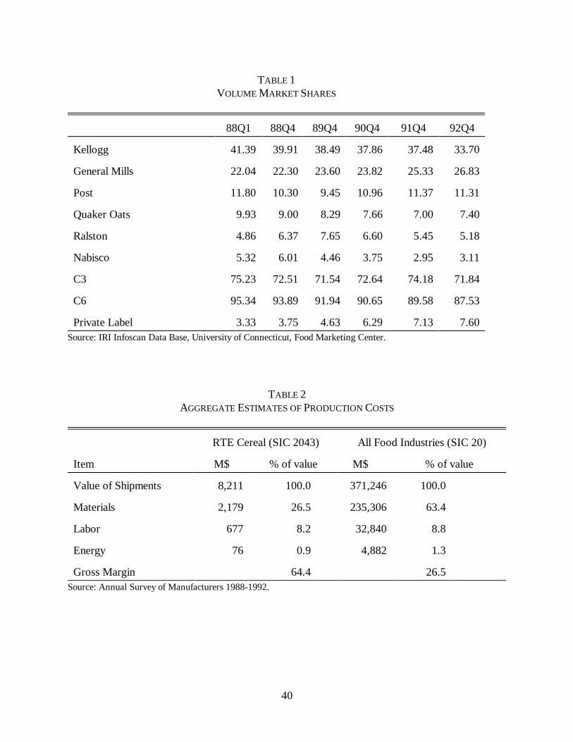
40

TABLE 1VOLUME MARKET SHARES

88Q1 88Q4 89Q4 90Q4 91Q4 92Q4

Kellogg 41.39 39.91 38.49 37.86 37.48 33.70

General Mills 22.04 22.30 23.60 23.82 25.33 26.83

Post 11.80 10.30 9.45 10.96 11.37 11.31

Quaker Oats 9.93 9.00 8.29 7.66 7.00 7.40

Ralston 4.86 6.37 7.65 6.60 5.45 5.18

Nabisco 5.32 6.01 4.46 3.75 2.95 3.11

C3 75.23 72.51 71.54 72.64 74.18 71.84

C6 95.34 93.89 91.94 90.65 89.58 87.53

Private Label 3.33 3.75 4.63 6.29 7.13 7.60Source: IRI Infoscan Data Base, University of Connecticut, Food Marketing Center.

TABLE 2AGGREGATE ESTIMATES OF PRODUCTION COSTS

RTE Cereal (SIC 2043) All Food Industries (SIC 20)

Item M$ % of value M$ % of value

Value of Shipments 8,211 100.0 371,246 100.0

Materials 2,179 26.5 235,306 63.4

Labor 677 8.2 32,840 8.8

Energy 76 0.9 4,882 1.3

Gross Margin 64.4 26.5Source: Annual Survey of Manufacturers 1988-1992.

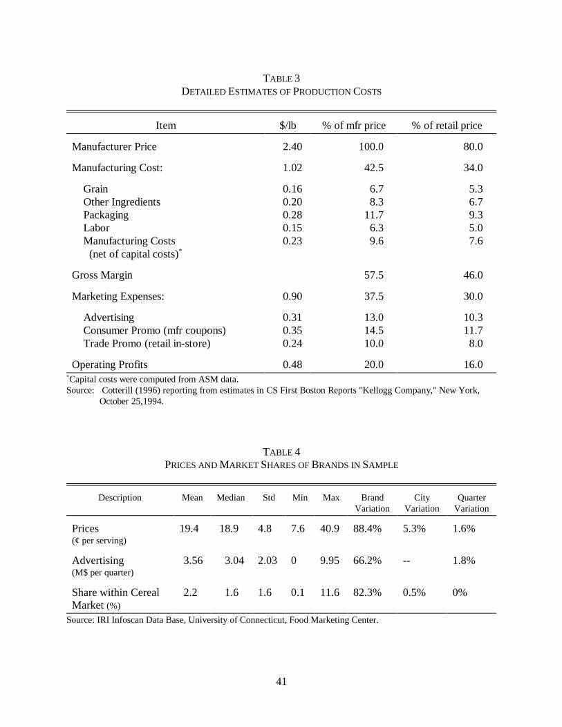
41

TABLE 3DETAILED ESTIMATES OF PRODUCTION COSTS

Item $/lb % of mfr price % of retail price

Manufacturer Price 2.40 100.0 80.0

Manufacturing Cost: 1.02 42.5 34.0

Grain Other Ingredients Packaging Labor Manufacturing Costs (net of capital costs)*

0.160.200.280.150.23

6.78.3

11.76.39.6

5.36.79.35.07.6

Gross Margin 57.5 46.0

Marketing Expenses: 0.90 37.5 30.0

Advertising Consumer Promo (mfr coupons) Trade Promo (retail in-store)

0.310.350.24

13.014.510.0

10.311.78.0

Operating Profits 0.48 20.0 16.0*Capital costs were computed from ASM data.Source: Cotterill (1996) reporting from estimates in CS First Boston Reports "Kellogg Company," New York,

October 25,1994.

TABLE 4PRICES AND MARKET SHARES OF BRANDS IN SAMPLE

Description Mean Median Std Min Max BrandVariation

CityVariation

QuarterVariation

Prices (¢ per serving)

19.4 18.9 4.8 7.6 40.9 88.4% 5.3% 1.6%

Advertising(M$ per quarter)

3.56 3.04 2.03 0 9.95 66.2% -- 1.8%

Share within CerealMarket (%)

2.2 1.6 1.6 0.1 11.6 82.3% 0.5% 0%

Source: IRI Infoscan Data Base, University of Connecticut, Food Marketing Center.

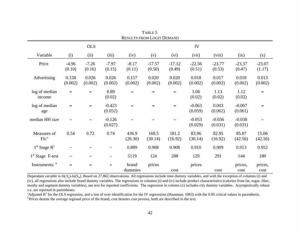
42

TABLE 5

RESULTS FROM LOGIT DEMAND

OLS IV

Variable (i) (ii) (iii) (iv) (v) (vi) (vii) (viii) (ix) (x)

Price -4.96(0.10)

-7.26(0.16)

-7.97(0.15)

-8.17(0.11)

-17.57(0.50)

-17.12(0.49)

-22.56(0.51)

-23.77(0.53)

-23.37(0.47)

-23.07(1.17)

Advertising 0.158(0.002)

0.026(0.002)

0.026(0.002)

0.157(0.002)

0.020(0.002)

0.020(0.002)

0.018(0.002)

0.017(0.002)

0.018(0.002)

0.013(0.002)

log of medianincome

% % 0.89(0.02)

% % % 1.06(0.02)

1.13(0.02)

1.12(0.02)

%

log of medianage

% % -0.423(0.052)

% % % -0.063(0.059)

0.003(0.062)

-0.007(0.061)

%

median HH size % % -0.126(0.027)

% % % -0.053(0.029)

-0.036(0.031)

-0.038(0.031)

%

Measures ofFit:a

0.54 0.72 0.74 436.9(26.30)

168.5(30.14)

181.2(16.92)

83.96(30.14)

82.95(16.92)

85.87(42.56)

15.06(42.56)

1st Stage R2% % % 0.889 0.908 0.908 0.910 0.909 0.913 0.952

1st Stage F-test % % % 5119 124 288 129 291 144 180

Instruments: b% % % brand

dummiesprices

costprices

costprices,

costprices,

costDependant variable is ln(Sjt)-ln(S0t). Based on 27,862 observations. All regressions include time dummy variables, and with the exception of columns (i) and(iv), all regressions also include brand dummy variables. The regressions in columns (i) and (iv) include product characteristics (calories from fat, sugar, fiber,mushy and segment dummy variables), see text for reported coefficients. The regression in column (x) includes city dummy variables. Asymptotically robusts.e. are reported in parentheses.aAdjusted R2 for the OLS regression, and a test of over identification for the IV regressions (Hausman, 1983) with the 0.95 critical values in parenthesis.b Prices denote the average regional price of the brand, cost denotes cost proxies, both are described in the text.

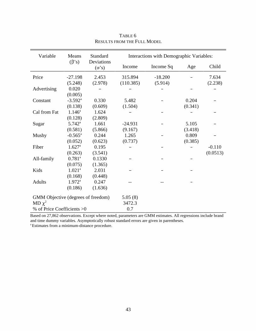
43

TABLE 6

RESULTS FROM THE FULL MODEL

Variable Means($’s)

Standard Deviations

(F’s)

Interactions with Demographic Variables:

Income Income Sq Age Child

Price

Advertising

Constant

Cal from Fat

Sugar

Mushy

Fiber

All-family

Kids

Adults

-27.198(5.248)0.020

(0.005)-3.592a

(0.138)1.146a

(0.128)5.742a

(0.581)-0.565a

(0.052)1.627a

(0.263)0.781a

(0.075)1.021a

(0.168)1.972a

(0.186)

2.453(2.978)

%

0.330(0.609)1.624

(2.809)1.661

(5.866)0.244

(0.623)0.195

(3.541)0.1330(1.365)2.031

(0.448)0.247

(1.636)

315.894(110.385)

%

5.482(1.504)

%

-24.931(9.167)1.265

(0.737)%

%

%

--

-18.200(5.914)

%

%

%

%

%

%

%

%

--

%

%

0.204(0.341)

%

5.105(3.418)0.809

(0.385)%

%

%

%

7.634(2.238)

%

%

%

%

%

-0.110(0.0513)

GMM Objective (degrees of freedom)MD P2

% of Price Coefficients >0

5.05 (8)3472.3

0.7Based on 27,862 observations. Except where noted, parameters are GMM estimates. All regressions include brandand time dummy variables. Asymptotically robust standard errors are given in parentheses.a Estimates from a minimum-distance procedure.

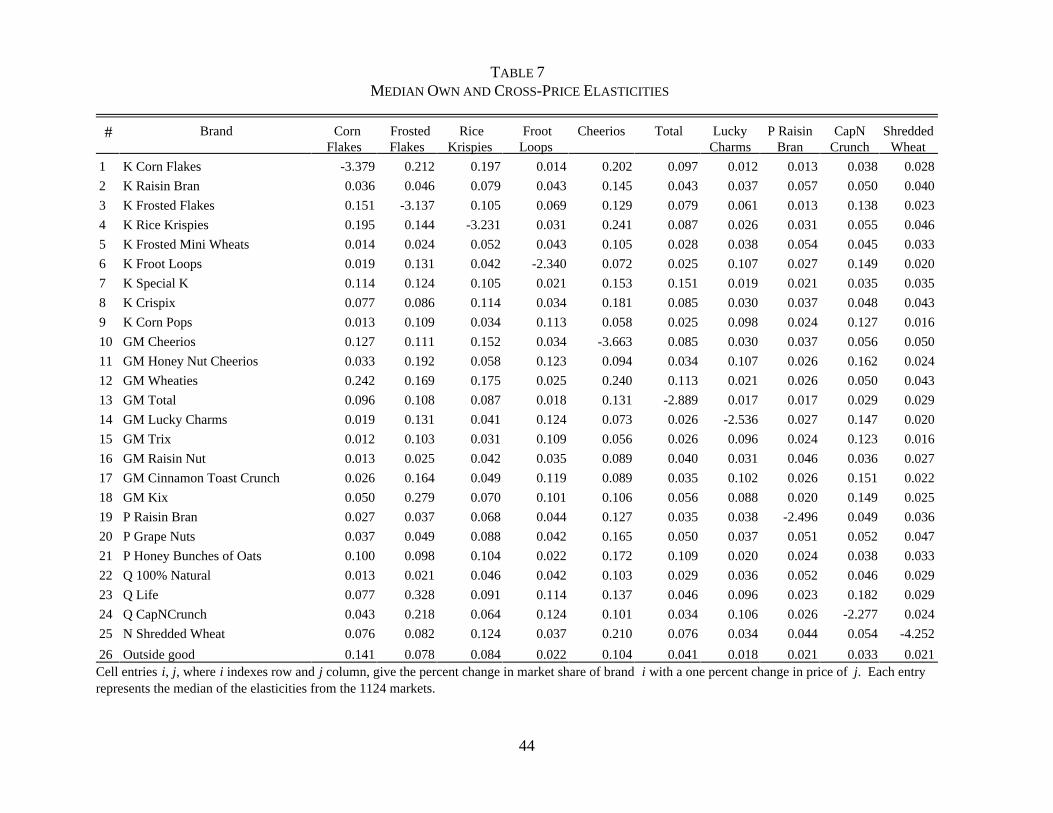
44

TABLE 7 MEDIAN OWN AND CROSS-PRICE ELASTICITIES

# Brand CornFlakes

FrostedFlakes

RiceKrispies

FrootLoops

Cheerios Total LuckyCharms

P RaisinBran

CapNCrunch

ShreddedWheat

1 K Corn Flakes -3.379 0.212 0.197 0.014 0.202 0.097 0.012 0.013 0.038 0.028

2 K Raisin Bran 0.036 0.046 0.079 0.043 0.145 0.043 0.037 0.057 0.050 0.040

3 K Frosted Flakes 0.151 -3.137 0.105 0.069 0.129 0.079 0.061 0.013 0.138 0.023

4 K Rice Krispies 0.195 0.144 -3.231 0.031 0.241 0.087 0.026 0.031 0.055 0.046

5 K Frosted Mini Wheats 0.014 0.024 0.052 0.043 0.105 0.028 0.038 0.054 0.045 0.033

6 K Froot Loops 0.019 0.131 0.042 -2.340 0.072 0.025 0.107 0.027 0.149 0.020

7 K Special K 0.114 0.124 0.105 0.021 0.153 0.151 0.019 0.021 0.035 0.035

8 K Crispix 0.077 0.086 0.114 0.034 0.181 0.085 0.030 0.037 0.048 0.043

9 K Corn Pops 0.013 0.109 0.034 0.113 0.058 0.025 0.098 0.024 0.127 0.016

10 GM Cheerios 0.127 0.111 0.152 0.034 -3.663 0.085 0.030 0.037 0.056 0.050

11 GM Honey Nut Cheerios 0.033 0.192 0.058 0.123 0.094 0.034 0.107 0.026 0.162 0.024

12 GM Wheaties 0.242 0.169 0.175 0.025 0.240 0.113 0.021 0.026 0.050 0.043

13 GM Total 0.096 0.108 0.087 0.018 0.131 -2.889 0.017 0.017 0.029 0.029

14 GM Lucky Charms 0.019 0.131 0.041 0.124 0.073 0.026 -2.536 0.027 0.147 0.020

15 GM Trix 0.012 0.103 0.031 0.109 0.056 0.026 0.096 0.024 0.123 0.016

16 GM Raisin Nut 0.013 0.025 0.042 0.035 0.089 0.040 0.031 0.046 0.036 0.027

17 GM Cinnamon Toast Crunch 0.026 0.164 0.049 0.119 0.089 0.035 0.102 0.026 0.151 0.022

18 GM Kix 0.050 0.279 0.070 0.101 0.106 0.056 0.088 0.020 0.149 0.025

19 P Raisin Bran 0.027 0.037 0.068 0.044 0.127 0.035 0.038 -2.496 0.049 0.036

20 P Grape Nuts 0.037 0.049 0.088 0.042 0.165 0.050 0.037 0.051 0.052 0.047

21 P Honey Bunches of Oats 0.100 0.098 0.104 0.022 0.172 0.109 0.020 0.024 0.038 0.033

22 Q 100% Natural 0.013 0.021 0.046 0.042 0.103 0.029 0.036 0.052 0.046 0.029

23 Q Life 0.077 0.328 0.091 0.114 0.137 0.046 0.096 0.023 0.182 0.029

24 Q CapNCrunch 0.043 0.218 0.064 0.124 0.101 0.034 0.106 0.026 -2.277 0.024

25 N Shredded Wheat 0.076 0.082 0.124 0.037 0.210 0.076 0.034 0.044 0.054 -4.252

26 Outside good 0.141 0.078 0.084 0.022 0.104 0.041 0.018 0.021 0.033 0.021Cell entries i, j, where i indexes row and j column, give the percent change in market share of brand i with a one percent change in price of j. Each entryrepresents the median of the elasticities from the 1124 markets.

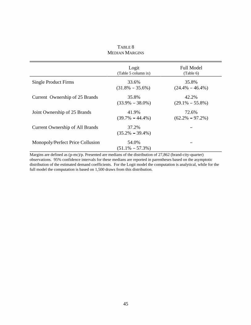
45

TABLE 8MEDIAN MARGINS

Logit(Table 5 column ix)

Full Model(Table 6)

Single Product Firms 33.6%(31.8% % 35.6%)

35.8%(24.4% % 46.4%)

Current Ownership of 25 Brands 35.8%(33.9% % 38.0%)

42.2%(29.1% % 55.8%)

Joint Ownership of 25 Brands 41.9%(39.7% % 44.4%)

72.6%(62.2% % 97.2%)

Current Ownership of All Brands 37.2%(35.2% % 39.4%)

%

Monopoly/Perfect Price Collusion 54.0%(51.1% % 57.3%)

%

Margins are defined as (p-mc)/p. Presented are medians of the distribution of 27,862 (brand-city-quarter)observations. 95% confidence intervals for these medians are reported in parentheses based on the asymptotic distribution of the estimated demand coefficients. For the Logit model the computation is analytical, while for thefull model the computation is based on 1,500 draws from this distribution.

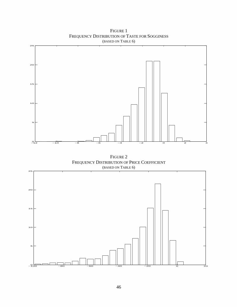
46

−12 −10 −8 −6 −4 −2 0 2 40

5

10

15

20

25

FIGURE 1FREQUENCY DISTRIBUTION OF TASTE FOR SOGGINESS

(BASED ON TABLE 6)

−100 −80 −60 −40 −20 0 200

5

10

15

20

25

FIGURE 2FREQUENCY DISTRIBUTION OF PRICE COEFFICIENT

(BASED ON TABLE 6)

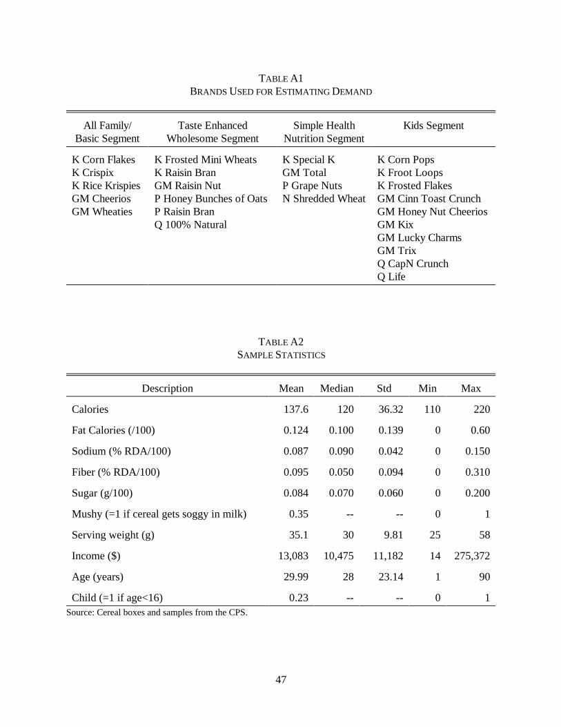
47

TABLE A1BRANDS USED FOR ESTIMATING DEMAND

All Family/Basic Segment

Taste EnhancedWholesome Segment

Simple HealthNutrition Segment

Kids Segment

K Corn FlakesK CrispixK Rice KrispiesGM CheeriosGM Wheaties

K Frosted Mini WheatsK Raisin BranGM Raisin NutP Honey Bunches of OatsP Raisin BranQ 100% Natural

K Special KGM TotalP Grape NutsN Shredded Wheat

K Corn PopsK Froot LoopsK Frosted FlakesGM Cinn Toast CrunchGM Honey Nut CheeriosGM KixGM Lucky CharmsGM TrixQ CapN CrunchQ Life

TABLE A2SAMPLE STATISTICS

Description Mean Median Std Min Max

Calories 137.6 120 36.32 110 220

Fat Calories (/100) 0.124 0.100 0.139 0 0.60

Sodium (% RDA/100) 0.087 0.090 0.042 0 0.150

Fiber (% RDA/100) 0.095 0.050 0.094 0 0.310

Sugar (g/100) 0.084 0.070 0.060 0 0.200

Mushy (=1 if cereal gets soggy in milk) 0.35 -- -- 0 1

Serving weight (g) 35.1 30 9.81 25 58

Income ($) 13,083 10,475 11,182 14 275,372

Age (years) 29.99 28 23.14 1 90

Child (=1 if age<16) 0.23 -- -- 0 1Source: Cereal boxes and samples from the CPS.

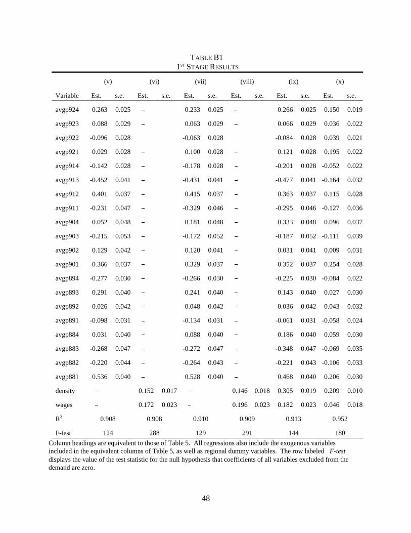
48

TABLE B1

1ST STAGE RESULTS

(v) (vi) (vii) (viii) (ix) (x)

Variable Est. s.e. Est. s.e. Est. s.e. Est. s.e. Est. s.e. Est. s.e.

avgp924 0.263 0.025 % 0.233 0.025 % 0.266 0.025 0.150 0.019

avgp923 0.088 0.029 % 0.063 0.029 % 0.066 0.029 0.036 0.022

avgp922 -0.096 0.028 % -0.063 0.028 % -0.084 0.028 0.039 0.021

avgp921 0.029 0.028 % 0.100 0.028 % 0.121 0.028 0.195 0.022

avgp914 -0.142 0.028 % -0.178 0.028 % -0.201 0.028 -0.052 0.022

avgp913 -0.452 0.041 % -0.431 0.041 % -0.477 0.041 -0.164 0.032

avgp912 0.401 0.037 % 0.415 0.037 % 0.363 0.037 0.115 0.028

avgp911 -0.231 0.047 % -0.329 0.046 % -0.295 0.046 -0.127 0.036

avgp904 0.052 0.048 % 0.181 0.048 % 0.333 0.048 0.096 0.037

avgp903 -0.215 0.053 % -0.172 0.052 % -0.187 0.052 -0.111 0.039

avgp902 0.129 0.042 % 0.120 0.041 % 0.031 0.041 0.009 0.031

avgp901 0.366 0.037 % 0.329 0.037 % 0.352 0.037 0.254 0.028

avgp894 -0.277 0.030 % -0.266 0.030 % -0.225 0.030 -0.084 0.022

avgp893 0.291 0.040 % 0.241 0.040 % 0.143 0.040 0.027 0.030

avgp892 -0.026 0.042 % 0.048 0.042 % 0.036 0.042 0.043 0.032

avgp891 -0.098 0.031 % -0.134 0.031 % -0.061 0.031 -0.058 0.024

avgp884 0.031 0.040 % 0.088 0.040 % 0.186 0.040 0.059 0.030

avgp883 -0.268 0.047 % -0.272 0.047 % -0.348 0.047 -0.069 0.035

avgp882 -0.220 0.044 % -0.264 0.043 % -0.221 0.043 -0.106 0.033

avgp881 0.536 0.040 % 0.528 0.040 % 0.468 0.040 0.206 0.030

density % 0.152 0.017 % 0.146 0.018 0.305 0.019 0.209 0.010

wages % 0.172 0.023 % 0.196 0.023 0.182 0.023 0.046 0.018

R2 0.908 0.908 0.910 0.909 0.913 0.952

F-test 124 288 129 291 144 180

Column headings are equivalent to those of Table 5. All regressions also include the exogenous variablesincluded in the equivalent columns of Table 5, as well as regional dummy variables. The row labeled F-testdisplays the value of the test statistic for the null hypothesis that coefficients of all variables excluded from thedemand are zero.

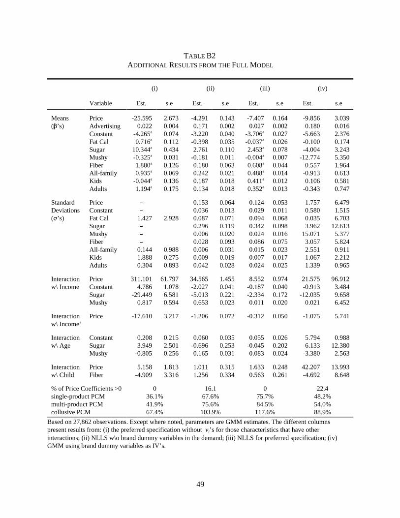
49

TABLE B2

ADDITIONAL RESULTS FROM THE FULL MODEL

(i) (ii) (iii) (iv)

Variable Est. s.e Est. s.e Est. s.e Est. s.e

Means($’s)

PriceAdvertisingConstantFat CalSugarMushyFiberAll-familyKidsAdults

-25.5950.022

-4.265a

0.716a

10.344a

-0.325a

1.880a

0.935a

-0.044a

1.194a

2.6730.0040.0740.1120.4340.0310.1260.0690.1360.175

-4.2910.171

-3.220-0.3982.761

-0.1810.1800.2420.1870.134

0.1430.0020.0400.0350.1100.0110.0630.0210.0180.018

-7.4070.027

-3.706a

-0.037a

2.453a

-0.004a

0.608a

0.488a

0.411a

0.352a

0.1640.0020.0270.0260.0780.0070.0440.0140.0120.013

-9.8560.180

-5.663-0.100-4.004

-12.7740.557

-0.9130.106

-0.343

3.0390.0162.3760.1743.2435.3501.9640.6130.5810.747

Standard Deviations(F’s)

PriceConstantFat CalSugarMushyFiberAll-familyKidsAdults

%

%

1.427%

%

%

0.1441.8880.304

2.928

0.9880.2750.893

0.1530.0360.0870.2960.0060.0280.0060.0090.042

0.0640.0130.0710.1190.0200.0930.0310.0190.028

0.1240.0290.0940.3420.0240.0860.0150.0070.024

0.0530.0110.0680.0980.0160.0750.0230.0170.025

1.7570.5800.0353.962

15.0713.0572.5511.0671.339

6.4791.5156.703

12.6135.3775.8240.9112.2120.965

Interactionw\ Income

PriceConstantSugarMushy

311.1014.786

-29.4490.817

61.7971.0786.5810.594

34.565-2.027-5.0130.653

1.4550.0410.2210.023

8.552-0.187-2.3340.011

0.9740.0400.1720.020

21.575-0.913

-12.0350.021

96.9123.4849.6586.452

Interactionw\ Income2

Price -17.610 3.217 -1.206 0.072 -0.312 0.050 -1.075 5.741

Interactionw\ Age

ConstantSugarMushy

0.2083.949

-0.805

0.2152.5010.256

0.060-0.6960.165

0.0350.2530.031

0.055-0.0450.083

0.0260.2020.024

5.7946.133

-3.380

0.98812.3802.563

Interactionw\ Child

Price Fiber

5.158-4.909

1.8133.316

1.0111.256

0.3150.334

1.6330.563

0.2480.261

42.207-4.692

13.9938.648

% of Price Coefficients >0single-product PCMmulti-product PCMcollusive PCM

036.1%41.9%67.4%

16.167.6%75.6%103.9%

075.7%84.5%117.6%

22.448.2%54.0%88.9%

Based on 27,862 observations. Except where noted, parameters are GMM estimates. The different columnspresent results from: (i) the preferred specification without vi’s for those characteristics that have otherinteractions; (ii) NLLS w\o brand dummy variables in the demand; (iii) NLLS for preferred specification; (iv)GMM using brand dummy variables as IV’s.