Measuring Mortality, Nutritional Status,

and Food Security in Crisis Situations:

SMART METHODOLOGY

Version 1

April 2006

Make everything as simple as possible but not simpler.

—Albert Einstein (1879–1955)

2

Acknowledgments

SMART Methodology Version 1 is the product of many experts working together

over two years. We would like to acknowledge the following individuals who led the

development and drafting of the various components: • Nutrition: Michael Golden • Mortality:

1 Muireann Brennan, Rick Brennan, Reinhard Kaiser, Colleen Mone,

Rose Nathan, Courtland Robinson, Bradley “Woody” Woodruff • Food Security: John Seaman • Nutrisurvey Analytical Software Program: Juergen Erhardt We acknowledge the contributions of the following individuals who provided

technical expertise in methodology development and pilot testing: Frederick (Skip) Burkle, Arabella Duffield, Anne-Sophie Fournier, Debarati Guha-Sapir,

Barbara Macdonald, Richard Garfield, Emmanuel Grellety, Yvonne Grellety, James

King’ori, Nisar Majid, Nancy Mock, Eric Noji, Adam Papendieck, Roger Persichino,

Noreen Prendiville, Claudine Prudhon, Núria Salse, Marie-Sophie Simon, Cathy Skoula. We thank reviewers and all organizations who participated in the process:

Action Against Hunger/USA Action Against Hunger/Spain

Canadian International Development Agency (CIDA)

Centers for Disease Control and Prevention (CDC)

Center for Research on the Epidemiology of Disasters (CRED), University of

Louvain School of Public Health

Columbia University

Department for International Development (DFID),

European Commission (EC)

Fafo Institute for Applied International Studies

Food and Agricultural Organization of the United Nations (FAO)

Food and Nutrition Technical Assistance Project /Academy for Educational Development

(FANTA/AED)

International Rescue Committee (IRC)

Johns Hopkins University (JHU), Bloomberg School of Public Health

Nutrition Information in Crisis Situation/Standing Committee on Nutrition

(NICS/SCN) Save the Children/UK

Save the Children /USA

Technical Assistance to NGOs (TANGO International)

Tulane University, School of Public Health and Tropical

Medicine University of Indonesia

United Nations Children’s Fund (UNICEF)

1 As submitted by Reinhard Kaiser who coordinated with Michael Golden, Juergen Erhardt, and other

experts/organizations.

3

United Nations High Commissioner for Refugees (UNHCR)

U.S. Agency for International Development (USAID) U.S. Department of State/Bureau of Population, Refugees and Migration (State/PRM)

U.S. Department of State/Humanitarian Information Unit (State/HIU)

World Food Program (WFP)

World Health Organization (WHO) Funding from the Canadian International Development Agency (CIDA) is gratefully

acknowledged for the development of SMART Methodology Version 1. Coordination

of the work was led by Susie Villeneuve, UNICEF, and Anne Ralte, USAID.

A special note of appreciation goes to Michael Golden. His commitment to improving

the lives of beneficiaries and ensuring SMART is a practical tool for NGOs and field

practitioners kept the focus on track. 4

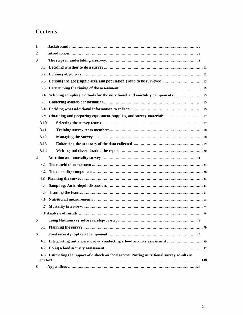
Contents 1 Background ............................................................................................................ 7 2 Introduction ............................................................................................................ 9 3 The steps in undertaking a survey ........................................................................... 11

3.1 Deciding whether to do a survey ................................................................................... 11

3.2 Defining objectives ...................................................................................................... 12

3.3 Defining the geographic area and population group to be surveyed .................................. 13

3.5 Determining the timing of the assessment ...................................................................... 15

3.6 Selecting sampling methods for the nutritional and mortality components ........................ 15

3.7 Gathering available information ................................................................................... 15

3.8 Deciding what additional information to collect .............................................................. 15

3.9 Obtaining and preparing equipment, supplies, and survey materials ................................ 17

3.10 Selecting the survey teams ..................................................................................... 17

3.11 Training survey team members .............................................................................. 18

3.12 Managing the Survey ............................................................................................ 18

3.13 Enhancing the accuracy of the data collected ........................................................... 19

3.14 Writing and disseminating the report ..................................................................... 20 4 Nutrition and mortality survey ............................................................................... 21

4.1 The nutrition component ............................................................................................. 21

4.2 The mortality component ............................................................................................ 28

4.3 Planning the survey ..................................................................................................... 35

4.4 Sampling: An in-depth discussion ................................................................................. 41

4.5 Training the teams ...................................................................................................... 61

4.6 Nutritional measurements ........................................................................................... 65

4.7 Mortality interview ..................................................................................................... 74

4.8 Analysis of results ........................................................................................................ 78 5 Using Nutrisurvey software, step-by-step ................................................................. 79

5.1 Planning the survey .................................................................................................... 79 6 Food security (optional component) ........................................................................ 89

6.1 Interpreting nutrition surveys: conducting a food security assessment .............................. 89

6.2 Doing a food security assessment .................................................................................. 92

6.3 Estimating the impact of a shock on food access: Putting nutritional survey results in context ............................................................................................................................ 109

8 Appendices .......................................................................................................... 123

5

6

1 Background

The SMART Methodology Version 1 provides a basic, integrated method for assessing

nutritional status and mortality rate in emergency situations. It provides the basis for

understanding the magnitude and severity of a humanitarian crisis. The optional food

security component provides the context for nutrition and mortality data analysis. The July 2002 SMART workshop recommended ( www.smartindicators.org) the

development of a generic method that provides timely and reliable data in a standardized

way for prioritizing humanitarian assistance for policy and program decisions. This is the

first coordinated effort by the international humanitarian community to provide

standardized data that is accurate and reliable for decision making. The SMART Methodology Version 1 draws from core elements of several existing methods and current best practices. Recommendations are based on varying degrees of evidence: 1) methods for which there is clear scientific evidence to support its recommendation, 2) practices that empirical evidence from field work suggest will lead to scientifically valid conclusions, and 3) practices that are considered reasonable and valid but for which more evidence is needed. In particular, the evidence for recommending the particular method for assessing mortality rate is limited, and there is need for more field experience and analysis. For nutrition, the method builds upon well-established methods. In particular, the Save the Children/UK Emergency Nutrition

Assessment: Guidelines for Field Workers 2 and SC/UK colleagues provided the sound

technical foundation for building a generic method that could be applied in all

emergencies. For food security, although there is not yet an agreed method or best practice, the

Household Economy Approach (Livelihood Method) has worked well in predicting

quantitatively how an event, such as crop failure or price change, is likely to affect

people’s ability to get food. It gives an estimate of who will be affected, how severely

they will be affected, and when they will be affected. Other methods do not give this

quality of information. In addition, the method developed especially for SMART

Methodology Version 1 is the simplest, practical version of the Household Economy

Approach that still provides the most essential data that can be collected alongside the

nutrition and mortality survey. A practical consideration that initiated the development of the SMART method, and

guided the decision process in its development, is that nongovernmental organization

(NGO) partners should be able to collect these data with ongoing nutrition surveys with

a minimum of added burden to their programs. In addition, the method’s level of

difficulty is a conscientious balance between technical soundness and simplicity for

rapid assessment of acute emergencies to obtain early, accurate, quantitative profiles of a

population’s nutritional status and mortality rate. For these reasons, the SMART method is iterative, with continuous upgrading and

building on this basic version, informed by research, experience, and current best 2 Emergency Nutrition Assessment: Guidelines for Field Workers, Save the Children, U.K., 2004.

7

practices. For example, cause of death and other related indicators will be reviewed for

potential inclusion in later versions. All partners and relief organizations are encouraged

to use SMART Methodology Version 1 to inform this dynamic process and the research

agenda. In countries where standardized methodologies are being used already, effort

should be made to comply with the SMART method as far as possible. Version 1 is not intended to be a comprehensive manual that covers all aspects of all

surveys, nor is it meant to be inflexible. Efforts have been to provide detailed instructions

where possible, yet allow sufficient flexibility to cover the many and varied situations

that arise in the field. Intended users are host-government partners and humanitarian organizations. Version 1 is

intended as a practical tool that can be used by NGO field workers with technical support

and training. The SMART Initiative is establishing a comprehensive capacity building

and support system that will be accessible to all partners. This will expand the use of the

standardized method among national and international agencies, improve data quality,

and enable decision making based on accurate data. 8

2 Introduction The basic indicators for assessing the severity of a crisis are the mortality, or death

rate, and the nutritional status of the population. These are both estimated by

conducting a survey of the affected population. To know the magnitude of the problem we also need to know the population size and, if

possible, the demographic characteristics of the population. A high proportion of

malnourished in a small population is normally of less magnitude than a lower

proportion of malnourished in a large population. The scale and type of intervention will

depend upon the magnitude of the emergency rather than simply on the prevalence of

malnutrition. To understand the reasons for the crisis and to plan and implement appropriate relief, the

usual situation for that population, the evolution of the changes, and the context in which

the emergency has arisen each needs to be considered. There are many sources of

information that are relevant in putting the crisis in context and that may affect the types

of response that are appropriate. Cultural, political, economic, anthropological, medical,

nutritional, topographical, climatic, seasonal, and other factors can all be important. The

effects of these factors on livelihoods and the ability of the affected population to cope at

a household level are assessed using a food security survey. To be useful, the information has to be relatively easy to collect, reliable, and

accurate. This manual is designed to provide agencies with the basic tools to collect

the data necessary for planning direct interventions in an emergency setting. 3

The manual is divided into two sections: the assessment of nutritional status and

death rates, and the examination of the food security situation. These data should be collected from the same population simultaneously by conducting

surveys. The data are then integrated with estimates of the population size to provide an

overall picture of the scale of the crisis and the required response. It is not difficult to conduct a survey, but there are a number of critical points that have to

be correct for the results to be valid. It does require planning, training, supervision of

staff, interaction with the community, and at least a basic understanding of the concepts

of epidemiology and statistics. A survey should provide information that is accurate and reflects the current situation—

not the situation at some time in the past. It should be relatively simple to conduct. The

results should be available in time for the data to be useful for the intervention. Complex

surveys that attempt to answer many questions and give a complete picture are difficult

to conduct, analyze, and interpret. They also cost a lot and require special expertise. The

information is often outdated by the time the survey is finished, and it is not easily 3

Collecting and analyzing data for advocacy, policymaking, and other such purposes is also necessary;

methods for collecting data for these purposes may be different from the methods advocated in this manual.

Because this manual is designed for use by field staff without special epidemiological knowledge or experience, it is limited to the methods that yield reliable information for programming.

9

repeated to give an ongoing picture of changes. It is nearly always better to do a

relatively simple survey that answers only the pressing, critical questions, and that can be

repeated as the situation evolves. Each additional piece of data gathered, even if it is

relatively simple itself, degrades the quality and care with which the critical data are

gathered and delays the survey. This manual is designed to be used in conjunction with the accompanying

software, Nutrisurvey for SMART, which is freely available from

www.nutrisurvey.de/ena/ena.html. 10

3 The steps in undertaking a survey The steps we are going to consider for mortality, nutrition, and food security surveys are

as follows:

• deciding whether to do a survey

• defining the objectives

• defining the geographic area and population group(s) to be surveyed

• meeting the community leaders and local authorities

• determining when the assessment is to be undertaken

• selecting the sampling method and clusters

• gathering available information

• deciding what additional information to collect

• obtaining and preparing equipment, supplies, and survey materials

• selecting the survey teams

• training survey team members

• managing the survey

• enhancing the accuracy of data collected

• writing the report and presenting it to interested parties

This section of the manual describes those steps that are common to all the components

of the survey. Steps that differ for the different components are summarized and

explained in other sections.

3.1 Deciding whether to do a survey The decision to undertake an assessment is usually made in conjunction with the

government, partner agencies, and donors. To prevent unnecessary repetition or overlap

by different agencies, it is always important to share information about when and where

you plan to undertake a survey. Surveys are usually much more informative if they are

coordinated so that data from several agencies, geographic areas, or population groups

can be examined together to give a wider perspective on the situation. Conducting an assessment is expensive and time-consuming, so before starting

you should consider the following points:

• Are the results crucial for decision making? If a population’s needs are obvious,

immediate program implementation takes priority over doing a survey, and the

survey should be deferred. For example, after a natural disaster, such as a flood,

where it is clear that the population’s food stocks have been destroyed, the current

nutritional status may reflect the pre-disaster state. In dramatically changing 11

situations, nutritional and mortality surveys are not helpful guides to current or

future needs. If large numbers of malnourished children are present at a center,

implementation of relief programs should not be delayed until a survey is

conducted. The Sphere minimum standards require that a nutrition assessment be

conducted when a targeted feeding program is implemented (The Sphere Project

2004); however, this does not mean the program should be delayed until after the

survey is completed if the need is clear. Where such programs exist, periodic

surveys should be conducted. If another agency has recently carried out a

nutrition assessment in the same area, that data should be used rather than

repeating the survey.

• It should be anticipated that the results will lead to action: there is little point of

doing a survey if you know a response will not be possible. If the agency cannot

itself implement a program where needed, the results must be useful in advocating

for a response.

• Is the affected population accessible? Insecurity or geographical constraints may

result in limited access to the population of interest. If this is extreme, a survey

cannot be conducted.

3.2 Defining objectives Clear objectives make it much easier for your team, the population, and donors to understand

why the survey is being conducted. This should be clearly stated at the outset. Emergency nutrition assessments are usually conducted to assess the severity of the

situation by quantifying the acute malnutrition and mortality in a given population at a

defined point in time. This is done by estimating the prevalence of wasting and edema in

children aged 6–59 months and the death rate of the entire population. With an estimate

of population size, the proportions of malnourished and the death rate give an estimate

of the absolute number of malnourished in the community and how many have died in

the recent past. These figures indicate the magnitude of the problem. The estimates,

together with previous surveys, food security and contextual data, also indicate the

urgency of the situation and how it may evolve in the future. Where the survey is undertaken during a stable period, the data can be used to establish a

baseline from which future changes can be monitored over time. Undertaking a nutrition and mortality survey provides an opportunity to collect additional

information that can be critical in deciding which interventions are most important.

Immunization and nutrition program coverage, vitamin A, iodine, anemia, or other

micronutrient deficiency, disease morbidity, trauma experience, cause of death,

demographic, migration, and many other variables can all be important. It is critical to understand that each additional piece of data collected degrades the

accuracy of the whole dataset and prolongs and complicates the survey. Thus, any

additional information to be collected should be clearly stated and justified in the

objectives and have a realistic prospect of leading to a meaningful intervention. Nevertheless, such data are usually needed. Consideration has to be given to whether the

information could be collected more efficiently in other ways (for example from health

12

clinics, sentinel sites or a surveillance system), or whether it would be better to conduct a

separate survey to collect the supplementary information. If additional information is to

be included in the survey it must be quickly and reliably obtainable during a short visit to

the household.

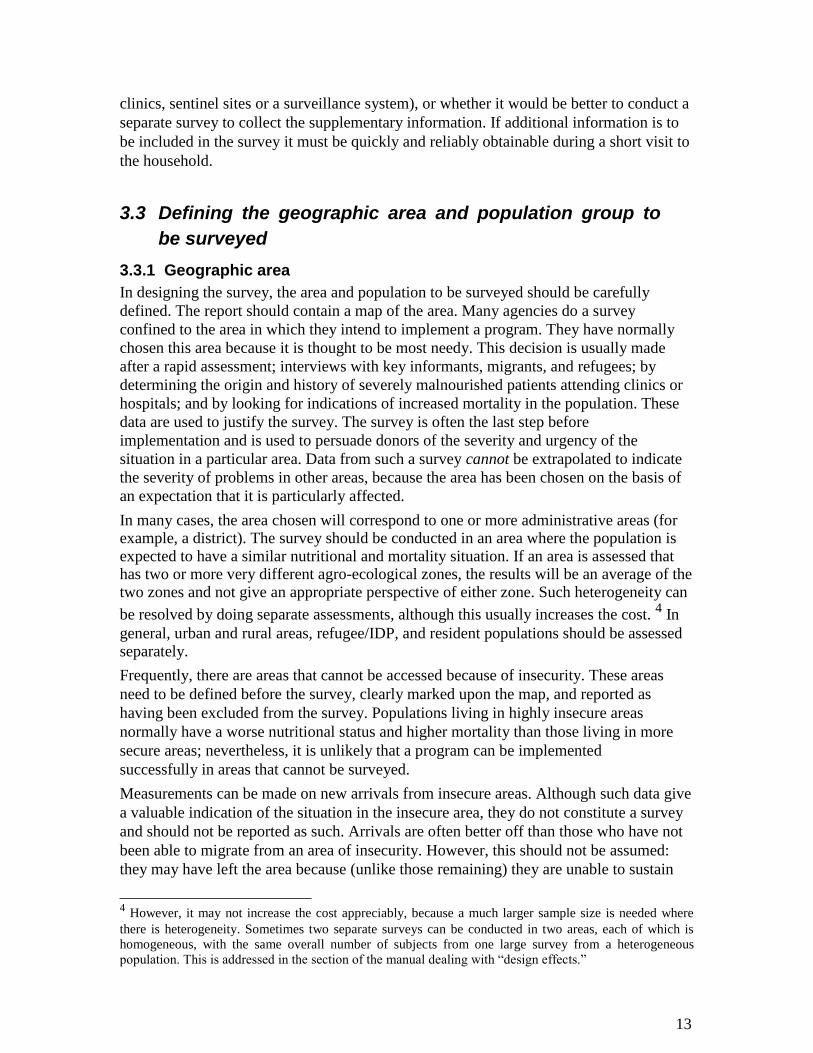
3.3 Defining the geographic area and population group to

be surveyed 3.3.1 Geographic area In designing the survey, the area and population to be surveyed should be carefully

defined. The report should contain a map of the area. Many agencies do a survey

confined to the area in which they intend to implement a program. They have normally

chosen this area because it is thought to be most needy. This decision is usually made

after a rapid assessment; interviews with key informants, migrants, and refugees; by

determining the origin and history of severely malnourished patients attending clinics or

hospitals; and by looking for indications of increased mortality in the population. These

data are used to justify the survey. The survey is often the last step before

implementation and is used to persuade donors of the severity and urgency of the

situation in a particular area. Data from such a survey cannot be extrapolated to indicate

the severity of problems in other areas, because the area has been chosen on the basis of

an expectation that it is particularly affected. In many cases, the area chosen will correspond to one or more administrative areas (for example, a district). The survey should be conducted in an area where the population is expected to have a similar nutritional and mortality situation. If an area is assessed that has two or more very different agro-ecological zones, the results will be an average of the two zones and not give an appropriate perspective of either zone. Such heterogeneity can

be resolved by doing separate assessments, although this usually increases the cost. 4 In

general, urban and rural areas, refugee/IDP, and resident populations should be assessed separately. Frequently, there are areas that cannot be accessed because of insecurity. These areas

need to be defined before the survey, clearly marked upon the map, and reported as

having been excluded from the survey. Populations living in highly insecure areas

normally have a worse nutritional status and higher mortality than those living in more

secure areas; nevertheless, it is unlikely that a program can be implemented

successfully in areas that cannot be surveyed. Measurements can be made on new arrivals from insecure areas. Although such data give

a valuable indication of the situation in the insecure area, they do not constitute a survey

and should not be reported as such. Arrivals are often better off than those who have not

been able to migrate from an area of insecurity. However, this should not be assumed:

they may have left the area because (unlike those remaining) they are unable to sustain

4 However, it may not increase the cost appreciably, because a much larger sample size is needed where

there is heterogeneity. Sometimes two separate surveys can be conducted in two areas, each of which is

homogeneous, with the same overall number of subjects from one large survey from a heterogeneous

population. This is addressed in the section of the manual dealing with “design effects.”

13

themselves or have been rejected by the rest of the population. Often, relief programs

have to take account of such migration from insecure areas that have not been, and cannot

be, surveyed.

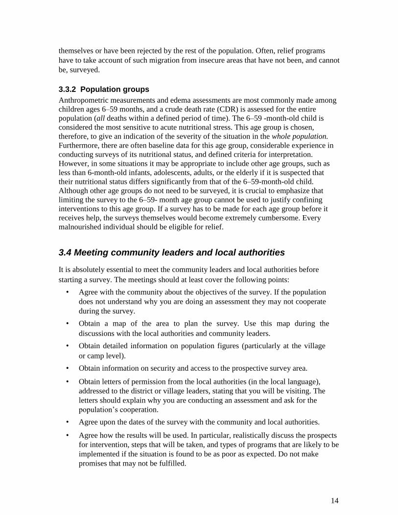
3.3.2 Population groups Anthropometric measurements and edema assessments are most commonly made among

children ages 6–59 months, and a crude death rate (CDR) is assessed for the entire

population (all deaths within a defined period of time). The 6–59 -month-old child is

considered the most sensitive to acute nutritional stress. This age group is chosen,

therefore, to give an indication of the severity of the situation in the whole population.

Furthermore, there are often baseline data for this age group, considerable experience in

conducting surveys of its nutritional status, and defined criteria for interpretation.

However, in some situations it may be appropriate to include other age groups, such as

less than 6-month-old infants, adolescents, adults, or the elderly if it is suspected that

their nutritional status differs significantly from that of the 6–59-month-old child.

Although other age groups do not need to be surveyed, it is crucial to emphasize that

limiting the survey to the 6–59- month age group cannot be used to justify confining

interventions to this age group. If a survey has to be made for each age group before it

receives help, the surveys themselves would become extremely cumbersome. Every

malnourished individual should be eligible for relief.

3.4 Meeting community leaders and local authorities It is absolutely essential to meet the community leaders and local authorities before

starting a survey. The meetings should at least cover the following points:

• Agree with the community about the objectives of the survey. If the population

does not understand why you are doing an assessment they may not cooperate

during the survey.

• Obtain a map of the area to plan the survey. Use this map during the

discussions with the local authorities and community leaders.

• Obtain detailed information on population figures (particularly at the village

or camp level).

• Obtain information on security and access to the prospective survey area.

• Obtain letters of permission from the local authorities (in the local language),

addressed to the district or village leaders, stating that you will be visiting. The

letters should explain why you are conducting an assessment and ask for the

population’s cooperation.

• Agree upon the dates of the survey with the community and local authorities.

• Agree how the results will be used. In particular, realistically discuss the prospects

for intervention, steps that will be taken, and types of programs that are likely to be

implemented if the situation is found to be as poor as expected. Do not make

promises that may not be fulfilled. 14

3.5 Determining the timing of the assessment The exact dates of the assessment should be chosen with the help of community leaders

and local authorities to avoid market days, local celebrations, food distribution days,

vaccination campaigns, or other times when people are likely to be away from home.

Roads may be impassable during the rainy season. In agricultural areas, women may be

in the fields for most of the day during ground preparation, planting, or harvesting.

Healthy children are more likely to accompany adults to the market or the fields and are

less likely to be in the home than ill or malnourished children. The survey results could

be wrong if only children who were at home at the time of the survey team’s visit are

sampled. Wherever possible, community leaders should inform the villages chosen to be

surveyed in advance. There needs to be sufficient time allocated for preparation and literature review,

training, pilot testing, community mobilization, data collection, analysis, and reporting.

3.6 Selecting sampling methods for the nutritional and

mortality components The basic principle for selecting the households that will be visited is that every child in

the whole study population should have an equal chance of being selected for the

nutritional survey, and every person for the mortality survey. If, at any stage, the

recommended method has to be changed for practical reasons, then those in charge have

to consider whether every household and child is equally likely to be sampled. The three commonly used methods are simple random sampling, systematic

random sampling and cluster sampling.

3.7 Gathering available information Before starting the survey, it is important to learn as much about the population as

possible from existing sources, including population characteristics and figures, previous

surveys and assessments, health statistics, food security information, situation reports

(security and political situation), maps, and anthropological, ethnic, and linguistic

information. Only after these data are gathered can judgment be made about any

additional information that should be collected.

3.8 Deciding what additional information to collect The data collected must correspond to the assessment’s objectives. The mortality and nutritional data are gathered at the same time from the same

households. Food security data are not collected from households, but through

key-informant interviews with people or groups from the same community.

15

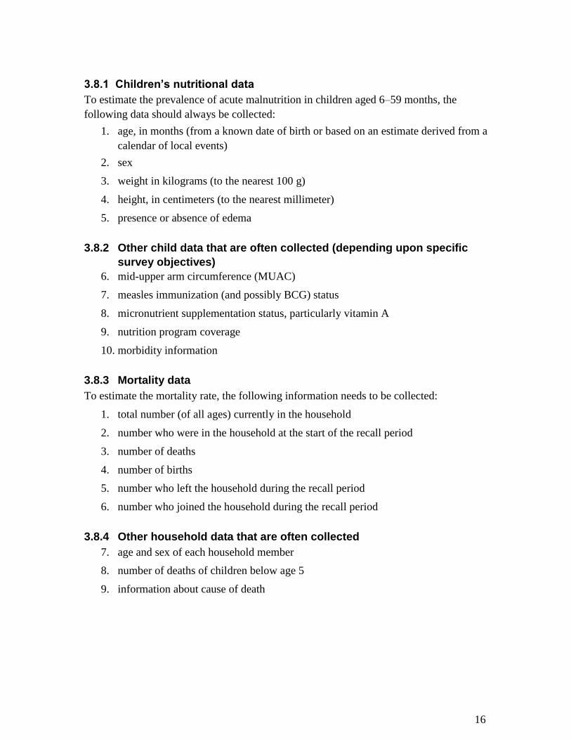
3.8.1 Children’s nutritional data To estimate the prevalence of acute malnutrition in children aged 6–59 months, the

following data should always be collected:

1. age, in months (from a known date of birth or based on an estimate derived from a

calendar of local events)

2. sex

3. weight in kilograms (to the nearest 100 g)

4. height, in centimeters (to the nearest millimeter)

5. presence or absence of edema

3.8.2 Other child data that are often collected (depending upon specific

survey objectives) 6. mid-upper arm circumference (MUAC)

7. measles immunization (and possibly BCG) status

8. micronutrient supplementation status, particularly vitamin A

9. nutrition program coverage

10. morbidity information

3.8.3 Mortality data To estimate the mortality rate, the following information needs to be collected:

1. total number (of all ages) currently in the household

2. number who were in the household at the start of the recall period

3. number of deaths

4. number of births

5. number who left the household during the recall period

6. number who joined the household during the recall period

3.8.4 Other household data that are often collected 7. age and sex of each household member

8. number of deaths of children below age 5

9. information about cause of death

16

3.8.5 Food security Food security data are collected at the same time from the same population, but by

separate teams using different methods. Food security and other questions are not added

to the nutrition/mortality survey. Food security data comes mainly from key informant

interviews using the household economy approach, market assessments and

observations. The training and skills required to collect these data are different from

those required for nutritional and mortality assessment (see section 4).

3.9 Obtaining and preparing equipment, supplies, and

survey materials Measuring material, scales, and height boards should be in good condition. During the

survey, scales should be checked each day against a known weight (standard weight).

If the measure cannot be made to match the weight by adjustment of the zero and span

controls, the equipment should not be used. Spare equipment is needed to allow for

damage or loss. Equipment and supplies needed for the survey include transport, fuel, paper and pens, per

diem, and recording forms. Copies of questionnaires, absentee forms and forms for referral of moderately or severely

malnourished cases to supplementary feeding and therapeutic feeding programs (if they

exist) should be prepared.

3.10 Selecting the survey teams 3.10.1 Nutrition and mortality survey teams

For the nutrition and mortality components, each survey team has a minimum of three

people. Two make the anthropometric measurements, while one records data and serves

as the team leader. The team leader is responsible for the quality and reliability of the

data collected. The same team members can sometimes take both the anthropometry and

conduct the mortality interview. However, it is usually better to have a fourth team

member who interviews the head of household to collect the census and mortality data. To make implementation more efficient and rapid, a respected member of the community

should be asked to participate with each team. He/she will know the village and be able

to guide the team, locating households. The community member can more easily learn

the whereabouts of absent households, and perform the often vital function of translation.

If for some reason the community member does not speak the local dialect, it may be

necessary to include a translator on the team. Team members do not have to be health professionals. In fact, anyone from the

community can be selected and trained. They need to be fit, as there is usually a lot of

walking. They should have a relatively high level of education, as they will need to read

and write fluently, count accurately. Ideally, they will speak the local language. Women

generally have much more experience dealing with young children and should usually 17

make up the majority of the team. In some cultures, it is necessary to have at least one

male member of the team to interview male heads of household. Most importantly,

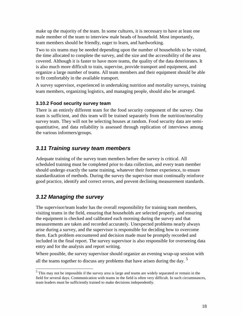
team members should be friendly, eager to learn, and hardworking. Two to six teams may be needed depending upon the number of households to be visited,

the time allocated to complete the survey, and the size and the accessibility of the area

covered. Although it is faster to have more teams, the quality of the data deteriorates. It

is also much more difficult to train, supervise, provide transport and equipment, and

organize a large number of teams. All team members and their equipment should be able

to fit comfortably in the available transport. A survey supervisor, experienced in undertaking nutrition and mortality surveys, training

team members, organizing logistics, and managing people, should also be arranged.

3.10.2 Food security survey team There is an entirely different team for the food security component of the survey. One

team is sufficient, and this team will be trained separately from the nutrition/mortality

survey team. They will not be selecting houses at random. Food security data are semi-

quantitative, and data reliability is assessed through replication of interviews among

the various informers/groups.

3.11 Training survey team members Adequate training of the survey team members before the survey is critical. All

scheduled training must be completed prior to data collection, and every team member

should undergo exactly the same training, whatever their former experience, to ensure

standardization of methods. During the survey the supervisor must continually reinforce

good practice, identify and correct errors, and prevent declining measurement standards.

3.12 Managing the survey The supervisor/team leader has the overall responsibility for training team members,

visiting teams in the field, ensuring that households are selected properly, and ensuring

the equipment is checked and calibrated each morning during the survey and that

measurements are taken and recorded accurately. Unexpected problems nearly always

arise during a survey, and the supervisor is responsible for deciding how to overcome

them. Each problem encountered and decision made must be promptly recorded and

included in the final report. The survey supervisor is also responsible for overseeing data

entry and for the analysis and report writing. Where possible, the survey supervisor should organize an evening wrap-up session with

all the teams together to discuss any problems that have arisen during the day. 5

5 This may not be impossible if the survey area is large and teams are widely separated or remain in the

field for several days. Communication with teams in the field is often very difficult. In such circumstances,

team leaders must be sufficiently trained to make decisions independently.

18

Before leaving the field, each team leader should review and sign all forms to ensure that

no pieces of data have been left out. If there were people absent from the house during

the day, the team should return to the household at least once before leaving the area. It is also the duty of the survey supervisor to regularly supervise teams in the field. It is

particularly important to check cases of edema, as there are often no cases seen during the

training and some team members may therefore be prone to mistaking a fat child for one

with edema (particularly with younger children). The supervisor should note teams that

report a lot of edema, confirm measles and death cases, and visit some of these children

to verify their status. It is very important not to overwork survey teams. There is a lot of walking involved in

carrying out a survey, and when people are tired, they may make mistakes or fail to

include more distant houses selected for the survey. The supervisor must make sure the

team has enough time to take appropriate rest periods and that it has refreshments.

3.13 Enhancing the accuracy of the data collected Each evening, or during the next day while the teams are in the field, the supervisor

should arrange for data to be entered into the computer. Recording errors, unlikely

results, and other problems with the data may become clear at this stage. The Nutrisurvey

software will automatically flag abnormal values as data are entered. Each morning,

before the teams set out for the day, there should be a short feedback session. If any team

is getting a large number of “flagged” results, the supervisor should accompany that team

the next day. If the results are very different from those obtained by the other teams, it

may be necessary to repeat the cluster from the day before. Team leaders and survey supervisor should record all important points in a notebook as

soon as possible (e.g., during breaks or at base in the evening), including observations,

ideas, problems, actions taken to address these problems, and the reasoning behind any

decisions taken. Each note should be labeled with the date, location, and names of

relevant people. Apart from the evening and morning meetings, survey team members should be encouraged

to regularly discuss their experiences and findings together. This often brings out important

points, and sometimes shows where survey methods need to be modified. If possible, at each household the team leader should calculate or look up in a table the

percentage weight-for-height (WFH) median score for each child and classify the child’s

nutrition status. This should certainly be done for any child who appears to be

malnourished. When a malnourished child is identified he or she should be referred, on

the spot, to the nearest health or nutrition facility. Ideally, this will be a therapeutic or

supplementary feeding program. If these are not available, the supervisor should urge the

parents to take the child to the nearest health facility, providing a referral slip upon which

the name, height, weight, percentage WFH, and diagnosis is written. The team collecting the food security data should also attend the evening wrap-up

meetings. From their experiences conducting interviews, they will often be able to

contribute valuable anthropological insight into the problems encountered by the other

survey teams. They will also benefit from meeting a variety of the teams working in

19

different villages in the area, enabling them to assess how representative the villages

selected for key informant interviews are of the entire area, and if such interviews

should be replicated elsewhere.

3.14 Writing and disseminating the report

The final part of a survey is writing and disseminating the report. The results of the

survey should be presented in a standard format so that different surveys can be

compared, and no important information should be left out. After being introduced to the

standard format, it is also becomes much easier for readers to find particular pieces of

information in the report. The Nutrisurvey software has been designed to automatically present all important data in

standard format under standard section headings. The results of an emergency survey

must be released and disseminated as soon as possible to prevent any delay in the

intervention. Reports for emergency nutrition and mortality surveys should be available

no later than one week after completing data collection. Baseline survey reports may not

be needed so soon. The report melds data from the nutrition and mortality components with the food security

data to give an overall picture of the situation within the survey area. The quantitative

data on anthropometry and crude death rates require context, and the report is designed to

provide this, partially through a discussion of background information and previous

surveys, but mainly through the presentation of the food security data gathered from the

same area during same time period. All together, the report is intended to be used to make

recommendations and formulate plans of action for intervention.

20

4 Nutrition and mortality survey

4.1 The nutrition component 4.1.1 Why do a nutrition survey? Whether due to starvation, loss of appetite, malabsorption, or psychological causes,

children who have not taken a sufficient amount of food do not grow; and under more

severe circumstances, they lose weight. Decreased growth rate is assessed by

comparing the ratio of a child’s height to weight to a reference standard for the child’s

age. For an individual, these measurements are used to decide whether the person is

admitted to a supplementary feeding program or treated for severe malnutrition. At the

population level, the same measurements are used in the survey to estimate what

proportion of a population as a whole is moderately or severely malnourished. Malnutrition in the context of this manual takes three forms: 1) failure to grow results in

height stunting; 2) loss of body tissue results in wasting, and 3) accumulation of fluid

results in nutritional edema (also called kwashiorkor, or hunger edema). The prevalence

of each of these is assessed during a nutrition survey by recording age, measuring weight

and height, and examining for edema. Other forms of malnutrition, such as micronutrient deficiency, are not usually assessed

during a nutrition/mortality survey, even though they may be very important causes of

morbidity and mortality. Most micronutrient deficiency diseases do not cause stunting or

wasting, and their prevalence cannot be determined from anthropometric measurements. 6

4.1.2 Populations for anthropometric surveys: 6–59-month-old children In emergencies, wasting among children aged 6–59 months is used as a proxy indicator

for the general health and wellbeing of the entire community. This assumes that

children aged 6–59 months are the most vulnerable group in the society, at least as

vulnerable as each of the other age groups. This is usually, but not always, true. In practice, this group is much easier to measure than other population groups. Young

children are generally at home, the parents are usually concerned about their children

and willing for them to be measured, and they are not embarrassed by (nor are there as

many cultural restrictions about) taking off their clothes. Also, the equipment needed is

not as cumbersome as that for older age groups. There are a few other very basic reasons why children aged 6–59 months are a good

group to survey. First of all, policymakers are used to seeing and acting upon this type of

data. There is a lot of experience with surveys of this age group, affording those using the

data to make decisions the opportunity to compare the new survey with previous surveys.

Furthermore, there is not yet international agreement on the anthropometric indicators

and cut-off points used to assess acute malnutrition in adolescents, adults, pregnant and

lactating mothers, and older people.

6 An important corollary of this is that if the result of the anthropometric survey does not give rise to

concern, there could still be major undetected micronutrient deficiency in the population that is an

underlying cause of illness and death.

21

It must be reiterated that surveys of children aged 6–59 months are used to indicate the

situation of the whole population and not just young children, and restricting data

collection to this group should in no way be understood as justification for confining

relief to them.

4.1.3 When to measure the nutritional status of people over age 5 Surveys including other age groups are more complex and require greater technical

expertise than for children aged 6–59 months. However, it may be appropriate to

assess the nutritional status of other age groups in the following circumstances:

1. When there is a relative increase in the crude death rate (CDR) compared to zero

to 5 death rates. The 0–5 death rate is generally about twice the CDR. A

disproportionate increase in the CDR suggests that there is a particular problem in

older age groups so that the 6–59-month age group is no longer a good indicator

of the stress of the whole population.

2. When there is reasonable doubt that the nutrition status of young children reflects

the whole population’s nutritional situation. For example, in populations where

cultural traditions give preference to the feeding of young children, or when there

is a high prevalence of HIV, older adults may be more severely affected.

3. When many adults or older children present themselves to selective

feeding programs or health facilities with malnutrition.

4. When credible anecdotal reports of frequent adult or adolescent malnutrition

are received.

5. When the data are required as an advocacy tool to persuade policymakers to

address the needs of other age groups. Ideally, this should not be necessary. The methods for sampling and measuring other age groups are the same as those for the

6–59-month age group described in this manual. Infants less than 6 months can be

included in the survey, but there are particular difficulties related to the accuracy and

precision of the measurements.

4.1.4 Nutrition indices and indicators To determine the nutrition status of an individual, the weight, height, age, and presence of

edema are recorded. The relationship of these measurements to each other is compared to

international reference standards. The nutrition surveys are designed with respect to three

indices: height-for-age (HFA), weight-for-height (WFH), and weight-for-age (WFA). Growing children get taller, and the height of a child in relation to a “standard” child of the

same age gives an indication of whether the growth has been normal or not. This index of

growth is called height-for-age. Children who have a low HFA are referred to as stunted.

Growth is a relatively slow process, and if a child of normal height stops growing it takes a

long time for that child to fall below the cutoff point for stunting. 7 For this reason, HFA is

often used to indicate long-standing or chronic malnutrition. If the 7 A child who is 100% of normal growth who falters to 70% of normal will take up to half his life to fall

below the usual cutoff point and be labeled as moderately stunted. Thus, a 1-year-old child who is gaining

height at 70% of normal will not be designated as stunted for six months.

22

insult that led to stunting is in the past, it is possible that the current growth rate is

actually normal (although this is unusual without a change in the family circumstances).

Stunting may also be due to intrauterine growth retardation followed by normal postnatal

growth. A child getting taller will also gain weight if body proportions remain normal. A thin

child will weigh less than a normal child of the same height. Weight-for -height is a

measure of how thin (or fat) the child is. Because weight gain or loss is much more

responsive to the present situation, WFH is usually taken to reflect recent nutritional

conditions. Being excessively thin is called wasting. It is also often termed “acute

malnutrition,” although individual children may have been thin for a long time. An

advantage of using WFH to assess the nutritional state is that it does not involve age; in

many poor populations, age is not known and is difficult to estimate reliably,

especially in emergency situations. Neither stunted nor wasted children weigh as much as normal children of the same age.

Weight-for-age is thus a composite index, which reflects both wasting and stunting, or

any combination of both. In practice about 80% of the variation in WFA is related to

stunting and about 20% to wasting. It is not a good indication of recent nutritional stress.

It is used because it is an easy measurement to take in practice, and can be used to

follow individual children longitudinally in the community. Mid-upper arm circumference (MUAC) is also sometimes measured. It directly assesses

the amount of soft tissue in the arm and is another measure of thinness (or fatness), like

WFH. Although it is easier to measure MUAC than WFH, it is more difficult to make a

precise measurement, it is not standardized for age, and the cutoff points are not

universally accepted. Nevertheless, MUAC is the best index to use in the community (for

screening) to identify individual children in need of referral for further assessment or

treatment. Because MUAC is used in this way in the community, it is useful to know the

relationship between WFH and MUAC in a particular community to establish a full

nutrition program including screening. This is why MUAC is sometimes included in the

data collected in a survey. MUAC data are often not reported or emphasized in a report,

and decisions are not usually based upon these data alone. WFH, HFA, and WFA are calculated for individuals and groups using the Nutrisurvey

software. 8 Users of this manual are not expected to have to calculate these values

without the aid of a computer.

4.1.5 The reference population curves To assess malnutrition as determined by WFH, WFA, and HFA, individual measurements

are compared to an international reference standard. At present that standard is derived

from surveys undertaken in the United States (NCHS/WHO/CDC reference table, WHO

1983). New reference values are currently being compiled, and SMART will adopt these

new standards whenever they become available. However, until many surveys have been

conducted with the new standards and the humanitarian community has become used to

interpreting the results, SMART will continue to report the prevalence of malnutrition

using existing and new standards.

8 The software “Epiinfo” can also be used to calculate the nutritional variables.

23

The reference values should not be considered “ideal”; they are simply used as a standard

to compare nutritional status in different regions, and in populations over time. It is a

standard in the same way that the meter or the kilogram are standards used to measure

length or weight. Each team should have a copy of the reference standards tables so that during the survey

they can identify children who need immediate referral to a nutrition or health facility.

4.1.6 Expression of nutrition indices Anthropometric indices are usually expressed in two ways: as the percentage of the

median value of the reference standard, or as z-scores derived from the reference

standard.

4.1.6.1 The percentage of the median

The percentage of the median 9 WFH (often written WHM

10 ), compares the weight of

the child to the median weight of children of the same height in the reference population (see box 1). The calculation of WHM for each child is based on the child’s weight and

the median weight for children of the same height (and sex) in the reference population: WHM = the child’s weight divided by the reference median weight × 100

Box 1. Example WHM calculation

In a nutritional survey, a male child 92cm tall weighs 12.1kg. The median weight for

boys in the reference population who are 92cm tall is 13.7kg. WHM = 12.1/13.7 × 100 = 88.3%

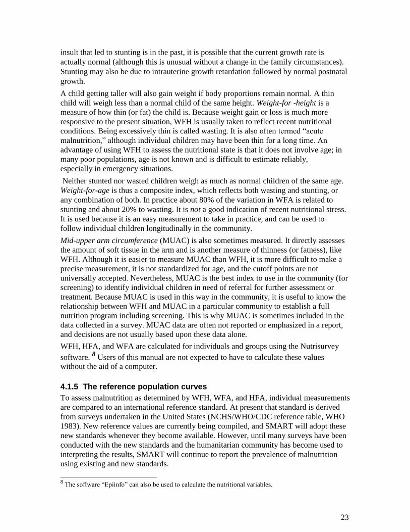
4.1.6.2 The z-score A z-score is another measure of how far a child is from the median WFH of the reference

(often written WHZ) . In the reference population, all children of the same height are

distributed about the median weight, some heavier and some lighter. For each height

group, there is a standard deviation among the children of the reference population. This

standard deviation is expressed as a certain number of kilograms at each height. The z-

score of a child being measured is the number of standard deviations (of the reference

population) the child is away from the median weight of the reference population at that

age group. This is illustrated in figure 1 below: 9 The median is a type of average. It is used instead of the mean because the standard population is not normally distributed. This was a problem with bottle feeding making some of these children obese so that the upper half of the distribution is slightly more “spread out” than the lower half. The median is simply the middle value that has half the population above and half below a given value.

10 It is also sometimes written as “WHP.” However, this abbreviation is also used for WFH expressed as a centile value, because of common misuse of “percentile” in place of centile. The abbreviation has been changed to WHM to avoid confusion.

24

Weights of boys 80 cms in length in reference population 16

12 ch

ild

ren

8

% o

f

4

0 7-7.4 7.5- 8-8.4 8.5- 9-9.4 9.5- 10- 10.5- 11- 11.5- 12- 12.5- 13- 13.5- 14- 7.9 8.9 9.9 10.4 10.9 11.4 11.9 12.4 12.9 13.4 13.9 14.4

Weight (kgs)

Figure 1. Reference curve used to derive a z-score

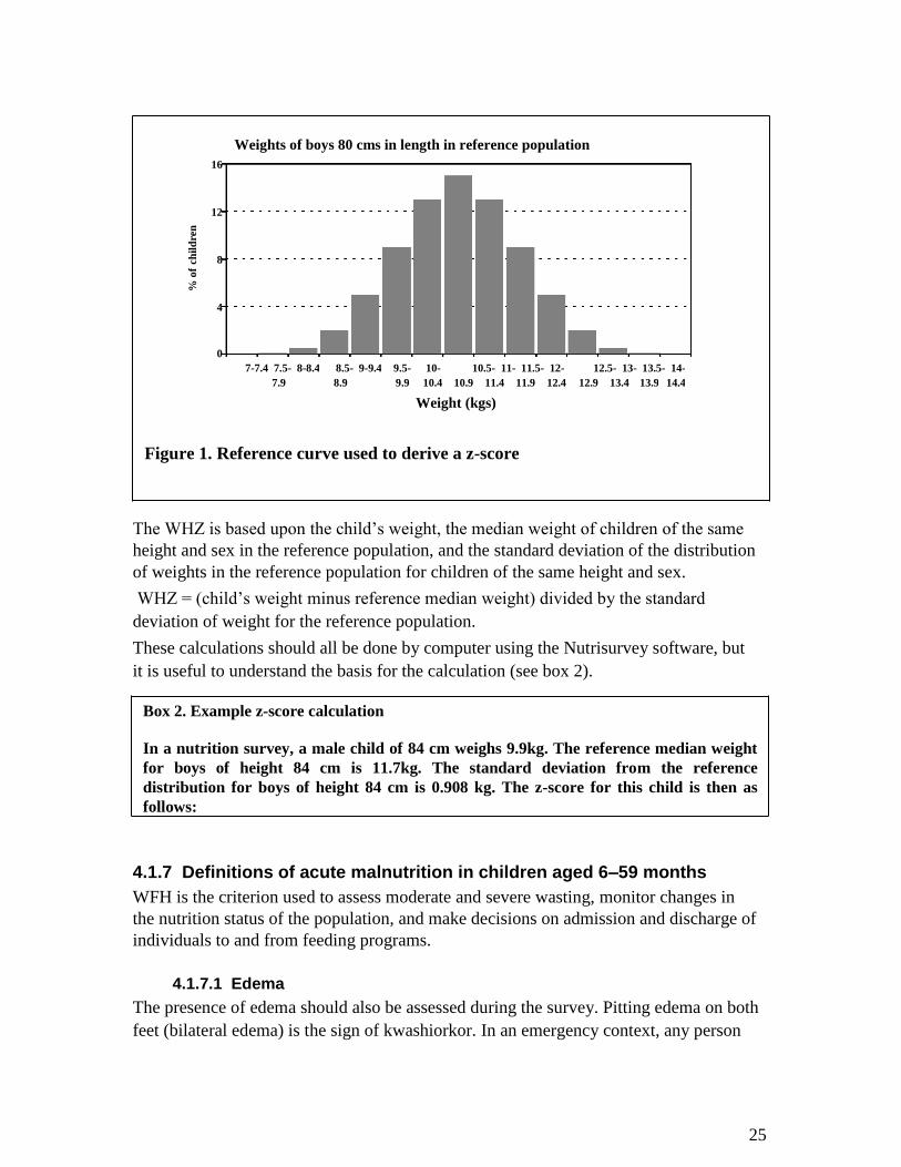
The WHZ is based upon the child’s weight, the median weight of children of the same

height and sex in the reference population, and the standard deviation of the distribution

of weights in the reference population for children of the same height and sex. WHZ = (child’s weight minus reference median weight) divided by the standard

deviation of weight for the reference population. These calculations should all be done by computer using the Nutrisurvey software, but

it is useful to understand the basis for the calculation (see box 2).

Box 2. Example z-score calculation

In a nutrition survey, a male child of 84 cm weighs 9.9kg. The reference median weight

for boys of height 84 cm is 11.7kg. The standard deviation from the reference

distribution for boys of height 84 cm is 0.908 kg. The z-score for this child is then as

follows: 4.1.7 Definitions of acute malnutrition in children aged 6–59 months WFH is the criterion used to assess moderate and severe wasting, monitor changes in

the nutrition status of the population, and make decisions on admission and discharge of

individuals to and from feeding programs.

4.1.7.1 Edema

The presence of edema should also be assessed during the survey. Pitting edema on both

feet (bilateral edema) is the sign of kwashiorkor. In an emergency context, any person

25

with bilateral edema has severe malnutrition 11

and is classified as severely

malnourished even if the WFH z-score or percent of median is normal.

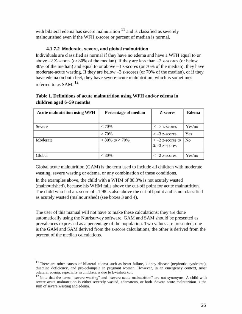
4.1.7.2 Moderate, severe, and global malnutrition

Individuals are classified as normal if they have no edema and have a WFH equal to or

above –2 Z-scores (or 80% of the median). If they are less than –2 z-scores (or below

80% of the median) and equal to or above –3 z-scores (or 70% of the median), they have

moderate-acute wasting. If they are below –3 z-scores (or 70% of the median), or if they

have edema on both feet, they have severe-acute malnutrition, which is sometimes

referred to as SAM. 12

Table 1. Definitions of acute malnutrition using WFH and/or edema in

children aged 6–59 months

Acute malnutrition using WFH Percentage of median Z-scores Edema

Severe < 70% < –3 z-scores Yes/no

> 70% > –3 z-scores Yes

Moderate < 80% to ≥ 70% < –2 z-scores to No ≥ –3 z-scores

Global < 80% < –2 z-scores Yes/no

Global acute malnutrition (GAM) is the term used to include all children with moderate

wasting, severe wasting or edema, or any combination of these conditions. In the examples above, the child with a WHM of 88.3% is not acutely wasted

(malnourished), because his WHM falls above the cut-off point for acute malnutrition.

The child who had a z-score of –1.98 is also above the cut-off point and is not classified

as acutely wasted (malnourished) (see boxes 3 and 4).

The user of this manual will not have to make these calculations: they are done

automatically using the Nutrisurvey software. GAM and SAM should be presented as

prevalences expressed as a percentage of the population. Two values are presented: one

is the GAM and SAM derived from the z-score calculations, the other is derived from the

percent of the median calculations.

11 There are other causes of bilateral edema such as heart failure, kidney disease (nephrotic syndrome), thiamine deficiency, and pre-eclampsia in pregnant women. However, in an emergency context, most bilateral edema, especially in children, is due to kwashiorkor.

12 Note that the terms “severe wasting” and “severe acute malnutrition” are not synonyms. A child with severe acute malnutrition is either severely wasted, edematous, or both. Severe acute malnutrition is the sum of severe wasting and edema.

26

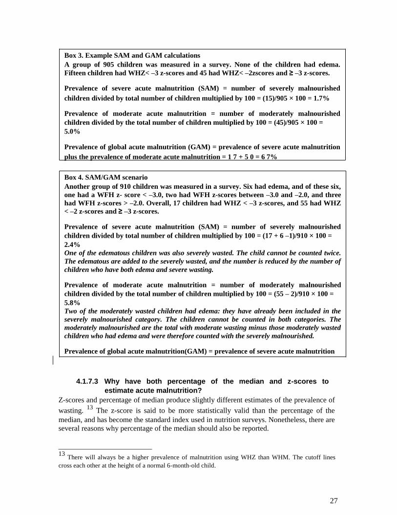
Box 3. Example SAM and GAM calculations A group of 905 children was measured in a survey. None of the children had edema.

Fifteen children had WHZ< –3 z-scores and 45 had WHZ< –2zscores and ≥ –3 z-scores.

Prevalence of severe acute malnutrition (SAM) = number of severely malnourished

children divided by total number of children multiplied by 100 = (15)/905 × 100 = 1.7%

Prevalence of moderate acute malnutrition = number of moderately malnourished

children divided by the total number of children multiplied by 100 = (45)/905 × 100 = 5.0%

Prevalence of global acute malnutrition (GAM) = prevalence of severe acute malnutrition

plus the prevalence of moderate acute malnutrition = 1 7 + 5 0 = 6 7%

Box 4. SAM/GAM scenario Another group of 910 children was measured in a survey. Six had edema, and of these six,

one had a WFH z- score < –3.0, two had WFH z-scores between –3.0 and –2.0, and three

had WFH z-scores > –2.0. Overall, 17 children had WHZ < –3 z-scores, and 55 had WHZ

< –2 z-scores and ≥ –3 z-scores.

Prevalence of severe acute malnutrition (SAM) = number of severely malnourished

children divided by total number of children multiplied by 100 = (17 + 6 –1)/910 × 100 = 2.4% One of the edematous children was also severely wasted. The child cannot be counted twice.

The edematous are added to the severely wasted, and the number is reduced by the number of

children who have both edema and severe wasting.

Prevalence of moderate acute malnutrition = number of moderately malnourished

children divided by the total number of children multiplied by 100 = (55 – 2)/910 × 100 = 5.8% Two of the moderately wasted children had edema: they have already been included in the

severely malnourished category. The children cannot be counted in both categories. The

moderately malnourished are the total with moderate wasting minus those moderately wasted

children who had edema and were therefore counted with the severely malnourished.

Prevalence of global acute malnutrition(GAM) = prevalence of severe acute malnutrition

4.1.7.3 Why have both percentage of the median and z-scores to

estimate acute malnutrition?

Z-scores and percentage of median produce slightly different estimates of the prevalence of

wasting. 13

The z-score is said to be more statistically valid than the percentage of the

median, and has become the standard index used in nutrition surveys. Nonetheless, there are

several reasons why percentage of the median should also be reported.

13

There will always be a higher prevalence of malnutrition using WHZ than WHM. The cutoff lines

cross each other at the height of a normal 6-month-old child. 27

• It is a better predictor of mortality (the outcome of dominant interest) than z-

score.

• It is used for the admission of patients to feeding programs, because it is a better

predictor of death and directs resources where they are most efficiently used.14

It is used for the admission of adolescents where WHZ cannot be used.

• It is easier for lay people to understand and for survey managers to explain

because it does not require an understanding of statistical concepts.

• It is easier to calculate with a simple calculator. Nutritional surveys should always report the prevalence of edema and of wasting (WFH)

in terms of both z-score and percentage of the median in the body of the report, as well

as the SAM and GAM.

4.1.7.4 Chronic malnutrition in children

The long time scale over which HFA changes makes it less useful for deciding when to

intervene in an emergency. It is useful, however, for long-term planning and policy

development. Although at an individual level stunting develops slowly, the degree of

stunting can change within a few months when averaged over an entire population.

Incorrect age data makes HFA information misleading, and reliable age data can be

difficult and time-consuming to obtain. For this reason, age data are generally gathered

in an emergency survey to determine if the child is appropriately included in the sample

(i.e., is the child probably between 6 and 59 months?) or whether the sample is biased

toward a particular age group, rather than to obtain accurate information about stunting.

4.2 The mortality component 4.2.1 Why do a mortality survey? Usually, public health workers at the start of an emergency have to rely on cross-

sectional surveys to determine current nutrition status and death rates in the recent past.

Ideally, surveys complement a functioning surveillance system to estimate acute

malnutrition, verify surveillance data, and answer specific questions the surveillance

system is not providing answers for or about areas that the surveillance system is not

covering. An elevated death rate can indicate that there is a health problem in a population, but it

cannot indicate the cause. 14

The nutritional status of adolescents can also be expressed as WHM, but not as WHZ. Using WHZ for

admission leads to many more admissions than WHM; the additional admissions generally do not need to be in therapeutic feeding programs.

28

4.2.2 Population for mortality surveys: all members living in the

household for at least some part of the recall period To determine the death rates, a member of each selected household is interviewed

to obtain information on deaths and in-migration and out-migration of all household

members present for at least some part of the recall period. Data required are the number of people who live in the household and the number of

deaths that have occurred during the recall period (a specified period of time in the recent

past). Each day, each member of the household is at risk of death, although very few

actually die on any given day. The actual deaths are expressed in relation to the number

of people and the length of time they were at risk. We need to find out how many people

have been at risk during the recall period—not just those in the house at the time of the

survey. Therefore household members who have left the household should be counted.

Similarly, those who have joined the household during the recall period have not been at

risk for the whole of the recall period. During the calculations, these factors are taken into

consideration.

4.2.3 Mortality measurements and indices

The crude death rate (CDR) 15

is defined as the number of people in the total population

who die over a specified period of time. It is calculated using the following formula:

Number of deaths

CDR =

(

Total population ) x Time interval = Deaths/10,000/day

10, 000

In the formula, total population is the population present at the midpoint of the time

interval. The time interval is the length of time within which the respondents are asked to

state if any deaths have occurred; this is usually referred to as the “recall period.” The units for the formula are deaths per 10,000 per day when the “time interval” is expressed

in days. 16

15 The term crude mortality rate (CMR) has been used when referring to deaths/10,000/day by some epidemiologists and those working in complex emergencies. Crude death rate (CDR) is usually used when referring to deaths/1,000/year (the units used by demographers and most epidemiologists). The terms are interchangeable. It is recommended that the term crude death rate be used. This is to maintain consistency with the expression of age-specific death rates, where there has been considerable confusion.

16 The CDR can also be expressed using other units such as deaths/1,000/month, in which case the time interval is

expressed in months and 1,000 is substituted for 10,000 in the formula. The conversion factor is 30.4/10 = 3.04 (there

are an average of 30.4 days in one month) to convert a result expressed as deaths/10,000/day to deaths/1000/month

multiply by 3.04. Similarly, to express the result as deaths/1,000/year, the time interval is expressed in years. The

conversion factor is 365/10 = 36.5. to convert death/10,000/day to death/1,000/year multiply by 36.5. The different

ways of expressing the CDR are exactly equivalent: one can be readily converted to another. In this manual and reports

it is recommended that all death rates be expressed as deaths/10,000/day to avoid confusing nonexpert readers who

become used to working with one set of units. This recommendation applies no matter the length of the recall period

used.

29

4.2.4 Nomenclature: “age-specific death rate for children less than 5,”

“under-5 mortality rate,” or “0–5 death rate” There is an important problem with nomenclature that has led to considerable confusion.

The term “under-5 mortality rate” is being used in two distinct and quite different ways. First, demographers and epidemiologists use the term to denote the calculated probability of

dying before age 5 expressed per 1,000 live births. In this original sense, it represents the

probability of a child born during a particular year dying before that child reaches 5 years of

age, assuming there is no change in the mortality rate. It is thus comparable to the infant

mortality rate, which is the probability of a live born child dying before the age of 1 year.

The calculations are quite complex, and it is also necessary to determine the birth rate. The

under-5 mortality rate, used in this sense, cannot be calculated from the survey methods

outlined in this manual. Therefore, the manual does not use the term “under-5 mortality

rate,” except in very limited circumstances. Second, those working in complex emergencies later used the same term to refer to the rate of death of children aged 0–5 over a specific time interval. It estimates the incidence of death over a recall period. In this sense it is comparable to the CDR. Epidemiologists and demographers also calculate this rate, but they refer to it as the “age-specific death

rate for children 0–5” and use the notation “5M0.” In a similar way, other age-specific

death rates can be estimated for other age ranges of the population. Although the same phenomenon is being estimated with both meanings of the term, the

concepts, calculations, and numerical results are quite different. The numerical result

using the first definition is (very roughly) five times higher than the second (although one

cannot be calculated from the other). In this manual we will restrict the term “under-5 mortality rate” to the first, original

definition. We will use the term “0–5 year death rate” (0–5DR) for the second

definition, denoting the age-specific death rate of children less than 5 years of age. This

is simply a clarification of nomenclature introduced to avoid confusion. 0–5DR is the

same as the under-5 mortality rate used in the past by those working in complex

emergencies. To be consistent, we will also use the term “crude death rate” (CDR),

rather than “crude mortality rate” (CMR), to denote the total death rate in the population

over a given time interval.

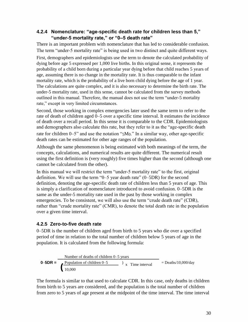
4.2.5 Zero-to-five death rate 0–5DR is the number of children aged from birth to 5 years who die over a specified

period of time in relation to the total number of children below 5 years of age in the

population. It is calculated from the following formula:

Number of deaths of children 0–5 years

0–5DR =

(

Population of children 0–5 ) x Time interval = Deaths/10,000/day

10,000

The formula is similar to that used to calculate CDR. In this case, only deaths in children

from birth to 5 years are considered, and the population is the total number of children

from zero to 5 years of age present at the midpoint of the time interval. The time interval

30

is the length of time within which the respondents are asked to state if any deaths in

children have occurred. In general the 0–5DR, is about twice the CDR.

4.2.6 Determining the recall period The recall period for the mortality survey is the time interval over which you count deaths.

Deaths that occurred before the recall period are not recorded as deaths, even though the

interviewer is often told about such deaths and will respond sympathetically. If the recall period is three months, you will try to establish the number of deaths that

occurred among your sample population during the three months prior to the day of the

survey. The number of deaths is expressed in relation to both the number of people sampled and

the number of days they have been at risk. This “person-days” at risk is the denominator

in the calculation of mortality rate. The length of the recall period is thus a critical factor

in determining the mortality rate. Six thousand people at risk over three months is mathematically equivalent, in terms of

the total risk of death, to 3,000 people at risk over six months and 18,000 people at risk

for one month. There must be a substantial number of person-days included to record

sufficient deaths and determine the mortality rate with a narrow confidence interval. If

the recall period is too short, a very large number of households will need to be visited

and interviewed, which makes the survey unwieldy. On the other hand if the recall period

is too long, the information on mortality rate may well be too out of date to be helpful in

an emergency situation, particularly if the emergency is evolving rapidly. The following

factors should be considered when you choose a recall period:

• Objectives: How will the mortality information be used? How current does the

information have to be? What time period is needed to address the objectives?

• Are mortality rates changing rapidly? If so, knowing the mortality rate over

the last few months is likely to be more important than knowing the rate over

six months or one year.

• Seasonality: Does the mortality change markedly with the different seasons? If

so then you are more likely to capture the current season if the recall period is not

longer than a few months.

• Migration: Over a short recall period, there will be fewer household members

leaving the household and fewer new members joining. This simplifies the

interview and calculations. With mass displacement there may be very few

households that have had a stable composition during a prolonged recall period.

• Accuracy: The shorter the recall period, the more accurate the estimate of

mortality. This is because more distant events are more likely to be forgotten by

respondents and there are likely to be more mistakes in the time of death. (Recall

periods longer than one year should not be used.) 31

• Precision: The longer the recall period the more precise the estimate of mortality

(the narrower the confidence interval) with a given sample size. This is because

the “sample” is actually the number of person-days considered rather than simply

the number of people. With a longer recall period, a smaller number of

households needs to be interviewed to achieve an acceptable confidence interval.

• Logistics: The longer the recall period, the fewer persons (and households)

needed in the sample. Although a longer recall period may increase the time

needed at each household, the time saved by going to fewer households more than

compensates for a longer interview. If you want to increase precision, you may increase either the length of the recall period,

the sample size (i.e., the number of households 17

in the survey), or both. Logistical

constraints usually limit the number of households that can be visited by survey teams.

4.2.6.1 How to decide on the length of the recall period

• During an acute emergency, it is usually advisable to use approximately a three

month recall period. A three month recall period is a compromise: it allows an

estimate of the death rate that is generally close enough to the current situation to

allow for planning health and nutrition interventions, while usually giving a

reasonable level of precision from about the same number of households that

will need to be visited for the nutrition component of the survey. A shorter recall

period may result in insufficient precision; a longer recall period may not be

sufficiently representative of the current situation and may increase recall bias.

• If the objective of the survey is to document mortality over a longer period of

time, recall periods of up to 12 months are justified. For example, if major

violence resulted in population displacement six months ago, you may want to

document the mortality rate for two separate periods: three or six months before,

and the six months since, the displacement. Because this increases the complexity

of the mortality survey, it should only be included if the added information is

useful and if the persons interviewed can reliably place deaths into the time

intervals. Box 5 indicates the advantages and disadvantages of lengthening the

recall period beyond three months.

17

Household definitions are culturally specific and need to be decided and agreed before the survey. A

frequently used definition is “who slept here last night and ate from the same cooking pot.”

32

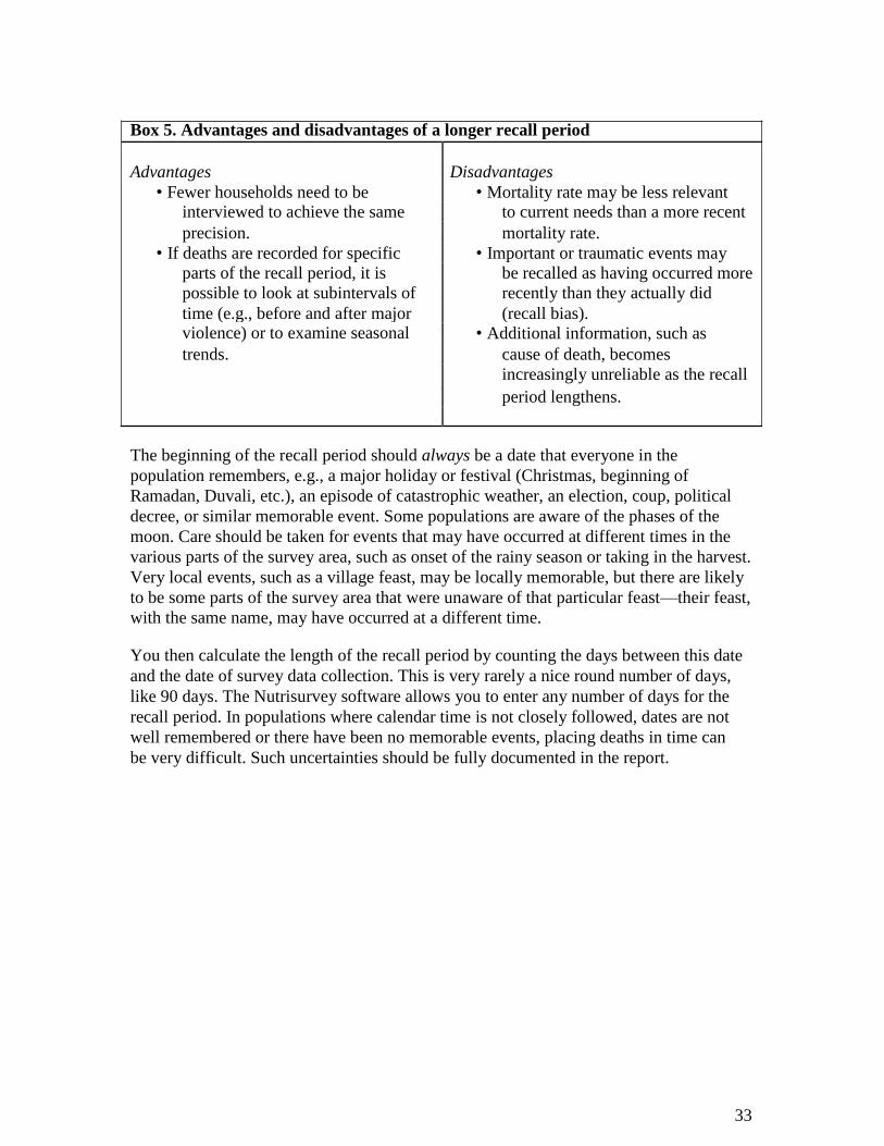
Box 5. Advantages and disadvantages of a longer recall period

Advantages Disadvantages

• Fewer households need to be • Mortality rate may be less relevant interviewed to achieve the same to current needs than a more recent

precision. mortality rate.

• If deaths are recorded for specific • Important or traumatic events may

parts of the recall period, it is be recalled as having occurred more

possible to look at subintervals of recently than they actually did

time (e.g., before and after major (recall bias). violence) or to examine seasonal • Additional information, such as

trends. cause of death, becomes

increasingly unreliable as the recall

period lengthens.

The beginning of the recall period should always be a date that everyone in the

population remembers, e.g., a major holiday or festival (Christmas, beginning of

Ramadan, Duvali, etc.), an episode of catastrophic weather, an election, coup, political

decree, or similar memorable event. Some populations are aware of the phases of the

moon. Care should be taken for events that may have occurred at different times in the

various parts of the survey area, such as onset of the rainy season or taking in the harvest.

Very local events, such as a village feast, may be locally memorable, but there are likely

to be some parts of the survey area that were unaware of that particular feast—their feast,

with the same name, may have occurred at a different time. You then calculate the length of the recall period by counting the days between this date

and the date of survey data collection. This is very rarely a nice round number of days,

like 90 days. The Nutrisurvey software allows you to enter any number of days for the

recall period. In populations where calendar time is not closely followed, dates are not

well remembered or there have been no memorable events, placing deaths in time can

be very difficult. Such uncertainties should be fully documented in the report.

33

Box 6 takes you through an example of some of the things you will have to consider in

selecting a recall period. Box 6. Example of selecting a recall period Imagine that you need to assess mortality in a rural population because it has been predicted that

next year’s harvest is going to be a failure and you want a baseline measurement now. The

seasonal calendar of events that has a direct impact on mortality is shown below. The

population faces seasonal shortages of food from May to October, but particularly from August

to October. Outbreaks of malaria occur in the season of heavy rains in January and February.

The harvest is normally due in November.

Food shortage Malaria outbreak

Jan X

Feb X

Mar

Apr

May X

Jun X

Jul X

Aug XX

Sep XX

Oct XX

Nov

Dec Imagine you undertake the mortality assessment in October. If you use a recall period of three

months, you will obtain mortality data that is affected by the worst of this year’s food shortage

period. If you use a recall period of six months, you will obtain mortality data that is affected by

the moderate food shortage as well as the more severe food shortage. Other things being equal,

your estimate of the CDR using the shorter recall period will probably give a higher CDR than

the estimate using the longer recall period, because recent mortality has probably been higher

than mortality in the more distant past. The same would be true if you were estimating the death

rate for the malaria season during an assessment in March. If you took too long a recall period,

you would dilute the effect of malaria on mortality rates. For a baseline, you may wish to select a

recall period that covers the whole previous year to include all the seasonal influences on the

mortality rate.

34

4.3 Planning the survey 4.3.1 Overview of sampling methods The sampling method is selected based upon the way in which the households

are distributed and the size of the population to be surveyed.

1. Occasionally, with very small populations, every household in the population

can be visited (an exhaustive survey), but this is unusual.

2. Where the houses of the whole population of interest are arranged in a systematic

way (such as in some refugee camps), simple or systematic random sampling is

used for the entire sampling process.

3. Cluster sampling, the most common method, is used when households are

distributed in an unstructured way that does not easily allow all households to be

listed or numbered. Normally, highly insecure areas are excluded from the population under consideration

before selecting the clusters. Sometimes extra clusters are chosen so that if one or

more cannot be visited because of sudden insecurity or refusal by leaders/elders of a

given cluster for the members to be interviewed, the clusters can be replaced. Clusters

that could not be visited cannot be considered part of the sampled population, and this

must be reported and shown on the map.

4.3.1.1 Exhaustive surveys

If all the households from a given population were interviewed and all the children

aged 6–59 months measured, we would get a precise picture of the nutrition status and

mortality rate of the population. This is called an exhaustive survey, and it is possible in

small populations such as a small camp or an institution such as an orphanage (box 7).

For a larger population, an exhaustive survey is long, costly, difficult, and unnecessary.

The results cannot be extrapolated to another camp or population. Exhaustive surveys

will not be considered further in this manual.

Box 7. Example scenario for an exhaustive survey An organization wants to know the rate of malnutrition in a small refugee camp for

which it is responsible. There are between 2,000 and 3,000 people in the camp. It is

estimated that 20% of the population is less than 5 years of age; therefore, there are

about 400–600 children less than 5 years of age. In this case, all the children were

measured and households interviewed in an exhaustive survey.

4.3.1.2 Representative sampling

Instead of interviewing all the households and measuring all the children, a sample

may be taken to “represent” the whole population. It is important that the sample be

chosen that indeed is representative of the whole population. This is done by choosing 35

households at random. The critical point is that each household and child in the

population must have an exactly equal chance 18

of being selected into the sample.

4.3.1.3 Convenience sampling is never used in a survey

Series of children measured in health centers, markets, or other places where people

gather are not representative. Children that visit health centers are not the same as those

that do not. Well children can go to the market, run around the village, and follow the

assessment team, while sick children are more likely to be in the house. The results of

measuring such groups should never be called a survey (it can be called a series), and no

decisions should ever be based upon such a “grab” sample. Similarly, clusters can never

be selected on the basis of convenience. If we were only to select households in villages

that are near to the road, the survey would be biased. Villages near roads have better

access to transport and may be wealthier than more remote villages. In each of these

examples, all the households and children in the community do not have an equal chance

of being selected. Merely going to a clinic, running around the village, or living near a

road or in the center of a village should not make anyone more likely to be selected.

4.3.2 The relationship among precision, bias, and sample size

4.3.2.1 Precision and sampling error

Most surveys that estimate the prevalence of malnutrition or death rates randomly sample

households selected from the population of concern. There will always be some

differences between the results obtained from the sample, regardless of how big it is, and

the entire population from which the sample was selected. For example, if a room

contains 10 men and 10 women, random samples of 6 persons from this room will

sometimes contain 3 men and 3 women, sometimes 4 men and 2 women, sometimes 2

men and 4 women, or, more uncommonly, 1 man and 5 women or 5 men and 1 woman;

even more rarely would the sample have 6 men or 6 women. The frequency with which

any of these samples are likely to be chosen can easily be calculated mathematically

using standard statistical theory. The same principle applies to much larger samples from

a population. Samples that are very different from the entire population are much less likely to be

randomly selected than samples that are similar to the entire population. The difference

between the value derived from a sample and the true value in the entire population is

called the sampling error. The size of the sampling error of a survey can be estimated and is presented as

confidence intervals. 19

If a survey were repeated many times with the same sample size

and method, 95% of the calculated death or malnutrition prevalence rates would fall within the 95% confidence interval. The 95% confidence interval is thus an expression of how certain we are that the actual result in the population is similar to the result we have obtained from the survey. For example, if a survey estimates the prevalence of

18

Or, if the chances are not exactly equal, the relative chances of being selected must be known

beforehand. However, this makes subsequent calculations very complicated, so for practical purposes each child must have an equal chance of being selected. 19

Other ways of expressing the sampling error, such as the standard error, are used in other contexts.

36

malnutrition to be 8.7% with a 95% confidence interval of 7.1%–9.5%, then we are

95% sure that the actual malnutrition prevalence in the population in which the survey

was done lies between 7.1% and 9.5%. 20

The confidence interval is an estimate of precision of the result, that is, how similar the

results would be if the survey were repeated over and over. If the confidence interval is

wide, sampling error may be responsible for a substantial difference between the estimate

of the death rate calculated from the survey and the true value in the population. Precision

is increased, and the confidence interval narrowed, with larger sample sizes. The larger

the sample size, the narrower the confidence interval and, if there is no bias, the more

certain we are that the survey result is close to the actual population value. For mortality

surveys the sample is “person-days,” and the sample size can be increased by either

increasing the number of subjects or the recall period. Statistically, a large sample size is

preferable. However, it takes more time, money, personnel, and other resources to

measure more children or ask more households about mortality. During planning we

decide the precision needed (how much uncertainty we will tolerate) and then calculate

exactly how many children or households are needed in the survey to achieve this

precision. Including additional children or households wastes resources, prolongs the

survey, delays the report, and gives a result that is unnecessarily precise. The Nutrisurvey

software calculates the sample size needed to achieve a given degree of sampling error in

the results of the survey. This software should be used routinely to calculate the sample

size instead of using the same sample size for all surveys. The factors entered into

Nutrisurvey to calculate both nutrition and mortality sample size must always be included

in the report.

4.3.2.2 Bias

Sampling error is not the only source of difference between a survey’s result and the

actual population value. Sampling error is due to the random selection of households

from the population. It cannot be eliminated, but it can be minimized by selecting a larger

sample. The degree of uncertainty is calculated by the software and presented in the

report. Bias is anything other than sampling error that causes the results of the survey to be

different from the actual population prevalence or rate. Bias cannot be calculated nor its

effect upon the result assessed. It is the main reason why surveys may not give an

accurate answer. The fact that the results are biased is usually not appreciated by those

doing the survey, it is usually not apparent from the results and its extent cannot be

judged by those reading the reports. Readers may distrust the results of a survey if the level of malnutrition or the death rates

differ from those expected. The reader will examine a survey particularly closely if the

results do not “triangulate.” For example, if the food security and mortality data do not

indicate there is a crisis when nutritional status is reported to be very poor, the reader will

suspect the nutritional data is incorrect because of bias. This uncertainty can lead to relief

being delayed or even denied by donors when it is urgently needed. Alternatively, it can

20

The units used for precision (confidence interval) in this manual are the same as those used for the

expressing the results. Thus, precision for GAM and SAM are expressed in as percentage of the population, and for CDR and 0–5DR as deaths/10,000/day.

37

lead to waste of supplies and resources if a relief operation is mounted when the situation

is thought to be much worse than it actually is. The reader must be able to rely on the

results of a survey, for there is a great deal at stake. A careful and full description of the

methods and precautions taken to minimize bias is essential to give the reader sufficient

confidence in the results to lead to action. If precautions to minimize bias are not taken,

and fully described in the report, a skeptical reader will assume a mistake has been made

and that the results can be discounted. Bias is minimized by use of good technique. This is the main reason why the supervisor

has to be experienced, adequate training is critical, and the report has to document all the

steps taken to eliminate or minimize bias.

4.3.2.2.1 Examples of bias 1. Because the foot piece of a length-board was loose, one team systematically

measured the height of each child 1 cm taller than he or she really was. Even though

weight was accurately measured, each child’s WFH z-score was lower than it should,

be and the prevalence of wasting was exaggerated. Any inaccuracy in the equipment

or measurement technique will lead to systematic bias.

2. Inaccurately taken weight and height—even when the inaccuracy is random and

evenly distributed between over- and under-measurement—results in systematic

overestimation of the prevalence of wasting. This overestimate is greater for

severe malnutrition than for moderate malnutrition, and relatively greater when

the true prevalence is low than when it is high. The effect of inaccurate

measurements is to widen the distribution curve. Because we are counting the

number of children in the tails of the distribution below the cut-off point of –2 z-

scores, any artificial widening of the distribution curve will increase the number

of children in the tails and thus increase the apparent malnutrition rate. Analysis

of many surveys has shown that this is a common and major cause of error. Its

extent can be estimated from examination of the standard deviation of the WFH,

which should always be 0.8–1.2 z-scores. If the SD is outside these limits, the

prevalence of malnutrition should be calculated from the mean value assuming a

normal distribution and an SD of 1 z-score unit (these calculations are performed

by Nutrisurvey); this is the result that should be reported. The report should make

it clear that the calculated prevalence is presented rather than the prevalence

obtained from the count of children below the cut-off point, because of probable

measurement errors.

3. Shortcuts are likely to be taken if the survey teams are required to work too hard,

if there is inadequate time allocated to rest periods and refreshments, or if the time

that can be spent in a particular household to administer the mortality

questionnaire and measure the children properly is insufficient. Shortcuts can take

many forms. The team members are usually aware that they have deviated from

the standard method, but through solidarity will not inform the supervisor. A few

common shortcuts should be watched for. First, a team may rush the interview or

the measurements. Most teams try to complete at least one cluster each day, and

they should be able to spend sufficient time in each house to complete their tasks

properly within one day. Therefore, the data may be much more accurate if there 38

are 20, rather than 30, households in each cluster. Increasing the sample size

may introduce substantial bias by provoking “shortcuts,” leading to an

inaccurate result despite the effort to achieve higher precision. Secondly, a team

may not select households at random when they reach a cluster site. They may

go to the village and take a “convenience” sample because of tiredness, heat,

hunger, or harassment, or because they have insufficient time to select the

sample correctly. This tends to be more common in rough terrain or when there

are long distances to walk. 4. Survey respondents sometimes misunderstand questions about mortality in their

households and tell survey interviewers, for example, that persons who left the

household are dead. This would lead to an overestimate of the death rate and

increase the difference between the death rates calculated from the survey results

and the actual population death rates. 5. The following are some of the sources of bias that occur particularly during

the interview.

a. Recall error: Respondents often fail to recall all deaths during a given recall

period. Infant deaths, in particular those within a short time after birth, are

particularly under-reported. Respondents may also misreport ages, dates,

and salient events.

b. “Calendar” error: Respondents may report events as happening within the

recall period when they did not (or vice versa) due to lack of clarity about

dates.

c. “Age heaping”/digit preference: Respondents may round ages to a number

ending in a 0 or 5. This is a particular problem with 0–5DR or other age-

specific death rates.

d. Sensitivity/taboos about death: In general, the death of a household member is

not a subject discussed readily with strangers. In some cultures, taboos about

death may hinder discussion if the subject is not broached with tact and

understanding.

e. Deliberate misleading: In some populations, with experience of relief

operations, some respondents may deliberately give incorrect answers in the

expectation of continuing or increased aid. This can be orchestrated by local

people with authority.

f. Mistranslation: Questionnaires may contain mistranslated key terms and

concepts (a common example is what constitutes a family vs. household).

Interpreters may misunderstand questions or mistranslate answers.

g. Interviewer error: Enumerators may ask questions or write down answers

incorrectly, skip questions, assume answers, or rush respondents in an effort to

complete the interview quickly.

h. Data entry error: In the process of data entry, answers can be miscoded or

entered incorrectly.

39

i. Analytic error: In the manipulation of any data, especially quantitative data

requiring statistical analysis, mathematical and conceptual errors can

generate faulty results or explanations.

4.3.2.2.2 Detecting and minimizing bias As bias cannot usually be calculated or corrected by the computer after data collection

is finished, it is critical to avoid bias during sampling and data collection. However, we can examine the quantitative data to see if there is likely to be some form

of systematic bias. The teams should be aware that such techniques will be applied

during the analysis to discourage their succumbing to the temptation to take shortcuts.

The Nutrisurvey software automatically carries out four tests for systematic bias:

1. A comparison of the data (WFH, edema prevalence, CDR and 0–5DR) collected

by the different teams: If any particular team has obtained data that is statistically different from the other teams, it is likely that this team’s technique has created a

systematic bias. The team differences are tested by a statistical technique called “analysis of variance” that is built into Nutrisurvey. The software will warn the

analyst if any team’s data are suspect. If this happens, and if there is time, the aberrant team’s clusters should be resampled using a different team and the new

data substituted for the aberrant data.21

If resampling is not feasible within a

reasonable time, the data should be analyzed with and without the aberrant clusters, and both results reported with a recommendation from the survey

supervisor indicating which result is likely to be more reliable. There has to be a full report of such occurrences and how they are resolved (e.g., perhaps the team’s

equipment is faulty or their training has been inadequate).

2. An examination of the distribution of WFH for each team separately: If the

standard deviation of WFH for any particular team is outside the range of 0.8–1.2

z-scores, their data should be replaced by the number of malnourished children

calculated from the mean value for that team.

3. An examination of the quantitative data for “digit preference”: As a result of

rounding by the team member (or respondent), the data may contain an excessive

number of reported height, weight, or age values ending in particular digits,

typically 0 or 5. This is done overall and for each individual team. Such rounding

by the measurer of the team usually results in an excess of 0 or 5 as the last digit.

The data obtained during training should also be examined for evidence of digit

preference.

21

If the second team gets data that is similar to the original team’s data, then there is probably a real

difference between the particular clusters assigned to that team and the remainder of the clusters. If this is

the case, the original data should be retained. The design effect will be unusually high. If the second team’s

data are very different from the original data this confirms there was a systematic bias in the work of the

first team.

40

4. A comparison of the data within clusters: Teams tend to get tired during the day,

and measurements are often taken more carefully in the morning than in the late

afternoon. The data collected from the first and second half of each cluster is

compared. If for example, there are 28 children in each cluster, and one cluster

was done by each team each day, then all children with cluster numbers 1–14 are

compared to those with cluster numbers 15–28. The final results for death rates,

WFH, and edema cases are compared, as well as counts of household members,

children, in- and out-migrants, and deaths and births. These tests can indicate the presence of some types of systematic bias and help resolve

the problem. Bias is particularly difficult to detect if all the teams have been trained to

make the same mistake. Furthermore, bias is more likely to go unnoticed in the interview

than with the quantitative measurements. It is far better to take great care to avoid bias

and to demonstrate to the teams during training the disastrous effects of bias. There are a

number of things that can be done to minimize bias:

• Carefully standardize measurement techniques. • Use standard weights and length-sticks to check the accuracy of

equipment.

• Train survey workers well. • Write clear questions to be asked of survey respondents • Back-translate all questionnaires. • Use more than one translator and compare their results when

interviewing the same households. • Carefully choose the start of a recall period. • Use local calendars. • Use the minimum sample size that gives adequate results so that the

teams are not stressed. • Provide comfortable transport and clothing for the staff. • Ensure adequate rest and refreshment periods. • Make sure that the payment to the teams is agreed upon and adequate. • Put together motivated, cohesive teams that participate fully in the daily

meetings and report any difficulties promptly and faithfully. The teams

must be trusted by the supervisor. • Apply the standard techniques mentioned in this manual.

4.4 Sampling: An in-depth discussion

4.4.1 Sampling methods There are three main sampling methods used for nutrition and mortality surveys: 1)

simple random, 2) systematic random, and 3) cluster sampling. Each uses a standard

method of selecting the subjects that is designed to eliminate bias and get a representative

sample. 41

The first step in setting up a sampling scheme is to clearly define the population for

which you need to estimate the prevalence of malnutrition. This might be the children

living in a refugee camp, several villages, a district, a region, or even a whole country. The second step is to obtain any available data on the population. This is critical, and the

best place to obtain population data for a district is usually from district government

offices or other agencies working in the area. Similarly, regional population data usually

are available from regional government offices. In refugee camps, you should be able to

get population data from the United Nations High Commission for Refugees (UNHCR)

or NGOs working in the camp. If no population data are available, for example for newly

displaced people or refugees, a rough population estimate can be made by estimating the

number of dwellings and the number of people in each dwelling. The next step is to choose the most appropriate sampling method to use. Simple random sampling: When a list of every household or individual (and if possible

the location) is available, individuals are randomly chosen from the list using a random

number table. This is an uncommon situation and so is rarely used. Systematic random sampling: Systematic random sampling is used when there is

either a list of households or where the population is geographically concentrated and all

the dwellings are arranged in a regular geometric pattern. Such a situation may occur in

a camp where tents are pitched row after row, in blocks of flats, where streets are laid

out in a grid, or where the houses are all along the edge of a river, coast, road, or other

major feature. The first household is chosen at random. The subsequent households are

visited systematically using a “sampling interval”; this is determined by dividing the

total number of households by the number needed to give an adequate sample. Every house should have an equal chance of being chosen before the first house is

selected. This method is usually used for small-scale surveys of limited areas. This

method is also frequently used to select the households to sample within a “cluster,” as

explained below. Cluster sampling: This most common form of sampling is done in two stages. First, the whole population is divided, on paper, into smaller discrete geographical areas, such

as villages 22

whose population is known or can be estimated. Clusters are then

randomly selected from these villages with the chance of any village being selected being proportional to the size of its population. This means that each person in the

whole area has an equal chance of being selected. 23

This is called sampling with

“probability proportional to population size.” In the second stage, the individuals are chosen at random from within each cluster area or village. 22 The term “village” is used throughout the manual for convenience. It is used here to denote any area, where people live that has been given a name by the local authorities or population. This may be a traditional village, part of a town or city, subdistrict, or even a rural area bounded by geographical features such as a stream or river. When the area is named, the population knows the boundaries of the area, and the authorities either know or can estimate the population of the area.

23 Although larger villages are more likely to be selected to contain a cluster than smaller villages, individual households within the larger village are less likely to be sampled than a household from a small village. These effects balance each other so that each household in the whole population has an equal chance of being selected.

42

4.4.1.1 Population data The population data may be very inaccurate or out of date, particularly if there has been

population movement due to an emergency. As many sources of information as possible should be used to list all known villages in the area to be surveyed. If the population figures are unavailable, use local knowledge to assign a relative size to each village. The survey team, especially the enumerators, can further assist in verifying or providing population estimates—more so if they all come from the study area. A starting village, A, is used and the other villages described in terms of their relative size (X is half the size of A, Y is twice as large as A, etc.). These factors are then used to give the villages weights. Sometimes only vague descriptions are available, e.g., very big, big, medium,

small, and very small. These descriptions can also be used to weight villages 24

for

sampling proportional to population size.

4.4.1.2 Inaccessible areas

A common problem occurs when parts of the population within the sample area are not,

or cannot be, sampled. In some countries, surveys can only be conducted within a radius

from an airstrip or road. In others, there are areas that cannot be accessed because of

insecurity, impassable roads, and rivers or mountains. While the results are often

presented as representative of the whole area, it is incorrect to do so. A map showing

the accessible areas that are included in the survey should always be presented with the

report, and it should be made clear what areas are excluded. Nobody expects surveys to be done in inaccessible areas, and the surveyors will not be

criticized for omitting such areas. However, they will be criticized for claiming that they

have included areas that are, in reality, inaccessible. The report can legitimately discuss

whether inaccessible areas are likely to be better or worse off than the surveyed areas.

(Besides the inaccessible/insecure areas, deserted villages/settlements (in pastoral

communities) should also be omitted from the sampling frame).

4.4.2 Calculating sample size With any particular study design, the calculation of the sample size depends on

the following decisions:

1. How wide a confidence interval can be tolerated? This determines the minimum

precision around the estimate of malnutrition or death rate that will result in a

useful result. 2. What are the expected malnutrition prevalence and death rate? 3. What is the likely design effect (if the survey is to use cluster sampling)?

24

It is unclear what relative sizes should be given to these descriptions; for example very big = 2,500, big =

1,600, medium = 900, small = 400, very small =100; or very big = 500, big=400, medium=300, small=200,

very small=100. It is normally better to take one typical village that everyone knows and then describe the

other villages in terms of fractions or multiples of the index village.

43

4.4.2.1 How do you make these decisions? 1) How wide a confidence interval can be tolerated? The first consideration is the

minimum precision needed to meet the objectives of the survey. If a survey is done to

determine whether one third or more of the population is malnourished, or there is a

gross elevation of death rate, for example, then much less precision is needed than for a

survey designed to estimate whether there has been a change since a similar survey

conducted three months previously. The desirable precision and expected malnutrition

prevalence/death rate are interconnected. If there is a very high prevalence of acute

malnutrition—say 40%—the precision does not need to be high to enable agencies to

make appropriate decisions. At a prevalence of over 35% or so, services will be

overwhelmed, and urgent and substantial intervention will be needed. A confidence

interval of plus or minus 10% is perfectly acceptable under these circumstances. In

general, the lower the prevalence the greater the precision needed. A survey that gives a

prevalence of malnutrition of 7.5%, but with a confidence interval of 0%–15% is not

sufficiently precise to decide whether to intervene, as the confidence interval

encompasses no malnutrition at all to a substantial proportion of the population. In this

situation, such a low precision survey would be useless for making program decisions. 2) What are the expected malnutrition prevalence and death rates? The higher the

malnutrition prevalence or death rate, the lower the precision obtained with a fixed

sample size. However, as we have seen, with a high rate of malnutrition, lower precision

is perfectly acceptable. There are ways you can guess the ranges within which the

malnutrition prevalence and death rate are likely to lie. When making this assessment,

always decide upon a plausible range of values rather than a single value. “Given the

situation, the malnutrition prevalence is unlikely to be above 20% or below 10%” would

be a reasonable statement in many situations. There may be surveillance data that include

proportions of children presenting to clinics with malnutrition; a prior survey or one in an

adjacent area of the country may have estimated these outcomes; or persons who have

worked with the population since a previous survey may have a sense of whether

malnutrition or mortality has become more or less common. A more general impression

can be also obtained by asking health workers if they see many thin children. Religious

leaders should be asked how many funerals they have conducted recently, the

approximate size of their congregations, as well as whether the number of funerals has

increased or decreased recently. 3) What is the likely design effect? For calculating sample size for cluster sampling, a

correction factor accounting for heterogeneity among clusters in the population must be

used. This factor is called the “design effect.” Using cluster sampling requires a larger

sample size than for simple or systematic random sampling. This is because subjects

within the same cluster are generally more similar to each other than to members of

different clusters, which results in a decrease in precision. The imprecision of cluster

sampling is compensated for by multiplying (increasing) the sample size calculated for

a simple random sample by the design effect. Design effects can vary from 1 (if the population is homogeneous so that all the clusters

are similar to one another) to 4 or higher where some clusters are not affected and others

are severely affected. For example, if you think that malnutrition is more or less the same

throughout the population, then the design effect is probably low. In most emergencies,

44

the design effect for malnutrition is about 1.5, increasing to 2 or more in more

heterogeneous or large-scale surveys. 25

If you anticipate that crude death rate or malnutrition prevalence is quite different in

different parts of the population, the design effect may be high and a value of at least 2

should be used in the calculation. If the design effect is thought to be much greater than

2, the population is probably sufficiently heterogeneous that two separate surveys should

be conducted, each focused upon more homogeneous sections of the population. Two

cluster surveys, each with a design effect of 1.5, can be conducted with the same effort

as one survey with a design effect of 3. In emergencies where violence causes a large proportion of deaths, the violence is very

rarely evenly distributed in time or place, and the design effect can be very high (up to

10). Such high design effects require very large sample sizes if meaningful data are to

be produced. The best sources for estimates for the design effect are usually prior surveys done in the

same, adjacent, or similar populations. Design effects from prior surveys should not be

used directly to calculate sample size for a survey if there are very different numbers or

sizes of clusters, or if there is a reason to think that the heterogeneity of malnutrition or

death has changed due to the present crisis. Table 2 shows the minimum sample size calculated for various prevalence of wasting,

and the level of precision that is commonly asked for in conjunction with the anticipated

prevalence. The column showing a design effect of 1 is for use with simple random or

systematic random samples; those showing a design effect of 1.5 or 2 are for cluster

sampling. Table 2. Precision necessary at various levels of malnutrition prevalence Malnutrition Desired

prevalence precision Sample size

% +/- % Design effect = 1.0 Design effect = 1.5 Design effect = 2.0 5 2.0 456 684 912 10 2.5 553 830 1,106 15 3.0 544 816 1,088 20 5.0 246 369 492 30 7.5 143 169 287

40 10.0 92 138 184

It is usually not feasible to achieve a precision greater than 2%. It has become common

practice to use a sample size of 900 for cluster samples (30x30). In practice more than 900

children are very rarely needed in a survey. If a much larger sample size is generated by the

calculations, you are perhaps aiming for an unrealistically precise result. It is usually

possible to use fewer than 900 children, which in turn makes the logistics of the survey

much simpler and may reduce bias. Thus, we strongly recommend that the survey supervisor

use Nutrisurvey to calculate the number of children needed for each survey.

25

The decision about severe malnutrition is more complicated, because the design effect for edema is

normally greater than for moderate or severe wasting. There is insufficient information at the moment to make recommendations about the design effect for edematous malnutrition (kwashiorkor).

45

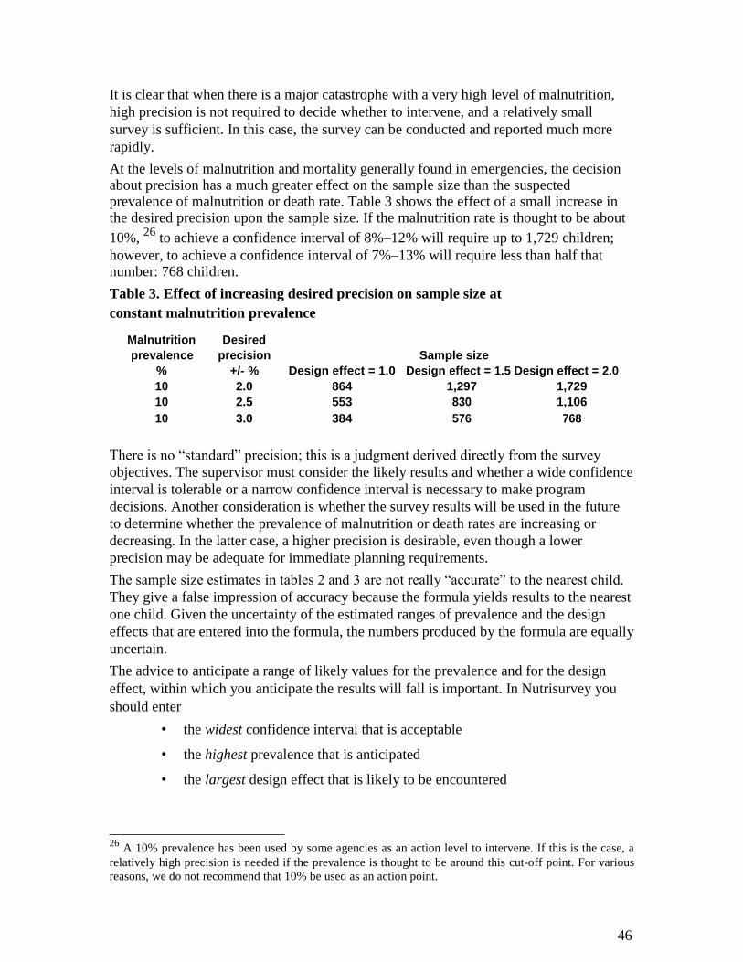
It is clear that when there is a major catastrophe with a very high level of malnutrition,

high precision is not required to decide whether to intervene, and a relatively small

survey is sufficient. In this case, the survey can be conducted and reported much more

rapidly. At the levels of malnutrition and mortality generally found in emergencies, the decision about precision has a much greater effect on the sample size than the suspected prevalence of malnutrition or death rate. Table 3 shows the effect of a small increase in the desired precision upon the sample size. If the malnutrition rate is thought to be about

10%, 26

to achieve a confidence interval of 8%–12% will require up to 1,729 children;

however, to achieve a confidence interval of 7%–13% will require less than half that number: 768 children. Table 3. Effect of increasing desired precision on sample size at

constant malnutrition prevalence

Malnutrition Desired

prevalence precision Sample size

% +/- % Design effect = 1.0 Design effect = 1.5 Design effect = 2.0 10 2.0 864 1,297 1,729 10 2.5 553 830 1,106

10 3.0 384 576 768

There is no “standard” precision; this is a judgment derived directly from the survey

objectives. The supervisor must consider the likely results and whether a wide confidence

interval is tolerable or a narrow confidence interval is necessary to make program

decisions. Another consideration is whether the survey results will be used in the future

to determine whether the prevalence of malnutrition or death rates are increasing or

decreasing. In the latter case, a higher precision is desirable, even though a lower

precision may be adequate for immediate planning requirements. The sample size estimates in tables 2 and 3 are not really “accurate” to the nearest child.

They give a false impression of accuracy because the formula yields results to the nearest

one child. Given the uncertainty of the estimated ranges of prevalence and the design

effects that are entered into the formula, the numbers produced by the formula are equally

uncertain. The advice to anticipate a range of likely values for the prevalence and for the design

effect, within which you anticipate the results will fall is important. In Nutrisurvey you

should enter

• the widest confidence interval that is acceptable

• the highest prevalence that is anticipated

• the largest design effect that is likely to be encountered 26

A 10% prevalence has been used by some agencies as an action level to intervene. If this is the case, a

relatively high precision is needed if the prevalence is thought to be around this cut-off point. For various

reasons, we do not recommend that 10% be used as an action point.

46

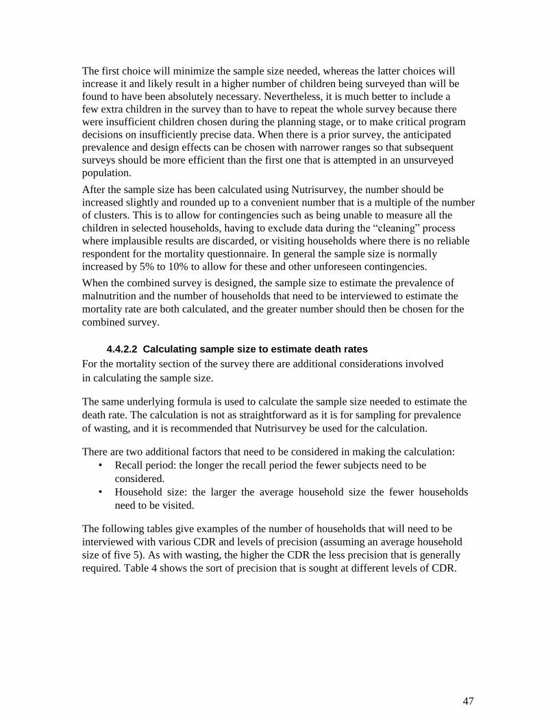
The first choice will minimize the sample size needed, whereas the latter choices will

increase it and likely result in a higher number of children being surveyed than will be

found to have been absolutely necessary. Nevertheless, it is much better to include a

few extra children in the survey than to have to repeat the whole survey because there

were insufficient children chosen during the planning stage, or to make critical program

decisions on insufficiently precise data. When there is a prior survey, the anticipated

prevalence and design effects can be chosen with narrower ranges so that subsequent

surveys should be more efficient than the first one that is attempted in an unsurveyed

population. After the sample size has been calculated using Nutrisurvey, the number should be

increased slightly and rounded up to a convenient number that is a multiple of the number

of clusters. This is to allow for contingencies such as being unable to measure all the

children in selected households, having to exclude data during the “cleaning” process

where implausible results are discarded, or visiting households where there is no reliable

respondent for the mortality questionnaire. In general the sample size is normally

increased by 5% to 10% to allow for these and other unforeseen contingencies. When the combined survey is designed, the sample size to estimate the prevalence of

malnutrition and the number of households that need to be interviewed to estimate the

mortality rate are both calculated, and the greater number should then be chosen for the

combined survey.

4.4.2.2 Calculating sample size to estimate death rates

For the mortality section of the survey there are additional considerations involved

in calculating the sample size. The same underlying formula is used to calculate the sample size needed to estimate the

death rate. The calculation is not as straightforward as it is for sampling for prevalence

of wasting, and it is recommended that Nutrisurvey be used for the calculation. There are two additional factors that need to be considered in making the calculation:

• Recall period: the longer the recall period the fewer subjects need to be

considered.

• Household size: the larger the average household size the fewer households

need to be visited. The following tables give examples of the number of households that will need to be

interviewed with various CDR and levels of precision (assuming an average household

size of five 5). As with wasting, the higher the CDR the less precision that is generally

required. Table 4 shows the sort of precision that is sought at different levels of CDR. 47

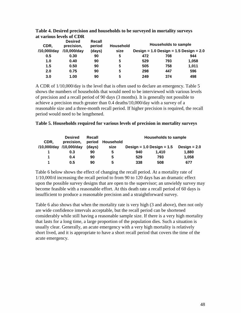
Table 4. Desired precision and households to be surveyed in mortality surveys

at various levels of CDR

CDR, Desired Recall

Households to sample

precision, period Household

/10,000/day /10,000/day (days) size Design = 1.0 Design = 1.5 Design = 2.0

0.5 0.30 90 5 472 708 944

1.0 0.40 90 5 529 793 1,058

1.5 0.50 90 5 505 758 1,011

2.0 0.75 90 5 298 447 596

3.0 1.00 90 5 249 374 498

A CDR of 1/10,000/day is the level that is often used to declare an emergency. Table 5

shows the numbers of households that would need to be interviewed with various levels

of precision and a recall period of 90 days (3 months). It is generally not possible to

achieve a precision much greater than 0.4 deaths/10,000/day with a survey of a

reasonable size and a three-month recall period. If higher precision is required, the recall

period would need to be lengthened. Table 5. Households required for various levels of precision in mortality surveys

CDR, Desired Recall Households to sample

precision, period Household

/10,000/day /10,000/day (days) size Design = 1.0 Design = 1.5 Design = 2.0

1 0.3 90 5 940 1,410 1,880

1 0.4 90 5 529 793 1,058

1 0.5 90 5 338 508 677

Table 6 below shows the effect of changing the recall period. At a mortality rate of

1/10,000/d increasing the recall period to from 90 to 120 days has an dramatic effect

upon the possible survey designs that are open to the supervisor; an unwieldy survey may

become feasible with a reasonable effort. At this death rate a recall period of 60 days is

insufficient to produce a reasonable precision and a straightforward survey. Table 6 also shows that when the mortality rate is very high (3 and above), then not only

are wide confidence intervals acceptable, but the recall period can be shortened

considerably while still having a reasonable sample size. If there is a very high mortality

that lasts for a long time, a large proportion of the population dies. Such a situation is

usually clear. Generally, an acute emergency with a very high mortality is relatively

short lived, and it is appropriate to have a short recall period that covers the time of the

acute emergency. 48

Table 6. The effect of changing recall period in mortality survey sample size

calculations

CDR, Desired Recall

Household Households to sample

precision, period

Design = 1.0 Design = 1.5 Design = 2.0

/10,000/day /10,000/day (days) size

1 0.4 60 5 796 1,193 1,591

1 0.4 90 5 529 793 1,058

1 0.4 120 5 395 593 791

3 1.0 45 5 505 758 1,011

3 1.0 60 5 377 566 754

3 1.0 90 5 249 374 498

5 2.0 30 5 315 473 631

5 2.0 45 5 209 313 417

5 2.0 60 5 155 233 311

These examples show the importance of calculating a sample size for each survey. With

the mortality survey the variables that need to be entered into Nutrisurvey are

• anticipated CDR (deaths/10,000/day)

• desired precision (deaths/10,000/day)

• recall period (days)

• household size (number of people)

• the design effect (for cluster surveys)

4.4.2.3 Sample size calculations for 0–5DR Data are normally collected for the children under 5 years old in the camp, and the 0–5

DR calculated and presented in the report. However, because the 0–5-year-olds form 15–

20% of most populations, the sample size for these children obtained from the household

interviews will be about one fifth of the sample size for the CDR. The precision around

the estimate is correspondingly poor. If a similar precision is required for the 0–5DR as

for the CDR, then it is necessary to undertake a separate mortality survey to obtain these

data specifically. The precision of the 0–5DR is not normally considered when designing

a combined nutrition/mortality survey.

4.4.3 Methods for choosing households for anthropometric and

mortality surveys In statistical terms, all sampling methods are equivalent, as long as they result in a

representative sample. The sampling scheme that should be chosen is determined mainly

by the size of the population and the physical area and organization of the households.

4.4.3.1 Simple random sampling

Simple random sampling is used where there is an up-to-date list of all individuals or

households in the population, with enough information to allow them to be located. It

is generally only used for small populations and is the most straightforward method. 49

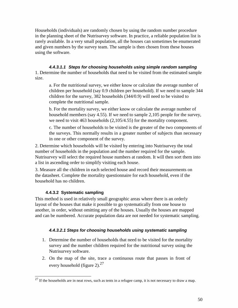
Households (individuals) are randomly chosen by using the random number procedure

in the planning sheet of the Nutrisurvey software. In practice, a reliable population list is

rarely available. In a very small population, all the houses can sometimes be enumerated

and given numbers by the survey team. The sample is then chosen from these houses

using the software.

4.4.3.1.1 Steps for choosing households using simple random sampling 1. Determine the number of households that need to be visited from the estimated sample

size.

a. For the nutritional survey, we either know or calculate the average number of

children per household (say 0.9 children per household). If we need to sample 344

children for the survey, 382 households (344/0.9) will need to be visited to

complete the nutritional sample.

b. For the mortality survey, we either know or calculate the average number of

household members (say 4.55). If we need to sample 2,105 people for the survey,

we need to visit 463 households (2,105/4.55) for the mortality component.

c. The number of households to be visited is the greater of the two components of

the surveys. This normally results in a greater number of subjects than necessary

in one or other component of the survey. 2. Determine which households will be visited by entering into Nutrisurvey the total

number of households in the population and the number required for the sample.

Nutrisurvey will select the required house numbers at random. It will then sort them into

a list in ascending order to simplify visiting each house. 3. Measure all the children in each selected house and record their measurements on

the datasheet. Complete the mortality questionnaire for each household, even if the

household has no children.

4.4.3.2 Systematic sampling

This method is used in relatively small geographic areas where there is an orderly

layout of the houses that make it possible to go systematically from one house to

another, in order, without omitting any of the houses. Usually the houses are mapped

and can be numbered. Accurate population data are not needed for systematic sampling.

4.4.3.2.1 Steps for choosing households using systematic sampling

1. Determine the number of households that need to be visited for the mortality

survey and the number children required for the nutritional survey using the

Nutrisurvey software.

2. On the map of the site, trace a continuous route that passes in front of

every household (figure 2).27

27

If the households are in neat rows, such as tents in a refugee camp, it is not necessary to draw a map.

50

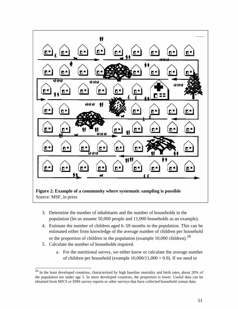
Figure 2. Example of a community where systematic sampling is possible Source: MSF, in press

3. Determine the number of inhabitants and the number of households in the

population (let us assume 50,000 people and 11,000 households as an example).

4. Estimate the number of children aged 6–59 months in the population. This can be

estimated either from knowledge of the average number of children per household

or the proportion of children in the population (example 10,000 children).28

5. Calculate the number of households required.

a. For the nutritional survey, we either know or calculate the average number

of children per household (example 10,000/11,000 = 0.9). If we need to 28

In the least developed countries, characterized by high baseline mortality and birth rates, about 20% of

the population are under age 5. In more developed countries, the proportion is lower. Useful data can be

obtained from MICS or DHS survey reports or other surveys that have collected household census data.

51

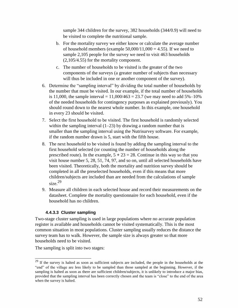
sample 344 children for the survey, 382 households (344/0.9) will need to

be visited to complete the nutritional sample.

b. For the mortality survey we either know or calculate the average number

of household members (example 50,000/11,000 = 4.55). If we need to

sample 2,105 people for the survey we need to visit 463 households

(2,105/4.55) for the mortality component.

c. The number of households to be visited is the greater of the two

components of the surveys (a greater number of subjects than necessary

will thus be included in one or another component of the survey).

6. Determine the “sampling interval” by dividing the total number of households by

the number that must be visited. In our example, if the total number of households

is 11,000, the sample interval = 11,000/463 = 23.7 (we may need to add 5%–10%

of the needed households for contingency purposes as explained previously). You

should round down to the nearest whole number. In this example, one household

in every 23 should be visited.

7. Select the first household to be visited. The first household is randomly selected

within the sampling interval (1–23) by drawing a random number that is

smaller than the sampling interval using the Nutrisurvey software. For example,

if the random number drawn is 5, start with the fifth house.

8. The next household to be visited is found by adding the sampling interval to the

first household selected (or counting the number of households along the

prescribed route). In the example, 5 + 23 = 28. Continue in this way so that you

visit house number 5, 28, 51, 74, 97, and so on, until all selected households have

been visited. Theoretically, both the mortality and nutrition survey should be

completed in all the preselected households, even if this means that more

children/subjects are included than are needed from the calculations of sample

size.29

9. Measure all children in each selected house and record their measurements on the

datasheet. Complete the mortality questionnaire for each household, even if the

household has no children.

4.4.3.3 Cluster sampling

Two-stage cluster sampling is used in large populations where no accurate population

register is available and households cannot be visited systematically. This is the most

common situation in most populations. Cluster sampling usually reduces the distance the

survey team has to walk. However, the sample size is always greater so that more

households need to be visited. The sampling is split into two stages: 29

If the survey is halted as soon as sufficient subjects are included, the people in the households at the

“end” of the village are less likely to be sampled than those sampled at the beginning. However, if the

sampling is halted as soon as there are sufficient children/subjects, it is unlikely to introduce a major bias,

provided that the sampling interval has been correctly chosen and the team is “close” to the end of the area

when the survey is halted.

52

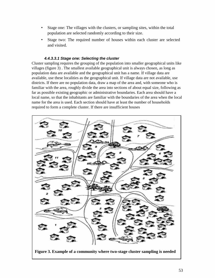
• Stage one: The villages with the clusters, or sampling sites, within the total

population are selected randomly according to their size.

• Stage two: The required number of houses within each cluster are selected

and visited.

4.4.3.3.1 Stage one: Selecting the cluster Cluster sampling requires the grouping of the population into smaller geographical units like

villages (figure 3) . The smallest available geographical unit is always chosen, as long as

population data are available and the geographical unit has a name. If village data are

available, use these localities as the geographical unit. If village data are not available, use

districts. If there are no population data, draw a map of the area and, with someone who is

familiar with the area, roughly divide the area into sections of about equal size, following as

far as possible existing geographic or administrative boundaries. Each area should have a

local name, so that the inhabitants are familiar with the boundaries of the area when the local

name for the area is used. Each section should have at least the number of households

required to form a complete cluster. If there are insufficient houses

Figure 3. Example of a community where two-stage cluster sampling is needed

53

in a village, two adjacent villages should be combined at the planning stage. The selection of the sections (from which a cluster will ultimately be chosen) must be

conducted so that the chance of any particular section being selected is proportional to the

population of the section. Thus, if one section has a population of 5,000 and another

1,000, then the first section has five times the chance of being chosen to contain a cluster.

This is the main reason why (approximate) population data are required. Steps in choosing the clusters: 1. Determine the sample size using Nutrisurvey. 2. Obtain the best available census data for each village, district, or section on the map.

This is usually obtained from the local government offices. In a stable population, such

as a drought-affected region with little in- and out-migration, a census that is several

years old may still be acceptable as a base for population proportionate sampling.

However, in refugee situations where influx continues, reliable up-to-date counts are

important for a valid sample. Alternatively, if no population data are available, estimate

the relative size of the population living in each section of the map using a key informant. 3. On the planning page of Nutrisurvey (right-hand side of pane) there is a table. Enter

the names of all the villages (districts or sections on map) into the left column and

their population size into the right-hand column. The order you enter the villages is not

important, but it is important that they all be included. The Software will automatically select the villages that should contain a cluster. You will not be able to change a cluster site once it is selected. If the survey is to be

unbiased, the selected site must be visited. Thus, it is important to define your

geographical area in the planning stage very realistically, taking travel, security, and any

other factor that could influence your ability to get to the cluster site into account before

listing the sites in the planning table. Large villages or sections of towns may be selected for more than one cluster. If this

happens, the village should be divided in two equal sections geographically (say north

and south) and one cluster taken at random from each division.

4.4.3.3.2 How many clusters should be selected? The number of children in a cluster should generally be chosen so that one team can

complete one cluster per day. If it is anticipated that the teams can only measure, say, 20

children per day, then the best strategy is to increase the number of clusters. The design

effect is smaller with a larger numbers of clusters, meaning that although there may be

more clusters, fewer total numbers of children are likely to be needed. Thus, sampling

40 or 45 clusters of 20 children is more efficient than 30 clusters of 30 children. If the teams leave base at 8 am, take one hour to reach the cluster site and another hour

to introduce themselves and select the first house, then measurements will start at 10am.

The team will need two refreshment breaks of 15 minutes each, one hour for lunch, and

54

will need to leave to get back to base before dark, say about 4pm. 30

This means that the

team will have 4.5 hours to measure children and interview household heads. If 30

households are to be visited, there will be about 7 minutes for each child and interview,

with 2 minutes to reach the next house and introduce the team to the new house. Thus, all

the data that is to be gathered from a family should be able to be collected in about 7

minutes. If there are 20 visits to be made in the same time then the team can spend 11.5

minutes at each house. With only 15 visits per cluster, the team could spend 16 minuets at

each house. These practical points should be considered when designing the survey. If the

distances between houses are not great and there is no insecurity, more children can be

included in a cluster. This is one reason why sample size should always be calculated to

have the minimum number of visits that is compatible with the desired survey precision. In households where the mother is not the respondent for the mortality interview, it is

possible to conduct the interview and make the measurements on the children

simultaneously (if there are separate team members for interviewing and measuring).

However, in most households the mother will need to be interviewed. She should also be

with her children when they are measured if they are not to be frightened by the team (of

strangers). Thus, the two components of the survey will often need to take place

consecutively even if there are additional team members. (The interview should always

take place before the anthropometric measurements. During the interview, the children

will “settle down,” see that the mother interacts with the team harmoniously and be more

amenable to being measured). Some houses will have to be revisited at the end of the day to measure children that were

missing during the first visit. If the time scale simply cannot be kept, there are two

choices. The team could use two days to measure one cluster, which will double the time

taken to collect the data. This is undesirable. Alternatively the number of children in each

cluster can be reduced and the total number of clusters increased, affording more time to

carefully collect data. This is a far better option. Thus, if data from 30 children, for example, cannot be collected in one day during the

field test at the end of the training session, the number of clusters should be increased and

the number of children in each cluster correspondingly reduced. The commonly used 30 by 30 cluster survey design is calculated to cover nearly every

situation and give a relatively high precision when there is a high prevalence of

malnutrition. It is designed to accommodate “worst case” situations, ensuring that nearly

all surveys will have sufficient children regardless of the experience of the surveyor. In

general it is found that most surveys could have been adequately conducted, more

cheaply and rapidly, with fewer children. To avoid “shortcut” bias, it is better to measure

fewer children accurately than overstress the team so that the measurements are not

made accurately (see example in Box 8). You should always plan to have at least 30 clusters. As the number of clusters decreases, the

design effect increases rapidly, and fewer than 26 clusters can yield unreliable results.

30

Before leaving, the teams will need to attend the briefing meeting, check their equipment, obtain their

refreshment, fuel the vehicle, etc. Adequate rest and refreshment are essential and time must be allocated.

In emergency situations, it is inadvisable to travel after dark.

55

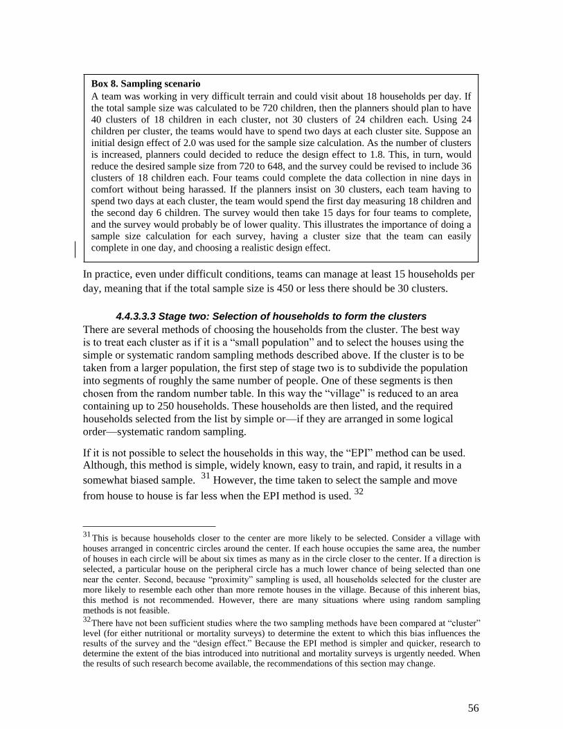
Box 8. Sampling scenario A team was working in very difficult terrain and could visit about 18 households per day. If

the total sample size was calculated to be 720 children, then the planners should plan to have

40 clusters of 18 children in each cluster, not 30 clusters of 24 children each. Using 24

children per cluster, the teams would have to spend two days at each cluster site. Suppose an

initial design effect of 2.0 was used for the sample size calculation. As the number of clusters

is increased, planners could decided to reduce the design effect to 1.8. This, in turn, would

reduce the desired sample size from 720 to 648, and the survey could be revised to include 36

clusters of 18 children each. Four teams could complete the data collection in nine days in

comfort without being harassed. If the planners insist on 30 clusters, each team having to

spend two days at each cluster, the team would spend the first day measuring 18 children and

the second day 6 children. The survey would then take 15 days for four teams to complete,

and the survey would probably be of lower quality. This illustrates the importance of doing a

sample size calculation for each survey, having a cluster size that the team can easily

complete in one day, and choosing a realistic design effect.

In practice, even under difficult conditions, teams can manage at least 15 households per

day, meaning that if the total sample size is 450 or less there should be 30 clusters.

4.4.3.3.3 Stage two: Selection of households to form the clusters

There are several methods of choosing the households from the cluster. The best way

is to treat each cluster as if it is a “small population” and to select the houses using the

simple or systematic random sampling methods described above. If the cluster is to be

taken from a larger population, the first step of stage two is to subdivide the population

into segments of roughly the same number of people. One of these segments is then

chosen from the random number table. In this way the “village” is reduced to an area

containing up to 250 households. These households are then listed, and the required

households selected from the list by simple or—if they are arranged in some logical

order—systematic random sampling. If it is not possible to select the households in this way, the “EPI” method can be used. Although, this method is simple, widely known, easy to train, and rapid, it results in a

somewhat biased sample. 31

However, the time taken to select the sample and move

from house to house is far less when the EPI method is used. 32

31 This is because households closer to the center are more likely to be selected. Consider a village with houses arranged in concentric circles around the center. If each house occupies the same area, the number of houses in each circle will be about six times as many as in the circle closer to the center. If a direction is selected, a particular house on the peripheral circle has a much lower chance of being selected than one near the center. Second, because “proximity” sampling is used, all households selected for the cluster are more likely to resemble each other than more remote houses in the village. Because of this inherent bias, this method is not recommended. However, there are many situations where using random sampling methods is not feasible.

32 There have not been sufficient studies where the two sampling methods have been compared at “cluster” level (for either nutritional or mortality surveys) to determine the extent to which this bias influences the results of the survey and the “design effect.” Because the EPI method is simpler and quicker, research to determine the extent of the bias introduced into nutritional and mortality surveys is urgently needed. When the results of such research become available, the recommendations of this section may change.

56

4.4.3.3.4 Steps in using the EPI method When the team arrives at the village that will contain the cluster, the following

procedure should be followed after discussions with the village leaders: 1. Go to somewhere near the center of the selected cluster area. 2. Randomly choose a direction by spinning a bottle, pencil, or pen on the ground and

noting the direction it points when it stops. 3. Walk in the direction indicated, to the edge of the village. At the edge of the village

spin the bottle again until it points into the body of the village. Walk along this second

line counting each house on the way.33

4. Using a random number list select the first house 34

to be visited by drawing a random

number between 1 and the number of households counted when walking. For example, if the number of households counted was 27, then select a random number between one and

27. The team will not have a computer in the field, so each day35

before setting out, the supervisor should print out the list of random numbers. If the number 5 was chosen, go back to the fifth household counted along the walking line. This is the first house you should visit. 5. Go to the first household and examine all children aged 6–59 months in the household

for the nutritional survey and complete the mortality questionnaire. 6. The subsequent households are chosen by proximity. In a village where the houses are

closely packed together, choose the next house on the right.36

Continue in this direction

until the required number of children have been measured and subjects enumerated for the mortality survey. The same method should be used for all the clusters. If the village is spread out, choose the house with the door closest to the last house surveyed, whether on the right or left; this saves a lot of time in an area where the dwellings are spread out. Continue the process until the required number of children has been measured.

4.4.4 When the house is selected

4.4.4.1 Too many children

In cluster sampling, when the last house is visited to get the last child in a cluster, there are

often several children in the household. If so, they should all be measured and

33 As the houses closer to the center are more likely to be on the walking line from the center, this modification of the standard EPI method is suggested to reduce bias when the walk is started from the center of the village.

34 It is important to carefully define a household. It is usually defined as a group of people who regularly eat together from the same cooking pot, but those that contribute to a common economy or sleep in the same compound may be more appropriate. The definition has to be decided at the planning stage, and the same definition applied by all teams consistently. Polygamous families may constitute one or more households.

35 These can be generated and printed when planning the survey. One list is printed for each cluster and numbered 1 to 30 (or whatever the total number of clusters). The team then takes the random sheet with them when they visit the village.

36 Or left, but this should be decided during the planning stage and the same rule should be used by all the teams. It is more convenient to always go to the right for every survey.

57

included in the sample. Thus, if the planned cluster size is 25, some of the clusters

will end up with one or two more children in the cluster. This is expected. In systematic sampling, the plan for selecting houses should be followed and all the

children in the houses measured, even if this means that more children are measured

than calculated by the sample size.

4.4.4.2 Not enough children

In cluster sampling, if the team runs out of houses to measure in a village (e.g., they go to

all the houses in a village) without identifying enough children, it will be necessary to go

to the next nearest village to complete the survey. When they arrive at the next village,

the process of selecting a house at which to start is repeated. Proceed from house to house

until a sufficient number of children have been measured. In systematic sampling, if the team has finished going to all the houses planned and there

were insufficient numbers of children, the whole sampling procedure needs to be repeated to

select the remaining children. This is done by finding a new sampling interval and a new

starting point. In the example given above, if another 40 children are needed then the new

sampling interval (11,000/40) will be 275. They also need a new random starting point—say

193. They now need to visit every 275th household, starting at house 193, to find the

remaining children. This is tiresome and doubles the work to find a few extra households. It

is important not to overestimate either the proportion of children aged 6–59 months or the

average household size when calculating the sampling interval. If the sampling interval is too

large the total number of children measured will not be enough. The sampling should not end

when the predetermined number of children is found; it should continue until all the houses

that were selected are visited, even if there are additional children and subjects for the

morality survey; they form part of the sample.

4.4.4.3 No substitution

In each of the methods of selecting houses, whenever a house is selected according to the

rules, there should not be a substitution for this house for any reason. House occupants

sometimes refuse to be measured, the staff sometimes fear dogs, local people may try to

direct the team to include particular houses and omit others, or houses may be deserted or

physically difficult to reach (up a steep hill for example). If for any reason the selected

house is not included, the team must make a note and go to the next house according to

the rules. Another house is not substituted for the properly selected house. This is not

usually a problem with the EPI method, because the rules say that the nearest house to the

right should be the next selected. (In this case, however, a house to the left should not be

substituted.)

4.4.5 In the house Regardless of the sampling method, the house is the unit that is selected. Before it is

visited, it is not known how many children are in the household, or whether there are any

children at all.

58

4.4.5.1 Measure all the children All the children living in the house in the correct age range should be included in the

sample and measured. If two eligible children are found in a household, both are

included, even if they are twins. This is extremely important, as it ensures that every child

has the same chance of being selected, which is a basic principle of the survey design.

Some agencies used to select a single child to represent a household, reasoning that the

other children would have a similar nutritional status. Surprisingly, detailed analysis has

shown that there is little correlation between the nutritional status of children living in the

same household. Individuals, rather than households, seem to become malnourished.

4.4.5.2 No children

For all the sampling methods, if there are no children under age 5 in a household, the

house should remain a part of the “sample” that contributes zero children to the

nutritional part of the survey. However, it is very important to include this house for the

mortality survey. Collect the data on mortality and any other data that forms part of the

survey, record the household on the nutritional data sheet as having no eligible children,

and proceed to the next house according to the rules. On the datasheet, there is normally

one line for each child. In cluster sampling, this goes up to the number of children chosen

for the cluster plus three because the last house that is visited may have more than one

child. The next lines on the data sheet should be used to record households with no

children in them and the household is given a “household survey number.” With

systematic sampling go to the next selected house according to the plan (in the example,

if there are no children in house 23, then collect the mortality data and go to house 41, but

never to house 22 or 24. It is important that the households are recorded with an identical

identifying number on the nutritional data collection forms and the household census/

mortality forms.

4.4.5.3 Empty houses

If the house is empty, the neighbors should be asked about the family that lives in that

house. On the data collection form, record why the house is empty (if this can be

determined). If the residents are likely to return before the team leaves that cluster, the

team should return to the house to include the residents in the survey. If the house is

permanently empty or the residents will not return before the team must leave, this house

can be skipped and a note made. If the house is empty because all the members are dead,

the neighbor should be interviewed and all the residents recorded as having died. Again,

do not substitute a house that is not in the original sample for the empty house.

4.4.5.4 Absent children

If a child lives in the house but is not present at the time of the survey, this child is

recorded on the datasheet when the house is visited. Of course the weight and height

cannot be entered at that stage. Tell the mother you will come back to the house later in

the day, after you have been to all the other houses in the cluster or systematic sample.

Then go back to the house to find the child. The team should continue to look for missing

children until they leave the survey area. There are always some children who cannot be

weighed or measured, and this needs to be recorded and reported. The team should not

simply take another child and forget about the child that is missing. If more than 5% of

59

the children in a survey are not found, the teams should revisit the area at another time

to see if they can complete the sample.

4.4.5.5 Disabled children

Disabled children that would otherwise be eligible should be included where possible. If

it is not possible to measure height and weight due to deformity or other abnormality, the

child should be given an ID number and the data recorded as missing (and a note taken).

Of course, with missing height, they will not be included in the final sample unless they

have edema.

4.4.5.6 Child in a center

If a child has been admitted to a hospital or feeding center, the team must go to the center

and measure the child. This is critical, as such a child is very likely to be severely or

moderately malnourished. If it is impossible to visit the center (it may be many miles

away), the child should be included in the datasheet and a note added that the child was in

a feeding center and probably severely malnourished. In reality, the child may or may not

be severely malnourished. If there are a large number of such children, and the centers

cannot be visited to complete the measurements, then two rates of severe malnutrition can

be calculated, one assuming that these children are all severely malnourished, and the

other excluding these children from the survey.

4.4.6 Problems often encountered

4.4.6.1 Population scattered over a large area

Population scattering is common in pastoral areas. The population numbers are usually

very inaccurate and it takes a longer time to travel between sites and find the subjects. If

the settlements are small it is essential to have more clusters, with fewer children per

cluster, to ensure there will be a sufficient number of children at each site. In some situations where the population is very spread out, you may deliberately choose

to undertake a survey without sampling certain sections of the population. You might

choose to sample only the population in larger settlements, which would save you the

time and money needed to get into the bush to the more scattered population. This

would mean you would not include population estimates from the scattered area when

you are originally selecting your sample. As a result, you would have no accurate data

about the nutritional status of children or the mortality rate in the population excluded

from the survey. It is critical that the reader of the report not be misled: there must be a

clear description of the exclusion in the report. The decision to exclude or include

sections of the population, such as small groups of scattered nomads whose current

whereabouts is unclear, will depend upon anecdotal reports of whether these groups are

more or less affected than those that are more easily accessible.

4.4.6.2 Population is very mobile

If you are attempting to undertake a survey in an area of nomads where the population

frequently moves large distances, it likely that you may travel to an area to find that there

is no one there or nearby. If you suspect this might happen, you should select some extra

60

clusters before you start the survey. This way, if one cluster is deserted you can replace it

with another. It is sometimes more appropriate to list the names of the nomadic groups, clans, or

extended families themselves instead of villages or other fixed settlements. The clans to

be sampled are then selected proportional to population size, and the teams set out to find

the named groups within their migratory range. However, sampling of nomads is a highly

specialized topic. Either the advice of an experienced epidemiologist should be sought, or

nomadism should be a cited as a reason for exclusion. Occasionally in nomadic areas

with a very sparse population, it is not possible to do a representative survey.

4.5 Training the teams Training the teams is one of the most important aspects of doing a survey. It should not

be rushed or assumed, as inaccurate measurements can have a very large effect upon the

prevalence of malnutrition reported by a survey. As discussed, the Nutrisurvey software

has certain checks built in to examine the internal structure of the data to see if the teams

are consistent with each other, that the measurers are not rounding the values

inappropriately, and that there are not large numbers of unlikely values. At the outset, it is

important that the team knows that and the data they collect will be analyzed in this way,

and that any shortcuts taken are likely to become apparent. However, there is no

substitution for having a well trained, confident team that makes accurate and precise

measurements. The software may recognize poorly conducted surveys, but it cannot

correct them. Team members have to understand the principles of doing a survey, the reasons why the

survey is being done, and the likely interventions that could result depending upon the

findings. They have to be comfortable with this knowledge and not confused. They have

to be able to explain and answer questions from community leaders, fathers, and mothers.

They have to be sufficiently well trained to be confident when they go into the

community. They must also learn to select the houses, talk to the mothers, make the

specific measurements, and record the results. This requires practice. Survey members will be formed into teams. It is important that team members get on well

with each other. Responsibilities, including the role of team leader, will be assigned at the

end of the training. However, each team member should be able to perform all roles. The training usually takes at least three days and should include the following:.

1. A clear explanation of the objectives of the assessment.

2. A clear explanation of roles and responsibilities of each team member, the team

leader, and the survey supervisor (they should also be given a written “job

description”).

3. An explanation of the sampling method that stresses the reasoning behind and

importance of each child and household member having an equal chance of being

selected (including households without children for the mortality survey). The

idea of random selection is sometimes difficult to grasp. Games, such as taking

counters from a bag, should be used to illustrate the principles.

4. A demonstration of weight and height measurements.

61

5. Practice taking height and weight measurements and assessing the presence of

edema. After team members have practiced taking measurements, they are

formally tested. For the tests, 10–20 children of different ages between 6 and 59

months are recruited. Each team measures each child in rotation. The teams go

round two times so that each child is measured twice by each team. The data are

entered into the computer during the training course. The software calculates how

precise (ability to get the same result on the same child each time) and how

accurate (how close the team is to “true” value, which is taken to be either the

average or the supervisor’s values) each team is in taking the measurements.

After training and practice, any team member who is unable to measure and

record the anthropometry of the children within the limits set by the computer

program should be replaced or retrained.

6. Teams should visit a therapeutic feeding center, hospital, or clinic to see cases

with edema and practice checking for edema with actual cases. Note that most

cases encountered during a survey will have mild edema, and the teams should

not be trained exclusively on cases with gross edema. It is very common for teams

to make errors in assessing edema if they have only practiced on normal children,

none of whom have edema.

7. An explanation of, and training in obtaining any additional data that need to be

collected.

8. Instruction and practice administering the mortality questionnaire. Both male- and

female-headed households should be visited. There should be at least twice the

number of households as teams. Each team visits each household and administers

the mortality questionnaire. As there is likely to be a “learning” effect by the

respondent, each team should be the first to visit two of the practice households.

The teams should get identical results.

9. A full-scale pilot test in the field. During the last day of the training, the team

visits a village that is not part of the real survey, but is similar and convenient to

the training location. The teams go through all the steps in conducting the survey,

under supervision, in that village. Data collected during the pilot test should not

be included in the survey results. During the pilot test the teams will demonstrate the following:

1. They understand and can follow the sampling procedure. This means that the

team will practice selecting the first house, the respondent(s), and children of the

right age.

2. They can take and record measurements correctly under field conditions. This

means that the team members will practice working as a team, each with his

or her allotted tasks.

3. They can administer the mortality questionnaire.

4. They can interact amicably and effectively with the respondents.

5. They have the ability to organize the transport and care of the equipment. At the end of the pilot test, the team members, leader, and survey supervisor should be

confident that each team can undertake the survey accurately, and should know how long

62

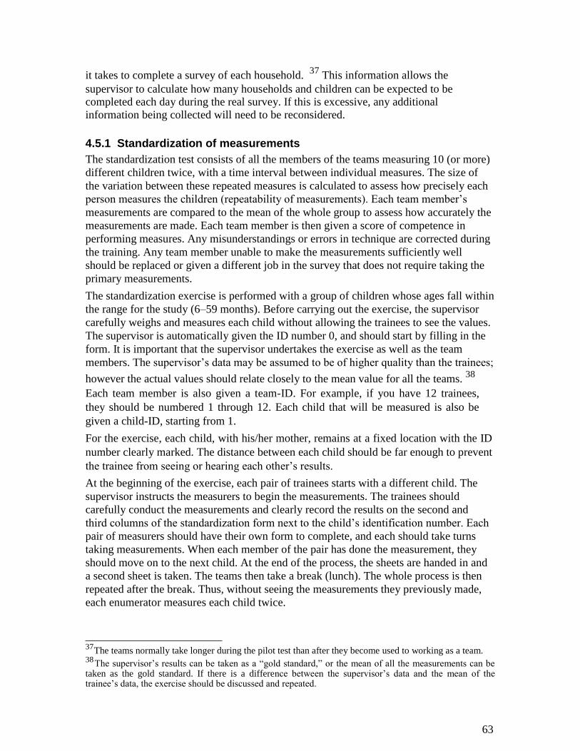
it takes to complete a survey of each household. 37

This information allows the

supervisor to calculate how many households and children can be expected to be completed each day during the real survey. If this is excessive, any additional

information being collected will need to be reconsidered.

4.5.1 Standardization of measurements The standardization test consists of all the members of the teams measuring 10 (or more)

different children twice, with a time interval between individual measures. The size of

the variation between these repeated measures is calculated to assess how precisely each

person measures the children (repeatability of measurements). Each team member’s

measurements are compared to the mean of the whole group to assess how accurately the

measurements are made. Each team member is then given a score of competence in

performing measures. Any misunderstandings or errors in technique are corrected during

the training. Any team member unable to make the measurements sufficiently well

should be replaced or given a different job in the survey that does not require taking the

primary measurements. The standardization exercise is performed with a group of children whose ages fall within

the range for the study (6–59 months). Before carrying out the exercise, the supervisor

carefully weighs and measures each child without allowing the trainees to see the values.

The supervisor is automatically given the ID number 0, and should start by filling in the

form. It is important that the supervisor undertakes the exercise as well as the team

members. The supervisor’s data may be assumed to be of higher quality than the trainees;

however the actual values should relate closely to the mean value for all the teams. 38

Each team member is also given a team-ID. For example, if you have 12 trainees,

they should be numbered 1 through 12. Each child that will be measured is also be

given a child-ID, starting from 1. For the exercise, each child, with his/her mother, remains at a fixed location with the ID

number clearly marked. The distance between each child should be far enough to prevent

the trainee from seeing or hearing each other’s results. At the beginning of the exercise, each pair of trainees starts with a different child. The

supervisor instructs the measurers to begin the measurements. The trainees should

carefully conduct the measurements and clearly record the results on the second and

third columns of the standardization form next to the child’s identification number. Each

pair of measurers should have their own form to complete, and each should take turns

taking measurements. When each member of the pair has done the measurement, they

should move on to the next child. At the end of the process, the sheets are handed in and

a second sheet is taken. The teams then take a break (lunch). The whole process is then

repeated after the break. Thus, without seeing the measurements they previously made,

each enumerator measures each child twice.

37 The teams normally take longer during the pilot test than after they become used to working as a team.

38 The supervisor’s results can be taken as a “gold standard,” or the mean of all the measurements can be taken as the gold standard. If there is a difference between the supervisor’s data and the mean of the trainee’s data, the exercise should be discussed and repeated.

63

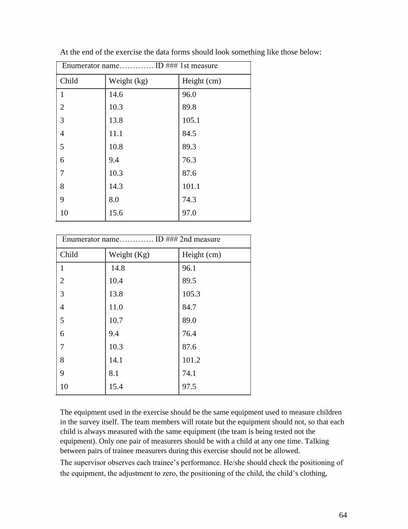
At the end of the exercise the data forms should look something like those below:

Enumerator name…………. ID ### 1st measure

Child Weight (kg) Height (cm)

1 14.6 96.0

2 10.3 89.8

3 13.8 105.1

4 11.1 84.5

5 10.8 89.3

6 9.4 76.3

7 10.3 87.6

8 14.3 101.1

9 8.0 74.3

10 15.6 97.0

Enumerator name…………. ID ### 2nd measure

Child Weight (Kg) Height (cm)

1 14.8 96.1

2 10.4 89.5

3 13.8 105.3

4 11.0 84.7

5 10.7 89.0

6 9.4 76.4

7 10.3 87.6

8 14.1 101.2

9 8.1 74.1

10 15.4 97.5

The equipment used in the exercise should be the same equipment used to measure children

in the survey itself. The team members will rotate but the equipment should not, so that each

child is always measured with the same equipment (the team is being tested not the

equipment). Only one pair of measurers should be with a child at any one time. Talking

between pairs of trainee measurers during this exercise should not be allowed.

The supervisor observes each trainee’s performance. He/she should check the positioning of

the equipment, the adjustment to zero, the positioning of the child, the child’s clothing,

64

and the angle at which the reading is taken. The supervisor should make notes on any

errors to be discussed with the team members later. The results of the training exercise are analyzed by entering the data into the

Nutrisurvey software and producing the training report. If the results are poor, the whole exercise should be repeated, perhaps with different

people paired in teams.

4.5.2 Field training Field training is practical and not confined to the classroom. It takes place after the teams

are able to make accurate and precise measurements, have “passed” the standardization

test, and have formed teams that have practiced working together. For field testing the

teams go to a convenient, local village that has not been chosen to contain a cluster.

They practice selecting the houses that will form the cluster, approaching mothers and

explaining the purpose of the survey, making the measurements, and conducting the

mortality interview. This step is essential for the teams to feel confident when they begin

conducting the actual survey. The field training data from each of the teams is entered into Nutrisurvey and analyzed.

The teams should each have selected different households from the village (otherwise it

is likely that the selection was not random) . Each team’s results will be slightly

different; this is used as a practical demonstration of the effect of sampling error and the

importance of taking a random sample.

4.6 Nutritional measurements 4.6.1 Weighing equipment The scale has to be light and robust. A suitable instrument for weighing children aged 6–

59 months is a 25kg hanging spring scale marked out in increments of 0.1kg. Weighing

pants should be provided with this scale. An electronic scale such as the Uniscale can

also be used. Bathroom scales are not sufficiently accurate.

4.6.2 Equipment for measuring height and length The measuring board should be at least 130cm long and made of hardwood with a hard water-resistant finish. Choice of wood is important; the boards should be light enough to

easily carry from house to house and should not warp in the rainy season. 39

The board

should have two tape measures attached to it, one on each side, and they should be marked out in 0.1cm increments. The foot-piece must be easily adjustable, remaining perpendicular

to the board. 40

The board should be easily set upright to measure height; the head piece of

the length board becomes the base when the board is set upright. It must be large enough for a child to stand on it and to stabilize the whole board when it is set 39 Aluminum should not be used, because it can get very hot in the sun, and aluminum has a sufficiently high specific heat to burn children. The tapes should not be of metal for the same reason. A wooden board is most comfortable for the child. Rigid plastic boards are acceptable but expensive.

40 It is best lubricated by rubbing with a candle.

65

upright. Measuring boards are usually made by local carpenters, but there should be at

least one commercial board to be used as a carpenter’s template to standardize the locally

made boards. A height arch can be used for selecting children shorter than 110cm. This

can be constructed simply and should consist of a horizontal bar fixed at 110cm above

the ground at right angles to a vertical pole (or between two vertical poles). Any child

who can walk under this horizontal bar without hitting it, and without stooping, should be

included in the sample for further measuring. All the boards are standardized with a broom handle or dowel that has been cut

to measure exactly 100cm.

4.6.3 Estimating age In many rural areas of the developing world, the age of children is not known. In general,

the younger the child is, the more accurately you can estimate the month of birth. The

following methods may be helpful if the mother does not know the child’s birthday.

1. The mother may have the child’s immunization card, road-to-health card, or other

written document showing the child’s age or date of birth. Always ask to see the

child’s immunization card.

2. If the age of a neighbor’s child is known, ask whether their child was born before

or after the selected child.

3. Use a “local-events calendar,” which shows dates on which important events

took place during the past five years. It can show local holidays, hailstorms, the

opening of a nearby school or clinic and political elections, etc. Ask the mother

whether the child was born before or after a certain event. In addition, the local

calendar can include agricultural events that occur at the same time each year.

These events can help identify which month the child was born in. Use of such a

calendar can be time consuming. In the context of emergency surveys, age is mainly used to determine whether the child

should be included or excluded from the survey, and whether the sample has an equal

number of children in each age category. It is not needed to calculate WFH.

4.6.3.1 Estimating age from height

Where the age is not available or reliable, and a local events calendar cannot be used to

estimate the age of the children, then a height cut-off can be used for selecting children

instead of age. The height of normal children aged 6–59 months is approximately 65cm and 110cm

respectively. Where age is not known, height can be used as a proxy measure. However,

most populations where age is not known suffer from chronic malnutrition and the

children are stunted. The less educated members of the community are more likely to

have a stunted child and not know that child’s age. This can result in a bias in the

selection of children into the sample. To partially address this problem, WHO recommends that in countries where the

prevalence of stunting is known to be high, the height range should be changed to 65cm–

100cm. However, this will also lead to a biased sample; height selection will include

older stunted children and exclude younger but taller children. These inclusions and

66

exclusions are unlikely to be representative of the children that would have been

included or excluded if ages were known. Of course, children selected using height (instead of age) criteria cannot be included in

the HFA or WFA information. During data entry the age field is left empty so that the

software can automatically exclude such children when assessing HFA and WFA. The

percentage of children in the sample selected upon height instead of age criteria should be

given in the report. Unfortunately, there is no simple answer to the problem of unknown ages. It is likely that

the estimates of stunting in many populations are inaccurate because of the problem of

ascertaining age accurately. One particular difficulty is that different surveys—even ones

in different regions of the same country or different population groups in the same area—

will have a variable proportion of children selected to be included in the sample with an

unknown age. This makes it difficult to properly compare surveys, although this problem

is usually ignored when such comparisons are made. One solution would be to select all the children that are to be included in a sample on the

basis of their height. So that instead of having a survey of children aged 6–59 months, the

survey would be of children 65cm–110cm. In stunted populations, this would result in

having a different group of children included in the survey. However, the results from

different surveys would then be comparable as the selection criteria would be consistent,

clear, and unequivocal, and the team would not necessarily spend a lot of time trying to

determine the children’s age. This solution has not been accepted internationally.

4.6.4 Weight Weight should be measured to the nearest 100 g (0.1kg) . The scales should be checked

for accuracy before and after each day’s measurements, using the same known weights.

Each team must use the same standard weights at the base. Standard weights do not need

to be carried in the field, but the scale should measure the same in the morning and

evening when the team returns from the field. The scales should first be set at zero, with the weighing pants, basket, or basin attached. 41

Suitable standard weights include a commercial standard, a stone, or a perfectly sealed

container filled with sand. Some agencies use the tins of oil distributed as relief. The

standard weight should have the true weight clearly written on it, and the same weight

should be used all the time. It is important not to use weights made from materials that

will absorb water, dry out, collect dirt, spill, or change weight in any other way Sacks of

food should not be used, as the nominal weight given on the bag is not sufficiently

accurate. Figure 4 shows the correct way to weigh child using a hanging spring balance and

pants. There are several steps:

1. Explain to the child’s mother what you are going to do.

41

A plastic basin with four ropes attached to the rim is sometimes used. Some mothers do not like their

child put into pants that have been on other children (there is a chance of fecal contamination and the

spread of disease). The children are much more comfortable being weighed in such a basin, weighing is

faster than with pants, and the basin can be easily washed. However, it is very inconvenient for the team to

carry the basin from house to house and so is rarely used.

67

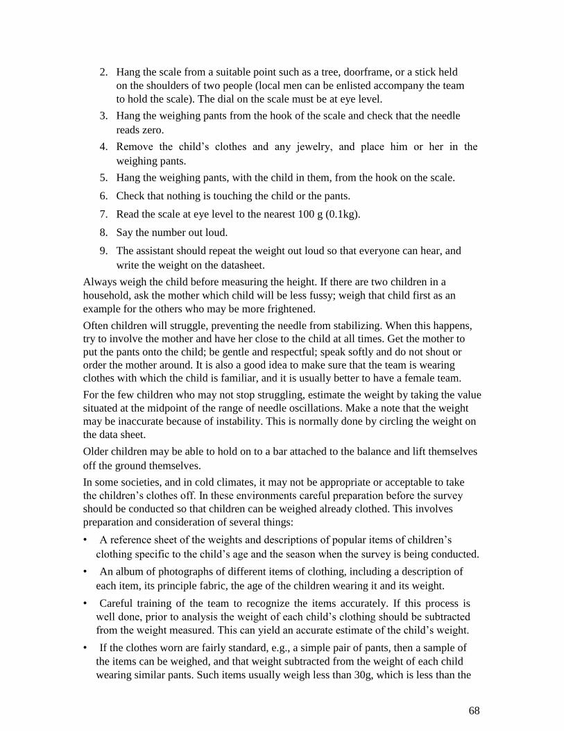
2. Hang the scale from a suitable point such as a tree, doorframe, or a stick held

on the shoulders of two people (local men can be enlisted accompany the team

to hold the scale). The dial on the scale must be at eye level.

3. Hang the weighing pants from the hook of the scale and check that the needle

reads zero.

4. Remove the child’s clothes and any jewelry, and place him or her in the

weighing pants.

5. Hang the weighing pants, with the child in them, from the hook on the scale.

6. Check that nothing is touching the child or the pants.

7. Read the scale at eye level to the nearest 100 g (0.1kg).

8. Say the number out loud.

9. The assistant should repeat the weight out loud so that everyone can hear, and

write the weight on the datasheet. Always weigh the child before measuring the height. If there are two children in a

household, ask the mother which child will be less fussy; weigh that child first as an

example for the others who may be more frightened. Often children will struggle, preventing the needle from stabilizing. When this happens,

try to involve the mother and have her close to the child at all times. Get the mother to

put the pants onto the child; be gentle and respectful; speak softly and do not shout or

order the mother around. It is also a good idea to make sure that the team is wearing

clothes with which the child is familiar, and it is usually better to have a female team. For the few children who may not stop struggling, estimate the weight by taking the value

situated at the midpoint of the range of needle oscillations. Make a note that the weight

may be inaccurate because of instability. This is normally done by circling the weight on

the data sheet. Older children may be able to hold on to a bar attached to the balance and lift themselves

off the ground themselves. In some societies, and in cold climates, it may not be appropriate or acceptable to take

the children’s clothes off. In these environments careful preparation before the survey

should be conducted so that children can be weighed already clothed. This involves

preparation and consideration of several things: • A reference sheet of the weights and descriptions of popular items of children’s

clothing specific to the child’s age and the season when the survey is being conducted. • An album of photographs of different items of clothing, including a description of

each item, its principle fabric, the age of the children wearing it and its weight. • Careful training of the team to recognize the items accurately. If this process is

well done, prior to analysis the weight of each child’s clothing should be subtracted

from the weight measured. This can yield an accurate estimate of the child’s weight. • If the clothes worn are fairly standard, e.g., a simple pair of pants, then a sample of

the items can be weighed, and that weight subtracted from the weight of each child

wearing similar pants. Such items usually weigh less than 30g, which is less than the 68

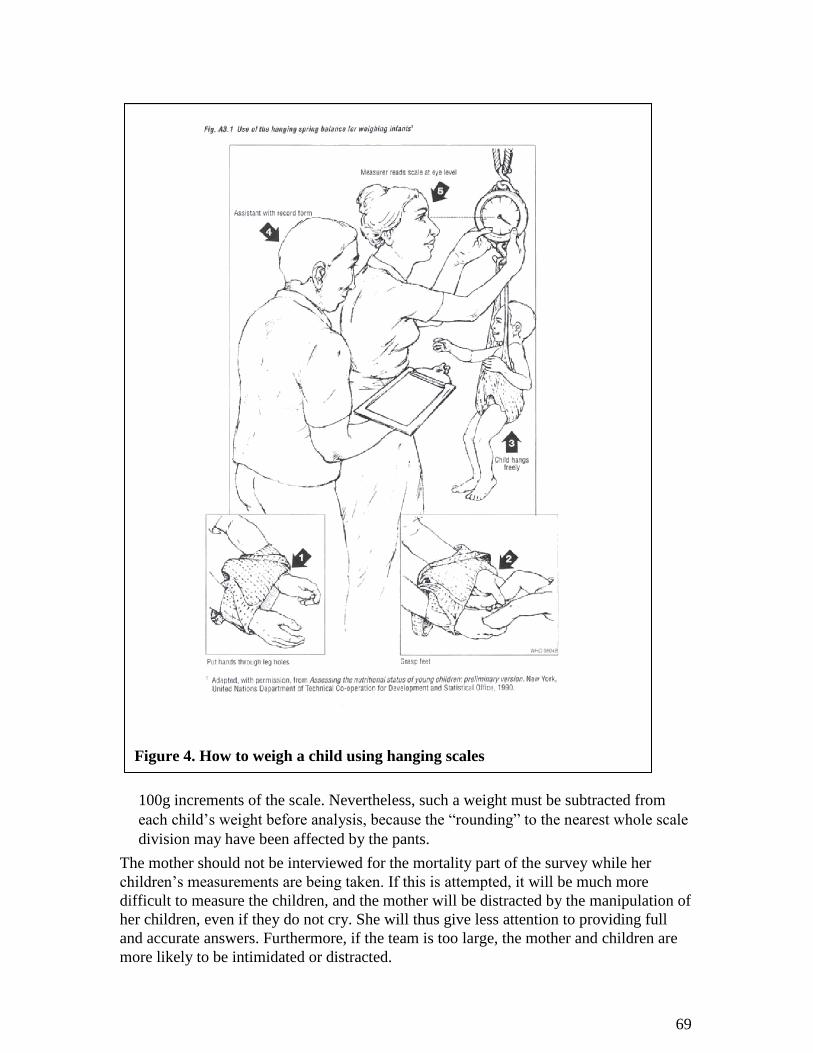
Figure 4. How to weigh a child using hanging scales

100g increments of the scale. Nevertheless, such a weight must be subtracted from

each child’s weight before analysis, because the “rounding” to the nearest whole scale

division may have been affected by the pants. The mother should not be interviewed for the mortality part of the survey while her

children’s measurements are being taken. If this is attempted, it will be much more

difficult to measure the children, and the mother will be distracted by the manipulation of

her children, even if they do not cry. She will thus give less attention to providing full

and accurate answers. Furthermore, if the team is too large, the mother and children are

more likely to be intimidated or distracted.

69

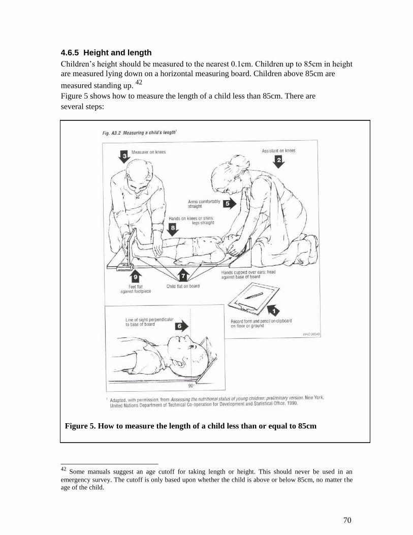
4.6.5 Height and length Children’s height should be measured to the nearest 0.1cm. Children up to 85cm in height

are measured lying down on a horizontal measuring board. Children above 85cm are

measured standing up. 42

Figure 5 shows how to measure the length of a child less than 85cm. There are

several steps:

Figure 5. How to measure the length of a child less than or equal to 85cm 42

Some manuals suggest an age cutoff for taking length or height. This should never be used in an

emergency survey. The cutoff is only based upon whether the child is above or below 85cm, no matter the age of the child.

70

1. Explain the procedure to the child’s mother or caregiver.

2. Remove the child’s shoes and any hair ornament or top knot on the top of the

child’s head.

3. Place the child gently onto the board on his/her back, with the head against the

fixed vertical part and the soles of the feet near the cursor or moving part. The

child should lie straight in the middle of the board, looking directly up.

4. The assistant should hold the child’s head firmly against the base of the board.

5. The measurer places one hand on the knees (to keep the legs straight), places the

child’s feet flat against the cursor with the other hand, and pushes the cursor

against the feet firmly but gently.

6. The measurer reads and announces the length to the nearest 0.1cm.

7. The assistant repeats the measurement out loud and records it on the datasheet. In some cultures, parents may be unhappy about measuring a child lying down, as such a

procedure is used to measure bodies for a coffin. In these populations, the measurement

technique is at best seen as bad luck, and it is particularly important to have local people

from the same culture as the main people on the team. It is also crucial that community

leaders, religious authorities, and other influential people understand why the

measurements are being made and give the teams explicit authority to make the length

measurements. The mother must understand this and give her permission specifically. In

these circumstances, children who can stand can have their height measured instead of

length, and a correction made to the measurement.

71

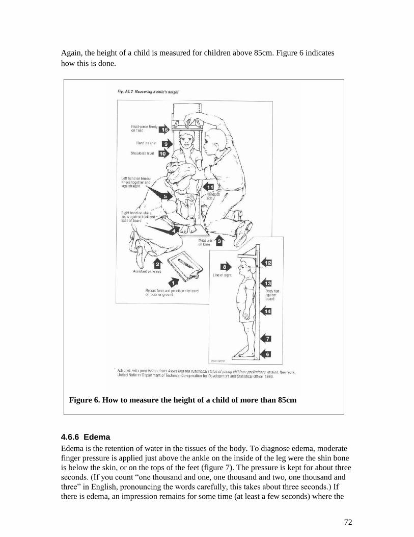
Again, the height of a child is measured for children above 85cm. Figure 6 indicates

how this is done.

Figure 6. How to measure the height of a child of more than 85cm 4.6.6 Edema Edema is the retention of water in the tissues of the body. To diagnose edema, moderate

finger pressure is applied just above the ankle on the inside of the leg were the shin bone

is below the skin, or on the tops of the feet (figure 7). The pressure is kept for about three

seconds. (If you count “one thousand and one, one thousand and two, one thousand and

three” in English, pronouncing the words carefully, this takes about three seconds.) If

there is edema, an impression remains for some time (at least a few seconds) where the 72

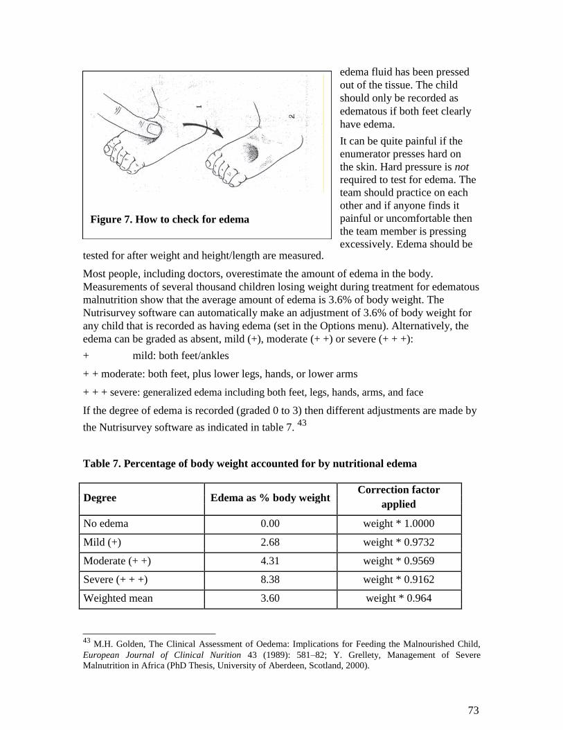
Figure 7. How to check for edema

tested for after weight and height/length are measured.

edema fluid has been pressed

out of the tissue. The child

should only be recorded as

edematous if both feet clearly

have edema. It can be quite painful if the

enumerator presses hard on

the skin. Hard pressure is not

required to test for edema. The

team should practice on each

other and if anyone finds it

painful or uncomfortable then

the team member is pressing

excessively. Edema should be

Most people, including doctors, overestimate the amount of edema in the body.

Measurements of several thousand children losing weight during treatment for edematous

malnutrition show that the average amount of edema is 3.6% of body weight. The

Nutrisurvey software can automatically make an adjustment of 3.6% of body weight for

any child that is recorded as having edema (set in the Options menu). Alternatively, the

edema can be graded as absent, mild (+), moderate (+ +) or severe (+ + +): + mild: both feet/ankles

+ + moderate: both feet, plus lower legs, hands, or lower arms

+ + + severe: generalized edema including both feet, legs, hands, arms, and face

If the degree of edema is recorded (graded 0 to 3) then different adjustments are made by

the Nutrisurvey software as indicated in table 7. 43

Table 7. Percentage of body weight accounted for by nutritional edema

Degree Edema as % body weight Correction factor

applied

No edema 0.00 weight * 1.0000

Mild (+) 2.68 weight * 0.9732

Moderate (+ +) 4.31 weight * 0.9569

Severe (+ + +) 8.38 weight * 0.9162

Weighted mean 3.60 weight * 0.964

43

M.H. Golden, The Clinical Assessment of Oedema: Implications for Feeding the Malnourished Child,

European Journal of Clinical Nurition 43 (1989): 581–82; Y. Grellety, Management of Severe

Malnutrition in Africa (PhD Thesis, University of Aberdeen, Scotland, 2000).

73

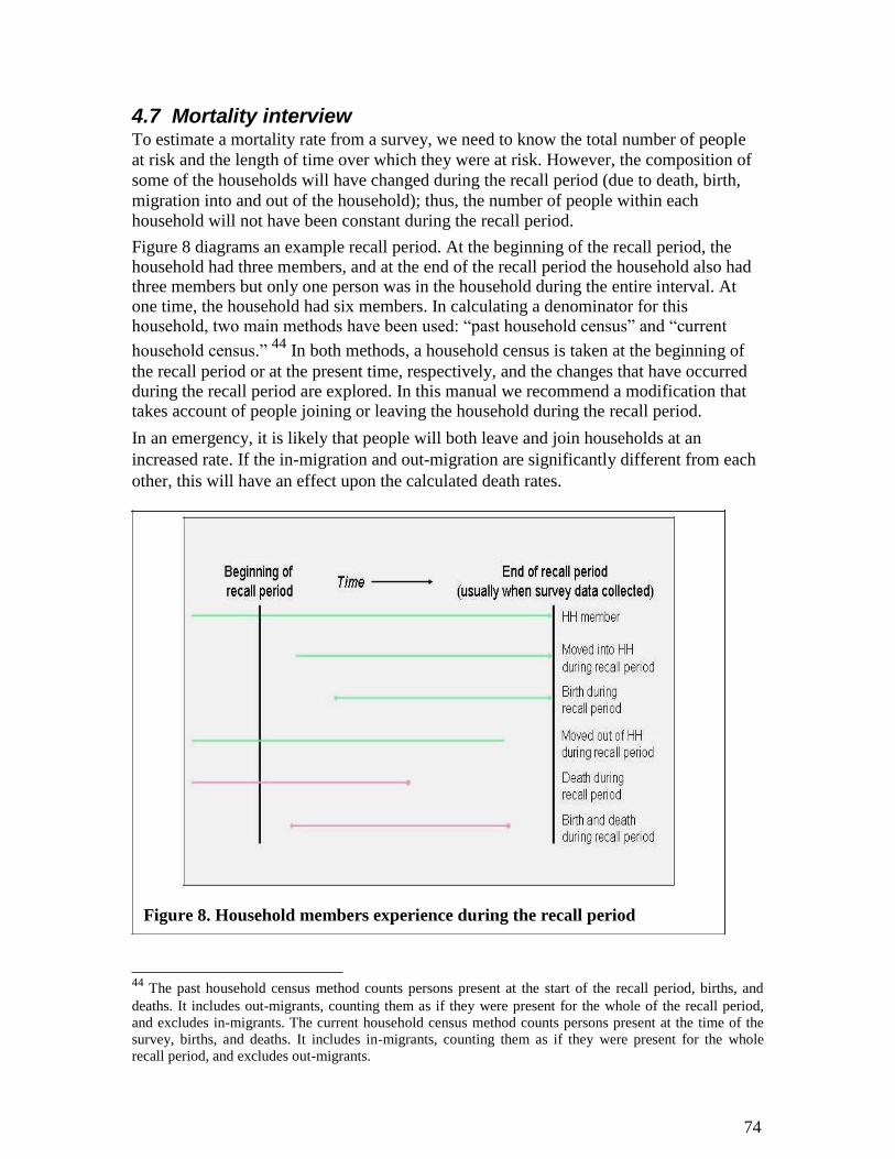
4.7 Mortality interview To estimate a mortality rate from a survey, we need to know the total number of people

at risk and the length of time over which they were at risk. However, the composition of

some of the households will have changed during the recall period (due to death, birth,

migration into and out of the household); thus, the number of people within each

household will not have been constant during the recall period. Figure 8 diagrams an example recall period. At the beginning of the recall period, the household had three members, and at the end of the recall period the household also had three members but only one person was in the household during the entire interval. At one time, the household had six members. In calculating a denominator for this household, two main methods have been used: “past household census” and “current

household census.” 44

In both methods, a household census is taken at the beginning of

the recall period or at the present time, respectively, and the changes that have occurred during the recall period are explored. In this manual we recommend a modification that takes account of people joining or leaving the household during the recall period. In an emergency, it is likely that people will both leave and join households at an

increased rate. If the in-migration and out-migration are significantly different from each

other, this will have an effect upon the calculated death rates.

Figure 8. Household members experience during the recall period

44

The past household census method counts persons present at the start of the recall period, births, and

deaths. It includes out-migrants, counting them as if they were present for the whole of the recall period,

and excludes in-migrants. The current household census method counts persons present at the time of the

survey, births, and deaths. It includes in-migrants, counting them as if they were present for the whole

recall period, and excludes out-migrants.

74

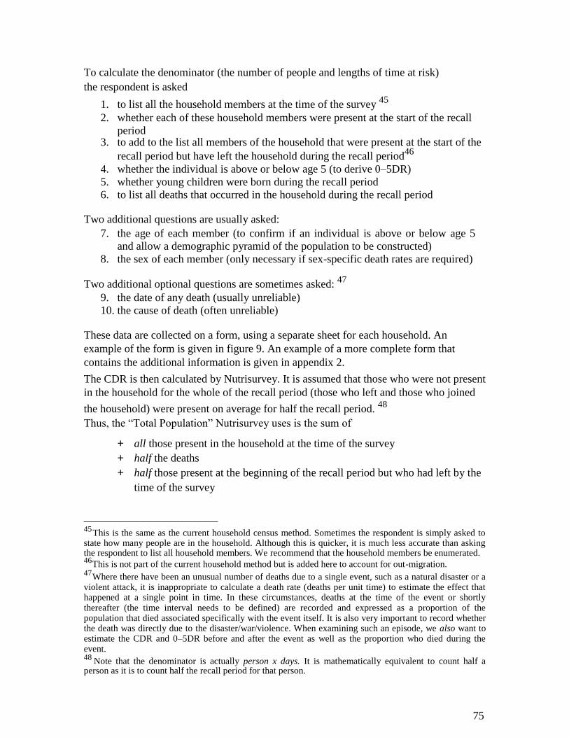
To calculate the denominator (the number of people and lengths of time at risk)

the respondent is asked

1. to list all the household members at the time of the survey 45

2. whether each of these household members were present at the start of the recall

period 3. to add to the list all members of the household that were present at the start of the

recall period but have left the household during the recall period46

4. whether the individual is above or below age 5 (to derive 0–5DR)

5. whether young children were born during the recall period

6. to list all deaths that occurred in the household during the recall period Two additional questions are usually asked:

7. the age of each member (to confirm if an individual is above or below age 5

and allow a demographic pyramid of the population to be constructed)

8. the sex of each member (only necessary if sex-specific death rates are required)

Two additional optional questions are sometimes asked: 47

9. the date of any death (usually unreliable)

10. the cause of death (often unreliable) These data are collected on a form, using a separate sheet for each household. An

example of the form is given in figure 9. An example of a more complete form that

contains the additional information is given in appendix 2. The CDR is then calculated by Nutrisurvey. It is assumed that those who were not present

in the household for the whole of the recall period (those who left and those who joined

the household) were present on average for half the recall period. 48

Thus, the “Total Population” Nutrisurvey uses is the sum of

+ all those present in the household at the time of the survey + half the deaths + half those present at the beginning of the recall period but who had left by the

time of the survey 45 This is the same as the current household census method. Sometimes the respondent is simply asked to state how many people are in the household. Although this is quicker, it is much less accurate than asking the respondent to list all household members. We recommend that the household members be enumerated.

46 This is not part of the current household method but is added here to account for out-migration.

47 Where there have been an unusual number of deaths due to a single event, such as a natural disaster or a violent attack, it is inappropriate to calculate a death rate (deaths per unit time) to estimate the effect that happened at a single point in time. In these circumstances, deaths at the time of the event or shortly thereafter (the time interval needs to be defined) are recorded and expressed as a proportion of the population that died associated specifically with the event itself. It is also very important to record whether the death was directly due to the disaster/war/violence. When examining such an episode, we also want to estimate the CDR and 0–5DR before and after the event as well as the proportion who died during the event.

48 Note that the denominator is actually person x days. It is mathematically equivalent to count half a person as it is to count half the recall period for that person.

75

Figure 9. Example of household enumeration data collection form

− half those present at the time of the survey but who joined the household

during the recall period.49

− subtract: half the births

49

If in- and out-migration are exactly balanced, counting half a person for each migrant is the same

mathematically as counting all in-migrants as whole persons and ignoring out-migrants in the current-

household method. It is also the same as counting out-migrants as whole people and ignoring in-migrants in

the past-household method. However, both in- and out-migration are frequently major coping strategies in a

disaster situation, and one is usually far greater than the other and will influence the final result. Therefore,

we suggest attempting to enumerate both in- and out-migration in an emergency survey. This is a bit like

combining the current and past household census methods together. Furthermore, in- and out-migration

rates can be easily calculated from the data and are useful to include in the survey report.

76

Infants that were born and died within the recall period are counted as deaths but are not

included in the denominator. The calculations are done automatically by Nutrisurvey.

4.7.1 Mass migration In an emergency situation whole families migrate. There are likely to be whole families

that arrive in the survey area during the recall period. Part of their experience will have

been in the study area, and part in the area from which they migrated. In the case of a

forming refugee/IDP camp, this can apply to a large proportion of the study population.

The mortality experience in the camp itself is likely to be very different from that

experienced before they departed from a stricken area or on the journey, which is usually

particularly hazardous. The various households will have arrived at different times.

Under these circumstances, if we take a fixed recall period, some of the respondent

households will have been in the camp for the whole period and some will be new

arrivals that have spent most of the recall period elsewhere or on the journey. In a camp situation, it is desirable to derive separate death rates for the time that the

population was in the camp and for the time before the displaced households reached the

camp. As the denominator for the death rate is person-days at risk, if we know how long

each household has been in the camp, we can calculate a death rate, but in this case the

recall period (or “period considered at risk”) is different for each household. The date of

arrival can often be determined from a registration card given to new arrivals. Arrival is

also an important date that most migrating households remember. In this case, the date of

arrival is recorded for each household, and the time period used in the equation is the

average number of days each household has spent in the camp. To derive the separate mortality rate for the time before arrival, the fixed recall period is

used, as in the standard method, and the average time spent in the camp subtracted from

this time. Deaths are recorded as occurring in the camp or before arrival but after the

start of the recall period. The “before arrival” mortality rate is much more susceptible to

serious sampling error, because the households are self-selected in terms of those that

have the means, opportunity, and composition that enable them to migrate, and the

households may have arrived from a wide variety of different geographical areas. The

rate thus only applies to the migrants who have reached the camp and should not be

extrapolated to the area of origin. It is much more difficult to calculate the sample size needed to separate CDR into two

components—before and after arrival. There is an added variable in the calculation: the

average length of time households have spent in the camp. In effect it is like doing two

surveys using the same households: one for the time in the camp and one for the time

before arrival. If the average length of time in the camp can be obtained from the

camp’s administrators, this is used as one of the “recall periods” in the calculation.

4.7.2 Determining cause of death Inquiry into cause of death should be limited to causes that are clearly defined by local

terms and familiar to the local population. These include measles, neonatal tetanus, and

diarrhea. If local terms do not exist, inquiry should be limited to deaths due to violence

77

and all other causes. Violent deaths can be due to war injuries and atrocities, or accidents

not related directly to conflict. In this case two questions are sufficient:

1.“Did [the person] die from some sort of violence such as being assaulted, shot or

violated, a car accident, fall, drowning, poisoning, burn, bite or sting?” If YES, Go to next question.

If NO, record death not related to injury or violence.

2.“Was this injury caused by someone fighting the war such as from a bullet, bomb,

mine, machete or assault?” If NO, record non-war-related injury or violence as cause of death.

If YES, record war-related injury or violence as cause of death. As with other parts of the household questionnaire, questions about cause of death need

to be translated into the local language, back-translated to the original language to ensure

accurate translation, and pretested in the local setting. Usually the head of household is

interviewed; however, there may be a need to interview multiple respondents if the

current head is a child or a relative who has lived only part of the recall period in the

household.

4.8 Analysis of results The report should always be presented in a standard format and contain all the

information that allows the reader to understand why the survey was conducted, the

methods used, the population to which the results apply, the results themselves, any

additional relevant information, and a summary of problems encountered. The report can

also contain recommendations. These recommendations should not be simply general

recommendations, but should be directly supported and justified by the data in the report.

The presentation of the information in a standard way ensures that no important

information is omitted. It also allows a reader who is familiar with the format to quickly

find the particular information he or she is looking for. The Nutrisurvey software takes

the data that have been entered during the survey, does the analysis, and presents the data

in a standard format. It also gives headings of all the paragraphs that need to be

completed by the person responsible for the report.

78

5 Using Nutrisurvey software, step-by-step A SMART survey is designed to be analyzed by computer using the Nutrisurvey

software. It can be downloaded free from either www.smartindicators.org or from

www.nutrisurvey.de/ena/ena.html. The food security component is analyzed using a

separate Excel spreadsheet that is not yet included in the software. The analysis can also be done using other programs or by hand, although this is not

recommended for non-epidemiologists. The first screen of the Nutrisurvey software program is the anthropometry data

entry screen.

The various sheets on the front-end are used in order. 50

The steps for using

Nutrisurvey are as follows:

1. Planning the survey.

2. Training the teams.

3. Entering the nutritional (anthropometric and edema) data.

4. Entering the mortality data.

5. Checking the data for errors and plausibility. 51

a. Highlighting implausible values.

b. Analysis for digit preference.

c. Analysis by team.

d. Comparison of the prevalence of severe malnutrition calculated from

the mean and standard deviation with the prevalence from counting

the subjects below the cut-off points.

6. Generating the results.

7. Writing the report using a standard format.

5.1 Planning the survey Figure 10 shows the Nutrisurvey survey planning screen. The survey must be given

a unique name (see the section on “Naming of files” below). The software cannot help decide what type of sampling will be conducted.

1. The survey will either be a random sample (simple random or systematic random)

or a cluster survey. Check the appropriate box. 50 As the software is under continuous development, the version downloaded may not be exactly the same as that shown here. The “update” notes that are downloaded with the software should be consulted for a full description of the current version.

51 In future versions, the distribution of the data will also be examined.

79

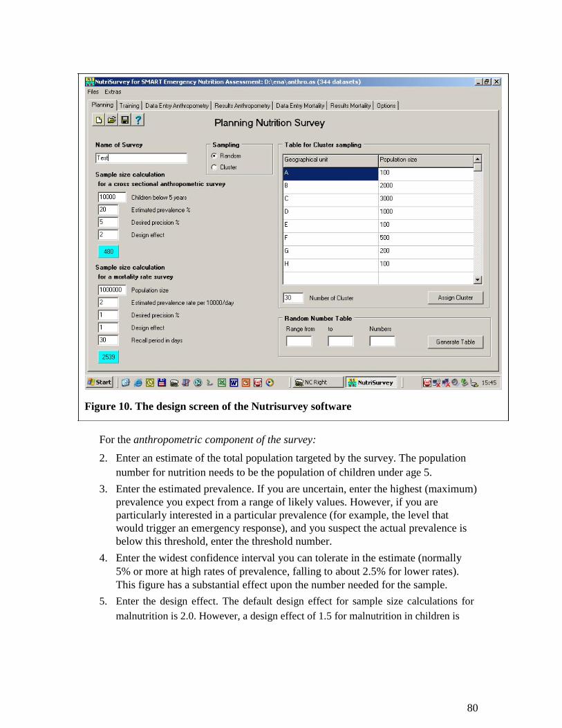
Figure 10. The design screen of the Nutrisurvey software

For the anthropometric component of the survey: 2. Enter an estimate of the total population targeted by the survey. The population

number for nutrition needs to be the population of children under age 5. 3. Enter the estimated prevalence. If you are uncertain, enter the highest (maximum)

prevalence you expect from a range of likely values. However, if you are

particularly interested in a particular prevalence (for example, the level that

would trigger an emergency response), and you suspect the actual prevalence is

below this threshold, enter the threshold number. 4. Enter the widest confidence interval you can tolerate in the estimate (normally

5% or more at high rates of prevalence, falling to about 2.5% for lower rates).

This figure has a substantial effect upon the number needed for the sample. 5. Enter the design effect. The default design effect for sample size calculations for

malnutrition is 2.0. However, a design effect of 1.5 for malnutrition in children is

80

often sufficient. The decision should be made individually for each emergency

context. 52

The results of steps 1–5 yield the total number of children required for the sample

(sample size). This figure will be automatically calculated and will appear in the blue

box. In cluster surveys, this number should be divided by the number of households

that can be visited each day. This will provide the number of clusters. For the mortality component of the survey:

1. Enter an estimate of the total population targeted by the survey. The

population number for mortality needs to be the total population.

2. Enter the expected mortality rate (/10,000 persons/day).

3. Enter the required precision (/10,000 persons/day). For example, if your

expected mortality rate is 2.0/10,000 persons/day and you want a confidence

interval of 1.4–2.6, enter a required precision of 0.6 (i.e., 2.0 ± 0.6 = 1.4–2.6).

The precision chosen has a substantial effect upon the sample size needed.

4. Enter the design effect. The default design effect for sample size calculations

for mortality is 2.0. If violence-related-mortality is limited, a design effect of

1.5 for crude death rate may also be sufficient.

5. Enter the chosen recall period in days. In most situations, a recall period of

approximately 90 days (or between 30 to 120) days will be used. However,

the decision should be made individually for each emergency context. This

will depend upon the time of a “memorable event,” and this is rarely exactly

90 days. The recall period also has a substantial effect upon the number of

households that will need to be interviewed.

6. Divide the sample number by the average household size. This will give

the number of households that should be visited to achieve the sample size.

5.1.1 Choosing the clusters

5.1.1.1 Enter the number of clusters

There should always be at least 30 clusters. Twenty-six clusters is the minimum for the

survey to be valid. The best way to obtain the number of clusters is to decide realistically

the number of households that can be visited in one day. The higher of the two values,

(a) the total sample size of children (assuming an average of one eligible child per

household visited), or (b) the total households needed for the mortality survey, is divided

by the number of households that can be visited in one day. This is the number of

clusters that should be chosen if it is equal to or more than 30. Otherwise, 30 clusters

should be used. If there is a choice, it is better to increase the number of clusters and

reduce the numbers of children in each cluster.

52

Research is presently underway to examine the distribution of design effects in well-conducted surveys.

The range of design effects that are often found under different circumstances will be included in later

versions of the SMART methodology.

81

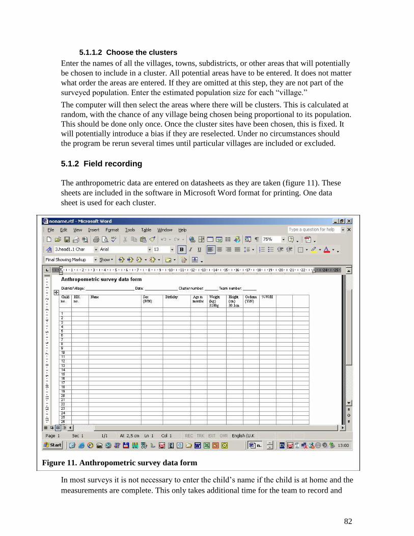
5.1.1.2 Choose the clusters Enter the names of all the villages, towns, subdistricts, or other areas that will potentially

be chosen to include in a cluster. All potential areas have to be entered. It does not matter

what order the areas are entered. If they are omitted at this step, they are not part of the

surveyed population. Enter the estimated population size for each “village.”

The computer will then select the areas where there will be clusters. This is calculated at

random, with the chance of any village being chosen being proportional to its population.

This should be done only once. Once the cluster sites have been chosen, this is fixed. It

will potentially introduce a bias if they are reselected. Under no circumstances should

the program be rerun several times until particular villages are included or excluded.

5.1.2 Field recording

The anthropometric data are entered on datasheets as they are taken (figure 11). These

sheets are included in the software in Microsoft Word format for printing. One data

sheet is used for each cluster.

Figure 11. Anthropometric survey data form

In most surveys it is not necessary to enter the child’s name if the child is at home and the

measurements are complete. This only takes additional time for the team to record and 82

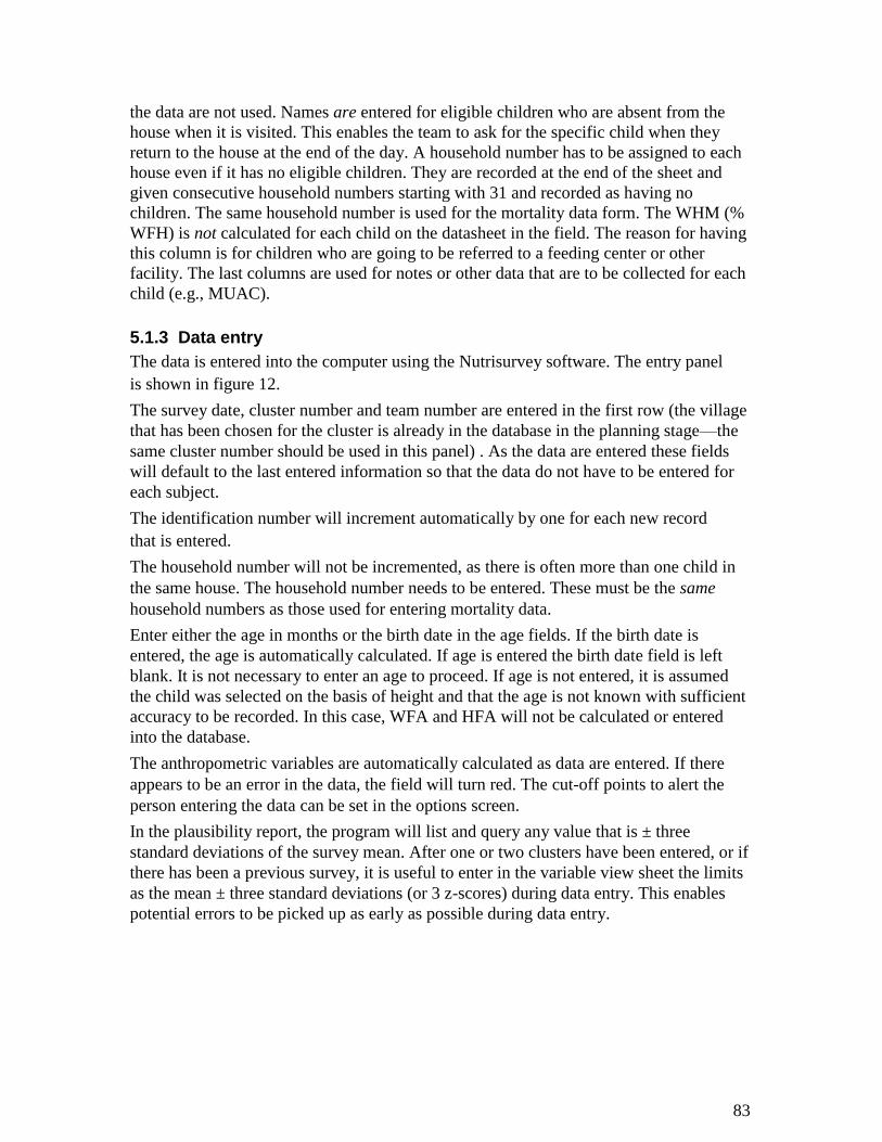
the data are not used. Names are entered for eligible children who are absent from the

house when it is visited. This enables the team to ask for the specific child when they

return to the house at the end of the day. A household number has to be assigned to each

house even if it has no eligible children. They are recorded at the end of the sheet and

given consecutive household numbers starting with 31 and recorded as having no

children. The same household number is used for the mortality data form. The WHM (%

WFH) is not calculated for each child on the datasheet in the field. The reason for having

this column is for children who are going to be referred to a feeding center or other

facility. The last columns are used for notes or other data that are to be collected for each

child (e.g., MUAC).

5.1.3 Data entry The data is entered into the computer using the Nutrisurvey software. The entry panel

is shown in figure 12. The survey date, cluster number and team number are entered in the first row (the village

that has been chosen for the cluster is already in the database in the planning stage—the

same cluster number should be used in this panel) . As the data are entered these fields

will default to the last entered information so that the data do not have to be entered for

each subject. The identification number will increment automatically by one for each new record

that is entered. The household number will not be incremented, as there is often more than one child in

the same house. The household number needs to be entered. These must be the same

household numbers as those used for entering mortality data. Enter either the age in months or the birth date in the age fields. If the birth date is

entered, the age is automatically calculated. If age is entered the birth date field is left

blank. It is not necessary to enter an age to proceed. If age is not entered, it is assumed

the child was selected on the basis of height and that the age is not known with sufficient

accuracy to be recorded. In this case, WFA and HFA will not be calculated or entered

into the database. The anthropometric variables are automatically calculated as data are entered. If there

appears to be an error in the data, the field will turn red. The cut-off points to alert the

person entering the data can be set in the options screen. In the plausibility report, the program will list and query any value that is ± three

standard deviations of the survey mean. After one or two clusters have been entered, or if

there has been a previous survey, it is useful to enter in the variable view sheet the limits

as the mean ± three standard deviations (or 3 z-scores) during data entry. This enables

potential errors to be picked up as early as possible during data entry. 83

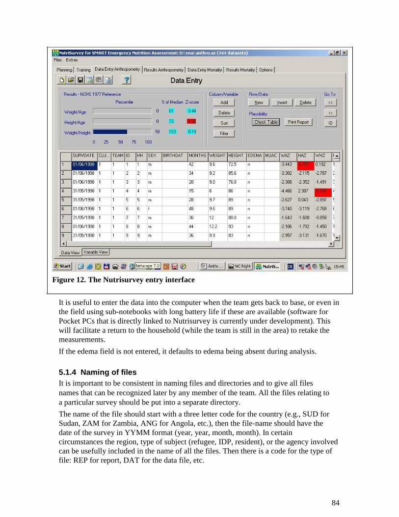
Figure 12. The Nutrisurvey entry interface

It is useful to enter the data into the computer when the team gets back to base, or even in

the field using sub-notebooks with long battery life if these are available (software for

Pocket PCs that is directly linked to Nutrisurvey is currently under development). This

will facilitate a return to the household (while the team is still in the area) to retake the

measurements.

If the edema field is not entered, it defaults to edema being absent during analysis.

5.1.4 Naming of files It is important to be consistent in naming files and directories and to give all files

names that can be recognized later by any member of the team. All the files relating to

a particular survey should be put into a separate directory.

The name of the file should start with a three letter code for the country (e.g., SUD for

Sudan, ZAM for Zambia, ANG for Angola, etc.), then the file-name should have the

date of the survey in YYMM format (year, year, month, month). In certain

circumstances the region, type of subject (refugee, IDP, resident), or the agency involved

can be usefully included in the name of all the files. Then there is a code for the type of

file: REP for report, DAT for the data file, etc.

84

This naming convention means that if the files in the directory are sorted they will

automatically be listed in a clear order and all the files pertaining to a particular survey

will be together. All files related to one survey should be kept in a unique directory. The

directory should also be named using the same convention (by country and date), and

any other information that makes the directory unique for a particular survey. It is

important that everyone in an agency uses the standard convention for naming files. Thus, a file named <LIB_0408_rep.doc> would be the report of a survey taken in August

2004 in Liberia. There may be several simultaneous surveys conducted in Liberia around

that time, <LIB_0409_IDP_Buchanan_AAH_dat.xls> would be the data file for a survey

with IDPs in Buchanan, Liberia in September 2004 conducted by Action Against

Hunger. Under no circumstances should the files be called “report.doc” or

“SupervisorsName.doc.”

5.1.5 Data preparation and cleaning Before doing the definitive analysis, any errors in the data need to be identified and, if

possible, corrected. This is done partly during data entry. An implausible or “out-of-

range” value is colored red during data entry. The ranges should be set in the variable

view sheet before data entry. Data cleaning is also done using Nutrisurvey’s “plausibility” check. The computer

automatically examines the data to see if there are values outside the usual or expected

range and lists them in Microsoft Word. These values should be reviewed and checked

against the original written data collection sheets. Any error in data entry should be

corrected immediately.

5.1.5.1 Missing data

If certain critical pieces of information are missing from a child’s survey record, it will

not be possible to include the child in some of the anthropometric data analyses: Age: If information on age is missing, you can still include the child in the assessment of

wasting and edema, because these do not require age. However, you will need to be sure

the child is eligible to be in the survey (i.e., in the required height range of 65cm–110cm). Sex: If information on sex is missing you should still include the child in the assessment

of wasting and edema. The reference population information on height and weight is

sex specific. However, the difference between the sexes in terms of the WFH reference

standards is small, and irrelevant for edema. Height: If information on height is missing you cannot include the child in the

assessment of wasting. However, the child can still be included in an analysis of

edema, because any child with edema is severely malnourished. Weight: If information on weight is missing you cannot include the child in the assessment

of wasting. However, the child can still be included in an analysis of edema.

5.1.5.2 Data outside the required range

In most nutrition surveys, we are measuring children aged 6–59 months, or children who

are 65cm–110cm tall. Children outside these ranges should not be included in the results.

These values depend upon the defaults that have been set in the variable view sheet of the

85

software. The default is to accept any child who is in the correct age range, even if the

height is out of range. Any child outside the age range will be marked by the program.

If height data are missing, the anthropometric indices of interest cannot be calculated.

However, if the age is within range, the child can be included if there is edema. The

accepted height range can be altered in the variable view sheet, for example, to change

the range to 60cm–100cm if the population is very stunted. These choices must be

included in the report. Thus, by default, if a child is 55 months old and 112cm the child will be included.

However, if the child is 65 months old, it should not be included and the computer

will automatically exclude the child in the results.

5.1.5.3 Extreme WFH data

In addition to excluding children with missing information, or who are out of the required

range, we also want to exclude children who have a WFH that is more likely to be the

result of an error than a true measurement. There are various ways of doing this. Clearly,

data that are biologically unlikely are very likely to be the result of a measurement or

recording error. Thus, it is very unusual in an emergency context to find any child with a

WHZ < –5.00 or a WHZ > +3.00. Most children with wrongly measured data give values that are within the plausible

range. Inclusion of such errors can be surmised from examination of the standard

deviation, and other statistical checks on the data. The standard deviation should be

between 0.8 and 1.2 z-score units for WFH in all well-conducted surveys (in 80% of

surveys the standard deviation is between 0.9 and 1.1 z-score units). The standard

deviation increases as the proportion of erroneous results in the dataset increases; this

has a very dramatic effect upon the computed prevalence of wasting. For this reason, if a

value is more likely to be an error than a real measurement, it should be removed from

the analysis. We do this by taking the mean of the WFH data as the fixed point for

describing the status of the population we are surveying. Statistically about 2.5 children

out of 900 will lie outside the limits of ±3 z-score units of the mean. Less than 0.5 out of

1,000 will lie outside ±3.5 z-score units from the mean. This forms the basis for deciding

if a value is more likely to be an error than a real measurement. The software will list

children with these extreme values in the plausibility check list.

5.1.5.4 Checking for measurement bias

Measurement bias occurs when the team has not been adequately trained or supervised or

when the measuring equipment is faulty. The best way to avoid measurement bias is to

be rigorous in training and supervision and put in place careful checks to assure the

quality of the equipment. Supervisors should check data collection forms at the end of

each day to see if WHZ are feasible and within the plausibility range, and to see if edema

is being realistically reported. There are several useful methods to check the quality of the anthropometric data

collected during a nutrition assessment after the data has been collected: First, the distribution of the final decimal for height and weight. This will tell you if the

team members are rounding weights and height to the nearest kilogram or centimeter,

respectively. This phenomenon is called “digit preference.” Nutrisurvey automatically 86

examines the data for digit preference. Furthermore, it examines the digit preference for

each of the teams. There may be one team that is “cutting corners” or has been

improperly trained or supervised. The data can then be examined to see if there is a

substantial difference if the data from that team is omitted. Second, the standard deviation of the z-scores for WFH and HFA should be examined.

As explained in the section on extreme values, this tells you if there is substantial random

error in the measurements. If the standard deviation is high (over 1.2), it is likely that

there are a lot of extreme values and values more than ±3 z-scores of the mean.

Nutrisurvey not only examines the standard deviation for the whole survey, but it also

calculates the standard deviation for each team’s measurements and the number of

extreme values for each team. The standard deviation and prevalence of malnutrition can

then be examined omitting the data from one team. Comparison of the data with and

without that particular team’s results should be undertaken to see if there is a substantial

difference. Any problems should be reported. There are other statistical measures that are computed on the data and for each team’s

results. First is skewness, which measures the extent to which the results are

symmetrical. The “moment of skewness” should lie between 1 and –1. Similarly, kurtosis

measures whether the tails are very long (Mexican hat) or very short (pudding shaped),

with too many values in the shoulders of the distribution. The “moment of kurtosis”

should also lie between 1 and –1. These variables can also be computed for each team,

and with one team omitted. It is extremely difficult to fabricate data for weight and

height that “pass” all these checks for data distribution. In particular, the kurtosis checks

whether values that might be considered to be an error by the team have been removed

(sometimes referred to as “overcleaning”). If any of the distribution checks are abnormal,

the survey may be biased and the results unreliable. There is a further check that can be made with a cluster survey. If the number of

individuals with wasting in each cluster is calculated, there will be one number for each

cluster. These numbers should follow a statistical distribution called a Poisson

distribution. The program tests whether the numbers follow this distribution

statistically. If the distribution is not Poisson, it means the population forming the

sample is heterogeneous, with “pockets of malnutrition” and areas that are spared.

These problems are often caused by the design of the survey, nonrandom selection of

the villages to contain the clusters, biased selection of houses in some areas, or

excessive heterogeneity in the surveyed population. The Nutrisurvey software

automatically calculates the Poisson distribution for wasting and compares this with the

expected distribution. If the data do not follow a Poisson distribution, there will also be

a larger than usual design effect. These two statistics give complementary information. When we examine many surveys, we find that the clusters with edema do not follow a

Poisson distribution, as they should if the whole population were equally vulnerable. In

fact, edema follows what is called a “negative binomial” distribution, which means that

there are some villages where lots of children get edema and others that are relatively

protected. This design effect for edema is usually larger than for wasting, and this

complicates calculation of the confidence intervals for severe malnutrition. If there is no substantial digit preference, the standard deviation is between 0.8 and 1.2,

the moments of skewness and kurtosis are within the range of 1 to –1, and the distribution

of wasting follows a Poisson distribution, then one can be reasonably confident that the

87

survey has been properly conducted, the sampling method is a fair representation of the

population, and the results can be relied upon. Even if there is no immediate intervention expected to address stunting, calculating the

HFA z-scores and their standard distribution should also be examined. The most usual

reason for a problem with the HFA data is determination of age. Once the data have been cleaned and examined to ensure they are plausible, we

proceed to the final analysis.

5.1.6 Analysis and reporting The graphs of the distribution of the combined variables, by gender, should be examined.

The data are automatically analyzed and reported as a Microsoft Word file. The headings

are generated. The survey supervisor should go through each heading and enter the

relevant information. The quantitative data are presented in the tables. To put the illustrations into the report, the graphs are transferred to the clipboard

within Nutrisurvey and pasted into the report at the appropriate place.

88

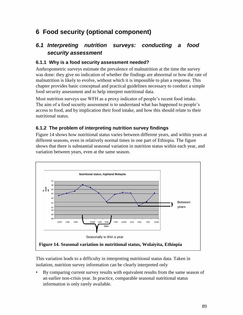
6 Food security (optional component)

6.1 Interpreting nutrition surveys: conducting a food

security assessment 6.1.1 Why is a food security assessment needed? Anthropometric surveys estimate the prevalence of malnutrition at the time the survey

was done: they give no indication of whether the findings are abnormal or how the rate of

malnutrition is likely to evolve, without which it is impossible to plan a response. This

chapter provides basic conceptual and practical guidelines necessary to conduct a simple

food security assessment and to help interpret nutritional data. Most nutrition surveys use WFH as a proxy indicator of people’s recent food intake.

The aim of a food security assessment is to understand what has happened to people’s

access to food, and by implication their food intake, and how this should relate to their

nutritional status.

6.1.2 The problem of interpreting nutrition survey findings Figure 14 shows how nutritional status varies between different years, and within years at

different seasons, even in relatively normal times in one part of Ethiopia. The figure

shows that there is substantial seasonal variation in nutrition status within each year, and

variation between years, even at the same season.

Nutritional status, highland Wolayita

97

96

%

med

ian

95

94

93

W / H

92 Between

M e a n

91 years

90

89

88

10/97 1/98 4/98 10/98 1/99 4/99 7/99 10/99 1/00 4/00 7/00 10/00

Date

Seasonally w ithin a year

Figure 14. Seasonal variation in nutritional status, Wolaiyita, Ethiopia

This variation leads to a difficulty in interpreting nutritional status data. Taken in

isolation, nutrition survey information can be clearly interpreted only • By comparing current survey results with equivalent results from the same season of

an earlier non-crisis year. In practice, comparable seasonal nutritional status

information is only rarely available. 89

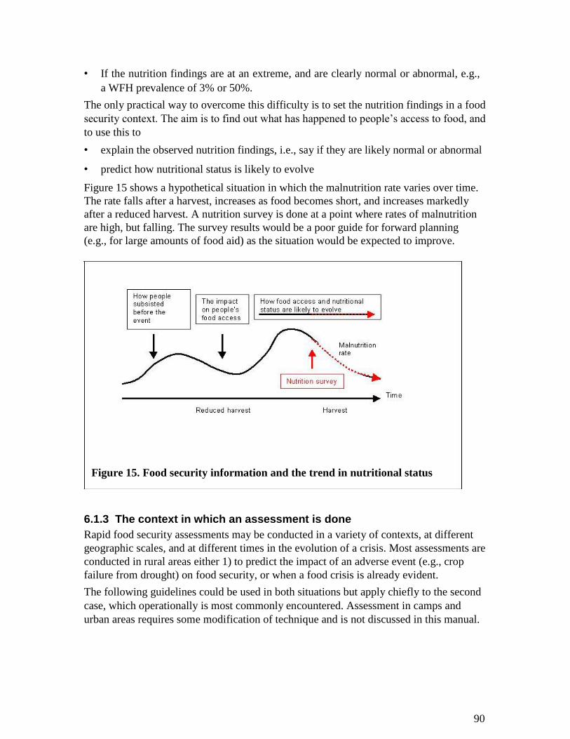
• If the nutrition findings are at an extreme, and are clearly normal or abnormal, e.g.,

a WFH prevalence of 3% or 50%. The only practical way to overcome this difficulty is to set the nutrition findings in a food

security context. The aim is to find out what has happened to people’s access to food, and

to use this to • explain the observed nutrition findings, i.e., say if they are likely normal or abnormal • predict how nutritional status is likely to evolve Figure 15 shows a hypothetical situation in which the malnutrition rate varies over time.

The rate falls after a harvest, increases as food becomes short, and increases markedly

after a reduced harvest. A nutrition survey is done at a point where rates of malnutrition

are high, but falling. The survey results would be a poor guide for forward planning

(e.g., for large amounts of food aid) as the situation would be expected to improve.

Figure 15. Food security information and the trend in nutritional status

6.1.3 The context in which an assessment is done Rapid food security assessments may be conducted in a variety of contexts, at different

geographic scales, and at different times in the evolution of a crisis. Most assessments are

conducted in rural areas either 1) to predict the impact of an adverse event (e.g., crop

failure from drought) on food security, or when a food crisis is already evident. The following guidelines could be used in both situations but apply chiefly to the second

case, which operationally is most commonly encountered. Assessment in camps and

urban areas requires some modification of technique and is not discussed in this manual. 90

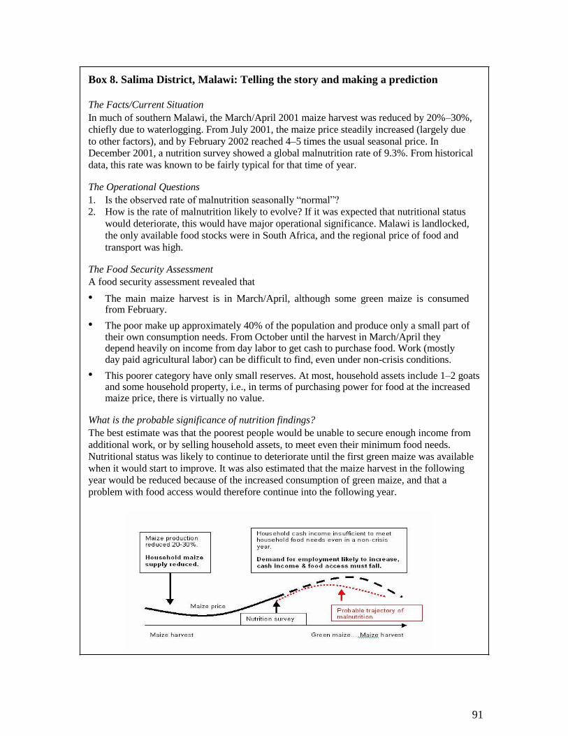
Box 8. Salima District, Malawi: Telling the story and making a prediction

The Facts/Current Situation In much of southern Malawi, the March/April 2001 maize harvest was reduced by 20%–30%,

chiefly due to waterlogging. From July 2001, the maize price steadily increased (largely due

to other factors), and by February 2002 reached 4–5 times the usual seasonal price. In

December 2001, a nutrition survey showed a global malnutrition rate of 9.3%. From historical

data, this rate was known to be fairly typical for that time of year. The Operational Questions 1. Is the observed rate of malnutrition seasonally “normal”?

2. How is the rate of malnutrition likely to evolve? If it was expected that nutritional status

would deteriorate, this would have major operational significance. Malawi is landlocked,

the only available food stocks were in South Africa, and the regional price of food and

transport was high. The Food Security Assessment A food security assessment revealed that • The main maize harvest is in March/April, although some green maize is consumed

from February. • The poor make up approximately 40% of the population and produce only a small part of

their own consumption needs. From October until the harvest in March/April they depend heavily on income from day labor to get cash to purchase food. Work (mostly day paid agricultural labor) can be difficult to find, even under non-crisis conditions.

• This poorer category have only small reserves. At most, household assets include 1–2 goats and some household property, i.e., in terms of purchasing power for food at the increased maize price, there is virtually no value.

What is the probable significance of nutrition findings? The best estimate was that the poorest people would be unable to secure enough income from

additional work, or by selling household assets, to meet even their minimum food needs.

Nutritional status was likely to continue to deteriorate until the first green maize was available

when it would start to improve. It was also estimated that the maize harvest in the following

year would be reduced because of the increased consumption of green maize, and that a

problem with food access would therefore continue into the following year.

91

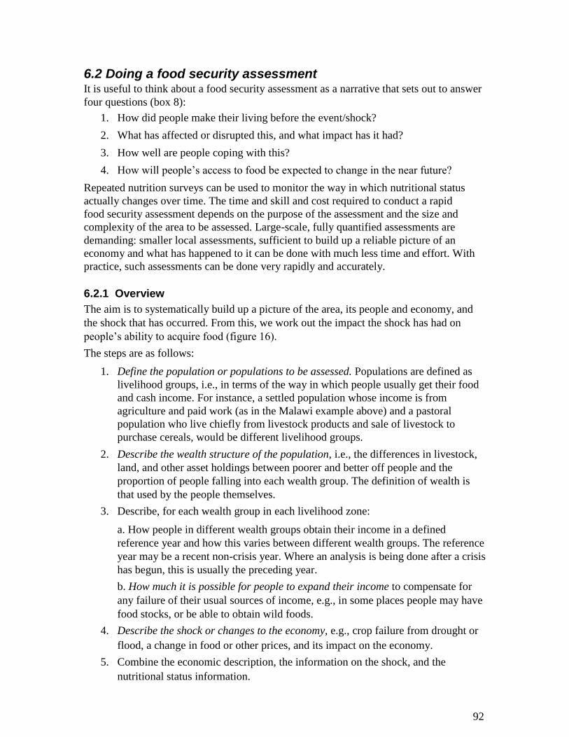
6.2 Doing a food security assessment It is useful to think about a food security assessment as a narrative that sets out to answer

four questions (box 8):

1. How did people make their living before the event/shock?

2. What has affected or disrupted this, and what impact has it had?

3. How well are people coping with this?

4. How will people’s access to food be expected to change in the near future? Repeated nutrition surveys can be used to monitor the way in which nutritional status

actually changes over time. The time and skill and cost required to conduct a rapid

food security assessment depends on the purpose of the assessment and the size and

complexity of the area to be assessed. Large-scale, fully quantified assessments are

demanding: smaller local assessments, sufficient to build up a reliable picture of an

economy and what has happened to it can be done with much less time and effort. With

practice, such assessments can be done very rapidly and accurately.

6.2.1 Overview The aim is to systematically build up a picture of the area, its people and economy, and

the shock that has occurred. From this, we work out the impact the shock has had on

people’s ability to acquire food (figure 16). The steps are as follows:

1. Define the population or populations to be assessed. Populations are defined as

livelihood groups, i.e., in terms of the way in which people usually get their food

and cash income. For instance, a settled population whose income is from

agriculture and paid work (as in the Malawi example above) and a pastoral

population who live chiefly from livestock products and sale of livestock to

purchase cereals, would be different livelihood groups.

2. Describe the wealth structure of the population, i.e., the differences in livestock,

land, and other asset holdings between poorer and better off people and the

proportion of people falling into each wealth group. The definition of wealth is

that used by the people themselves.

3. Describe, for each wealth group in each livelihood zone:

a. How people in different wealth groups obtain their income in a defined

reference year and how this varies between different wealth groups. The reference

year may be a recent non-crisis year. Where an analysis is being done after a crisis

has begun, this is usually the preceding year.

b. How much it is possible for people to expand their income to compensate for

any failure of their usual sources of income, e.g., in some places people may have

food stocks, or be able to obtain wild foods.

4. Describe the shock or changes to the economy, e.g., crop failure from drought or

flood, a change in food or other prices, and its impact on the economy.

5. Combine the economic description, the information on the shock, and the

nutritional status information.

92

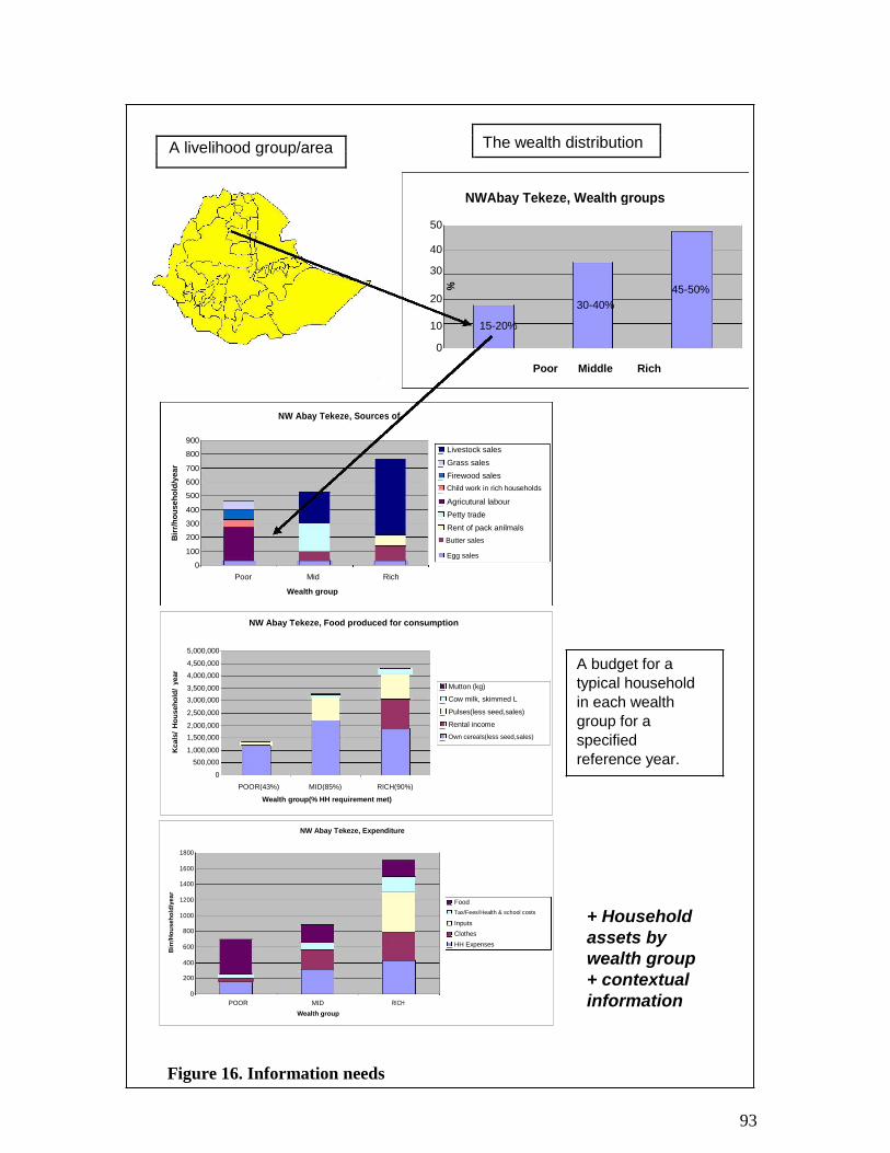
The wealth distribution

A livelihood group/area

NWAbay Tekeze, Wealth groups

50

40

30

%

45-50%

20

30-40%

10 15-20%

0

Poor Middle Rich

NW Abay Tekeze, Sources of

900

800

Bir

r/h

ou

se

ho

ld/y

ea

r 700

600

500

400

300

200

100

0

Poor Mid Rich

Wealth group

Livestock sales Grass sales Firewood sales Child work in rich households Agricutural labour Petty trade Rent of pack anilmals Butter sales

Egg sales

NW Abay Tekeze, Food produced for consumption

5,000,000

4,500,000

year

4,000,000

3,500,000

Ho

useh

old

/

3,000,000

2,500,000

2,000,000

Kcals

/

1,500,000

1,000,000

500,000

0

POOR(43%) MID(85%) RICH(90%)

Wealth group(% HH requirement met)

Mutton (kg) Cow milk, skimmed L Pulses(less seed,sales) Rental income Own cereals(less seed,sales)

A budget for a

typical household

in each wealth

group for a

specified

reference year.

NW Abay Tekeze, Expenditure

1800

1600

1400

Bir

r/H

ou

se

ho

ld/y

ea

r

1200

1000

800

600

400

200

0

POOR MID RICH

Wealth group

Food Tax/Fees/Health & school costs Inputs Clothes HH Expenses

+ Household

assets by

wealth group

+ contextual

information

Figure 16. Information needs

93

6.2.2 Getting the information On a rapid assessment, there is usually little

time for background research or detailed

quantitative surveys and most information will be obtained from key informants (box 9),

as opposed to village/household-level

interviews. Key informants are usually long-

term residents of the area who have a

specialized knowledge of the area or some

relevant topic. By speaking to several

informants, a complete picture of the

economy can be built up. Confidence in the

quality of the information can be obtained by

triangulation, i.e., obtaining the same

information from several sources as a check

on the consistency of the information

obtained. It can also be obtained from the internal consistency of the information, i.e., the

information on household economy should be consistent with the food and other needs of

the household. The keys to an assessment are to: • Take a structured, systematic approach. This ensures that all critical information

is collected. • Obtain information from several sources to triangulate the findings and ensure that

the information obtained is consistent. • Use open, semistructured interview techniques. How this is done will depend on the circumstances. It may be possible to assemble a

group of people (e.g., local NGO employees) and develop an overview in one session,

following this with individual interviews. Occasionally one good key informant may be

able to supply much of the information, or it may be necessary to seek out individuals

(administration, NGO employees, farmers) to build up the data required. The following

section describes the approach to assessment in a typical rural situation.

6.2.3 Getting started An assessment often begins with little or no information about the area. The approach is

therefore to develop understanding in broadly two stages: get a broad overview of the

area, its people and economy (box 10); and refine this and build up a more detailed and

confident picture by concentrating on each aspect of the economy in turn.

6.2.3.1 Getting a quick overview of the economy

Before starting any discussion become as familiar as possible with the area. It is

much more difficult to inquire about a place you have not seen. At the very least,

before embarking on any systematic discussions, walk or drive around the area. If

possible obtain a reasonably large-scale map of the area. Printed maps are often

locally unavailable, out of date, or very large scale. Recent maps accurately showing

human settlement are usually unobtainable.

94

Key informants are people who, by virtue of their position or experience, are capable of answering critical questions about the area, village, or wealth group. These may be the staff of the NGOs/PVOs on the ground, local government staff, local leaders, farmers, and traders. Ultimately, a good key informant could be almost anyone from the area with the interest and experience to build up a picture of some aspect of

how people live.

Box 9. Key Informants

Always base the discussion on a map. If a

suitable printed map is not available, hand-

draw an outline map and draw in the roads,

rivers, towns, and major topographical

features with people who know the area

well. An accurate population census is not

required, although it is useful to have an

approximate idea of the population and the

relative population of different livelihood

groups. A rapid overview should give a good

preliminary idea of the major geographical

features of the area, patterns of settlement,

ethnicity, communications, other main

differences between groups, and the main

features of the economy of each group,

including their dependence on trade. On common difficulty is insecurity, which

may make it difficult to travel within the

area. Although it is more difficult to do, an

assessment can be done without visiting an

area at all, if informants can be found who

have recently left the area.

Box 10. Getting started Establish the following: • The chief areas where people are

settled and any ethnic and language

differences between groups. • The economic activities people engage

in and any variation in these within the

area and between different groups. • The main crops cultivated and

livestock types, and the use of these

(i.e., consumption or sale) and the

relative importance of each. • Types of paid and self-employment. • The markets used for different goods

and their location. • Population movements. • Seasonality: rainfall, timing of the

main agricultural activities (planting,

weeding, harvesting) for the principle

crops. • Asset holding.

6.2.4 Building up a more detailed picture of the economy

6.2.4.1 Define the population or populations to be assessed 6.2.4.1.1 Defining Livelihood Groups

The aim of livelihood grouping is to separate populations into more manageable and

understandable groups, each of which can be analyzed separately. A livelihood group is

defined in economic terms as a group of people who make their living in broadly the

same way (box 11). In most rural areas people’s economy is still often largely determined

by land use, and livelihood groups can usually be defined from the pattern of climate and

agriculture. Most livelihood groups live permanently in one geographic area (a livelihood

zone), although pastoral groups may be seasonally mobile. More than one livelihood

group may be found in the same geographical area. On a small-scale assessment, there may be only one livelihood group, such as a settled

population of the same ethnic group with, broadly speaking, the same pattern of crops,

livestock, and work opportunities. In some cases, there may be features of the area or

other information that suggest the economy of a significant part of the population is

sufficiently different to make it useful to subdivide the population. For example, people

close to rivers may be able to get a second crop or obtain income from fishing. People

living by roads may make their living from trade rather than agriculture. 95

Establishing livelihood groups and

deciding the extent to which to

subdivide them require some judgment.

The important points are • not to mix up very different economic groups, e.g., a livelihood group that includes both pastoral and cultivating groups • not to subdivide a livelihood group unless there is a very good reason for doing so (as this adds considerably to

the amount of work required) Common difficulties include small

population groups within a larger

livelihood group, e.g., small urban areas

and roadside settlements that have a

fundamentally different economy. If, as is often the case, it is clear these groups do not face a serious problem, they should be

omitted from the assessment. Another difficulty is pressure to use administrative

boundaries to define livelihood zones, because relief is often managed on administrative

lines. In practice it is usually straightforward to apply an analysis based on livelihood

groups to administrative zones after the analysis has been done.

6.2.4.1.2 Timeline and the Reference Year In most assessments, the aim is to get a clear idea of the economy in the period prior to a

shock or other event. To do this it is necessary to establish a reference year, usually the

most complete year preceding the shock. The analysis is conducted with reference to this

year. In rural agricultural economies it is usually easiest to discuss agricultural years, i.e. ,

main harvest to harvest. Results can be converted to the January–December calendar

later. It is also helpful to get a clear idea of how the economy in a livelihood zone has varied

over a number of previous years. All economies have good and bad years. Crop and

livestock production vary with rainfall and crop and livestock disease, employment

opportunities fluctuate, and prices of goods and services may change. Understanding the ups and downs of an area’s recent history gives insight into how

people manage in bad years and is likely to be relevant to understanding the current

situation. For example, knowing that a population has faced several consecutive difficult

years will have very different implications than if the current year is the first difficult

year following many average or good years. In some, particularly semi -arid areas, large

swings in production between years may be the normal pattern, e.g., in a 10-year period

there may be 1–2 good years, 3–4 fair years, and 2–3 years of crop failure. In such

situations, people often store surpluses in good years to meet deficits in bad ones. The

analysis must take this into account. 96

Mark the livelihood groups that emerge on a map, name the different groups, and note the geographic area they occupy.

Box 11. Defining Livelihood Groups

See if it is possible to get an agro-ecological or agro-economic map (showing resource use, market access). Base discussion around a map. Use a sketch map if necessary. Draw in settlements, roads, rivers and other major features.

Identify major differences in how people live,

including ethnic groups, land types, altitude,

rainfall, access to rivers and other productive

water sources, crops grown and livestock

owned, and access to employment and other

economic opportunities.

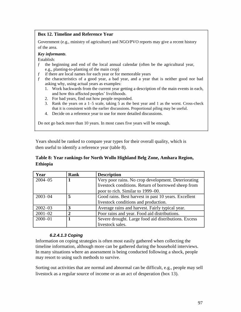
Box 12. Timeline and Reference Year

Government (e.g., ministry of agriculture) and NGO/PVO reports may give a recent history

of the area.

Key informants. Establish: ƒ the beginning and end of the local annual calendar (often be the agricultural year,

e.g., planting-to-planting of the main crop) ƒ if there are local names for each year or for memorable years ƒ the characteristics of a good year, a bad year, and a year that is neither good nor bad

asking why, using actual years as examples: 1. Work backwards from the current year getting a description of the main events in each,

and how this affected peoples’ livelihoods. 2. For bad years, find out how people responded. 3. Rank the years on a 1–5 scale, taking 5 as the best year and 1 as the worst. Cross-check

that it is consistent with the earlier discussions. Proportional piling may be useful. 4. Decide on a reference year to use for more detailed discussions.

Do not go back more than 10 years. In most cases five years will be enough.

Years should be ranked to compare year types for their overall quality, which is

then useful to identify a reference year (table 8). Table 8: Year rankings for North Wollo Highland Belg Zone, Amhara Region,

Ethiopia

Year Rank Description 2004–05 1 Very poor rains. No crop development. Deteriorating

livestock conditions. Return of borrowed sheep from

poor to rich. Similar to 1999–00.

2003–04 5 Good rains. Best harvest in past 10 years. Excellent

livestock conditions and production.

2002–03 3 Average rains and harvest. Fairly typical year.

2001–02 2 Poor rains and year. Food aid distributions. 2000–01 1 Severe drought. Large food aid distributions. Excess

livestock sales.

6.2.4.1.3 Coping

Information on coping strategies is often most easily gathered when collecting the

timeline information, although more can be gathered during the household interviews.

In many situations where an assessment is being conducted following a shock, people

may resort to using such methods to survive. Sorting out activities that are normal and abnormal can be difficult, e.g., people may sell

livestock as a regular source of income or as an act of desperation (box 13).

97

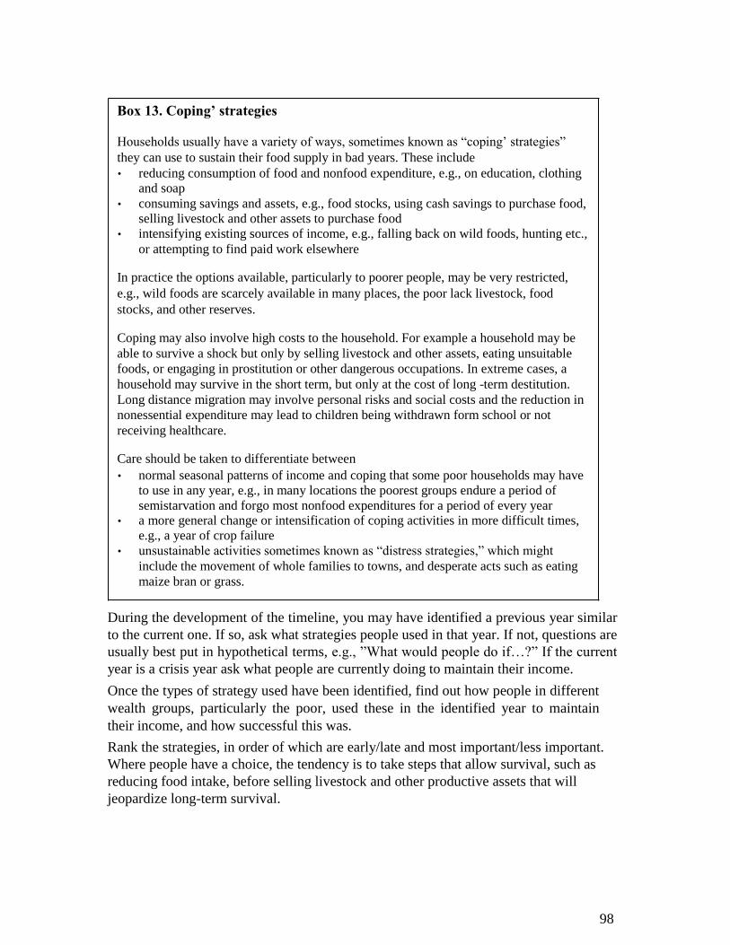
Box 13. Coping’ strategies

Households usually have a variety of ways, sometimes known as “coping’ strategies”

they can use to sustain their food supply in bad years. These include • reducing consumption of food and nonfood expenditure, e.g., on education, clothing

and soap • consuming savings and assets, e.g., food stocks, using cash savings to purchase food,

selling livestock and other assets to purchase food

• intensifying existing sources of income, e.g., falling back on wild foods, hunting etc.,

or attempting to find paid work elsewhere

In practice the options available, particularly to poorer people, may be very restricted,

e.g., wild foods are scarcely available in many places, the poor lack livestock, food

stocks, and other reserves.

Coping may also involve high costs to the household. For example a household may be

able to survive a shock but only by selling livestock and other assets, eating unsuitable

foods, or engaging in prostitution or other dangerous occupations. In extreme cases, a

household may survive in the short term, but only at the cost of long -term destitution.

Long distance migration may involve personal risks and social costs and the reduction in

nonessential expenditure may lead to children being withdrawn form school or not

receiving healthcare.

Care should be taken to differentiate between • normal seasonal patterns of income and coping that some poor households may have

to use in any year, e.g., in many locations the poorest groups endure a period of

semistarvation and forgo most nonfood expenditures for a period of every year • a more general change or intensification of coping activities in more difficult times,

e.g., a year of crop failure • unsustainable activities sometimes known as “distress strategies,” which might

include the movement of whole families to towns, and desperate acts such as eating

maize bran or grass.

During the development of the timeline, you may have identified a previous year similar

to the current one. If so, ask what strategies people used in that year. If not, questions are

usually best put in hypothetical terms, e.g., ”What would people do if…?” If the current

year is a crisis year ask what people are currently doing to maintain their income. Once the types of strategy used have been identified, find out how people in different

wealth groups, particularly the poor, used these in the identified year to maintain

their income, and how successful this was. Rank the strategies, in order of which are early/late and most important/less important.

Where people have a choice, the tendency is to take steps that allow survival, such as

reducing food intake, before selling livestock and other productive assets that will

jeopardize long-term survival.

98

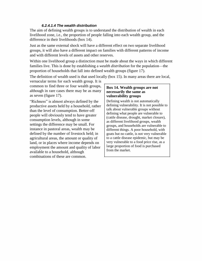
6.2.4.1.4 The wealth distribution The aim of defining wealth groups is to understand the distribution of wealth in each

livelihood zone, i.e., the proportion of people falling into each wealth group, and the

difference in their livelihoods (box 14). Just as the same external shock will have a different effect on two separate livelihood

groups, it will also have a different impact on families with different patterns of income

and with different levels of assets and other reserves. Within one livelihood group a distinction must be made about the ways in which different

families live. This is done by establishing a wealth distribution for the population—the

proportion of households that fall into defined wealth groups (figure 17). The definition of wealth used is that used locally (box 15). In many areas there are local, vernacular terms for each wealth group. It is

common to find three or four wealth groups,

although in rare cases there may be as many

as seven (figure 17). “Richness” is almost always defined by the

productive assets held by a household, rather

than the level of consumption. Better-off

people will obviously tend to have greater

consumption levels, although in some

settings the difference may be small. For

instance in pastoral areas, wealth may be

defined by the number of livestock held; in

agricultural areas, the amount or quality of

land, or in places where income depends on

employment the amount and quality of labor

available to a household, although

combinations of these are common.

Box 14. Wealth groups are not necessarily the same as vulnerability groups

Defining wealth is not automatically defining vulnerability. It is not possible to talk about vulnerable groups without defining what people are vulnerable to (cattle disease, drought, market closure), as different livelihood groups, wealth groups, and households are vulnerable to different things. A poor household, with goats but no cattle, is not very vulnerable to a cattle disease epidemic, but may be very vulnerable to a food price rise, as a large proportion of food is purchased

from the market.

99

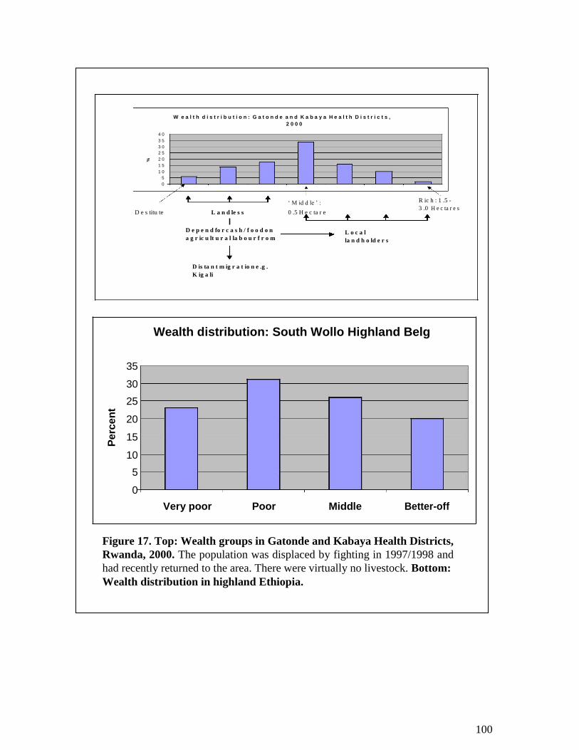
W e a l t h d i s t r i b u t i o n : G a t o n d e a n d K a b a y a H e a l t h D i s t r i c t s ,

2 0 0 0

4 0

3 5

3 0

% 2 5

2 0

1 5

1 0

5

0

‘ M id d le ’ : R ic h : 1 .5 -

D e s titu te

3 .0 H e c ta r e s

L a n d le s s 0 .5 H e c ta r e

D e p e n d fo r c a s h / f o o d o n L o c a l

a g r ic u lt u r a l la b o u r f r o m

la n d h o ld e r s

D is ta n t m ig r a t io n e .g .

K ig a li

Wealth distribution: South Wollo Highland Belg

35

30

Pe

rce

nt

25

20

15

10

5

0

Very poor Poor Middle Better-off

Figure 17. Top: Wealth groups in Gatonde and Kabaya Health Districts,

Rwanda, 2000. The population was displaced by fighting in 1997/1998 and

had recently returned to the area. There were virtually no livestock. Bottom: Wealth distribution in highland Ethiopia.

100

At this stage it is also useful to obtain an estimate of the assets available to each wealth

group, as these often represent a large part of the household’s ability to withstand shocks

(table 9). Tradable assets include livestock holdings (which are the major investment and

reserve in most agricultural and pastoral economies), food stocks, and cash savings.

Table 9: Wealth group characteristics Characteristics Poor Middle Better off

% of Total Population 50%–60% 25%–35% 10%–15%

Land cultivated 1–3 acres 5–7 acres 8–10 acres

Livestock 0–2 cattle 5–10 cattle 15–25 cattle < 5 goats (1–2 milking) (2–3 milking)

10–15 chickens 10–15 goats 20–30 goats

<5 sheep 10–15 sheep

15–20 chickens 15–25 chickens

Household size 6 (1 wife) 6 (1 wife) 11 (2 wives)

Main activities Agricultural labor, Selling livestock, Selling livestock, brewing, selling thatch, brewing, selling selling cotton,

construction, selling thatch, selling brewing, selling

vegetables and wild vegetables, wage vegetables, wage

fruits, crafts employment outside employment outside

district, fishing district

Box 15: Identifying wealth groups This can be a sensitive subject as it concerns wealth (and power). In group discussions avoid

terms such as “the poor” and “the rich.” Find out if there are local terms for wealth groups.

If so, use those. If not, use “better-off” or “worse-off.”

• Find out what makes people better- or worse-off? Land? Cattle? Are some people

more affected by particular shocks, e.g., drought or conflict? • Exclude wealth extremes from the discussion (the destitute, disabled, etc.) and very

rich (e.g., a single landlord, shopkeeper, or other very rich household). You are

interested in the more common and general categories of wealth)

Go through each group identified and establish • the approximate household size and composition of each group • their assets (land, livestock, food stocks, and cash)

• ranges to estimate numbers (e.g., 3–4 cattle owned for most typical households; 1–2

acres planted by most poorer people)

Ask about the relationships between the different groups. Do the poor work for wealthier

households?

Estimate the proportion of the (livelihood group) population in each category.

Proportional piling exercises may be useful if people are unfamiliar with percentages.

101

6.2.4.2 Seasonal Calendar Rural livelihood patterns usually change significantly from season to season. The

availability of many food and income strategies and options is seasonal, as are some

expenditure patterns. Understanding when different sources of income are obtained is

necessary to estimate how needs will vary with the timing of a shock (box 16, figure 18).

Box 16. Seasonal calendar Use flip chart paper or one sheet of paper for each source of food and cash income. Mark the

months down the side. Use local months and the agricultural calendar if this is easier for the

respondents. Establish the main seasons and their characteristics, identifying local names, and

major characteristics (rains, dry, hot, etc.) Income For each main crop and other economic activity in turn, work through month by month

and establish: • crops—the timing of harvests • periods when wild foods (including fishing and hunting) are available • livestock—times when milk is more plentiful, livestock migration, and peak- and low-

sale levels • periods at which the main sources of employment are available, e.g., petty trade,

gathering firewood, construction materials, etc. Ask whether there are particular names or characteristics that are useful and descriptive, such

as “the hunger season” or “the time of plenty.” Expenditure • seasonal pattern of food purchase and other major expenditures—water, agricultural

inputs, schooling: • 0rices of main commodities purchased and sold Draw these patterns on a simple annual calendar

102

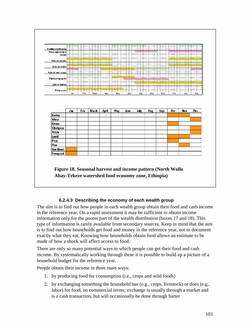
Figure 18. Seasonal harvest and income pattern (North Wollo

Abay-Tekeze watershed food economy zone, Ethiopia)

6.2.4.3 Describing the economy of each wealth group

The aim is to find out how people in each wealth group obtain their food and cash income

in the reference year. On a rapid assessment it may be sufficient to obtain income

information only for the poorer part of the wealth distribution (boxes 17 and 18). This

type of information is rarely available from secondary sources. Keep in mind that the aim

is to find out how households get food and money in the reference year, not to document

exactly what they eat. Knowing how households obtain food allows an estimate to be

made of how a shock will affect access to food. There are only so many potential ways in which people can get their food and cash

income. By systematically working through these it is possible to build up a picture of a

household budget for the reference year. People obtain their income in three main ways:

1. by producing food for consumption (i.e., crops and wild foods)

2. by exchanging something the household has (e.g., crops, livestock) or does (e.g.,

labor) for food, on commercial terms; exchange is usually through a market and

is a cash transaction, but will occasionally be done through barter

103

3. as gifts, i.e., flows of food, money (and occasionally livestock and other goods)

on broadly nonmarket terms; gifts may be just that (e.g., free relief food) or

involve some return from the recipient (e.g., some token work or the expectation

that the gift will be returned at some future time when the giver is in need)

Box 17. Describing the economy I

Before starting discussion be sure that you know the types of income obtained in the livelihood

group, the seasonality of crop, employment, and wild food income. The informant should be

someone who has a close knowledge of village economy, i.e., someone from a village.

Work systematically through the three production categories

• crops produced by the household

• livestock and livestock products (milk, meat, eggs, blood) produced by the household

• wild foods/hunting.

Then work through the five exchange categories:

• crop sales (including cash crops such as cotton or tobacco or the sale of food crops

• sale of livestock and livestock products

• wild food sales

• labor sales, subdivided into paid employment (e.g., agricultural labour, government

service), self-employment (e.g., firewood, charcoal, handicrafts, transport, and resale of

goods/petty trade, remittance, etc.), and gifts (of food or cash) and gift sales (e.g., of

relief food)

How people—particularly very poor people—use these options is not always

straightforward. For example, people may sell food crops after the harvest to get cash to

pay school fees, then have to buy food from the market later in the year, often at a

higher price. However, for a rapid assessment, all you need to know is how much

income the household obtained from different sources in the reference year. This information is obtained by systematically working through the production and

exchange headings (see boxes 17 and 18) with an informant to get an estimate of the

income from each source. From the previous steps and before the start of this discussion

you should already have identified the wealth groups and their assets; and know the

potential sources of income for the livelihood group, the seasonality of each, and about

coping strategies in bad years. 104

6.2.4.4 Note for describing economies

6.2.4.4.1 Units People do not always work in metric or other conventional units. Imperial units (e.g., acres,

pounds) may be used, traditional units (e.g., maunds), or bags, cups, tins, pails, and other

local units. Local units should be used in recording the quantity of income obtained. As units

will have to be converted to metric units for the analysis, it is important to ensure that their

metric equivalents are known. It is often the case that key informants know the metric

equivalents, at least of the main marketed crops. Bags are typically 50kg. It may be possible

to calculate other volumetric units from this (e.g., if it is known that, for a particular crop 5

pails = 1 bag, 8 bags = 1 oxcart). Otherwise the quantity concerned must be weighed.

Bundles, bales, etc., may have a metric weight equivalent (as for cotton). Otherwise, ensure

that the price of one bundle (or bale) is known. For items that involve a large amount of processing waste, take care to specify

whether the item is processed or unprocessed, e.g., groundouts may be reported as

shelled or unshelled.

Box 18. Describing the economy II

Secondary sources are not always available or reliable and do not often have information

in the format required here. From the previous discussions a qualitative description of

the main features of the economy is available, i.e., the main crops produced, harvest

times, types of paid employment and self-employment, wild foods etc.

All that is required is to work systematically, wealth group by wealth group, through

the main income headings, to build up a picture of the pattern of income of each group.

Ensure that the informant is clear about

• which wealth group (“poor,” “middle”) is under discussion

• the discussion referring to the reference year

• the size of the household under discussion

• using local units, e.g., bags, tins

Work though each source of food and cash income in turn to quantify it and establish its

relative importance to that wealth group.

If time allows, repeat the discussion at other representative sites.

6.2.4.4.2 Minor income sources

On a rapid assessment do not dwell on very small sources of income. For instance, a

variety of types of wild fruits are eaten in many places. These are often of very low

energy value, and highly seasonal. If it is clear these cannot be more than a very small

proportion of income, they can be ignored (box 19). Children, particularly boys, are often

partly “self–provisioning” (they may obtain small jobs for food, hunt, and consume small

birds and other animals), but in the context of a rapid assessment, the contribution to

household income is often very small.

105

Paid and self-employment Employment is often highly seasonal, following the pattern of agriculture, or— particularly

off-season—taken piecemeal as the opportunity arises. Wage rates may vary seasonally and be different for

men and women. Work through

each employment type month by

month, for men and women

separately if necessary, and find

out approximately how many

days employment is obtained in

each month.

6.2.4.4.2.2 Remittances Ask if there are people working

outside the village, and if so,

where they are working, how

much time they are away, and the contribution that they make to household income. In some cases it will be found that

remittances from workers overseas will be among the largest income sources.

6.2.4.5 For how many wealth groups should information be obtained?

The aim of a rapid assessment is usually to determine the ability of the poorest groups

to acquire sufficient food. If time allows, try to get information for at least three groups.

Of course, where there are a large number of wealth groups, it would be impractical to

obtain information on all. However, sufficient groups should be included to provide a

representation of the whole population, i.e., a poor, middle, and better-off group. Or, if

time is limited, ensure that information is obtained at least for the poorest and middle

groups—those most likely to be in difficulty.

6.2.4.6 Standard of living Lastly some information will be required on the nonfood costs of maintaining a basic

standard of living. Typically this would include • personal costs, i.e., clothing, soap (personal and clothes washing) • household items, i.e., fuel (often a small amount of kerosene or diesel used

for lighting), cooking utensils • education costs (even if no direct charge is made for school there are costs for books,

examination fees, etc.

• health costs 53

53

as health costs vary a great deal from household to household, a reasonable compromise is to add an

amount sufficient to meet the costs of basic routine care, e.g., transport costs for immunization, 1–2 clinic

visits by each child per year, including transport costs and, where relevant, user fees, and drug costs.

106

Box 19. “Appropriate imprecision”

The precision of the estimates depends on the intended use of the data. In a rapid food security assessment the usual aim is to understand the impact of a gross change, e.g., major drought or crop loss, collapse of employment on economy, usually on people who already live on an economic edge. Under these conditions the omission of small items of income and the use of approximations is unlikely to make much

difference to the analysis.

It will often be found that the actual nonfood expenditure of the poorest groups will

fall below even the most basic standard of living, at least seasonally.

6.2.4.6.1 Common difficulties

Knowing if the information obtained is reliable. This can be checked in two main ways:

1. Household income should be at a

level consistent with household

food needs. During an interview,

keep a running account of income

sources as you go along to ensure

that the food income (including

food purchase) adds up to a

quantity consistent with household

needs, and that the cash left over is

consistent with the observed

standard of living. It is helpful to

memorize the approximate quantities of staple foods that are required by a defined household, e.g., a

household of five will use approximately a ton of cereals (20 bags of 50kg) a year

(box 20) and the approximate nonfood costs of a household in that wealth group.

2. More than one key informant discussion should be held for each wealth group to

triangulate the findings. The findings from different interviews should be

reasonably consistent. Occasional income sources, e.g., fishing, might be classified under different headings.

For example, sea or river fish might fall under hunting; fish farming under livestock; and

mango trees may be semi- wild or private property. For a rapid assessment either

classification will do, as it makes no difference to the analysis. The important thing is to

ensure that all major sources of income are included.

6.2.5 Defining the shock In understanding people’s food security, it is necessary to define the shock that has

occurred, in terms of its relationship to people’s sources of food and income. For

instance, cereal production may be reduced for a variety of reasons, e.g., drought, flood,

or transport failure. Whatever the immediate cause, the shock is defined as the actual

impact this has had on production and/or prices, as it is this that affects the food

security of people in the defined livelihood groups (box 21). The way in which a shock has affected the economy can be estimated in two ways: • Official sources may sometimes be helpful for estimating crop production, although

official crop statistics are often reported with respect to administrative rather than

livelihood zones and are not always available until some time after the event. Local

agricultural extension officers are often good key informants and may have a good

overview of an area. It is rare for official statistics for current livestock production,

employment or other sources of income to be available at all.

107

For relief calculations an average of 2,100kcal per person per day is often used. A household of five would require 5 x 2,100 x 365kcal/year = 3,832,500kcal/year. In many areas the actual food intake of poorer household is often less than this. An average of 1,800kcal/person/day is not an unusual finding.

Box 20. Food energy needs

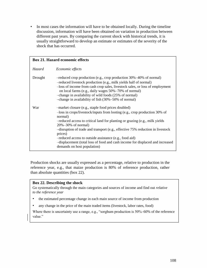
• In most cases the information will have to be obtained locally. During the timeline

discussion, information will have been obtained on variation in production between

different past years. By comparing the current shock with historical trends, it is

usually straightforward to develop an estimate or estimates of the severity of the

shock that has occurred.

Box 21. Hazard economic effects

Hazard Economic effects

Drought –reduced crop production (e.g., crop production 30%–40% of normal)

–reduced livestock production (e.g., milk yields half of normal) –loss of income from cash crop sales, livestock sales, or loss of employment

on local farms (e.g., daily wages 50%–70% of normal) –change in availability of wild foods (25% of normal) –change in availability of fish (30%–50% of normal)

War –market closure (e.g., staple food prices doubled)

–loss in crops/livestock/inputs from looting (e.g., crop production 30% of normal) –reduced access to critical land for planting or grazing (e.g., milk yields 20%–30% of normal) –disruption of trade and transport (e.g., effective 75% reduction in livestock prices) –reduced access to outside assistance (e.g., food aid) –displacement (total loss of food and cash income for displaced and increased demands on host population)

Production shocks are usually expressed as a percentage, relative to production in the

reference year, e.g., that maize production is 80% of reference production, rather

than absolute quantities (box 22).

Box 22. Describing the shock Go systematically through the main categories and sources of income and find out relative

to the reference year • the estimated percentage change in each main source of income from production

• any change in the price of the main traded items (livestock, labor rates, food)

Where there is uncertainty use a range, e.g., “sorghum production is 50%–60% of the reference

value.”

108

6.2.5.1 Common difficulties 1. If the rate of price inflation is very high (e.g., as sometimes happens in war

zones), the cost of food or other items may appear to have risen, even over 1–2

years, when in fact it has not. The true change in value of a commodity can be

established by looking at the relative value of different items.

2. A range of estimates may be obtained from different sources. Record any

variation in the form of ranges e.g., sorghum prices increased by 30%–40%, or

production is only 70%–90% of (or 10%–30% below) that in the reference year.

6.3 Estimating the impact of a shock on food access:

Putting nutritional survey results in context Box 23 discusses analysis for predicting the impact of a shock.

Box 23. Prediction

Where an analysis has been made to predict the impact of a shock, e.g., an anticipated

harvest failure, before people have had to compensate for reduced income, an analysis

requires decisions on the following:

• The proportion of any assets that the population should be allowed to retain. For

example, if a wealth-group household has 10 goats, how many should the household

be “allowed” to sell? For the poorest groups, the decision is often made easy by the

fact that the asset base is often so small that it can be ignored (table 5). Land,

agricultural tools, household furniture, and the other basic requirements for long-term

subsistence should not be included if the sale of these would be necessary to survival.

Wild foods should be included only in the (now rare) case that these are readily

available, nutritionally useful, and do not require extraordinary processing to make

edible; and long-distance migration takes place only if this is not unduly hazardous. • What is an acceptable level of nonfood consumption, e.g., soap and clothing. If no

allowance is made for this, food (e.g., food aid) will be sold to purchase essentials, and

food intake will be reduced. 6.3.1 Steps in conducting an analysis A worked example is given in the next section. The steps are as follows:

1. Calculate the amount and proportion of income that each household type/wealth

group obtains from each food and cash income source.

2. Combine the income and the seasonality information to develop a timeline to

“explain” how food access has changed in the period before the survey, and to

project this into the future. This can then be compared with the nutrition findings. The way in which this is done will depend on the time at which the food security

assessment is being done relative to the shock. There are broadly two situations:

109

1. Where an assessment has been done after a food security problem has already

arisen, people will have already adjusted to the crisis to the extent possible, e.g.,

sold assets and consumed other reserves. This is the most common situation

where anthropometry is undertaken. This situation is used is used as the basis for

discussion.

2. Where an assessment is being conducted with the aim of predicting the effect of a

shock (e.g., a crop failure has occurred and the need is to know how food security

is likely to evolve in future), there may be an opportunity to take action before

food access and nutritional status fall. In this case, analysis requires some further

judgments to be made (box 23). The calculations required are simple but the numbers can become large, and it is easy to

make errors. The calculations are most easily done using a spreadsheet. Where there is

doubt about the value of some variables, a spreadsheet also allows several scenarios to be

tested quickly. For instance, if the estimate of crop production in the current year is in the

range of 60%–70% of reference year production, analyses can be done using the lower

and higher estimate. A spreadsheet (SMART_FOOD_SECURITY_CALCULATOR.xls) is provided with

this manual. This has three worksheets:

1. A simple calculator that allows the household budget data to be entered reconciled

and checked.

2. For the entry of seasonal information e.g., the percentage of a particular crop that

is harvested in a particular month.

3. Calculates the expected food access of each wealth group, under

conditions specified by the user. The spreadsheet allows an analysis to be done for a livelihood zone with up to four

wealth groups. The spreadsheet is supplied with data for a livelihood zone already

entered. An additional copy of the spreadsheet should be made for each new livelihood

zone to be entered.

6.3.2 Step 1: Worksheet 1. Calculating the amount of income

obtained from each income source

Worksheet cells in which data is to be entered by the user is in blue (figure 19). Values in

black are calculated automatically by the spreadsheet. For each wealth group enter the

following:

1. Wealth group name, proportion of the population in each wealth group, number

of people in the household, and food energy requirement/person/day.

2. Name of each income source, food energy values (see annex 2), and/or price

of any traded item. Any units of income, e.g., bags, can be used as long as

appropriate food energy and price values are used.

3. Reference values (quantity of income obtained from each source for each wealth

group). The calculations will be done automatically. 110

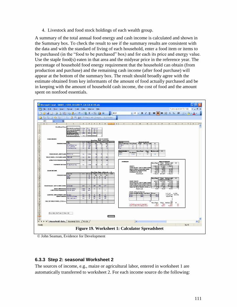
4. Livestock and food stock holdings of each wealth group. A summary of the total annual food energy and cash income is calculated and shown in

the Summary box. To check the result to see if the summary results are consistent with

the data and with the standard of living of each household, enter a food item or items to

be purchased (in the “food to be purchased” box) and for each its price and energy value.

Use the staple food(s) eaten in that area and the midyear price in the reference year. The

percentage of household food energy requirement that the household can obtain (from

production and purchase) and the remaining cash income (after food purchase) will

appear at the bottom of the summary box. The result should broadly agree with the

estimate obtained from key informants of the amount of food actually purchased and be

in keeping with the amount of household cash income, the cost of food and the amount

spent on nonfood essentials.

Figure 19. Worksheet 1: Calculator Spreadsheet

© John Seaman, Evidence for Development

6.3.3 Step 2: seasonal Worksheet 2 The sources of income, e.g., maize or agricultural labor, entered in worksheet 1 are

automatically transferred to worksheet 2. For each income source do the following: 111

1. Enter the percentage of each income source obtained in the appropriate month

column. For example, if the maize harvest is in March and April, with most of

the crop obtained in April, the entries might be March 30%, April 70%. Note that

the entries should add up to 100%. The total for each row is shown in the column

on the right.

2. Enter a nonfood cost/household (at the bottom left of the seasonality section).

The nonfood cost should represent the cost of a reasonable basic standard of

living (section 1.2.4.6, the standard of living). The monthly nonfood cost will be

calculated automatically

6.3.4 Putting the shock information and the economic description together

to develop a food security narrative Step 3: Worksheet 3, the model Worksheet 3 calculates the percentage of household food requirement that each household can obtain, from its own production and food purchase month by month over

a two-year period, given a set of conditions specified by the user. 54

The conditions that

can be set include the level of production and income from different sources, food prices, the quantity of nonfood items that the household will purchase, and the extent to which a household can “cope” by selling livestock and other steps. Taken together these can be used to simulate the effect of a shock on household food access. The conditions are set in the top part of worksheet 3. Year 1 will usually include some or all of the most recent past year up to the point of the nutrition assessment. Part of year 1 and year 2 will be a forward projection from that point. The changes that can be made are as follows:

1. The level of production or income set for each of the two years, expressed as a

percentage of the reference income. For example, if drought caused a fall maize

production to 50% of reference values, 50% would be entered in the relevant

cell for year 1. The value for year 2 will be unknown. However it is possible to

enter conjectural values for year 2 to allow the development of hypothetical

scenarios. For instance, how would the situation be likely to develop if the

harvest in year 2 were normal or only 80% of normal?

2. The price that people had to/ will have to pay to purchase food. The foods

specified should be the cheapest available staple foods consistent with the

reasonable survival of the people in the livelihood zone. A diet of up to four items

can be entered, although in many situations one (a staple) or two items will

suffice. In the spreadsheet example, the diet has been specified as 90% maize and

10% beans. The price of each item is entered for each month for each of the three

54

This calculates 1) the amount of food available from production for each month in the reference year,

year 1 and year 2, given the percentages of income set by the user; 2) the amount of food that a household

would have to purchase each month to make up its requirement, allowing for carry-over between months

e.g., production income tends to be concentrated in a few months; 3) nonfood and food expenditure is

calculated, again allowing for carry-over of unspent cash between months. Year 1 begins with the starting

values of the reference year i.e., it assumes a reference year preceding year 1. Year 2 begins with the output

from year 1. “Coping” income, if set, is added in January of years 1 and 2.

112

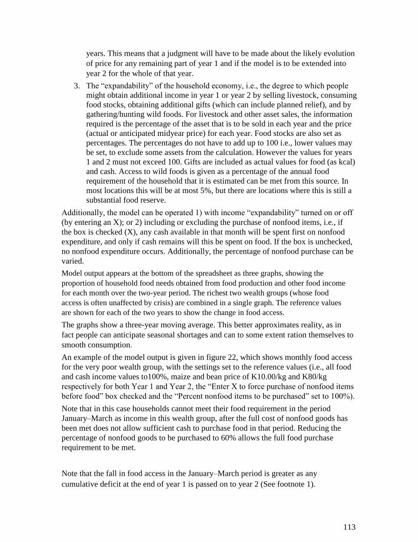
years. This means that a judgment will have to be made about the likely evolution

of price for any remaining part of year 1 and if the model is to be extended into

year 2 for the whole of that year.

3. The “expandability” of the household economy, i.e., the degree to which people

might obtain additional income in year 1 or year 2 by selling livestock, consuming

food stocks, obtaining additional gifts (which can include planned relief), and by

gathering/hunting wild foods. For livestock and other asset sales, the information

required is the percentage of the asset that is to be sold in each year and the price

(actual or anticipated midyear price) for each year. Food stocks are also set as

percentages. The percentages do not have to add up to 100 i.e., lower values may

be set, to exclude some assets from the calculation. However the values for years

1 and 2 must not exceed 100. Gifts are included as actual values for food (as kcal)

and cash. Access to wild foods is given as a percentage of the annual food

requirement of the household that it is estimated can be met from this source. In

most locations this will be at most 5%, but there are locations where this is still a

substantial food reserve. Additionally, the model can be operated 1) with income “expandability” turned on or off

(by entering an X); or 2) including or excluding the purchase of nonfood items, i.e., if

the box is checked (X), any cash available in that month will be spent first on nonfood

expenditure, and only if cash remains will this be spent on food. If the box is unchecked,

no nonfood expenditure occurs. Additionally, the percentage of nonfood purchase can be

varied. Model output appears at the bottom of the spreadsheet as three graphs, showing the

proportion of household food needs obtained from food production and other food income

for each month over the two-year period. The richest two wealth groups (whose food

access is often unaffected by crisis) are combined in a single graph. The reference values

are shown for each of the two years to show the change in food access. The graphs show a three-year moving average. This better approximates reality, as in

fact people can anticipate seasonal shortages and can to some extent ration themselves to

smooth consumption. An example of the model output is given in figure 22, which shows monthly food access

for the very poor wealth group, with the settings set to the reference values (i.e., all food

and cash income values to100%, maize and bean price of K10.00/kg and K80/kg

respectively for both Year 1 and Year 2, the “Enter X to force purchase of nonfood items

before food” box checked and the “Percent nonfood items to be purchased” set to 100%). Note that in this case households cannot meet their food requirement in the period

January–March as income in this wealth group, after the full cost of nonfood goods has

been met does not allow sufficient cash to purchase food in that period. Reducing the

percentage of nonfood goods to be purchased to 60% allows the full food purchase

requirement to be met. Note that the fall in food access in the January–March period is greater as any

cumulative deficit at the end of year 1 is passed on to year 2 (See footnote 1).

113

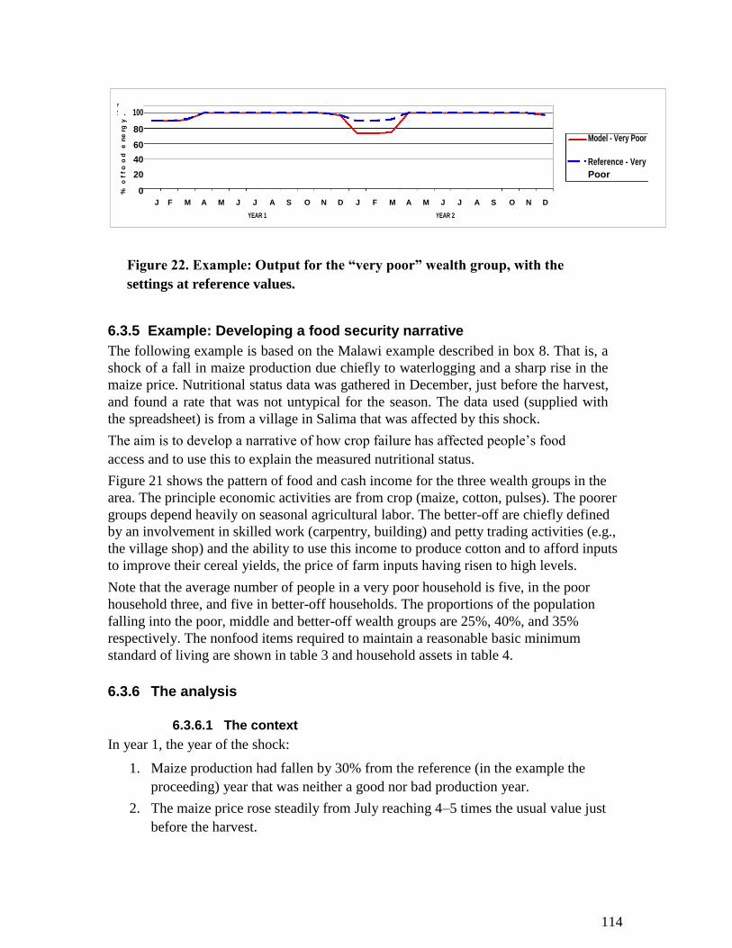
re q

. 100

y

80

n

e r

g

Model - Very Poor

60

e

o d

40 Reference - Very

f f

o

20 Poor

o

0

%

F M A M J J A S O N D J F M A M J J A S O N D

J

YEAR 1 YEAR 2

Figure 22. Example: Output for the “very poor” wealth group, with the

settings at reference values.

6.3.5 Example: Developing a food security narrative The following example is based on the Malawi example described in box 8. That is, a

shock of a fall in maize production due chiefly to waterlogging and a sharp rise in the

maize price. Nutritional status data was gathered in December, just before the harvest,

and found a rate that was not untypical for the season. The data used (supplied with

the spreadsheet) is from a village in Salima that was affected by this shock. The aim is to develop a narrative of how crop failure has affected people’s food

access and to use this to explain the measured nutritional status. Figure 21 shows the pattern of food and cash income for the three wealth groups in the

area. The principle economic activities are from crop (maize, cotton, pulses). The poorer

groups depend heavily on seasonal agricultural labor. The better-off are chiefly defined

by an involvement in skilled work (carpentry, building) and petty trading activities (e.g.,

the village shop) and the ability to use this income to produce cotton and to afford inputs

to improve their cereal yields, the price of farm inputs having risen to high levels. Note that the average number of people in a very poor household is five, in the poor

household three, and five in better-off households. The proportions of the population

falling into the poor, middle and better-off wealth groups are 25%, 40%, and 35%

respectively. The nonfood items required to maintain a reasonable basic minimum

standard of living are shown in table 3 and household assets in table 4.

6.3.6 The analysis

6.3.6.1 The context

In year 1, the year of the shock:

1. Maize production had fallen by 30% from the reference (in the example the

proceeding) year that was neither a good nor bad production year.

2. The maize price rose steadily from July reaching 4–5 times the usual value just

before the harvest. 114

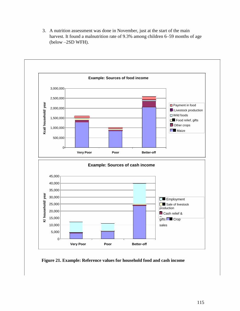
3. A nutrition assessment was done in November, just at the start of the main

harvest. It found a malnutrition rate of 9.3% among children 6–59 months of age

(below –2SD WFH).

Example: Sources of food income

3,000,000

2,500,000

ye

ar

2,000,000

ho

us

eh

old

/

1,500,000

1,000,000

Kc

al/

500,000

0

Very Poor Poor Better-off

Payment in food Livestock production

Wild foods Food relief, gifts

Other crops

Maize

Example: Sources of cash income

45,000

40,000

ye

ar

35,000

30,000

ho

us

eh

old

/

25,000

20,000

15,000

K/

10,000

5,000

0

Very Poor Poor Better-off

Employment Sale of livestock

production Cash relief &

gifts Crop

sales

Figure 21. Example: Reference values for household food and cash income 115

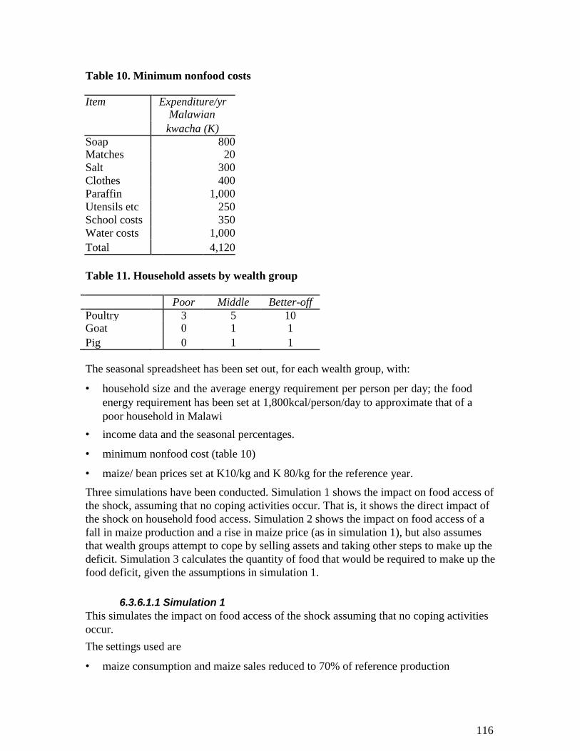
Table 10. Minimum nonfood costs

Item Expenditure/yr

Malawian

kwacha (K)

Soap 800

Matches 20

Salt 300

Clothes 400

Paraffin 1,000

Utensils etc 250

School costs 350

Water costs 1,000

Total 4,120

Table 11. Household assets by wealth group

Poor Middle Better-off

Poultry 3 5 10 Goat 0 1 1

Pig 0 1 1

The seasonal spreadsheet has been set out, for each wealth group, with:

• household size and the average energy requirement per person per day; the food

energy requirement has been set at 1,800kcal/person/day to approximate that of a

poor household in Malawi • income data and the seasonal percentages.

• minimum nonfood cost (table 10)

• maize/ bean prices set at K10/kg and K 80/kg for the reference year.

Three simulations have been conducted. Simulation 1 shows the impact on food access of

the shock, assuming that no coping activities occur. That is, it shows the direct impact of

the shock on household food access. Simulation 2 shows the impact on food access of a

fall in maize production and a rise in maize price (as in simulation 1), but also assumes

that wealth groups attempt to cope by selling assets and taking other steps to make up the

deficit. Simulation 3 calculates the quantity of food that would be required to make up the

food deficit, given the assumptions in simulation 1.

6.3.6.1.1 Simulation 1 This simulates the impact on food access of the shock assuming that no coping activities

occur. The settings used are

• maize consumption and maize sales reduced to 70% of reference production

116

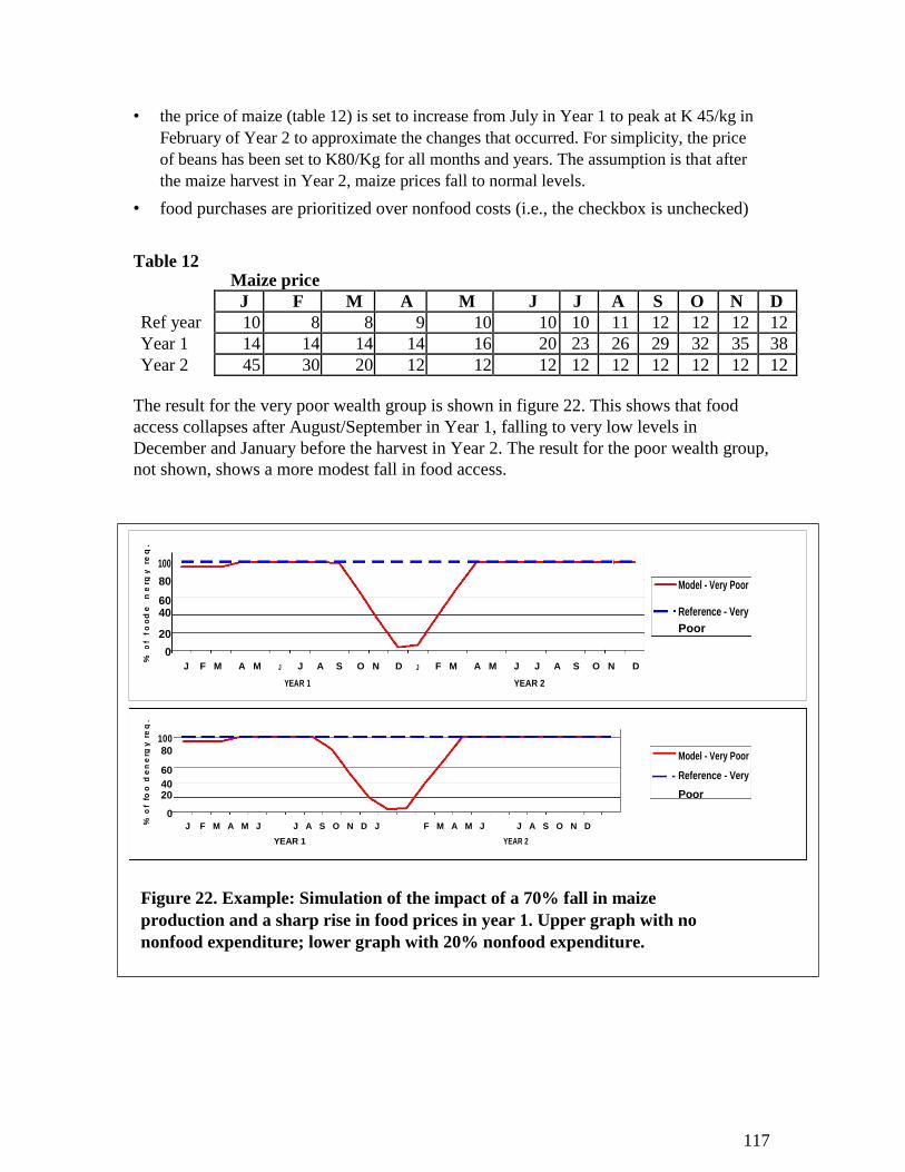
• the price of maize (table 12) is set to increase from July in Year 1 to peak at K 45/kg in

February of Year 2 to approximate the changes that occurred. For simplicity, the price

of beans has been set to K80/Kg for all months and years. The assumption is that after

the maize harvest in Year 2, maize prices fall to normal levels. • food purchases are prioritized over nonfood costs (i.e., the checkbox is unchecked)

Table 12 Maize price

Ref year

J F M A M J J A S O N D

10 8 8 9 10 10 10 11 12 12 12 12

Year 1 14 14 14 14 16 20 23 26 29 32 35 38

Year 2 45 30 20 12 12 12 12 12 12 12 12 12

The result for the very poor wealth group is shown in figure 22. This shows that food

access collapses after August/September in Year 1, falling to very low levels in

December and January before the harvest in Year 2. The result for the poor wealth group,

not shown, shows a more modest fall in food access.

re q

.

100

y

80

e r

g

Model - Very Poor

n

60

d e

Reference - Very

40

f o

o

20 Poor

o f

0

%

J F M A M J J A S O N D J F M A M J J A S O N D

YEAR 1 YEAR 2

re q

.

100

rg y

80 Model - Very Poor

e

n

60

d e

Reference - Very

40

fo o

Poor

20

o f

0

%

J F M A M J J A S O N D J F M A M J J A S O N D

YEAR 1 YEAR 2

Figure 22. Example: Simulation of the impact of a 70% fall in maize

production and a sharp rise in food prices in year 1. Upper graph with no

nonfood expenditure; lower graph with 20% nonfood expenditure.

117

6.3.6.1.2 Simulation 2 This simulation estimates the impact on food access of a fall in maize production and a

rise in maize price (as in simulation 1), but additionally assumes that wealth groups

attempt to ‘cope ‘ by selling assets and taking other steps to cover the deficit. The settings used (‘Expandability’, worksheet 3) are: • Livestock: 100% to be sold in year 1. As many people are attempting to sell livestock,

livestock prices would be expected to fall. In fact, livestock prices fell and maize

prices rose to the point where people ate the animals rather than sell them.55

For

illustration, it has been assumed that livestock values are maintained at reference values (poultry K75 each, and pigs and goats approximately K1,500 each).

• Food stocks are set at 100% to be consumed. • Gift giving between households tends to collapse under these conditions, and this

value has been set to zero. • Wild foods (chiefly seasonal wild fruits and leaves) make up only 0.9% of the

reference energy requirement of the very poor group. As it would be expected

that demand for wild foods would rise following the shock this has been set to

0.5% of household energy requirement. In fact, in this case people sold not only livestock but also furniture and any goods

for which they could get a price. These have not been factored in to the analysis as

their value is so low.

y r

eq

. 100

en

erg

80

60

d

40

fo

o

20

o f

0

%

J F M A M J J A S O N D J F M A M J J A S O N D

YEAR 1 YEAR 2

Model - Very Poor Reference - Very Poor

Figure 23. Simulation 2. Simulation of the impact of a 70% fall in maize

production and a sharp rise in food prices in year 1, using all coping

strategies and assuming no nonfood expenditure. Figure 23 shows the simulation result, assuming no nonfood expenditure. This suggests

that for the very poor wealth group, the use of all their reserves, even making optimistic

assumptions about the value of these is very small i.e., compare the result with the

upper graph in Figure 22.

55

This could be factored in by calculating the energy value of a goat and adding this to the ‘gift’ section.

118

6.3.6.1.3 Simulation 3 Other statistics can be derived from the model. For example assuming that some

population statistics are available the quantity of maize required to make up the deficit

can be calculated by: • setting a value for nonfood expenditure i.e., a value that is thought under the

circumstances to be commensurate with an acceptable standard of living (50% has

been entered) • setting the coping box to X. • adding values to the food gift section until food access in year 1 approximates the

reference value (in this case for the very poor group, approximately

1,000,000kcal would be required, or 275kg of maize) The number of households in this village was 211, i.e., the very poor group (52

households), suggesting a deficit equivalent to approximately 14 tons.

6.3.6.2 Projecting forward from the nutrition survey

In planning a relief intervention, it is necessary to predict what is going to happen to

people’s food access. This requires an estimate of what is likely to happen to

1. each income source over the coming year

2. the price of traded goods and services

3. possible additional income from government/national and external

intervention, e.g., food aid It is impossible to estimate these with complete confidence. Nevertheless it is possible to

make well-informed judgments.

1. Take each income source in turn and ask if there are any local implications of the

current situation that would argue for a change in income from that source in the

coming year. Discussion with local key informants is usually the best guide to

this. For example, income from crops and local agricultural/unskilled employment

may fall. In the Malawi case, much unskilled labor outside the agricultural season

is found in house building for the better off groups—an activity that occurs only

in years when income is good. In the year following a crisis people, including the

better off, may have difficulty in finding the resources to meet the cost of farm

inputs (fertilizer/pesticides and labor).

2. Where a crisis has had a wider national or regional impact, work and trading

opportunities may fall in a wider area that will reduce employment opportunities,

e.g., on plantations, in cities, and for some, goods and services provided to the

poor.

3. Some assessment must be made of the likelihood of government/national and

external intervention and when and how this will occur. For example, in Malawi,

it was clear at the time of the nutrition assessment that food aid in substantial

quantities would not be available for several months. Malawi is landlocked, and

food would have to be imported and transported over long distances. 119

Uncertainties will remain; for example, it cannot be known if rainfall will be adequate in

the coming year. In cases where there is doubt about factors that may have a major

impact on household economy, more than one scenario can be developed using different

values for each. This allows a range of possible outcomes to be developed and alternative

and fall-back interventions developed for each.

6.3.7 Connecting the food security analysis and nutritional survey

findings. It is not possible to draw a precise connection between household food access and

nutritional status, e.g., that a fall in food access to X% of usual consumption for a given

period will lead to a Y% change in children’s nutrition status. It is not known how food is

distributed within the household, and even if this were known, not enough is known

about individual requirement to make precise calculations. Nevertheless, it would be

expected that large changes in food access will be followed by changes in population

nutritional status, particularly for the poorest people. These groups already have low

energy intakes, low biological reserves and often suffer seasonal falls in food access even

in non-crisis years. Trends in food access can therefore provide a good general guide to

the way in which nutritional status will evolve.

120

7 Interpretation and recommendations This section will be completed in Version 2, based on the experience of

implementing Version 1. 121

122

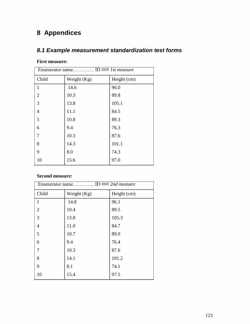
8 Appendices

8.1 Example measurement standardization test forms First measure:

Enumerator name…………. ID ### 1st measure

Child Weight (Kg) Height (cm)

1 14.6 96.0

2 10.3 89.8

3 13.8 105.1

4 11.1 84.5

5 10.8 89.3

6 9.4 76.3

7 10.3 87.6

8 14.3 101.1

9 8.0 74.3

10 15.6 97.0

Second measure:

Enumerator name…………. ID ### 2nd measure

Child Weight (Kg) Height (cm)

1 14.8 96.1

2 10.4 89.5

3 13.8 105.3

4 11.0 84.7

5 10.7 89.0

6 9.4 76.4

7 10.3 87.6

8 14.1 101.2

9 8.1 74.1

10 15.4 97.5

123

8.2 Energy values of foods

This summary table of food energy values has been extracted from Tables of Representative

Values of Foods Commonly Used in Tropical Countries (Platt, 1985). The table is useful for

evaluating dietary data based on records of group consumption. The tables are not suitable for

detailed surveys of the diets of individuals. Food energy values are given as the amount per 100 g

of edible portion.

CEREALS 1. Barley, whole, de-husked 339 2. Barley, pearled 351 3. Buckwheat flour, 90% extraction 348 4. Buckwheat flour, 60% extraction 349 5. Maize, whole 363 6. Maize meal, about 96% extraction 362 7. Maize meal, refined, 60% extraction 354 8. Maize starch (commercial), corn-flour 352 9. Millet, bulrush, whole grains 363 10. Millet, bulrush, meal 365 11. Millet, finger, whole grain 336 12. Millet, finger, meal 332 13. Millet, haraka, de-husked 353 14. Millet, jajeo, de-husked 355 15. Millet, various, de-husked 355 16. Quinoa 345 17. Oats de-husked 388 18. Rice, lightly milled and parboiled 354 19. Rice, highly milled, polished 352 20. Rye, 85-90% extraction 350 21. Sorghum, whole grain 355 22. Sorghum flour 353 23. Teff, whole grains 345 24. Wheat, whole and parboiled 344 25. Wheat flour, 85% extraction 346 26. Wheat flour, 70% extraction 350 STARCHY ROOTS, TUBERS AND FRUITS 27. Arrowroot flour 340 28. Breadfruit pulp 113 29. Cassava, fresh 153 30. Cassava flour 342 31. Ensete 190 32. Plantain 128 33. Potato, Irish 75 34. Potato, Sweet 114 35. Sago flour 352 36. Taro 113 37. Yam, fresh 104 38. Yam flour 317 39. Yam bean tuber 41 OIL SEEDS AND NUTS

124

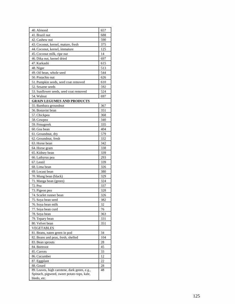
40. Almond 657 41. Brazil nut 688 42. Cashew nut 590 43. Coconut, kernel, mature, fresh 375 44. Coconut, kernel, immature 125 45. Coconut milk, ripe nut 14 46. Dika nut, kernel dried 697 47. Karkashi 615 48. Niger 513 49. Oil bean, whole seed 544 50. Pistachio nut 626 51. Pumpkin seeds, seed coat removed 610 52. Sesame seeds 592 53. Sunflower seeds, seed coat removed 524 54. Walnut 697 GRAIN LEGUMES AND PRODUCTS

55. Bambara groundnut 367 56. Bonavist bean 351 57. Chickpea 368 58. Cowpea 340 59. Fenugreek 335 60. Goa bean 404 61. Groundnut, dry 579 62. Groundnut, fresh 332 63. Horse bean 342 64. Horse gram 338 65. Kidney bean 339 66. Lathyrus pea 293 67. Lentil 339 68. Lima bean 326 69. Locust bean 380 70. Mung bean (black) 329 71. Manga bean (green) 324 72. Pea 337 73. Pigeon pea 328 74. Scarlet runner bean 326 75. Soya bean seed 382 76. Soya bean milk 32 77. Soya bean curd 76 78. Soya bean 363 79. Tepary bean 331 80. Velvet bean 351 VEGETABLES

81. Beans, eaten green in pod 34 82. Beans and peas, fresh, shelled 104 83. Bean sprouts 28 84. Beetroot 45 85. Carrots 33 86. Cucumber 12 87. Eggplant 22 88. Gourd 28 89. Leaves, high carotene, dark green, e.g., 48 Spinach, pigweed, sweet potato tops, kale,

bledo, etc.

125

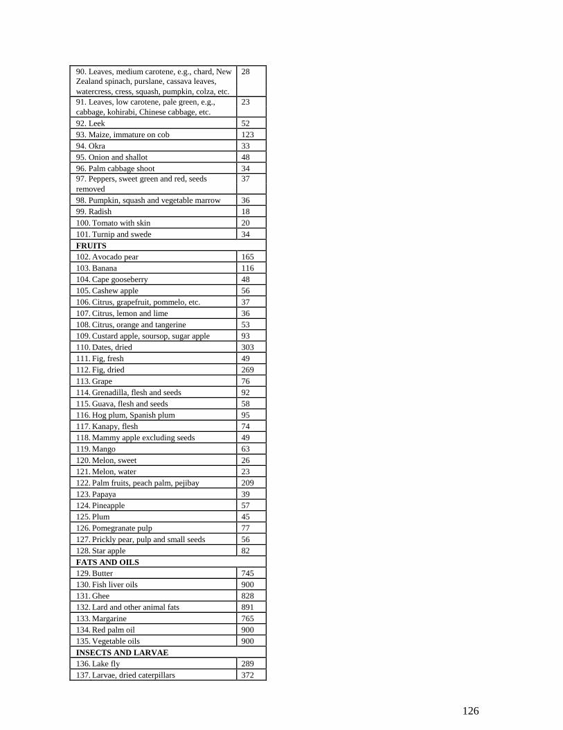
90. Leaves, medium carotene, e.g., chard, New 28 Zealand spinach, purslane, cassava leaves,

watercress, cress, squash, pumpkin, colza, etc.

91. Leaves, low carotene, pale green, e.g., 23 cabbage, kohirabi, Chinese cabbage, etc.

92. Leek 52 93. Maize, immature on cob 123 94. Okra 33 95. Onion and shallot 48 96. Palm cabbage shoot 34 97. Peppers, sweet green and red, seeds 37 removed

98. Pumpkin, squash and vegetable marrow 36 99. Radish 18 100. Tomato with skin 20 101. Turnip and swede 34 FRUITS

102. Avocado pear 165 103. Banana 116 104. Cape gooseberry 48 105. Cashew apple 56 106. Citrus, grapefruit, pommelo, etc. 37 107. Citrus, lemon and lime 36 108. Citrus, orange and tangerine 53 109. Custard apple, soursop, sugar apple 93 110. Dates, dried 303 111. Fig, fresh 49 112. Fig, dried 269 113. Grape 76 114. Grenadilla, flesh and seeds 92 115. Guava, flesh and seeds 58 116. Hog plum, Spanish plum 95 117. Kanapy, flesh 74 118. Mammy apple excluding seeds 49 119. Mango 63 120. Melon, sweet 26 121. Melon, water 23 122. Palm fruits, peach palm, pejibay 209 123. Papaya 39 124. Pineapple 57 125. Plum 45 126. Pomegranate pulp 77 127. Prickly pear, pulp and small seeds 56 128. Star apple 82 FATS AND OILS

129. Butter 745 130. Fish liver oils 900 131. Ghee 828 132. Lard and other animal fats 891 133. Margarine 765 134. Red palm oil 900 135. Vegetable oils 900 INSECTS AND LARVAE

136. Lake fly 289 137. Larvae, dried caterpillars 372

126

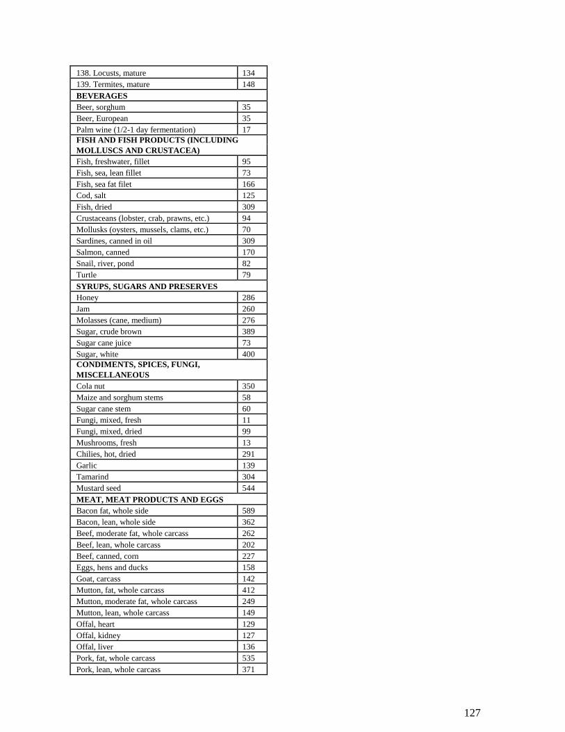
138. Locusts, mature 134 139. Termites, mature 148 BEVERAGES

Beer, sorghum 35 Beer, European 35 Palm wine (1/2-1 day fermentation) 17 FISH AND FISH PRODUCTS (INCLUDING MOLLUSCS AND CRUSTACEA)

Fish, freshwater, fillet 95 Fish, sea, lean fillet 73 Fish, sea fat filet 166 Cod, salt 125 Fish, dried 309 Crustaceans (lobster, crab, prawns, etc.) 94 Mollusks (oysters, mussels, clams, etc.) 70 Sardines, canned in oil 309 Salmon, canned 170 Snail, river, pond 82 Turtle 79 SYRUPS, SUGARS AND PRESERVES

Honey 286 Jam 260 Molasses (cane, medium) 276 Sugar, crude brown 389 Sugar cane juice 73 Sugar, white 400 CONDIMENTS, SPICES, FUNGI,

MISCELLANEOUS

Cola nut 350 Maize and sorghum stems 58 Sugar cane stem 60 Fungi, mixed, fresh 11 Fungi, mixed, dried 99 Mushrooms, fresh 13 Chilies, hot, dried 291 Garlic 139 Tamarind 304 Mustard seed 544 MEAT, MEAT PRODUCTS AND EGGS

Bacon fat, whole side 589 Bacon, lean, whole side 362 Beef, moderate fat, whole carcass 262 Beef, lean, whole carcass 202 Beef, canned, corn 227 Eggs, hens and ducks 158 Goat, carcass 142 Mutton, fat, whole carcass 412 Mutton, moderate fat, whole carcass 249 Mutton, lean, whole carcass 149 Offal, heart 129 Offal, kidney 127 Offal, liver 136 Pork, fat, whole carcass 535 Pork, lean, whole carcass 371

127

Pork, salt, fat 781 Poultry, chicken, duck, turkey, etc. 139 Rabbit 134 Veal, moderately fat 184 MILK AND MILK PRODUCTS

Cheese from whole cow’s milk, hard 384 Cheese from skimmed cow’s milk, soft 87 Milk, cow, whole 64 Milk, human 75 Milk, buffalo 102 Milk, goat 71 Milk, sheep 108 Milk, cow, skimmed 34 Milk, cow, whole, condensed 140 Milk, cow, whole, condensed, sweetened 317 Milk, cow, whole, powder (unmodified) 500 Milk, cow, skimmed, condensed, sweetened 276 Milk, cow, skimmed, powder 357

128

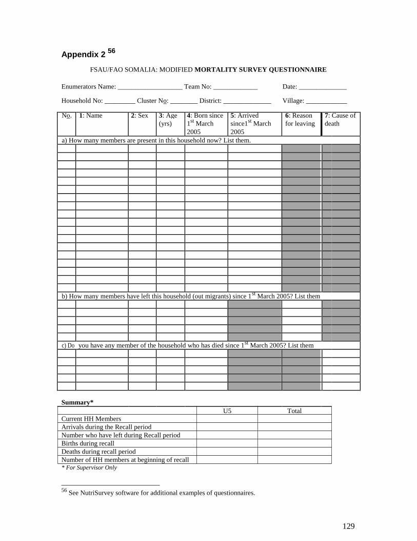
Appendix 2 56

FSAU/FAO SOMALIA: MODIFIED MORTALITY SURVEY QUESTIONNAIRE

Enumerators Name: ___________________ Team No: _____________ Date: ______________

Household No: _________ Cluster No: ________ District: ______________ Village: ____________

No. 1: Name 2: Sex 3: Age 4: Born since 5: Arrived 6: Reason 7: Cause of (yrs) 1

st March since1

st March for leaving death

2005 2005

a) How many members are present in this household now? List them.

b) How many members have left this household (out migrants) since 1st

March 2005? List them

c) Do you have any member of the household who has died since 1st

March 2005? List them

Summary* U5 Total

Current HH Members Arrivals during the Recall period Number who have left during Recall period Births during recall Deaths during recall period Number of HH members at beginning of recall * For Supervisor Only

56 See NutriSurvey software for additional examples of questionnaires.

129