Embed Size (px)
Citation preview

Measuring Productivity with Non-conventional Approach Comment by Harry X. Wu on papers by#1) Cecilia Kwok-ying Lam#5) Hideyuki KamiryoSession 6C

The Conventional Approach (Solow-Jorgenson) An input-output approach Substitute the income share of factors in
national accounts for the output elasticity of input factors to weight input (K, L, M) growth, then derive a “growth residual” that cannot be explained by the weighted input growth - TFP
This assumes (strongly) that factors are paid their marginal social products, then profit-maximising agencies operate in a distortion-free market system with perfect competition

… methodologically
Assume input homogeneity Impose CRS, (logically) assuming that the
sum of factor incomes is equal to national income or GDP.
Impose neutral technological progress restriction, assuming that the economy is operating on the frontier and hence no inefficient agency exists.

The question is…in reality
What if Inefficient firms exist operating off the PPF? Market imperfection? – firms with market
power Government intervention, hence price
distortion? Some sectors (e.g. the government sector)
are not subject to market principles?

Estimating Cross-country Technical Efficiency, Economic Performance and Institutions – A Stochastic Production Frontier Approach
The 2006 Ruggles Travel Grant Paper
By Cecilia Kwok-ying Lam
The University of Birmingham
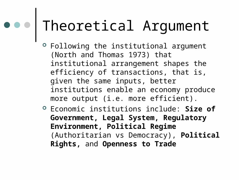
Theoretical Argument Following the institutional argument (North and
Thomas 1973) that institutional arrangement shapes the efficiency of transactions, that is, given the same inputs, better institutions enable an economy produce more output (i.e. more efficient).
Economic institutions include: Size of Government, Legal System, Regulatory Environment, Political Regime (Authoritarian vs Democracy), Political Rights, and Openness to Trade

Methodology
Productivity measurement is a crucial measure of cross-country growth performance. However, measuring cross-sectional technical efficiency with standard growth accounting cannot serve the theoretical framework. Therefore, the stochastic production frontier (SPF) approach that measures technical efficiency is adopted.
SPF (Fare, Grosskopf et al. 1994) decomposes productivity into changes in efficiency (catching up) and changes in technology (innovation). Each country is compared to a frontier. How much a country getting closer to the “world frontier”
measures the “catching up” effect How much the world frontier shifts indicates “technical
change” or “innovation” effect

Following Aigner, Lovell et al. (1977) and Meeusen and Broeck (1977), the stochastic production frontier function (thereafter abbreviated as SPF) can be extended as: )exp(; iiii uvxfy
Assume v is a stochastic error independently distributed of u. It accounts for the measurement such as the effects of weather, strikes, luck etc, on the value of the output variable together with the combined effects of unspecified input variables.
u is assumed to be a non-negative random variables associated with technical inefficiency of production and is independently distributed.
if u=0, then sum of 2-sided errors (u+v) = v, the error term is symmetric, and the data do not support a technical inefficiency story. However, if u > 0, then v – u is negatively skewed, and there is evidence of technical inefficiency in the data.

Specification
Stochastic Production Frontier
Technical Inefficiency Model
itittiii
iiiititiit
uvtimelatinsaseca
mideasteasiaafricaLKY
9876
54320 lnlnln
itit wopennesspoliticgovu 321

Data (1) – Production Function
Y: Real GDP (PPP adjusted) (Penn World Table)
K: Capital (from investment data) (Penn World Table)
L: Labour force (World Development Indicators)
Year: 1980-2000; Countries: 80 5-year average; 4 periods; 320 obs

Data (2) – The Role of the State (Gwartnet, Lawson et al 2002) GOV – government consumption / total
consumption TRS – Size of transfer and subsidies over
GDP COURT – index of impartial court PROPR – index of intellectual property rights CREDIT – credit market regulation index LABOR – labour market regulation index

Data (3) – Political Institution
POLITY IV database (2003)
REGIME – regime type, from authoritative to democratic
DURABLE – durability of the regime type
XCONST – operational (de facto) independence of chief executive
PR – political rights (Freedom House 2004)
Data (4) – International Trade (Gwartnet, Lawson et al 2002)
FOREIGN – free to own foreign currency bank account domestically and abroad
TRADEB – regulatory trade barriers, hidden import barriers and cost of importing
BLACK – black market exchange rate premium

Results (1a) – Production Function (lnY)
ind. var. coefficient (standard error)
constant 3.6979*** (0.1799)
lnK 0.6368*** (0.0133)
lnL 0.3427*** (0.0152)
time 0.0010 (0.0098)
africa 0.0640 (0.0436)
latin 0.0807** (0.0383)
easia 0.0047 (0.0519)
eca -0.0216 (0.0550)
sas -0.1127 (0.0593)
mideast 0.0360 (0.0507)

Results (1b) – Sources of TE (u)
ind. var. coefficient (standard error)
GOV 0.0231*** (0.0050)
TRS -0.0456*** (0.0124)
COURT -0.0411** (0.0199)
PROPR 0.2386*** (0.0489)
COURT * PROPR -0.0192*** (0.0062)
CREDIT -0.0261** (0.0121)
LABOR -0.0171 (0.0146)
DURAB -0.0068*** (0.0009)
XCONT 0.0492* (0.0299)
REGIME -0.0050 (0.0142)
PR 0.0517** (0.0243)
FOREIGN -0.0135 (0.0089)
TRADEB -0.0680** (0.0270)
BLACK -0.0099 (0.0092)
σ2 0.0756*** (0.0115)
γ 0.8260*** (0.0434)
log (likelihood) 106.9769
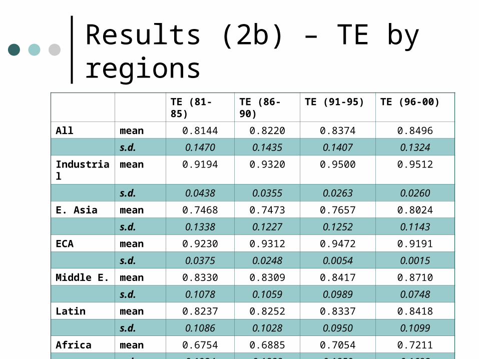
Results (2b) – TE by regions
TE (81-85) TE (86-90) TE (91-95) TE (96-00)
All mean 0.8144 0.8220 0.8374 0.8496
s.d. 0.1470 0.1435 0.1407 0.1324
Industrial mean 0.9194 0.9320 0.9500 0.9512
s.d. 0.0438 0.0355 0.0263 0.0260
E. Asia mean 0.7468 0.7473 0.7657 0.8024
s.d. 0.1338 0.1227 0.1252 0.1143
ECA mean 0.9230 0.9312 0.9472 0.9191
s.d. 0.0375 0.0248 0.0054 0.0015
Middle E. mean 0.8330 0.8309 0.8417 0.8710
s.d. 0.1078 0.1059 0.0989 0.0748
Latin mean 0.8237 0.8252 0.8337 0.8418
s.d. 0.1086 0.1028 0.0950 0.1099
Africa mean 0.6754 0.6885 0.7054 0.7211
s.d. 0.1924 0.1888 0.1850 0.1692

Results (3b)
East Asia and Pacific
Period Output Growth
(%)
Capital Growth
(%)
Labour Growth
(%)
TFP Growth
(%)
TE change
(%)
81-85 5.19 9.05 2.67 -1.49 ..
86-90 7.02 6.45 2.49 2.06 0.07
91-95 7.00 8.46 2.30 0.82 2.42
96-00 4.00 6.67 2.11 -0.97 4.69
81-00 5.80 7.66 2.39 0.11 7.18
Main conclusion
Economic performance as expressed in terms of technical efficiency (TE) is drastically different from that expressed in total factor productivity (TFP) growth.
All three institutional aspects are important in explaining technical efficiency (TE) across countries.
Domestic economic and political institutions account TE more than whether the country is openness to trade and capital flow. In other words, local governance matters more than whether an open economy strategy is adopted.

Questions
It is difficult to accept that the measure of inefficiency of other countries with the US as the frontier. Given different factor endowments across countries, a country could be operating on its own frontier but still below the US benchmark.
More explanation may be needed to discuss the results for the fast growing east Asia economies – least efficient after Africa?
More detailed discussion of data

Productivity Comparisons by Country: The Government Sector vs the Private Sector
By Hideyuki Kamiryo Hiroshima Shudo University

Problems with the conventional approach The conventional growth accounting
approach with aggregate production function assumes that the government sector (G) and the private sector (PRI) are subject to the same production function, which violates the competitive market assumption
Studies at industry level (Jorgenson type) mainly focus on the business sector

Problems with the conventional approach… Measuring capital and rents (the rate
of return) for G is impossible; e.g. the Canberra Group may use (2008) expected rate of return which is not additive with the private sector
However, the G sector has significant bearing on TFP measure, especially when the size of government is large and the budget deficit is large

The New Approach: Reformation of SNA based on National Disposable Income (NDI)
Y=W+=(WG+G)+(WPRI+PRI) where Y=YG+YPRI, =Y − W, G =YG − WG,
and PRI =YPRI − WPRI . Wages are those after being modified by consumption of NDI.
NDI: after taxes and depreciation. National accounts are modified by NDI, hence
they become consistent as a whole macro accounting system and satisfy the additivity requirement for sectors.
Now, we can shift to the measurement of TFP

Preliminary method for productivity comparison
Measuring capital and rents (the rate of return) simultaneously by sector
(1) 1-=c/(rho/r) determined by national taste: (rho/r)=1 for the government sector and (rho/r)≠1 for the private sector
(2) k=(/(1-))/(r/w). As a result, the capital-output ratio and the rate of return
(under marginal productivity) are derived.

The structure of productivity (ALP, TFP, and ACP)
In the transitional path (from DRS/IRS at the current situation to CRS at convergence), the bypass production function (using TFP as a residual in a narrow sense; see below) converges to the C-D production function
ALP, TFP, and ACP, in the transitional path: ALP and ACP that are partly qualitative. TFP that is purely qualitative.

TFP (in this study) is the product of the TFP as a residual (in a narrow sense) (TFPRESI) and the capital-output ratio with a power that controls the shift from DRS/IRS to CRS.
The product of TFP and the capital-output
ratio is 1.0 under convergence: 1.0=*B*^(1-) and 1.0=k^().
TFP differs from the current year’. BTFP=TFP/k and B=(1-)/.
The structure of productivity (ALP, TFP, and ACP)…

Figures:1-=c/(rho/r),(r/w) to 1-, and r(0) to 1-
(rho/r )(c ) of three Clubs 30 countries 1995-2004
y = -1.0216x2 + 2.5726x - 0.4771
R2 = 0.8771
0.5
0.6
0.7
0.8
0.9
1.0
1.1
1.2
0.40 0.50 0.60 0.70 0.80 0.90 1.00 1.10c
rho/
r
(rho/r )(c ) of Club s that includes 8 countries 1995-2004
y = -46.2x2 + 82.06x - 35.44
R2 = 0.4643
0.92
0.93
0.94
0.95
0.96
0.97
0.98
0.99
1.00
1.01
1.02
0.82 0.83 0.84 0.85 0.86 0.87 0.88 0.89 0.90
c=C/Y
rho/
r
r/w and 1-alpha : 30 countries in 1995-2004
0.00
0.01
0.02
0.03
0.04
0.05
0.06
0.07
0.78 0.80 0.82 0.84 0.86 0.88 0.90 0.92 0.94 0.96 0.98 1.00
1-alpha
The rate of return, r (0), and the capital-output ratio, (0):Total economy of 30 countries 1995-2004
0.00
0.05
0.10
0.15
0.20
0.25
0.30
0.35
0.40
0.45
0.50
0.0 0.5 1.0 1.5 2.0 2.5 3.0 3.5 4.0the capital-output ratio, (0)
r(0)

Tables: (1) The US, Russia, China, India, and Japan,(2) The US versus Japan
(0) The U S (8) Russia (6) China (2) India (6) Japan
G/*GRI/*PRI
G/*G
RI/*PRI
G/*GRI/*PRI
G/*G
RI/*PRI
G/*GRI/*PRI
1996 0.867 1.080 0.722 1.283 1.138 1.054 1.284 1.169 0.928 1.2291997 1.081 1.082 0.868 1.324 1.121 1.074 1.139 1.199 0.945 1.1801998 1.202 1.080 1.769 1.087 1.116 1.090 1.102 1.222 0.695 1.2901999 1.141 1.090 0.985 1.001 1.090 1.098 1.067 1.224 0.968 1.3282000 1.243 1.071 1.291 1.232 1.083 1.111 1.470 1.193 1.121 1.3042001 1.041 1.102 1.379 1.203 1.049 1.136 0.645 1.181 3.496 1.3622002 1.033 1.166 1.485 1.100 1.144 1.118 2.160 1.167 5.159 1.3592003 0.951 1.138 1.622 1.087 1.219 1.108 0.885 1.166 (8.341) 1.2692004 0.748 1.118 2.566 1.083 1.187 1.107 1.059 1.155 (0.868) 1.234
The US JapanG sector ALP=y G TFP G k G
G
1/ACPG=G ALP=y G TFP G k G
G
1/ACPG=G
1995 19.88 26.13 24.69 (0.085) 1.242 5.68 4808 12374 (0.062) 4.6161996 21.59 25.05 26.22 (0.045) 1.215 5.16 4566 12947 (0.053) 4.6961997 24.64 21.28 27.46 0.044 1.115 5.72 3803 13638 (0.029) 4.7291998 26.86 20.11 28.99 0.086 1.079 5.88 41563714 13890 (1.079) 9.8441999 30.14 18.55 29.99 0.143 0.995 4.97 82051 13940 (0.384) 6.6552000 33.71 17.58 31.33 0.189 0.929 5.06 62111 13878 (0.353) 6.4552001 31.42 21.85 31.98 0.105 1.018 4.43 321700 13282 (0.544) 7.2122002 25.79 36.81 31.44 (0.103) 1.219 6.75 4415684 12861 (0.843) 8.4612003 24.17 52.69 31.78 (0.225) 1.315 8.55 3695951 12593 (0.827) 8.3442004 25.69 54.57 32.81 (0.216) 1.277 12.12 4796512 12435 (0.856) 8.298

Tables: (2) The US versus Japan
The US JapanTaxes/Y (S-I )G /Y C G /Y S G /Y Y G /Y Taxes/Y (S-I )G /Y C G /Y S G /Y Y G /Y
1995 0.157 (0.022) 0.171 (0.013) 0.157 0.167 (0.056) 0.178 (0.010) 0.1671996 0.159 (0.016) 0.166 (0.007) 0.159 0.171 (0.057) 0.180 (0.009) 0.1711997 0.171 (0.000) 0.164 0.008 0.171 0.174 (0.046) 0.179 (0.005) 0.1741998 0.176 0.007 0.161 0.015 0.176 0.089 (0.138) 0.185 (0.096) 0.0891999 0.187 0.019 0.161 0.027 0.187 0.139 (0.093) 0.193 (0.053) 0.1392000 0.198 0.029 0.161 0.037 0.198 0.148 (0.081) 0.200 (0.052) 0.1482001 0.183 0.010 0.163 0.019 0.183 0.135 (0.080) 0.208 (0.073) 0.1352002 0.155 (0.024) 0.171 (0.016) 0.155 0.117 (0.099) 0.215 (0.098) 0.1172003 0.143 (0.040) 0.175 (0.032) 0.143 0.118 (0.092) 0.215 (0.097) 0.1182004 0.144 (0.038) 0.175 (0.031) 0.144 0.115 (0.091) 0.214 (0.099) 0.115
The US The G sector versus the total economy Japan The G sector versus the total economy
g A (FLOW)G g A (TFP)G g A (FLOW ) g A (TFP ) i=I/Y g A (FLOW)G g A (TFP)G g A (FLOW ) g A (TFP ) i=I/Y
1996 0.089 (0.041) 0.046 0.045 0.096 0.031 (0.050) 0.011 (0.007) 0.1261997 0.139 (0.151) 0.040 0.034 0.099 0.048 (0.167) 0.012 0.012 0.1211998 0.086 (0.055) 0.039 0.045 0.106 (0.492) 10928 (0.027) (0.006) 0.0991999 0.117 (0.077) 0.048 0.052 0.111 0.483 (0.998) (0.016) 0.020 0.0912000 0.110 (0.053) 0.034 0.061 0.114 0.023 (0.243) (0.000) 0.019 0.0882001 (0.071) 0.243 0.029 0.017 0.104 (0.171) 4.179 (0.014) (0.077) 0.0752002 (0.185) 0.685 0.013 (0.008) 0.092 (0.203) 12.726 (0.004) 0.003 0.0562003 (0.061) 0.432 0.034 0.033 0.092 (0.025) (0.163) (0.004) (0.093) 0.0522004 0.070 0.036 0.051 0.055 0.102 (0.018) 0.298 0.019 (0.048) 0.054

Some questions to discuss
How can we connect “operating surplus and wages/compensation in GDP” with “consumption and saving in NDI” after depreciation and tax redistribution?
It is not very clear about the concept of the duality between the TFP that represents whole qualities (i.e., TFP is not a residual but an essence of technology) and the capital and labor that represent whole quantities?
What distinguishes the “qualitative” in the current investment and the “qualitative” in the level of technology accumulated in the past?
Has the quality change of inputs been considered in line with the idea of “converting better to more” (Jorgenson)?