Version 1.0

1

Measuring Support to Energy — Version 1.0

by the OECD Secretariat1

May 2010

Background paper to the joint report by IEA, OPEC, OECD and World Bank on “Analysis of

the Scope of Energy Subsidies and Suggestions for the G-20 Initiative”

1 Contacts: Ronald Steenblik (ronald.steenblik@oecd.org), Jens Lundsgaard (jens.lundsgaard@oecd.org),

Stephen Matthews (Stephen.matthews@oecd.org) or Olga Melyukhina (Olga.Melyukhina@oecd.org).

Version 1.0

2

TABLE OF CONTENTS

ACRONYMS AND ABBREVIATIONS ........................................................................................................ 4

PART I MAIN CONCEPTS ......................................................................................................................... 5

CHAPTER 1. INTRODUCTION .................................................................................................................... 5

1.1. Objective ............................................................................................................................................... 5 1.2. Structure ................................................................................................................................................ 6

CHAPTER 2. OVERVIEW OF SUBSIDY DEFINITIONS AND INDICATORS ........................................ 7

2.1. Definitions of subsidy ........................................................................................................................... 7 2.2. Overview of support indicators: key terms, definitions and distinctions ............................................ 10 2.3. Basic principles of measuring support ................................................................................................ 10

CHAPTER 3. IDENTIFYING, DISTINGUISHING AND CLASSIFYING POLICIES ............................. 12

3.1. Identifying support policies ................................................................................................................ 12 3.2. Distinguishing among policies according to economic group ............................................................ 13 3.3. Classifying and labelling support policies .......................................................................................... 14

3.3.1 Policies that support producers individually (PSE) ....................................................................... 14 3.3.2 Policies that support consumers (CSE) ......................................................................................... 17 3.3.3 Policies that support producers or consumers collectively (GSSE) .............................................. 17

PART II. CALCULATING SUPPORT INDICATORS ............................................................................... 19

CHAPTER 4. ESTIMATING POLICY TRANSFERS: PRICE TRANSFERS ........................................... 19

4.1. Price transfers arising from policy measures ...................................................................................... 19 4.2. Selecting and adjusting prices ............................................................................................................. 19

Internationally traded commodities ........................................................................................................ 21 Non-traded commodities ........................................................................................................................ 23 4.1.1 Price transfers to producers ........................................................................................................... 24

4.2 Price transfers to or from consumers ................................................................................................... 24 4.2.1 Calculating price transfers to consumers based on the price gap method ..................................... 24 4.2.2 Alternative methods for calculating consumer subsidies .............................................................. 24

CHAPTER 5. ESTIMATING OTHER TRANSFERS .................................................................................. 27

5.1. Budgetary transfers ............................................................................................................................. 27 Government grants related to assets ....................................................................................................... 28 Adjustments ............................................................................................................................................ 29

5.2. Support based on revenue foregone .................................................................................................... 30 5.2.1. Tax expenditures .......................................................................................................................... 30 5.2.2. Preferential lending ...................................................................................................................... 33 5.2.3. Debt concessions .......................................................................................................................... 35 5.2.4. Administered input prices ............................................................................................................ 35

5.3 Allocation of support to support categories and recipient categories .................................................. 36

CHAPTER 6. CALCULATING INDICATORS OF SUPPORT .................................................................. 37

6.1. Support to producers .......................................................................................................................... 37 6.1.1. Producer Support Estimate (PSE) ................................................................................................ 37 6.1.2. Percentage PSE (%PSE) ............................................................................................................... 37 6.1.3. Producer Nominal Assistance Coefficient (Producer NAC) ........................................................ 37

Version 1.0

3

6.1.3. Producer Nominal Protection Coefficient (Producer NPC) ......................................................... 38 6.2. Support to consumers .......................................................................................................................... 39

6.2.1. Consumer Support Estimate (CSE) .............................................................................................. 39 6.2.2. Percentage CSE (%CSE) and Consumer Nominal Assistance Coefficient (Consumer NAC) .... 40 6.2.3. Consumer Nominal Protection Coefficient (Consumer NPC) ..................................................... 40

6.3. General Services Support .................................................................................................................... 41 6.3.1 General Services Support Estimate (GSSE) .................................................................................. 41 6.3.2 Percentage GSSE (%GSSE) .......................................................................................................... 41

6.4. Total Support ...................................................................................... Error! Bookmark not defined. 6.4.1 Total Support Estimate (TSE) ....................................................................................................... 41 6.4.1 Percentage TSE (%TSE) ............................................................................................................... 42

6.5. Calculating indicators of support for groups of countries or for the world ......................................... 42 6.5.1. Conversion into a common currency ............................................................................................ 42 6.5.1. Aggregation to regional or global totals ....................................................................................... 42

CHAPTER 7. DATA AND INFORMATION REQUIREMENTS FOR CALCULATING THE

INDICATORS ............................................................................................................................................... 43

7.1. Requirements for calculating price transfers ...................................................................................... 43 7.2 Requirements for calculating budgetary and other transfers ................................................................ 44

GLOSSARY .................................................................................................................................................. 45

REFERENCES .............................................................................................................................................. 46

Boxes

Common forms of tax expenditure ............................................................................................................ 30

Version 1.0

4

ACRONYMS AND ABBREVIATIONS

AC Code used for policies included in All Commodity Transfers

ACT All Commodity Transfers

AMS Aggregate Measurement of Support

CIF Cost, Insurance and Freight

CSE Consumer Support Estimate

ERA Effective Rate of Assistance

ERP Effective Rate of Protection

EU European Union

FAO Food and Agricultural Organisation of the United Nations

FOB Free on Board

G-20 Group of Twenty

GC Group Commodity

GCT Group Commodity Transfers

GDP Gross Domestic Product

GSSE General Services Support Estimate

GTAP Global Trade Analysis Project

IMF International Monetary Fund

LC Local Currency

LV Price Levies

MFN Most Favoured Nation

MPD Market Price Differential

MPS Market Price Support

NAC Nominal Assistance Coefficient

NGO Non-government organisation

NPC Nominal Protection Coefficient

NRA Nominal Rate of Assistance

NRP Nominal Rate of Protection

OECD Organisation for Economic Co-operation and Development

OTC Other Transfers from Consumers

OT Code used for policies included in Other Transfers to Producers

OTP Other Transfers to Producers

PSE Producer Support Estimate

SCT Single Commodity Transfers

T Metric Tonne

TCT Transfers to Consumers from Taxpayers

TPC Transfers to Producers from Consumers

TPT Transfers to Producers from Taxpayers

TRQ Tariff-Rate-Quota

TSE Total Support Estimate

US United States of America

VAT Value Added Tax

WTO World Trade Organisation

Version 1.0

5

PART I MAIN CONCEPTS

CHAPTER 1. INTRODUCTION

1. The interest of the G-20 Group in measuring subsidies to energy, and in particular to fossil fuels,

is strongly related to the environmental and domestic economic effects of those subsidies. In their

statement issued at the conclusion of their 24-25 September 2009 summit in Pittsburgh, Pennsylvania, the

G-20 Leaders noted that:

Enhancing our energy efficiency can play an important, positive role in promoting energy

security and fighting climate change. Inefficient fossil fuel subsidies encourage wasteful

consumption, distort markets, impede investment in clean energy sources and undermine efforts

to deal with climate change.

2. Quantifying support, and explaining how the various support elements interact, will be essential

for countries to track their progress in implementing the G-20 Leaders‘ commitment to ―rationalize and

phase out over the medium term inefficient fossil fuel subsidies that encourage wasteful consumption‖. A

comprehensive and consistent quantitative method for measuring the subsidies generated by different

policies is needed to evaluate the extent of policy reform achieved by countries, both over time and

through specific reform efforts. . Nothing speaks louder about intentions of government policy than how its

actions direct transfers among taxpayers, government bodies, producers and consumers. Support indicators

can establish a common base for policy dialogue by using a consistent and comparable method to evaluate

the nature and incidence of policies. In the realm of agricultural and fisheries policy, for example, the

development of internationally comparable indicators and wide country coverage has made them useful

tools for policy dialogue not only among country groups, but also in inter-governmental forums (most

notably the WTO, OECD, IEA,World Bank, IMF and FAO), industry and non-government organisations.

3. Finally, if organized and in a way that takes into account the needs of analysts, estimates of

support can be of enormous use to researchers. The data can serve as an input into modelling to assess the

effectiveness and efficiency of policies in delivering the outcomes for which they were designed and to

understand their effects on production, trade, income, the environment, and so forth. While the indicators

cannot by themselves quantify these impacts, the economic information upon which they are based serves

as an important building block for further analysis.

1.1. Objective

4. This background paper is intended to help begin a discussion on methods for identifying,

estimating and classifying support to the energy sector. The methods explored in this annex include some

that have been applied to other sectors, as well as those that have mainly seen application in the energy

sector.

Version 1.0

6

5. The paper outlines a comprehensive and consistent scheme for discussing support to any industry

organized by economic activity. This is the basis for the effective rate of assistance (ERA) indicator, as

well as for the family of indicators comprised of the producer support estimate (PSE), consumer support

estimate (CSE), and total support estimate (TSE). However, it recognizes that that data limitations may

require at times the use of subsets of these indicators, or alternative measurement techniques.

1.2. Structure

6. Part I provides an introduction to the basic concepts, as covered in Chapter 1. Chapter 2

introduces the main purpose and principles behind the calculations of the indicators. Chapter 3 explains the

criteria used to identify policies included in the calculation of the indicators, how to distinguish policy

transfers according to recipient, and, finally, how to classify policies.

7. Part II details the methodology for calculating the indicators. Chapter 4 explains the method used

to calculate transfers derived from policies that affect the market price received by producers of fuels and

electricity. Chapter 5 focuses on other transfers, including budgetary payments to producers and support

based on revenue foregone, notably tax and credit concessions. Chapters 6 and 7 show how these transfers

can be assembled to calculate indicators of support to producers and consumers respectively. Chapter 8

details the calculation of indicators that measure support that is provided to producers or consumers

collectively. Chapter 9 explains some of the issues that need to be considered when comparing support

indicators across countries or aggregating them to obtain multi-country totals. Chapter 10 concludes Part II

by outlining the data and information requirements for calculating the indicators of support.

Version 1.0

7

CHAPTER 2. OVERVIEW OF SUBSIDY DEFINITIONS AND INDICATORS

2.1. Definitions of subsidy

8. Dissimilarities in the concept, and therefore in the formal definition of a subsidy, arise largely

from differences in the way the term has come to be used in everyday speech and by professionals working

in separate economic and legal disciplines. Originally the term referred to funds granted to a king to

supplement or replace customs duties and other taxes collected by royal prerogative (Looney, 1999). It has

evolved since then to refer, in some definitions, to any unrequited financial assistance provided by a

government. Through time, also, one can observe the gradual accretion of various types of policy-related

transfers provided by governments and their agents, along with foregone revenues, to the more common

notion of a subsidy as a direct government payment (Figure 1).

Figure 1. Ever-widening definitions of “subsidy” or “support”

9. Most of these additional elements are now reflected in the current definition of a subsidy given in

the World Trade Organization (WTO) Agreement on Subsidies and Countervailing Measures (SCM

Agreement), which was signed at the end of the GATT-sponsored Uruguay Round of multilateral trade

negotiations. Although other inter-governmental bodies have developed their own, usually more succinct

definitions of a subsidy (or, in the case of the OECD, ―support‖), the WTO‘s definition currently serves as

the definition of a subsidy formally agreed by the majority of governments in the world.

10. Article 1 of the WTO‘s Agreement on Subsidies and Countervailing Measures defines a subsidy

as involving ―a financial contribution by a government or any public body within the territory of a Member

(referred to in this Agreement as ―government‖) … or price support in the sense of Article XVI of GATT

1994‖ that confers a benefit. Among the financial contributions covered by the definition are: (i) direct

transfers of funds (e.g. grants, loans, and equity infusion), potential direct transfers of funds or liabilities

(e.g. loan guarantees); (ii) the foregoing or non-collection of government revenue that would otherwise be

Version 1.0

8

due (e.g. fiscal incentives such as tax credits); and (iii) goods or services (other than general infrastructure)

provided by a government in kind, or goods purchased from companies in a way that confers a benefit to

that company (e.g., by paying a price that is higher than the market price). The definition also covers

situations in which ―a government makes payments to a funding mechanism, or entrusts or directs a private

body to carry out one or more of the type of functions illustrated in (i) to (iii) above which would normally

be vested in the government and the practice, in no real sense, differs from practices normally followed by

governments.‖

11. The WTO definition excludes two forms of support: that part of market price support (MPS) —

i.e., transfers between consumers and producers created as a result of one or more government

interventions — provided through tariff and non-tariff barriers; and subsidies for general infrastructure.

The first support element is not included in the ASCM definition for institutional reasons: tariffs and non-

tariff barriers are normally addressed at the WTO through different disciplinary mechanisms than

subsidies. The second exclusion is consistent with the focus of the WTO on the trade-distorting effect of

measures. Subsidies to general infrastructure are presumed to have little specific adverse effects on a

country‘s trade. (Of course, subsidies for infrastructure may well have an impact on the consumption of

energy, and therefore on emissions and other environmental effects.) The ASCM definition does, however,

include non-economically justifiable discriminatory pricing of services from government-owned

infrastructure as an input subsidy.

12. Only slightly more comprehensive than the WTO in its coverage is the notion of ―support‖

included in the OECD‘s subsidy indicator, the producer support estimate (PSE). The PSE incorporates all

the types of subsidies covered by the ASCM definition, plus market price support in all its forms. An

analogous indicator, the consumer support estimate (CSE) combines transfers affecting consumption.2

13. The measures that governments use to provide support vary enormously in terms of their

mechanisms and design, reflecting diverse domestic political and economic settings and, increasingly,

obligations in the international economic arena. Despite this diversity, policy measures applied in a country

within a given period of time can be brought together and expressed in one or several simple numbers —

called support indicators — which are comparable across time and between countries.

14. The notion that the ―subsidy equivalent‖ values of transfers generated by different policies can be

expressed in common units and combined into one aggregate indicator derives from the economic theory

of protection developed in the 1960s to evaluate the effects of tariffs (Corden, 1971). According to this

theory, the producer subsidy equivalent of a policy measure, whether an import tariff, export subsidy,

payment per unit of output or per unit of input, is the direct payment that a government would have to

make to producers (normalized to per unit of output) to generate the same impact on production as the

policy measure in question. What practitioners eventually realized, however, was that in fact what was

being measured were not true subsidy equivalents from the standpoint of the recipient, as the ultimate

incidence — what percentage of a given transfer ends up in the pocket of the intended recipient — of

different types of subsidies vary enormously. What was being measured, rather, was the gross cost to

government or consumers (in cases where prices are artificially elevated). Hence the change in the name to

producer support estimate.

2 The PSE-CSE framework is based on the framework preferred by many economists, the effective rate of

assistance (ERA), which is structured so as to produce an estimate of the net government assistance to an

industry or product that allows a comparison to be made between the value-added of the assisted sector to

the value-added that would be generated by the same, but unassisted sector (at the world or reference

price). The ERA takes into account not only support directed at an industry but the amount of support

indirectly received, or the tax paid, by the industry through subsidies or taxes applied to supplies of inputs

to the industry. A major limitation of the ERA is that it requires accurate data on value added, which can be

difficult to obtain.

Version 1.0

9

15. Besides differing in coverage, the way that individual subsidy elements are measured can also

differ among practitioners. Desai and Lee (1997), in a guidebook for the Asian Development Bank (ADB),

for example, make a distinction between ―financial subsidies‖ and ―economic subsidies‖. They define a

financial subsidy as ―the difference between cost (financial outlay) and project revenue, where cost

includes the actual incremental investment costs of the project plus the incremental operating and

maintenance costs, as well as a return on capital equivalent to the cost of borrowing or a target financial

return.‖ And they define an economic subsidy as ―the difference between input costs and output prices, but

with all input costs and output prices reckoned at their equivalent economic prices — i.e., reflecting their

true opportunity cost.‖ The distinction between a financial and an economic basis for subsidy measurement

can be illustrated more generally by the distinction between the cost to a government agency of loans it

makes at interest rates reflecting its own cost of borrowing. Its net financial cost may be zero, but the

economic cost (reflecting the difference between the market interest rate and the government interest rate)

may be positive. The authors note that both measurement approaches have their uses and recommend that

the ADB estimate both types of subsidies when evaluating projects in which they may invest.

16. The PSE and the various price-gap measurements of consumer subsidies that have been

generated by the IEA, World Bank and others generally start from an opportunity-cost perspective.

However, due to data limitations, it may not always be possible to know the opportunity cost of an input or

an output, so the usual practice is for the financial cost to the government to be used instead.

17. What constitutes an economic approach to defining a subsidy is itself the subject of much debate

among economists and those responsible for measuring subsidies. Donohue (2008: 6) writes:

Broadly speaking, subsidies can be seen in one of two ways: subsidies are given by governments

or subsidies are given by society. Almost all subsidy definitions available in the literature could

be seen as generally conforming to one of these perspectives on subsidies. … An economic

approach might be to define subsidies as ―transfers that distort the allocation of economic

resources‖ which would be a society-wide approach to defining subsidies. A more government-

oriented approach might be to define subsidies simply as financial payments from governments

to firms or consumers. … The distinction between subsidies derived from government action,

versus social subsidies, is profound, and includes many possibilities for refinement.

The etymology of the word ―subsidy‖ clearly points to a definition that has historically been closely

linked to the consequences of a government action. The notion of a ―social subsidy‖ — costs paid incurred

by society through not only taxes and higher prices, but also or instead through increases in costs not born

by economic agents generating those costs — is a more recent idea, usually associated with environmental

externalities. The inclusion of (negative) externalities in the definition of ―subsidy‖, however, changes the

term from one linked not only to a government action, but also government inaction. That is to say,

because externalities are intrinsic to virtually all economic activities, it would imply that somebody driving

a diesel truck (and emitting particulate pollution and CO2) in a country in a state of anarchy was being

―subsidized‖. Moreover, since there is a great interest in the environmental effects of subsidies, particularly

of fossil-fuel subsidies, including non-internalized externalities in the definition of a subsidy could lead to

double-counting. Yet it is a nonsense to speak of externalities as subsidies causing environmental harm, as

the environmental harm is already captured in the estimation of the externality.

18. Nonetheless, the basic argument, that when evaluating the impacts of government policies

externalities should be considered alongside subsidies, is sound. In order to avoid confusion, however, the

terms ―subsidy‖ and ―support‖ as used in this document refer to policy transfers resulting from government

action only.

Version 1.0

10

2.2. Overview of support indicators: key terms, definitions and distinctions

19. Energy policies may maintain domestic fuel prices below those at the country‘s border. They

may provide direct payments to energy producers, or grant them tax and credit concessions. Support is not

only comprised of budgetary payments that appear in government accounts, but also includes support of

market prices, as well as other concessions that do not necessarily imply actual budgetary expenditure,

such as tax concessions and investment insurance. The common element of all these policies is that they

generate transfers to, or among, corporations and individuals that produce or consume energy.

20. The concept of a transfer presumes both a source of the transfer and the existence of a recipient.

When analyzing support within a sector, consumers of commodities and taxpayers typically represent the

two most important sources of transfers — i.e. the economic groups bearing the cost of sectoral support.

However, in the case of energy, producers themselves may be a source of support, at least in the short or

medium term. This occurs in situations in which a government restricts exports (thus denying producers

opportunities to maximize their revenues), or when it caps domestic prices. However, often the producers

involved are state-owned enterprises, which means that, ultimately, it is the government that bears any

losses.

21. Critical to understanding the measurement of support based on transfers is the distinction

between the notions of ―the provision of support‖ and the ―impact of support‖ (i.e., the impacts of policy

transfers). Support estimates measure gross policy transfers only, i.e., the provision of support. They

measure, in other words, the level of effort made by governments, as implied by their sectoral policies. The

indicators discussed here do not account for the deadweight or other welfare losses associated with that

effort within the economic system. Such information can only be derived through general equilibrium and

partial equilibrium models.

22. The other important distinction is between initial incidence and final incidence. Support

measurements are concerned with the initial (statutory, or formal) incidence of a transfer — to whom the

transfer initially flows. However, as with taxes, a proportion of most transfers will leak to other economic

agents. For example, only a portion of a policy that provides USD 100 million for an increase in the

production of fuel ethanol will end up as extra producer net income, because that extra production will

require the purchase of feedstock and other inputs, the prices of which may rise as a result of the induced

demand. The actual impact of policies on its recipients will depend on, among other things, the basis upon

which support is provided (e.g. per tonne of output, per unit of input, per producer or consumer, etc.), the

level of support, and the responsiveness of producers and consumers to changes in the level of support.

23. The support measures themselves, therefore, are not intended to, nor do they in fact, measure the

impact of policy efforts on production, incomes, trade or the environment. This limitation is crucial for

understanding the proper use and interpretation of support estimates. Chapter 11 contains a detailed

discussion of how the indicators should be used and interpreted, and concludes with examples of mistakes

in interpretation that should be avoided.

2.3. Basic principles of measuring support

24. A number of principles, or general rules, are needed to guide the measurement of support. Those

listed below are drawn from the only codification of principles that has been produced to date, as

documented in the OECD‘s PSE Manual (OECD, 2009). Principles 1 to 3 determine the scope of policy

measures to be considered in estimating support and provide criteria for identifying which policies to focus

on within a complex mix of government actions. Principles 4 and 6 help to define the method for

measuring support and are important for interpreting the indicators:

Version 1.0

11

1. Principle 1: The generation of transfers to producers or consumers is a key criterion for the

consideration of a policy in the measurement of support. Policy measures generate explicit or

implicit transfers to supported individuals or groups. A sufficient criterion for inclusion of a

policy measure in the estimation of support is that producers or consumers, individually or

collectively, are the only, or the principal, intended recipients of economic transfers generated by

the measure.

2. Principle 2: In accounting for transfers, no consideration should be given to the nature, objectives

or economic impacts of a policy measure. This principle complements Principle 1, in that the

stated objectives, or perceived economic impacts of a policy measure, are not used as alternative

or additional criteria to determine the inclusion or exclusion of a policy measure in the estimation

of support.

3. Principle 3: General policy measures available throughout the entire economy — such as general

investment tax credits — are not considered in the estimation of support, even if such measures

create policy transfers to or from the sector under consideration. Thus, a situation of zero support

to the energy sector would occur when there are only general economy-wide policies in place

with no policies specifically altering the economic conditions for energy production.

4. Principle 4: Policy transfers can be defined in gross or net terms, i.e. as revenue (gross receipts)

or income (revenue less costs) generated by a policy measure. The general practice is to measure

transfers generated by policies in gross terms. The phrase gross transfers in the definitions

emphasises that no adjustment is made in the indicators for costs incurred by producers in order

to receive the support (e.g. costs to meet compliance conditions attached to certain payments), or

extra taxes generated as a result of the activity.

5. Principle 5: Policy transfers to individual producers are measured at the point that the product

leaves the property of the production stage under investigation. If the objective is to measure

support only to primary producers of energy, that would correspond to the mine or well-head.

Consequently, the word ―consumer‖ in the definitions and methodology, unless specified

otherwise, is to be understood as a first-stage buyer of a fuel or electricity. However, it is

important to underscore that most of the consumer subsidies to energy published to date have

been measured at the level of the final, not the first, consumer.

6. Principle 6: Policy measures supporting individual producers are classified according to

implementation criteria, such as: (i) the basis upon which support is provided (a unit of output or

of input, etc.); (ii) whether support is based on current or non-current production or consumption

parameters; and (iii) other criteria. These policy characteristics affect producer behaviour, and

distinguishing policies according to implementation criteria enables further analysis of policy

impacts on production, trade, income, the environment, etc.

25. These are the general principles applied in estimating the indicators of support. Along with the

more practical underpinnings of the methodology, they are developed further in the following chapters.

Version 1.0

12

CHAPTER 3. IDENTIFYING, DISTINGUISHING AND CLASSIFYING POLICIES

26. Before calculating the support indicators for any particular sector or country, it is important to

understand fully the range of policy measures used by governments to support economic activities and the

forms in which they are implemented.

27. The first section of this chapter defines the generic policy measures included in the measurement

of support. The following section differentiates the policies according to which of the three economic

groups the transfer is made. The remaining sections detail the various categories and labels that can be

attached to policy measures.

3.1. Identifying support policies

28. The range of policy measures included in the estimation of government support are determined

by the definitions and principles outlined in Chapter 2. In all cases, which government body is responsible

for the policy measure giving rise to a transfer should have no impact on the decision of whether to include

it or not. Policy measures supporting energy, for example, may fall under the responsibility of many

different government ministries, and not just the ministry formally responsible for energy policy, and at

different levels of government (central, provincial, prefectural or state). Alternatively, support arising from

policies implemented by a ministry responsible for a sector, but unrelated to the activities of the sector

being studied (e.g. agriculture or national defence), are normally excluded from the sectoral subsidy

account.

29. Support provided to producers by governments may be delivered through a wide range of

mechanisms: increasing the output price (Market Price Support); providing cash directly (a cheque from

the government); reducing the riskiness of investing in fixed capital (e.g., loan guarantee; investment

insurance); foregoing a payment that would otherwise be due to the government (e.g., a tax concession) or

reimbursing a tax or charge (e.g., as for fuel taxes in some countries); reducing the price of an input (e.g.,

electricity for mining) or of a value-adding factor (e.g., a wage subsidy); providing a service in kind (e.g.,

police protection of a pipeline) for free or at a price less than the producer would pay on the open market;

investing in knowledge-creating activities (e.g., research and development; education and training of

specialists).

30. Within the category of producer support, it may be useful to distinguish those forms of support

that create transfers directly to individual producers from those that benefit producers as a whole. In the

measurement of support to agriculture, for example, the OECD distinguishes policies that support

producers individually (as measured by the PSE) or consumers individually (as measured by the CSE)

from other policies that support producers or consumers collectively or indirectly (as measured by the

GSSE). In the OECD‘s GSSE for agriculture, for example, the latter indicator encompasses two types of

support measures:

government expenditures associated with policy measures that are included in the PSE, but which

are not received directly by farmers — for example, the cost to the government of storing and

disposing of price-supported commodities by the government or an appointed agency; and

Version 1.0

13

services that benefit primary agriculture but whose initial incidence is not at the level of

individual farmers — for example, agricultural education, research, marketing and promotion of

agricultural goods, general infrastructural investment relating to drainage, and irrigation, and

inspection services beyond the farm gate.

With respect to energy, analogous policies would be expenditures by governments on maintaining

stockpiles of petroleum or coal, and expenditure on energy-related education, research, marketing and

promotion, investment in general infrastructure relating to the transport of energy (but not predominantly

energy), such as roads and railroads; and services related to the verification of the quality standards of

transport fuels.

31. Regarding support benefitting consumers, policy measures that provide positive transfers to first

consumers of energy include direct payments to final consumers for the purchase of fuels or electricity, and

the value of transfers to consumers created through government interventions that artificially depress the

domestic price compared with a reference price. In countries wherein the market price for energy is kept

higher than the international reference price, it is not unheard of for governments also to provide payments

to heavy industries (notably aluminium, cement, iron and steel plants) to offset those higher prices.

3.2. Distinguishing among policies according to economic group

32. Identifying the full range of policies supporting a sector is largely a process of distinguishing

between policy measures on the basis of which economic group receives the transfer. Three economic

groups are identified, according to whether the policy measure provides transfers to producers individually

(PSE), to consumers individually (CSE), or to one or the other collectively as general services (GSSE).

Appropriately distinguishing between policies is important for correctly calculating the indicators that

measure the level and composition of support. This process can be aided by the following sequence of

questions.

33. Question 1: Does the policy create a transfer to the sector collectively through general services?

34. To answer in the affirmative, such transfers should not depend on the actions of individual

producers or consumers, be received by individual producers or consumers, and not affect directly

producer receipts or consumption expenditure. In answering this question, it may be useful to bear in mind

the categories for classifying policies within the GSSE (section 3.3.3). If the answer is yes, consider the

policy under the GSSE. If no, proceed to the next question.

35. Question 2: Does the policy measure create a transfer to producers individually based on goods

or services produced, on inputs used, or on the fact of being a productive enterprise?

36. For a policy measure to be included in the PSE, it is necessary that an individual producer takes

actions to produce goods or services, to use factors of production, or to be defined as an eligible producing

enterprise, in order to receive the transfer. If yes, consider it under the PSE.

37. Question 3: Does the policy create a transfer to or from consumers of the good or service?

38. In the case of the CSE, it is necessary for individual consumers to take actions to consume a good

or service in order to receive (or provide) a transfer. Examples of policies grouped in the CSE include

consumption subsidies in cash or in kind to support consumption levels, and transfers to processors (first

consumers) to compensate them for higher domestic prices. Note also that some policies that are grouped

in the PSE also appear in the CSE (but with an opposite sign). These relate to the policies that create output

price-based transfers. For example, a border tariff creates a price gap between domestic and world prices,

Version 1.0

14

resulting in consumers paying a higher price for that product. This policy measure results in transfers from

consumers to producers and from consumers to government revenue (sections 4.2 and 4.3 explain this in

greater detail). If yes, consider it under the CSE.

39. The TSE represents the sum of all three components, adjusted for double-counting given that the

transfers associated with market-price-support policies appear in both the PSE and the CSE calculations.

3.3. Classifying and labelling support policies

40. The impact of policy measures on variables such as production, consumption, trade, income,

employment and the environment depend on, among other factors, the way policy measures are

implemented. Therefore, to be helpful for policy analysis, policy measures to be included in the PSE are

classified according to implementation criteria. For a given policy measure, the implementation criteria are

defined as the conditions under which the associated transfers are provided to producers, or the conditions

of eligibility for the payment. However, these conditions are often multiple. Thus, the criteria used to

classify payments to producers are defined in a way that facilitates: the analysis of policies in the light of

the ―operational criteria‖. These should include both the transfer mechanism and the statutory incidence of

the policy measures (i.e., the transfer basis for each policy). Additional ―labels‖ may be added

distinguishing whether the basis is current or non-current, and whether production or consumption is

required or not. It is also often useful to distinguish whether constraints are placed on output levels or input

use, whether the payment rate is variable or fixed, and whether the policy transfer is specific or not as to

the commodities covered or excluded.

41. The key underlying principle is that policy measures should be classified according to the way

they are implemented. Policy measures with an environmental focus illustrate the role of implementation

criteria in the classification of support policies. Possible payments with an environmental objective include

cost-sharing for the installation of pollution-control equipment, or alternatively could be provided per unit

of emissions (e.g., to motivate an above-standard level of environmental performance). Although in both

cases the payments may have the same environmental objective, the way that they are implemented differs,

and the incentives provided to producers in terms of resource use and production decisions may differ.

Accordingly, the two cases should not be considered within the same support category.

3.3.1 Policies that support producers individually (PSE)

42. The categories and sub-categories listed in Box 1 have been constructed to identify the imple-

mentation criteria that are considered to be the most significant from an economic perspective. They

identify:

the transfer basis for support: output (category A), input (category B), receipts or incomes

(categories C, D and E), and non-commodity criteria (category F);

whether the support is based on a current (categories A, B, C, F) or non-current (historical or

fixed) basis (categories D and E);

whether production is required (categories C and D) or not (category E).

Version 1.0

15

Box 1. Terms and definitions of the PSE categories and sub-categories

A. Support based on commodity output:

A.1. Market price support (MPS) — transfers from consumers and taxpayers to producers arising from policy

measures that create a gap between domestic market prices and border prices of a specific good or service.

A.2. Payments based on output — transfers from taxpayers to producers from policy measures based on current output of a specific good or service.

B. Payments based on input use: transfers from taxpayers to producers arising from policy measures based on the use of specific inputs:

B.1. Variable inputs — transfers reducing the cost to a producer of a specific variable input or a mix of variable inputs, such as energy, water or chemicals.

B.2. Fixed capital formation — transfers reducing the investment cost of buildings, equipment.

B.3. Services — transfers reducing the cost of services (e.g., business services, training services) provided to individual producers.

B.4. Labour — transfers reducing the cost of employed labour, such as through wage subsidies or reductions in social charges.

B.5. Land — transfers reducing the cost of purchased or rented land.

C. Transfers from taxpayers to producers arising from policy measures based on current receipts or income, with current production of one or more goods or services required.

D. Transfers from taxpayers to producers arising from policy measures based on non-current (i.e. historical or fixed) receipts or income, with current production of one or more goods or services required.

E. Transfers from taxpayers to producers arising from policy measures based on non-current (i.e. historical or fixed) receipts or income, but production of a good or service is not required.

F. Payments based on non-commodity criteria: transfers from taxpayers to producers arising from policy measures based on:

F.1. Long-term resource retirement — transfers for the long-term retirement of factors of production from commodity production. The payments in this subcategory are distinguished from those requiring short-term resource retirement that are based on production criteria.

F.2. A specific non-commodity output — transfers for the use of resources to produce specific non-commodity

outputs of goods or services that are not required by regulations.

F.3. Other non-commodity criteria — transfers provided equally to all producers, such as a flat-rate or lump-sum payment.

G. Miscellaneous payments: transfers from taxpayers to producers for which there is insufficient information to allocate them to the appropriate categories.

—————————

1. The abbreviations represent: A – Area; R – Receipts; and I - Income

Version 1.0

16

43. In addition to classification into a category, each policy measure can be assigned several ―labels‖

that provide additional details on policy implementation (Box 2). The six labels contain information on the

constraints placed by policies on output and payment levels or input use, further specify the basis of

transfer, its commodity specificity and variability of payment rates. The alternatives offered by each label

are exhaustive, so that only one of the available options can be attributed to a payment.

Box 2. Common PSE labels

With or without current commodity production limits or limits to payments (w/ L or w/o L): defines whether or

not there is a specific limitation on current production associated with a policy providing transfers to producers. Applied in categories A – F.

With variable or fixed payment rates (w/ V or w/ F rates): a payment is defined as subject to a variable rate where

the formula determining the level of payment is triggered by a change in price, net revenue or income or a change in production cost. Applied in categories A – E.

With or without input constraints (w/ C or w/o C): defines whether or not there are specific requirements concerning

production practices related to the programme in terms of the reduction, replacement, or withdrawal in the use of inputs, or if restrictions are imposed on production practices allowed. Applied in categories A – F.

Payments conditional on compliance with basic requirements that are mandatory (with mandatory);

Payments requiring specific practices going beyond basic requirements and voluntary (with voluntary).

Based on receipts or income (R or I): Applied in categories C – E.

Based on a single product, a group of products or all products (SC, GC, AC): defines whether the payment is

granted for production of a single product, a group of products or all products. Applied in categories A – D.

44. Distinction between the terms ―PSE category‖ and ―PSE label‖ is a matter of presentation

convention. Labels only represent additional dimensions in which the PSE can be broken down and, like

the PSE categories, are defined in terms of implementation criteria rather than policy objectives. Labels

can be used as an alternative presentation of policy implementation; they also could theoretically be

presented as PSE sub-categories or sub-sub-categories. However, not all labels are applicable to all PSE

categories (A to F). For example, a label distinguishing payments based on area, receipts or income is by

definition redundant for policies in categories A (Support based on commodity output) and B (Payments

based on input use). Other labels could be introduced and presented as sub-categories if policy

developments warrant the change. In designing the structure of a PSE database, the choice between treating

a particular implementation criterion as a sub-category or a label is one of relative importance and

pragmatism, rather than a conceptual difference between these two options.

45. The label ―with or without current commodity production limits or limits to payments‖ relates,

for example, to a production quota associated with policy measures in category A. The label also applies to

policy measures that restrict the payment as such, either by explicitly setting a maximum amount of

payment, or by limiting the number of production units that may receive payment. For example, a

programme that provides a payment only on the first 60 million litres produced in a given year is labelled

as having a payment limit since payments cease beyond that output limit.

46. The label ―with or without input constraints‖ serves to distinguish all PSE transfers (except those

in category A.1) that can be provided under the condition that producers respect certain production

practices considered as environmentally friendly, or which address other societal concerns. A further

Version 1.0

17

distinction could be made between mandatory and voluntary input constraints. The former would include

requirements that relate to a generally applicable regulations, while the latter would go beyond general

regulations and are adopted by producers voluntarily.

3.3.2 Policies that support consumers (CSE)

47. The CSE includes price transfers to or from consumers. The normal case, especially in countries

that are net exporters of fossil fuels, is that transfers are made to consumers through administered pricing.

These transfers may exist alongside other subsidies in cash or in kind (including vouchers) linked to the

consumption of a particular energy product. As with production subsidies, limits may apply that restrict the

amount of subsidies that an individual or household may receive. This suggests that the labels With

variable or fixed payment rates (w/ V or w/ F) and Based on receipts or income (R or I) may apply.

48. When consumers pay more than the reference price for a fuel, such as because of an import tariff,

market transfers can be considered the inverse of transfers associated with market price support for the

production of commodities that are consumed domestically; these are called price transfers from

consumers. These transfers are the same as those included in the PSE under category A.1 Market Price

Support, but they are given an opposite sign in the CSE and adjusted to apply to quantities consumed (as

opposed to quantities produced in the PSE).

49. Sometimes, when domestic prices are above international prices, budgetary transfers may be

provided to first consumers of energy products where these are provided specifically to offset the higher

prices resulting from market price support. An example would be payments made to industrial consumers

of coal who pay the guaranteed minimum price to producers. Another example might be a price premium

for locally produced coal.

3.3.3 Policies that support producers or consumers collectively (GSSE)

50. Transfers classified under the GSSE relate primarily to payments to eligible private or public

services provided to producers or consumers generally. Unlike the PSE and CSE, GSSE transfers do not

directly affect producer revenue or expenditure by consumers, although they may affect production or

consumption of energy products in the longer term.

51. While implementation criteria are used to distinguish whether the transfer is allocated to the

GSSE or another category, the definition of the categories in the GSSE and the allocation of policy

measures to these categories largely depends on the nature of the service. Common GSSE categories are

listed below.

52. Research and development. This category includes payments to institutions for research related to

energy-production or transformation technologies and production methods. In most cases, these payments

include the financing of public research institutions (mostly through the budget of the ministry of energy),

as well as grants financed by public funding provided to private research institutions and universities.

53. Inspection services. This category includes payments to finance institutions for the control of fuel

quality and safety for consumers. In most cases, these services are financed by public (governmental)

organisations, and hence the budgets of these organisations are included in the GSSE. Should these

services be provided by private institutions, the GSSE should account only for the amount of public

finance granted to these institutions.

54. Infrastructure. This category includes public expenditure financing the development of

infrastructure that is not for the exclusive use of domestic producers. Special care should be given to

distinguish support between specific and non-specific infrastructure. For example, government support for

Version 1.0

18

the construction of dedicated petroleum or natural-gas pipelines should be included in the PSE, as direct

investment assistance.

55. Marketing and promotion. This category includes forms of government assistance to increase

sales of primary energy commodities, such as exhibitions, fairs, promotional campaigns, advertising, and

publications.

Version 1.0

19

PART II. CALCULATING SUPPORT INDICATORS

CHAPTER 4. ESTIMATING POLICY TRANSFERS: PRICE TRANSFERS

4.1. Price transfers arising from policy measures

56. Numerous government policy measures may affect the domestic market price of a good or

service, including measures imposed at the border, such as tariffs and export subsidisation, and quotas on

imports or exports. In the case of domestic market interventions, such as direct price administration and

publicly financed stockholding, they can also involve transfers to or from the government budget, which

have implications for taxpayers. Indeed, when consumer prices are subsidized, the gap normally has to be

made up by the government in one form or another.

57. All these policy interventions alter the domestic market price of a product compared with its

border price. This policy-induced price difference can be denoted as a market price differential (MPD):

MPD = DP - BP [4.1]

where: MPD is the market price differential, DP is the domestic market price, and BP is the border

(or reference) price.

58. The MPD is negative when the net effect of policies is to induce a lower domestic market price,

thereby encouraging consumption but discouraging production. It is positive when the policy induces a

higher domestic market price, thereby supporting production and, in the absence of other market

interventions, discouraging consumption. In the former case, policies place a tax on producers, and price

transfers to producers are designated with a negative sign. For a diagrammatical exposition of these effects,

see the PSE Manual (OECD, 2009).

59. Price transfers are the affected produced or consumed volume multiplied by the MPD, adjusted

as necessary for quality differences and transport margins (see below). In the OECD‘s terminology, price

transfers to producers are called market price support (MPS) and price transfers to consumers are called

market transfers (MT). The same terminology is used here.

4.2. Selecting and adjusting prices

60. The common approach to calculating an MPD for a commodity is to measure the difference

between a domestic market price (when there are policies that are known to distort domestic prices) and a

border price that represents the opportunity price (cost) for domestic market participants. The practice of

using reference prices based on international prices for traded goods derives from arguments of

opportunity cost. For an importing country, the true cost of a product is its import price. For an exporting

country, the true value of production at the margin is what its producers could obtain on the international

market. Even if the country can produce at a cost that is lower than the international price, according to this

logic, domestic production should be valued at the international price rather than at domestic supply costs.

Version 1.0

20

Box 3. Using a "neutral" baseline counterfactual

Subsidies must be measured against some baseline, some counterfactual situation. Neil Bruce, in a conceptual study that he wrote for the OECD (Bruce, 1990), advised that subsidies should ―be measured with respect to a counterfactual environment in which they do not exist, rather than as the deviation of the subsidy from its optimal value.‖ In fact, many renderings of what that ―counterfactual environment in which subsidies do not exist‖ might look like can be constructed.

When economists take numbers for budgetary grants and loans straight out of budget documents, and arrange them in subsidy accounts, the baseline they are implicitly using to define the subsidy is a very similar world but for one difference: the particular programme providing the subsidy does not exist. Yet the net value of such subsidies to the recipients will be to some extent offset by the increased taxes required to finance them. Adjusting subsidies to account for this effect would be impractical, and the results within the margin of error for the gross (unadjusted) subsidy. But, the theoretical point is worth bearing in mind when analysing the effects of large-scale changes in a country’s pattern of taxing and spending.

Things become more complicated when one applies a price-gap method to measure transfers generated by border protection (i.e. market-price support), or the value to users of under-priced goods or services provided by governments. That is because one of the variables, the reference price, would likely adjust to a new equilibrium in the absence of the policy that gives rise to the price gap being measured. If the government of a country that was a large producer of wheat, for example, were suddenly to announce that henceforth all border protection and export subsidies would disappear, that countries’ exports would drop in the short term and the reference price (usually the price at the border) would presumably rise.

1 The ―true‖ value of the subsidy, to critics of the simple price-gap method to measuring

market-price support, should thus be measured against the new equilibrium price, not the reference price prevailing while the price-support policy is in place. A similar argument is often used by beneficiaries of government programs to justify ―offsetting‖ subsidies or tariffs when overseas competitors are blamed for distorting prices in world markets.

This line of reasoning holds considerable appeal, and it cannot be faulted for being ―wrong‖ in any economic sense. But, from a practical standpoint, it raises numerous problems. First, if it is to be followed for the calculation of market price support, then to be consistent it must also be followed in the calculation of direct payments to producers that are tied to a predetermined target price — what in agricultural policy are referred to as ―deficiency payments‖. That is to say, in that parallel universe in which no deficiency payments are given, production of the affected commodity would have been less, its price higher, and the required deficiency payment would have been smaller. Why stop there? Should we not also take into account the simultaneous effects of all the other subsidies that influence production and consumption levels?

Extending this logic to its inevitable end, one could make an argument for defining the counterfactual for subsidy measurement to be a world in which all subsidies, everywhere, are removed. Measuring subsidies against such a stan-dard could only be done with the help of a computable general equilibrium (CGE) model, and a very detailed one at that. As Bruce (1990) wrote, ―Determining the hypothetical output and input prices in the economy inthe absence of a government sector constitutes a major computational general equilibrium exercise, and even if this were done, the results would be subject to so much uncertainty that they would be of little interest.‖ Granted, CGE models have ad-vanced since 1990, but redefining subsidies as welfare effects, without going through the intermediate step of docu-menting the actual transfers, would sever any link they once had with observable data (such as expenditures published in budget documents) and render them irrelevant for monitoring budgetary impacts and other transfer-related purposes.

1. This outcome would be even more likely were all producing countries to reform their policies altogether and at once.

Source : Steenblik (2003)

61. While the method for estimating a market price differential is, in principle, straightforward,

differences of opinion exist among analysts as to what reference price to use. Countries with large

endowments of energy resources, in particular, point to the fact that international prices may not represent

true opportunity costs, as a large shift in sales from a (previously subsidized) domestic market to the

international market would likely depress international prices. Moreover, international prices may be

Version 1.0

21

distorted by a variety of factors and can experience a high degree of volatility from one year to the next.

Analysts need to be aware of these limitations when using and interpreting the resulting estimates (Box 3).

62. Although, conceptually, the measurement of price transfers is straightforward, numerous

practical issues arise. Generically, these include (Plunkett et al., 1992):

Ensuring that the products being compared are as alike as possible, or that their prices can be

adjusted to account for quality differences.

When the price comparison involves a weighted average of several price series for a particular

product, ensuring that the product(s) chosen for establishing a reference price are representative

of the locally produced or consumed product.

Ensuring that the prices being compared are normalized to the same location, or can be adjusted

to take account differences in location, value-added level, and that they reflect the same ancillary

services or conditions of sale.

63. For traded goods, where there are no import or export restrictions, the favoured choice of

reference price is usually an international price at the border, adjusted for transport and internal distribution

costs. For goods that are not traded, the reference price is typically the domestic cost of supply. In the case

of energy, the main products that are traded internationally are anthracite, bituminous (hard) coal, crude

oil, petroleum products, and liquid biofuels, namely ethanol, biodiesel (and possibly, in the future,

synthetic paraffinic kerosene or ―bio-jet‖ fuel). Some cross-border trade in electricity and natural gas

occurs, mainly in Europe and North America, but a large number of national markets for these energy

carriers are, essentially, isolated. Similarly, though small volumes of peat and lignite briquettes are traded,

the bulk of peat and lignite consumed in the world is produced and consumed locally.

Internationally traded commodities

Selecting a domestic price

64. When making price comparisons for exported or import-competing products, the standard

practice in agriculture has been to measure the domestic price of a product at the point that it leaves the

producers‘ property. In the case of energy products, the corresponding ―factory-gate prices‖ would be

located as follow:

Bituminous coal and anthracite: at the mine-mouth

Crude petroleum: at the well-head

Petroleum products: the refinery gate (the ex-refinery price)

Where producer prices have not been available, analysts have made comparisons on the basis of

average wholesale or consumer prices.

65. However, in the field of energy, the domestic prices used for most MPD comparisons of traded

products have been either the price between producers and major industrial or power-plant consumers (in

the case of coal), which may be a ―factory-gate‖ or a delivered price, or a final consumer price.

Version 1.0

22

Selecting a border price

66. A number of border prices and alternative methods for estimating them may be used to calculate

MPDs. The choice of a border price for a given commodity in any country is determined by factors such as

market structures, specifically the net trade position of the commodity concerned, and data availability.

The net trade situation is defined by comparing total domestic consumption and production of the

commodity. If the country is a net exporter of the commodity, the most appropriate border price is an FOB

unit value.3 The FOB value may be either an annual average of a specific FOB quotation price or the

annual average unit value of exports of the commodity (i.e. total value of exports divided by total

quantity). An FOB value may correspond to different levels of tariff aggregations. If so, care needs to be

taken to ensure that prices and quantities relate to a common unit for calculating an average unit value. It is

preferable to choose the tariff lines for the least transformed products. If trade in these products is small,

then more traded tariff lines may be used.

67. If the country is a net importer of the commodity, and if imports are regular and of a reasonable

quantity, then the most appropriate border price is a CIF value for imports into that country.4 (When there

is no trade because the commodity, tradable in principle, is highly protected, the country is treated as a net

importer.) This can be either the annual average CIF unit value for imports of the commodity or products

derived from the commodity, or an annual average of a specific CIF quotation price. As in the export case,

it is preferable to choose the tariff lines for the least transformed products and, if trade in these products is

small, more traded tariff lines are to be used. However, if imports are irregular or insignificant in quantity,

other sources for prices need to be investigated. Similarly, if imports vary in quality from one year to the

other, or are very different from those produced in the country, the unit value of imports should be avoided.

68. If unit values are difficult to obtain, the level of the import tariff may serve as a proxy. However,

caution should be used when import tariffs are high. Often, as in agriculture, tariffs only partially explain

higher domestic than reference prices. And in some cases the tariff may be higher than the actual

percentage gap between the domestic price and the international price. But in the case of traded fossil fuels,

at least coal and petroleum fuels, the import tariff is probably a good (and easily measured) proxy for

estimating market price support. The main problem is that because a country‘s imports may be easily

satisfied by countries with which it has a free-trade agreement, the MFN tariff may not be binding, and

therefore not actually serving to raise the domestic price above the international reference price.

69. Adjustments to the border price may also have to be made to translate what is essentially a

wholesale price (imports or exports in bulk) to the price that the product would fetch at the retail level.

Whatever location in the supply chain is chosen as the price point, other adjustments may be required to

take into account quality differences between the domestically produced and reference commodity, and in

the type of transactions underlying the observed prices. These adjustments are discussed briefly below.

3 FOB stands for Free on Board. It is the cost of an export good at the exit point in the exporting country,

when it is loaded in the ship or other means of transport in which it will be carried to the importing

country. See next footnote for CIF.

4 CIF stands for Cost, Insurance and Freight. It is the landed cost of an import good on the dock or other

entry point in the receiving country. It includes the cost of international freight and insurance and usually

also the cost of unloading onto the dock. It excludes any charge after the import touches the dock, such as

port charges, handling and storage and agents' fees. It also excludes any domestic tariffs and other taxes or

fees, duties or subsidies imposed by a country-importer.

Version 1.0

23

Quality differences

70. The domestic market and border prices used to estimate the MPD should represent products of

similar quality. In the case of fossil fuels, quality relates to such product attributes as impurities (e.g., ash

and sulphur), moisture level, and heating value. Some of these product differences are intrinsic, and some

will vary according to the degree to which the product has been processed. For example, internationally

traded coal generally undergoes more cleaning to remove extraneous matter than does coal used in a power

plant next to a mine. Differences in these attributes can cause price differentials independent of

government policies. Where quality differences exist, the measured MPD should be adjusted so as to

eliminate that element of the price difference arising from quality differences. The way in which the

adjustment is carried out largely depends on the type of quality characteristics affecting the price levels,

and data availability.

Differences in contract basis

71. Among traded energy commodities, major differences exist in the way that they are sold. In the

case of petroleum products, large volumes are sold on exchanges or spot markets, and over the course of a

year in countries without government interference in price formation end-user prices will closely track

movements in spot prices.

72. In the case of coal, however, a large share of the transactions, both within countries and between

countries (especially between coal producers and electric power generators), take place either under long-

term contracts, with varying degrees of periodic adjustments to reflect changing market prices, or within

vertically integrated entities. Generally, these prices are not published. This means that published domestic

prices (mainly spot or short-term prices) may diverge considerably from actual average prices actually paid

for coal. Similarly, if a large percentage of exports or imports are sold under long-term contracts, average

export or import unit values may differ considerably from published domestic prices.

Non-traded commodities

73. Most developing countries, and even many developed countries, do not trade electricity or natural

gas with other countries. This is also the case for coal in a few countries. When making price comparisons

for products that are not traded, the standard practice has been to construct a reference price based on the

cost of domestic supply.5 Such calculations have generally been used only to measure MPDs where

transfers to consumers are suspected; nevertheless, the same principles can be applied to measure MPDs

for the estimation of market price support to producers.

74. In contrast with traded goods, no adjustments need be made to the ―reference‖ or observed prices

to account for quality differences, contract differences, or transport margins. That is, the reference price

and the actual price relate to idealized supply and the actual product supplied at the identical location.

However, the particular nature of grid-based energy and its commercial arrangements leads to other

adjustments that may need to be taken into account, especially when examining subsidies provided to

specific end-user groups (e.g., electricity used for irrigation or natural gas for glasshouse heating).

75. Practices regarding the choice of reference price differ; that used by the IEA in its past

calculations has been based on the estimated long-run marginal cost (LRMC) of delivering electricity to

end users, whereas those of the World Bank and the IMF (Ebinger, 2006) have been based on the average

cost of production (ACP), including necessary maintenance and replacement of depreciated capital. ACP is

generally a lower benchmark for a pricing policy than LRMC.

5 Where substantial electricity can be traded, the border price should be used in calculations of subsidies.

Version 1.0

24

4.1.1 Price transfers to producers

76. The Market Price Support (MPS) for a commodity is estimated by adding together transfers to

producers from consumers and taxpayers, alternatively found by multiplying the quantity of production by

the MPD. MPS is defined as: the annual monetary value of gross transfers from consumers and taxpayers

to producers, measured at the producer property, arising from policy measures that support producers by

creating a gap between domestic market prices and border prices of the specific commodities.

4.2 Price transfers to or from consumers

77. Policies that affect prices for specific commodities may give rise to transfers to or from

consumers, depending on whether the consumer prices are, respectively, lower or higher than the reference

price. In the case of final consumer prices, the cause of the higher prices may be an excise tax on the

product, or it may be the result of some combination of border protection (import quotas or tariffs) or

administered pricing decision. However, the PSE-CSE framework is based on the assumption that the

producer prices and the consumer prices are measured at the same point. In the following discussion of

price-measurement methods used currently, it is important to bear in mind that what is being measured is

not necessarily the price gap that would be measured if the reference point were the first sale of the

commodity in question. It would be only if there were no government interventions between the point of

first sale and the final consumer, and price transmission between those levels was perfect.

4.2.1 Calculating price transfers to consumers based on the price gap method

78. The IEA analysis of consumption subsidies carried out for the June 2010 report to the G-20

Leaders is based on a price-gap approach. For a given product, the IEA measured the difference between a

reference price and the actual retail (end-use) price. For net importing countries, reference prices were

based on the import parity price: the price of a product at the nearest international hub adjusted for quality

differences plus the cost of freight and insurance to the importing country, plus the cost of internal

distribution and marketing and any value-added tax (VAT). For net exporting countries, reference prices

were based on the export parity price: the price of a product at the nearest international hub adjusted for

quality difference, minus the cost of freight and insurance back to the exporting country, and plus the cost

of internal distribution and marketing and any value-added tax. To evaluate the subsidies for fossil-fuel

inputs into the power-generation sector, electricity reference prices were based on annual average-cost

pricing for each country (weighted by the levels of output of each generating option). These were

determined using reference prices for fossil fuels, annual average fuel efficiencies, and transmission and

distribution and other costs. To avoid over-estimating subsidy levels in the power-generation sector,

electricity reference prices were capped at the levelized cost of a combined-cycle gas turbine (CCGT)

plant.

4.2.2 Alternative methods for calculating consumer subsidies

79. In many countries, particularly poor countries, estimating consumer subsidies by considering

only final sales at official prices fails to count energy that is consumed but not sold, either because of

chronic non-payment or under-payment by some users who continue to be served, theft via illegal

connections, or meter tampering by registered users. Such losses are most common for electricity, but also

for natural gas, and occasionally also coal and petroleum products.

80. These types of losses are captured in the measurement of so-called hidden costs, in a method

pioneered by Ebinger (2006) and Saavalainen and ten Berge (2006) to take into account excess costs of

producing electricity or natural gas that are not covered by sales revenues. The method also accounts for

Version 1.0

25

physical (technical) losses in transmission and distribution in excess of that which would be experienced

by a well-run company. However, such technical losses are not properly counted as consumer subsidies.

81. In 2006, the World Bank estimated the hidden costs of providing electricity in Eastern European

and Central Asian (ECA) region, where policies often ensure universal access to electric power regardless

of cost. Electricity tariffs set at below cost-recovery rates in the ECA region were found to account for

67% of aggregate hidden costs, followed by unaccounted losses at 22%, and poor collections at 11%. High

hidden costs were estimated to represent on average 4% of GDP, but some countries were well above 10%

of GDP. A similar exercise undertaken for 21 countries in Sub-Saharan Africa confirms that under-pricing

accounts for a majority (about 50%) of the aggregate hidden costs, with the rest divided roughly evenly

between distribution losses and revenue under-collection. In the worst cases, under-pricing can result in

utilities capturing less than half the revenues they need and create an economic burden in excess of 2% of

GDP (Briceño-Garmendia et al., 2008).

82. All of these losses reduce revenues relative to costs and have to be covered financially by the gas

or electric utilities by some combination of an explicit subsidy paid to the utility and an implicit subsidy in

which the utility is left to bear the revenue shortfall (World Bank, 2010 forthcoming). The discussion that

follows focuses primarily on electricity.

83. The hidden cost is the difference between the revenue that the utility would receive were it to

operate efficiently, with normal losses and with full bill collection, charging cost-recovery tariffs. Using

these values the hidden cost calculator equation is expressed as

H = Qe (Tc – Te) + [ Qe Tc (λm – λn) / (1 – λm ) ] + Qe Te (1 – Rct) [4.2]

where

H = hidden cost

Qe = end-user consumption volume

Tc = average cost-recovery price at a technical loss rate of λn and full bill collection

Te = weighted average end-use tariff

λm = total loss rate

λn = normative loss rate

Rct = bill collection rate.

84. The three terms of hidden costs are the sum of the under-pricing effect, the unaccounted loss

effect, and the collection failure effect. To calculate the hidden cost, data from utility performance for a

country are required. Actual end-use tariffs, loss rates, bill collection rates, and energy sent out are usually

collected and are updated on a yearly basis. The two factors that are not readily available are the normative

losses and the cost-recovery price. The former may be taken from international norms, making allowance

for the nature of the system. For example, data published by the World Bank (2009a) indicate that

transmission and distribution losses (including theft) in 2006 averaged 6% of output in high-income

countries and 12% in middle-income countries. By contrast, South Asia averaged 24% and Latin America

and the Caribbean averaged 16%. Ebinger (2006), in the analysis of 20 countries in Eastern Europea and

Central Asia (ECA), and Briceño-Garmendia et al. (2008) in an analysis of 21 SSA power utilities

suggested that 10% could be taken as normative for power (and 2% for gas) in the absence of other

information.

Version 1.0

26

85. The determination of the cost-recovery tariff is based on the costs of supply, assuming normative

losses, and includes maintenance and repair costs but not costs of capacity expansion. In this respect it is

not the true long-run marginal cost of supply, but rather the short-run average cost. These costs were

estimated in the above two World Bank studies by country specialists with knowledge of the individual

power systems and access to utility data.‖

Version 1.0

27

CHAPTER 5. ESTIMATING OTHER TRANSFERS

86. This chapter completes the discussion of policy transfers, focusing on transfers that emerge from

policies other than those affecting market prices for fuels or electricity. These policies provide support

based on: (a) actual budgetary transfers; and (b) revenue foregone by the government and other economic

agents.

5.1. Budgetary transfers

87. Budgetary transfers are the most ―visible‖ policy transfers. They are observed and do not need to

be estimated, unlike the case with the price transfers or support based on revenue foregone. The

measurement of direct budgetary transfers is therefore largely an accounting task, which consists of the

appropriate use of information on budgetary spending.

88. The first step when accounting for budgetary subsidies is to identify all budgetary expenditures

underlying policies which support production or consumption — whether provided to producers or

consumers individually or collectively. The principle of complete identification of all publicly financed

transfers has several aspects (OECD, 2009):

All financing through public institutions involved should be captured, paying attention to the fact

that implementation and funding of some energy-related measures may be outside the remit of

energy ministries. This often concerns government expenditure on education, research, or

infrastructural development. Another example is environmental measures, such as expenditure on

rehabilitating coal mines, which may be implemented by and financed through the ministries and

agencies specifically responsible for environmental issues.

Ideally, expenditure by all administrative levels of government should be counted. Policy

measures are typically financed at multiple levels of government. For example, in a country with

a federal government structure, support is likely to be provided the state, province or prefecture

level (by convention, referred to as sub-national governments), and even communes or

townships, as well as by the central government. Among EU Member states, some EU-wide

policies are co-financed across several levels of government, with the EU budget financing part

of the costs of a programme, augmented by expenditure from an EU country government‘s

budget, with the possibility of additional expenditure by a regional or local government entity

within that country.

All public finance instruments should be covered. In some countries, support for energy may be

financed from so-called extra-budget funds – instruments which do not formally constitute part of

the national budgets. Such funds may be created at the national or regional level and are usually

used for implementation of specific programmes.

When producing estimates for historical periods, data on effectively disbursed — as opposed to

planned or budgeted funds – should be used. The principle is to capture actual transfers, where

possible. The difference between budgeted and effectively disbursed outlays can be large, for

example when emergency assistance is provided over and above the initial budget appropriation,

or when a sudden and unintentional fuel-price movement leads to considerable under- or over-

Version 1.0

28

spending compared with the initial allocation. It is important to ensure that all spending items are

accounted for consistently in terms of amounts effectively disbursed. However, if the estimations

are done on an annual basis, such information may not be available in time for the latest year, in

which case data on budgeted expenditures are usually used, which should then be adjusted the

following year to reflect actual spending.

89. The terms ―budgetary expenditures‖ and ―on-budget costs‖ are actually not precisely defined, and

practices differ among governments, especially in respect of tax expenditures and credit-related support.

Almost all governments report direct outlays in their budgets. These can include production bounties and

deficiency payments, grants to cover losses incurred by state-owned enterprises, subsidies for intermediate

inputs, capital grants, interest subsidies, wage subsidies, expenditure on research and development, and

consumer subsidies. Some countries‘ budget documents also report tax expenditures alongside normal

expenditures, though most report tax expenditures in separate accounts. A few report the subsidy element

of loans, loan guarantees, investment insurance, and other interventions in the credit market. Others report

the full (face) value of loans in the year that they are paid out, and repayments of the loans as revenue in

the year in which these payments are received.

90. Because of the varying practices in the treatment of credit-related support measures in

government budgets, the following discussion of ―budgetary transfers‖ is concerned only with government

expenditure provided in the form of direct payments and grants.

Government grants related to assets

91. Governments often grant money to private corporations in order to help them acquire assets. In

the energy sector, an example would be a grant to help fund the construction of a power plant that

incorporates certain innovations. The International Accounting Standards Board (IASB, 2009), in its

International Accounting Standard 20, defines grants related to assets as:

… government grants whose primary condition is that an entity qualifying for them should

purchase, construct or otherwise acquire long-term assets. Subsidiary conditions may also be

attached restricting the type or location of the assets or the periods during which they are to be

acquired or held.

92. The simplest form of grant is one that only requires that the long-term assets be acquired. Some

governments also provide reimbursable grants — a grant that is required to be reimbursed by the

beneficiary if the project turns out to be commercially successful. Unlike a conditional loan, a no interest

cost is added to the amount that has to be reimbursed. In the case that the grant is reimbursed, it should be

treated as an interest-free loan; otherwise, it should be treated like a normal grant related to assets.

However, a reimbursable grant related to the acquisition of assets should be recognized and counted as a

grant only once: (a) the grant is received; and (b) there is reasonable assurance that the recipient will not

satisfy the conditions requiring it to reimburse the grant.

93. Accounting principles dictate that grants related to assets should be treated differently from other

forms of grants. The IASB‘s IAS-20 recommends that grants related to depreciable assets be recognised in

corporate profit-and-loss statements over the periods and in the proportions in which depreciation expense

on those assets is recognised. This suggests that, in subsidy accounting, the value of a grant should also be

apportioned over a similar number of years, and not allocated in its entirety to the year in which it was

granted. IAS-20 also points out that, to be consistent, grants related to non-depreciable assets, such as land,

if they also require the fulfilment of certain obligations, should also be recognised in profit or loss over the

periods that bear the cost of meeting the obligations. For example, a grant of land may be conditional upon

Version 1.0

29

the erection of a plant or other building on the site; in such cases, it would be appropriate to recognise the

grant over the same period as the expected economic life of the building.

Adjustments

Administration costs

94. The treatment of administration costs — those costs associated with the design, implementation

and evaluation of policies — requires some judgement. Generally, the convention when estimating

subsidies to either producers of consumers is to ignore general administrative expenditures by ministries,

including staff salaries, material, building and other costs. The rationale is that such expenditures are

common to any public structure and are not policy transfers as such. Similarly, payments to banks,

insurance companies, producer organisations and welfare agencies to cover their costs associated with

implementing support policies are usually not counted as support to producers or consumers. It may be

worthwhile, nonetheless, to create a separate set of accounts of administrative costs if they are significant.

95. How the salaries and wages of those employed in research, inspection, and other government

services should be counted depends on how they are itemized in government budgets. Sometimes the

policy expenditures associated with the delivery of the service (which usually comprises mainly the

salaries of the advisors, inspection officers, researchers, and so forth) are itemized under separately

identified programmes. In other cases, estimating the value of these services by comparison with similar

services provided by the private sector may be required.

Avoiding double-counting of support

96. In working with budgetary expenditures, special care should be taken to avoid double-counting of

support. This risk exists when budgetary expenditures underlie support which has already been included

elsewhere in the accounting. The clearest example is budgetary expenditures related to domestic price

interventions on the supply side. Several such expenditures can be distinguished: (a) intervention

purchases; (b) export subsidisation (generally not an option for WTO Member economies); (c) price

subsidies (deficiency payments); (d) payments for on-site stockholding; (e) outlays for public stockholding,

which include operational costs of public purchasing agencies and depreciation and disposal costs

associated with holding public stocks; and (f) compensatory payments to consumers, e.g. subsidies to the

industrial or commercial purchasers of fuels to reduce the burden imposed on them by market price

support.

97. When the Market Price Differential (MPD) and consequently the price transfers are estimated by

comparing domestic and border prices, outlays for intervention purchases (group (a) above) or export

subsidies (group (b)), if they are applied, should not be included in the estimation of producer or consumer

support. The purpose of these expenditures is to raise the level of domestic prices and this support is

already captured through the price gap. Inclusion of groups (a) and (b) in the budgetary part of support in

this case would create double-counting with price transfers. When the MPD is estimated based on per

tonne deficiency payments (group (c)) or per tonne export subsidies (group (b)) these budgetary items

represent direct input into estimation of price transfers, and also should not appear in the budgetary

transfers. The groups that should be accounted in the budgetary transfers are: payments for on-site

stockholding (group (d)), which should be classified in the PSE. Expenditures on public stockholding

(group (e)) should be classified in GSSE. And compensatory payments to consumers (group (f)), should be

classified in the CSE as Transfers to Consumers from Taxpayers (TCT).

Version 1.0

30

5.2. Support based on revenue foregone

98. Support may be provided in forms that do not imply actual budgetary transfers, but at the cost of

revenue foregone by the government or other economic agents. Such support creates implicit transfers to

producers or consumers — and, if a complete accounting of support is the aim, should also be identified

and quantified. This section presents several types of support based on revenue foregone commonly

provided by governments. Approaches to quantifying the associated policy transfers are also discussed.

The measurement of transfers based on revenue foregone is largely an empirical task, involving

assumptions and judgement about the appropriate reference against which to measure the transfer. A good

understanding is needed of both the implementation mechanisms underlying such policies and the broader

economic context.

5.2.1. Tax expenditures

99. Tax exemptions, exclusions, preferential rates and other design features that differ from the

standard tax regime can be categorised as ‗tax expenditures‘. They represent deviations from benchmark

tax structures that are analogous to public expenditure but delivered through the tax regime. In the case of

fossil fuels, tax expenditures in effect reduce the cost of producing or consuming them compared with if

the standard tax treatment had applied.

Box 4. Common forms of tax expenditure

Tax expenditures come in various forms of special treatment that relate to one of the basic features that characterise the structure of a tax. Common forms include:

• Allowances: amounts deducted from the benchmark to arrive at the tax base.

• Credits: amounts deducted from tax liability.

• Exemptions: items excluded from the tax base.

• Rate relief: a reduced rate of tax applied to a class of tax payers or taxable transactions.

• Tax deferral: a relief that takes the form of a delay in paying tax.

Each of these forms imply that some tax revenue is foregone and economic incentives are being provided, in much the same way as would happen with a programme involving budgetary expenditure.

Source: OECD (2010).

100. With respect to energy, tax expenditures can be categorised into three broad areas:

Tax expenditures relating to energy consumption: Such tax expenditures are targeted at final

consumption, typically by households. They can include reduced rates of excise tax for certain

groups of users or types of fuels or electricity, and lower value added tax (VAT) rates on energy

consumption.

Tax expenditures relating to energy as an input to production: Such tax expenditures are targeted

at fuels or electricity that form an input to final production. They can include exemptions from

excise taxes on fuels for businesses (such as agriculture, fishing or mining), and reductions in

Version 1.0

31

rates of energy taxes that are related to the energy intensity of firms‘ production (e.g. to attenuate

the impact that the standard tax rate might have imposed on firms‘ competitiveness).

Tax expenditures relating to the production of energy: Such tax expenditures are targeted at the

actual extraction or production of primary energy (and their transformation into usable inputs to

intermediate and final consumption). They are typically provided through the corporate income

tax (CIT) system and provide for targeted measures to fossil fuels through accelerated

depreciation allowances for capital, investment tax credits, additional deductions for exploration

and production, and preferential capital gains treatment for fields.

101. A feature of tax expenditures is that the size of any ―tax subsidy‖ is limited by the standard tax

rate. Rates of subsidy are thus likely to be bounded. Of course, the volume of consumption may still mean

that the overall size of subsidy is significant. For instance, the UK‘s reduced rates of VAT on domestic

consumption of fuel and power give rise to a tax expenditure equivalent to over 0.2% of GDP.

Measurement and interpretation of tax expenditures

102. Unlike public expenditure where outlays can be readily measured, tax expenditures are estimates

of what revenue would have been collected if the tax regime had been different. They thus require an

estimate of the size of the tax break and of the extent to which taxpayers take advantage of it. Since there is

often no direct evidence on the latter, the quality of estimates will depend on what data on taxpayers and

tax receipts the tax authorities collect; and on whether these data are captured, prepared and made available

for statistical and economic analysis. These practical considerations can have a big impact on the

availability and quality of tax expenditure accounting.

103. At least as important, though, is the view taken about what constitutes a tax break and how its

size should be gauged. The challenge is to identify the standard or benchmark tax regime to be used to

establish the nature and extent of any concession. A number of different approaches to deciding on the

benchmark regime are possible (and approaches vary between countries). Many countries base their tax

expenditure estimates on a conceptual view about what constitutes ‗normal‘ taxation of income and

consumption, although they may often modify this for practical reasons (e.g. in relation to the taxation of

capital gains). Some countries take a reference law approach and identify only special concessions as tax

expenditures, while a few restrict their tax expenditure estimates to those tax reliefs that are clearly

analogous to public expenditure.

104. Even in a relatively straightforward case, like VAT, the different approaches could lead to

different results. Thus on one basis any tax rate less than the standard rate of VAT would give rise to tax

‗expenditures‘, while others might regard lower rates of VAT as an inherent part of the regime and not

giving rise to tax expenditures.

International comparability

105. Tax expenditure accounting was never designed with international comparability in mind. The

main challenge in any analysis of tax expenditures is to identify the reference point or benchmark tax

system to be used to establish the nature and extent of any concession. Even where countries have adopted

broadly the same methodological approach, the way in which they have implemented it in response to

practical issues such as how far a relief should be regarded as a structural part of the tax regime may well

differ (e.g. depreciation allowances used in calculating taxable profits). Some of the ways in which

methods and scope of tax expenditure accounting may vary are:

Version 1.0

32

Scope of Analysis: Some countries attempt to publish estimates for as many tax expenditures as

possible while others look only to calculate the most costly ones (e.g., the top 20 in each tax

category).

Baseline for measurement: Tax expenditures are premised on a deviation from the normal or

standard practice tax code. Some countries take a stringent view about this baseline and identify a

large number of tax expenditures (while recognising that some of them may include what might

be regarded as the cost of structural features of the tax regime). Other countries may treat more

reliefs as being an inherent structural feature of the tax regime, i.e. part of the baseline, and hence

identify many fewer ‗tax expenditures‘. For instance, some countries take their standard rate of

VAT as the baseline for measuring the revenue forgone from taxation of some goods and services

at lower rates, while others regard such lower rates as an intrinsic part of their VAT and would

therefore report no tax expenditure.

Calculating behavioural effects: Tax expenditures are generally measured on the assumption that

there would be no change in behaviour if the tax relief were removed (the ‗revenue forgone‘

method). A ‗revenue gain‘ method, by contrast, attempts to calculate the increase in government

revenues if the tax expenditure were eliminated, thereby incorporating anticipated behavioural

changes. Most countries use the first option to evaluate their tax expenditures. In the context of

climate change and greenhouse gas emissions, though, the extent of that behavioural change is in

fact of considerable interest. That is how much lower would emissions be if the ‗tax subsidy‘

were to be removed?

Tax expenditures and the tax rate: One of the biggest objections to a simple cross-country

comparison of tax expenditures is that the amount of the tax expenditure will depend on the tax

rate. For instance, if two countries each applied a reduced rate of VAT of 10% to domestic

consumption of fuel and power, but the standard VAT rate in one was 20% and in the other it was

25%, the latter would show a higher tax expenditure (in relation to GDP).

Tax expenditure issues particular to fossil fuels

106. Excise duties on fossil fuels are often quite significant. Duties on road fuels are obvious current

examples, but carbon taxes could also become significant in some countries. Most countries, though, have

not produced (published) analysis of their tax expenditures associated with excise taxes. This may in part

be because of the conceptual difficulties.

107. For instance, if one were to take the highest rate of excise duty on any type of fossil fuel as a

benchmark there might prove to be a large number of tax expenditures and the associated revenue cost

might be pretty substantial. However, the highest duty rate might well reflect the scale of the externalities

associated with the use of that fuel and be due to the use of the duty to attempt to correct for such

externalities. (Other reasons for such a high duty rate could include (a) taking advantage of low price

elasticities of demand to raise revenues and/ or (b) recouping costs from users, e.g. road construction and

maintenance costs, hospital costs arising from traffic accidents). Other uses of fossil fuels may not give rise

to the same externalities so a lower rate of excise duty would be appropriate.

108. A further complicating factor is that the scale of the externalities may vary between uses of fossil

fuels as many of them may be unrelated to the emission of greenhouse gases (e.g. local air pollution such

as emission of carbon particulates). A great deal of knowledge of individual country‘s tax (and transport)

policies is thus likely to be needed to define what is indeed a tax expenditure. Needless to say the

involvement and cooperation of the countries concerned is likely to be necessary if robust estimates are to

be produced.

Version 1.0

33

109. Other complications arise where countries have allowed some reductions in a tax on fossil fuel

inputs to a production process and the scale of these rebates reflects the degree of exposure of an industry

to international competition or the negotiation of an agreement to reduce emissions by some other means

(as has occurred with some carbon taxes and the UK‘s Climate Change Levy). Whether these types of

actions should be regarded as giving rise to tax expenditures or not has yet to be substantially debated in

the literature.

110. Turning to tax expenditures for fossil fuel production, some complications may arise from the

fact that some oil and gas fields (and more rarely coal-fields) can give rise to large amounts of super-

normal profits that can be taxed at significantly higher rates than the standard rate of corporate income tax

without distorting production decisions. However, there are likely to be other more marginal fields where

exploration, development and production could be distorted by high tax rates and governments often

therefore find ways of alleviating their impact. While these may be tax breaks compared with the standard

regime for fossil fuels production and arguably therefore ‗tax expenditures‘, the overall corporate tax

wedge on investment projects may still be as large as that had the normal corporate income tax regime

applied. As with excise duties and carbon tax reliefs, this is an area where detailed knowledge of the tax

regime would be needed to establish whether there are indeed ‗tax expenditures‘ and, if so, how they

should be quantified.

5.2.2. Preferential lending

111. Governments often intervene to reduce the cost of borrowing for producers or consumers of

energy. When economic agents are able to borrow at favourable terms compared with other businesses,

transfers are created, and these need to be accounted for in the estimation of support for producers and

consumers. The OECD (2009) lists several examples of preferential lending:

Government action Comment

A government subsidises interest rates charged to borrowers by providing budgetary compensation to banks in order to enable them to charge interest on loans at a rate below the market rate.

Usually reported in government budgets.

A government imposes special conditions such as fixed or minimum interest rates for credit extended by designated credit institutions.

May be made up by capital infusions (in the case of state-owned institutions) to make up for the loss, or through raising interest rates charged on loans to other borrowers.

A government requires credit institutions to direct certain amounts of credit to a particular sector.

If to achieve the volume of credit extended the interest rate has to be reduced (or other conditions for qualifying for credit are relaxed) then the lender will likely forego revenue.

112. Some governments subsidise interest rates charged to energy-sector borrowers. The lending

banks receive budgetary compensation which covers part of the interest rate due on the loans. In these

cases, government spending can be used as a measure of the related policy transfers.

113. In other cases, governments rely on mechanisms of credit support that do not generate budgetary

spending. Special conditions may apply, such as fixed or minimum interest rates; or credit institutions may

be required to direct certain amounts of credit to their energy industries. When such policies are

implemented through state-owned lending institutions, the interest lost is a form of budgetary revenue

foregone. Sometimes private lenders are also obliged to apply reduced interest rates to energy-related loans

Version 1.0

34

and to allocate certain amounts of their credit for such lending. In this case, provision of preferential credit

is based on administrative regulation, and the associated support to the energy-sector borrowers is provided

at the cost of revenue foregone by private lenders (who may cross-subsidise these operations through other

lending).

114. When governments set interest rates and direct resources for lending administratively, without

compensation, the associated support needs to be estimated. The approach used is analogous to measuring

a price gap, involving a comparison of the preferential interest rate compared with a reference (opportunity

cost) rate.

115. When only the interest rate is reduced, the transfers arising from preferential lending are equal to

the interest rate differential multiplied by the average amount of credit outstanding over the course of the

year that has been provided in connection with the particular government policy. However, very often

preferential loans may adjust other conditions so that they are more generous than what the borrower

would have been able to obtain borrowing on the open market. For example, the lender may require less

collateral for the loan, or may allow a longer pay-back period than would be normal for the type of loan

granted. Accounting for these kinds of preferential conditions …

116. The approach used is similar to a price-gap measurement, with the preferential interest rate

compared with a reference (opportunity cost) rate. The transfers arising from preferential lending (TPL) are

equal to the interest rate differential multiplied by the amount of credit, more formally expressed as

follows:

[4.3]

where

TPLY – policy transfers from preferential lending accumulated over a year Y

– reference interest rate at point of time t in year Y

– the preferential (controlled) interest rate at point of time t in year Y

Lt – the value of outstanding preferential debt at point of time t in year Y

117. The value of the outstanding debt (Lt) is a stock value corresponding to a specific point in time.

TPLY in equation 5.1 is the sum of discrete values of interest foregone estimated for a number of time

points in a given year. In order to capture most accurately the annual value of TLP, as many time points as

possible should be included, e.g. the monthly data on outstanding credit and interest rates.

118. Information on the value of the outstanding debt may only be available on a quarterly or annual

basis. It is possible to interpolate these data to obtain monthly estimates of outstanding debt by applying

some assumptions on the evolution of the debt between two known points in time. If data on outstanding

debt is not available, information on the amount of new preferential loans may be used. It is possible to

estimate the amount of outstanding credit by using these data and information on the standard time

structure of these loans.

119. Estimation of transfers associated with preferential lending demands good knowledge of the

lending conditions, which may vary by lending programmes and types of beneficiaries and may be subject

to frequent changes. It is also important to have adequate information on the values of outstanding debt or

allocations of new preferential loans. A choice of appropriate reference interest rate to represent the

Version 1.0

35

opportunity cost for preferential credit requires judgement based on overall knowledge of credit markets in

a given country.

5.2.3. Debt concessions

120. Producers and large consumers of energy sometimes benefit from debt concessions provided by

the government, often as a form of restructuring package. Debt forgiveness related to energy has occurred,

for example, in the Polish coal sector, which experienced a severe crisis in the period of transition to a

market economy. Debt concession schemes may also involve extensions of repayment periods, reduced

interest on overdue debt, and partial write-offs. These concessions create transfers to debtors, which need

to be quantified and included in the estimation of support, irrespective of what caused the accumulation of

debt and the objectives which led the government to restructure it.

121. The quantification of transfers associated with debt rescheduling, through the extension of the

repayment period or reduced interest, is also based on estimating the interest foregone, as applied to

preferential lending of the type discussed above.

122. Equation 5.1 can be used, where iP is set at zero over the period of debt non-repayment, while for

the period of repayment of the restructured debt the rate that is applied for such repayments (usually a

preferential rate set below the financial market level) is used. The estimation requires the time series of

outstanding overdue credit (Lt) and the relevant interest rates in order to calculate the interest rate

differential. It is necessary to establish the time structure of overdue debt – the period over which it has

accumulated and how its value has been evolving during the period, as well as the schedule adopted for the

repayment. In addition, the interest rate set for the repayments (iP) needs to be obtained and an adequate

reference interest rate (ir) selected.

123. As concerns the transfers associated with write-offs of capital, penalties or interest, these values

are often officially reported and should also be captured in the measured support. However, care should be

taken in the attribution of these amounts to particular years. It would be incorrect to allocate a sum written

off to the one year when the writing-off is implemented, as this sum represents debt accumulated over a

number of years. The debt forgiven should be allocated retrospectively to the period over which it is

known (or assumed) to have built up. In the absence of sufficient detail, the written-off debt can be

allocated back to previous years based on the time structure of the total overdue debt subject to

restructuring, or based on some other appropriate allocation principle.

5.2.4. Administered input prices

124. Producers may also be supported through the administration of prices for inputs and services such

as energy, water and transportation. For example, a government may impose upper price limits for inputs

and services purchased by producers. Some inputs (e.g. electricity for use in coal mining) may be supplied

by state monopolies, which sell their goods or services to energy producers at prices below levels set for

other consumers. Such policies are similar in nature to the provision of input subsidies. The associated

transfer to producers per unit of input purchased is equivalent to the price reduction accorded to them

compared with the price paid by a ―reference‖ (alternative) buyer of the same input.6

6 At the OECD, this approach has been used to estimate implicit support provided through reduced prices for

electricity supplied to agricultural producers in Russia (OECD, 2009: 97-98).

Version 1.0

36

5.3 Allocation of support to support categories and recipient categories

125. Once all budgetary and other non-price-related policy transfers are identified, adjusted and

allocated to appropriate years, they should be classified according to various categories of support. This

task is treated in greater detail in Chapter 6. One specific problem which may be encountered in classifying

expenditures is that the budgetary (or other) data reported are too aggregated to be directly allocated to a

particular category. For example, data may be presented by broad energy programmes or by implementing

agencies — heterogeneous groupings that combine various types of expenditures, perhaps across several

forms of energy. In such cases, it is important to make an attempt to obtain disaggregated data. If exact

information is not available, then some reasonable approximation is required to allocate the spending items

to individual policy measures, and hence to the appropriate support category. The usual practice is to apply

percentage shares to distribute the aggregate spending, based on the relative sizes (e.g., output or

consumption values) of the industries or commodities covered by the measure. The application of such

allocation rules invariably introduces some imprecision into the estimates; however, the errors are likely to

be smaller than if the amount was omitted entirely.

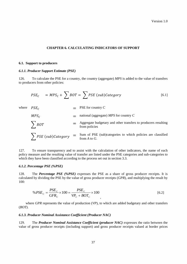
Version 1.0

37

CHAPTER 6. CALCULATING INDICATORS OF SUPPORT

6.1. Support to producers

6.1.1. Producer Support Estimate (PSE)

126. To calculate the PSE for a country, the country (aggregate) MPS is added to the value of transfers

to producers from other policies:

[6.1]

where PSE for country C

national (aggregate) MPS for country C

Aggregate budgetary and other transfers to producers resulting

from policies

Sum of PSE (sub)categories to which policies are classified

from A to G.

127. To ensure transparency and to assist with the calculation of other indicators, the name of each

policy measure and the resulting value of transfer are listed under the PSE categories and sub-categories to

which they have been classified according to the process set out in section 3.3.

6.1.2. Percentage PSE (%PSE)

128. The Percentage PSE (%PSE) expresses the PSE as a share of gross producer receipts. It is

calculated by dividing the PSE by the value of gross producer receipts (GPR), and multiplying the result by

100:

100100%

CC

C

C

CC

BOTVP

PSE

GFR

PSEPSE

,

[6.2]

where GPR represents the value of production (VP), to which are added budgetary and other transfers

(BOT).

6.1.3. Producer Nominal Assistance Coefficient (Producer NAC)

129. The Producer Nominal Assistance Coefficient (producer NAC) expresses the ratio between the

value of gross producer receipts (including support) and gross producer receipts valued at border prices

Version 1.0

38

(measured at edge of the producer‘s property).The producer NAC is calculated by dividing the value of

gross producer receipts by the value of production at border prices. Expressed algebraically:

CC

CC

MPSVP

GFRCproducerNA

[6.3]

The producer NAC is mathematically related to the %PSE, and can be alternatively derived as:

C

CC

PSE

PSECproducerNA

%100

%1

[6.4]

6.1.3. Producer Nominal Protection Coefficient (Producer NPC)

130. The Producer Nominal Protection Coefficient (producer NPC) expresses the ratio between the

average price received by producers (including payments for current output), and the border price,

measured at the producer‘s property. Producer NPC values may be calculated at the individual commodity

and national (aggregate) levels.

6.1.3.1. Producer NPC for individual commodities

131. The producer NPC for an individual commodity can be derived in two ways. First, domestic and

border prices can be compared, where the domestic price is the producer price plus the per unit transfers

received from payments based on output:

i

i

ii

iRP

QP

POPP

CproducerNP

[6.5]

where: iPP – producer price of commodity i

iPO – sum of payments to commodity i based on output (PSE sub-category A.2)

iQP – quantity produced of commodity i

iRP – reference price of commodity i

The numerator in equation 6.5 adds the payments based on output to producer price in order to

account for any direct supplements to producer price over and above market price support measures.

6.1.3.2. Producer NPC for a country

132. Once producer NPC values have been calculated for each individual commodity, a national

(aggregate) NPC can be derived. As prices and quantities cannot be aggregated for different commodities,

the producer NPC for a country is calculated using the value of transfers:

CCC

CCC

TPTTPCVP

POVPCproducerNP

[6.6]

where: CVP – total value of production for country C

Version 1.0

39

CPO – total sum of transfers in PSE category A.2 for country C

CTPC – total Transfers to Producers from Consumers for country C

CTPT – total Transfers to Producers from Taxpayers for country C

133. The producer NPC for individual commodities can also be calculated based on the transfer values

method, by substituting the appropriate values for the individual commodity into equation 6.6. When

expressed in this form it can be seen that the denominator for the producer NPC, while very close to, is

different from the denominator used to calculate the producer NAC (equation 6.4). The denominator for

the producer NAC subtracts the total MPS value from the value of production and not just transfers from

consumers and taxpayers to producer.

6.2. Support to consumers

6.2.1. Consumer Support Estimate (CSE)

134. The process of estimating a CSE begins by calculating a consumer single-commodity transfer

(SCT) value for each of the individual commodities for which MPS has been calculated.

[6.7]

where transfers to consumers from taxpayers for commodity i

transfers to producers from consumers of commodity i

other transfers from consumers of commodity i

135. TCT are budgetary payments to consumers (including tax concessions), to reduce the effective

price they have to pay for energy — e.g., to compensate them for the higher prices they pay for energy

products resulting from policies that support producer prices, to favour a particular industry, or to address

energy poverty. The TCT is obtained from the information on budgetary or tax expenditures. The sum of

the other two components in equation 6.7 corresponds to price transfers from consumers (PTC), which

include transfers both to domestic producers and (if some of the demand is met through imports subject to

an import tariff) to the government.

136. The information and analysis used to calculate market price support (MPS) is used as the basis

for carrying out these calculations — i.e. the same values for MPD, production, and consumption are used.

The TPC value is the mirror image of MPS for the same commodity. However, instead of being added as a

value transferred as support to producers, it is subtracted as a value transferred away from consumers. If

consumption is greater than production, then consumers also pay the MPD on the remaining volume of

consumption, supplied from imports (OTC).

137. Once consumer SCT values have been calculated for individual commodities, a national

(aggregate) CSE value can be calculated by a similar method:

[6.8]

Version 1.0

40

138. The national (aggregate) value of transfers to consumers from taxpayers is found by adding

together the value of TCT for all the individual commodities for which MPS has been calculated with any

additional TCT that are provided to consumers of non-MPS commodities, that is:

[6.9]

139.

6.2.2. Percentage CSE (%CSE) and Consumer Nominal Assistance Coefficient (Consumer NAC)

140. The %CSE for a country is calculated by dividing the CSE by the value of consumption

expenditure, i.e. value of consumption less transfers to consumers from taxpayers (TCT), and multiplying

the result by 100. Value of consumption is adjusted for TCT because it effectively reduces consumer

expenditure. This is expressed as:

[6.10]

where value of consumption of the sector in country C

141. The consumer NAC is calculated by dividing the value of consumption by the value of

consumption at border prices. Expressed algebraically:

[6.11]

142. The consumer NAC is mathematically related to the %CSE, and can be alternatively derived as:

[6.12]

6.2.3. Consumer Nominal Protection Coefficient (Consumer NPC)

143. As for the producer NPC, the consumer NPC indicator is first calculated at the individual

commodity level. The results are then used to derive a national (aggregate) consumer NPC.

144. The consumer NPC for an individual commodity is derived by comparing domestic and border

prices, where the domestic price is the consumer price. Note that the consumer price is normally equal to

producer price, which follows from the definition of consumer as a first-stage buyer of the commodity.

[6.13]

Version 1.0

41

Where consumer price of commodity i

sum of payments to consumers relating to their consumption of

commodity i

quantity consumed of commodity i

reference price of commodity i

145. As prices and quantities cannot be aggregated over a variety of different commodities, the

consumer NPC for a country is calculated based on the value of transfers:

[6.14]

where total value of production for country C

total Transfers to Producers from Consumers for country C

total Other Transfers from Consumers for country C

146. Note that the national (aggregate) consumer NPC can be lower or higher than the producer NPC

— depending on the relative size of the payments based on output received by producers, and payments

based on use received by consumers.

6.3. General Services Support and Total Support Estimate (TSE)

6.3.1 General Services Support Estimate (GSSE)

147. The GSSE measures the value of transfers provided through policies that support producers or

consumers collectively rather than as individuals. The GSSE can be estimated as:

[6.15]

Where General Services Support Estimate for country C

total value of transfers to GSSE category in country C

6.3.2 Total Support Estimate (TSE)

148. Two methods exist to calculate the TSE for a country, and both can be used to help to ensure that

all indicators of support are correctly calculated. The first method sums up the transfers distinguished by

recipient (i.e., transfers to producers, PSE), transfers to general services (GSSE), and transfers to

consumers from taxpayers (i.e. consumer subsidies, TCT):

Version 1.0

42

[6.16]

149. The second method sums up the transfers distinguished by source — i.e. transfers from

consumers (TPC + OTC) and transfers from taxpayers ((PSE – TPC) + GSSE + TCT – OTC) — as shown

in equitation 6.16 (algebraically it can be reduced to equation 6.15):

[6.17]

150. It should be noted that both methods for calculating the TSE involve the assumption that the total

value of transfers from consumers to others (OTC) is received as budget revenue (e.g., as import duties).

6.3.3 Percentage GSSE (%GSSE) and the percentage TSE (%TSE)

151. Two relative indicators of support are derived from absolute values of GSSE and TSE. The

%GSSE indicates the importance of support to general services within total support. It is calculated as the

percentage share of the TSE:

[6.18]

152. The %TSE indicates the level of total support to a sector relative to a country‘s gross domestic

product (GDP). The %TSE is found as a percent share of the value of GDP:

[6.19]

6.4. Calculating indicators of support for groups of countries or for the world

6.4.1. Conversion into a common currency

153. To obtain total support indicators for a group of countries, or for the world, the value of transfers

and production in national currencies must be converted into a common currency. The choice of the

common currency has an important impact on the results in terms of how the absolute indicators: (a)

compare between countries, and (b) change from year to year. For this reason, it is advisable to convert all

support indicators in both US dollars and another common currency, such as the euro. However, the

relative indicators among countries in a given year will not be changed by the choice of a common

currency.

6.4.1. Aggregation to regional or global totals

154. Once the values of transfers and production have been converted into a common currency, or

currencies, aggregation into global totals can be carried out.

Version 1.0

43

CHAPTER 7. DATA AND INFORMATION REQUIREMENTS FOR CALCULATING THE

INDICATORS

155. This chapter lists the data and information requirements for calculating indicators of support,

drawing on the methodology detailed in the previous chapters of Part II. Its purpose is to assist those

involved in calculating indicators in gathering the necessary information which may be needed from a wide

range of sources.

156. The indicators are calculated on an annual basis. The time scale (i.e. the number of years) over

which the indicators are calculated will, accordingly, increase the quantity of information required.

7.1. Requirements for calculating price transfers

157. Information required on the domestic market:

Value and volume of production information for individual commodities and (if of interest) total

energy at the producer level.

Producer prices, clearly indicating the unit that it is based on. For consistency within the transfer

calculation, either the value of production is found by multiplying quantity by price, or

alternatively the value is divided by quantity to derive a producer price.

Consumption data are also required. This can be obtained directly, or as a result of adding the

volume of production and imports and subtracting imports, ensuring that the same product weight

basis is used.

158. Sources that can be used to obtain information related to marketing margins include:

Estimations published by national authorities. However, such data are relatively rare, since the

information is often commercially sensitive.

Estimations obtained on a regular but often ad hoc basis from national authorities, industry

organisations or major private companies.

Estimating the marketing margin as the difference between the producer price and an average

wholesale price in the country considered. However, this type of estimation leads to very variable

margins, and it may be appropriate to use a moving average margin for several years. This option

is less preferable than the previous two.

Using marketing margins available in other countries if no domestic information is available.

159. Trade data include:

Values and volumes for both exports (FOB) and imports (CIF) of energy commodities and

products.

Version 1.0

44

Tariff schedule for the country – to understand the profile of tariffs imposed on imports.

Export subsidy budgetary information (if applicable).

Exchange rates – information on official exchange rates, on an annual basis, and, if relevant, on a

monthly basis so that any seasonal calculations can be made.

7.2 Requirements for calculating budgetary and other transfers

160. Data on budgetary transfers related to the implementation of energy policies are typically based

on official budgetary information on the execution of national budgets and reports by relevant agencies.

The majority of this information is publicly available on the internet sites of the ministries of finance,

energy and central banks of the countries concerned. Administrative databases which provide detailed

information on current expenditures by programmes also exist within the ministries, often on a monthly

basis. These help to adequate allocation of payments to calendar years. However, this information is not

usually publicly available.

161. Care should be exercised when budgetary information is compiled from several sources. Some

sub-national expenditures may be reported both independently and as part of the expenditures made at

higher administrative levels. Another case warranting caution in order to avoid double-counting is where

data on the budgetary outlays are compiled through combination of sources reporting the public spending

by agencies and by specific programmes or activities. It is generally preferable to use a single source of

budgetary information; however, this does not often provide sufficient detail on the budgetary spending,

thus making it necessary to use several sources. It is therefore important to understand the composition of

the budgetary data reported in various sources used.

162. Estimation of support based on revenue foregone demands recourse to official documents

describing the relevant mechanisms. For example, to estimate transfers related to preferential lending,

official documents (regulations) are required describing the conditions of lending, including time terms of

loans, repayment schedules and interest rates applied. In the case of debt rescheduling, all relevant

government decisions outlining the conditions and schedules for repayments should be used. Information

on preferential interest rates is usually available from the relevant Ministry and banks involved in

preferential lending. Information on market (reference) interest rates is usually published by the central

banks. Ministries and agencies dealing with macro-economic issues typically provide various price and

financial data.

163. Support based on revenue foregone presents a particular difficulty in terms of achieving

consistency across countries (e.g. as is the case of tax concessions) because these transfers are not always

measured or reported.

Version 1.0

45

GLOSSARY

Conditional loan: An official loan that is to be reimbursed only if the project financed with the loan turns

out to be commercially successful. If the project fails, the loan is not reimbursed — i.e., it becomes a

grant. Conditional loans usually carry an interest and appear as a credit liability in the borrowing

company‘s balance sheet.

Forgivable loan: A loan which the lender undertakes to waive repayment of under certain prescribed

conditions. A conditional loan is a specific example of a forgivable loan.

Interest-rate subsidy: A subsidy to the interest cost of a loan borrowed from a private loan institution.

Interest-rate subsidies are typically offered to certain specific sectors, for certain types of

investments and uses, or certain sizes of companies.

Reimbursable grant: A government grant, in general for R&D and innovation in a new product, that is to

be reimbursed by the beneficiary if the project turns out to be commercially successful. In general,

there is no additional interest cost included in these reimbursements.

Version 1.0

46

REFERENCES

Asian Development Bank (1997), Guidelines for the Economic Analysis of Projects, Asian Development

Bank, Manila, Philippines. www.adb.org/Documents/Guidelines/Eco_Analysis/eco-analysis-

projects.pdf

Baig, T., A. Mati, D. Coady, and J. Ntamatungiro (2007), ―Domestic Petroleum Product Prices and

Subsidies: Recent Developments and Reform Strategies‖, IMF Working Paper 07/71, International

Monetary Fund, Washington, D.C.

Briceño-Garmendia, Cecilia, Karlis Smits and Vivien Foster (2008), ―Financing Public Infrastructure in

Sub-Saharan Africa: Patterns and Emerging Issues‖, Africa Infrastructure Country Diagnostic,

Background Paper 15, World Bank, Washington, D.C.

Bruce, Neil (1990), Measuring Industrial Subsidies: Some Conceptual Issues‖, OECD Economics

Department Working Papers, No. 75, OECD Publishing, Paris. Doi:10.1797/781417028471

Coady, D., M. El-Said, R. Gillingham, K. Kpodar, P. Medas and D. Newhouse (2006), ―The Magnitude

and Distribution of Fuel Subsidies: Evidence from Bolivia, Ghana, Jordan, Mali, and Sri Lanka,‖

IMF Working Paper 06/247, International Monetary Fund, Washington, D.C.

Coady, David, Robert Gillingham, Rolando Ossowski, John Piotrowski, Shamsuddin Tareq, and Justin

Tyson (2010), ―Petroleum Product Subsidies: Costly, Inequitable,and Rising‖, IMF Staff Position

Note No. SPN/10/05, 25 February 2010, International Monetary Fund, Washington, D.C.

Corden, W.M. (1971), The Theory of Protection, Oxford University Press, London.

Desai, V.V. and J. Lee (1997), ―Bank criteria for subsidies‖, unpublished manuscript, Asian Development

Bank, Manila, Philippines. www.adb.org/Documents/Policies/bank-criteria/bank-criteria-for-

subsidies.pdf

Donohue, Michael (2008), Environmentally Harmful Subsidies in the Transport Sector, OECD Document

No. ENV/EPOC/WPNEP/T(2007)1/FINAL, OECD, Paris.

Ebinger, Jane O. (2006), ―Measuring Financial Performance in Infrastructure: An Application to Europe

and Central Asia‖, World Bank Policy Research Working Paper No. 3992, World Bank,

Washington, D.C.

Ford, Robert and Wim Suyker (1990), ―Industrial subsidies in the OECD Economies‖, OECD Economics

Department Working Papers, No. 74, OECD Publishing, Paris. doi:10.1787/062357858637

IASB (International Accounting Standards Board) (2009), International Accounting Standard 20:

Accounting for Government Grants and Disclosure of Government Assistance, IASB, London.

IEA (International Energy Agency) (1988), Coal Prospects and Policies in IEA Countries, OECD

Publications, Paris.

Version 1.0

47

IEA (1999), ―Looking at Energy Subsidies: Getting Energy Prices Right‖, World Energy Outlook,

OECD/IEA, Paris.

IEA (2001), Coal Information 2001, OECD/IEA, Paris.

IEA (2006 and 2008), World Energy Outlook, OECD/IEA, Paris.

Looney, Robert (1999), ―Subsidies‖, in R.J.B. Jones (ed.), Routledge Encyclopedia of International

Political Economy, Routledge, London. http://web.nps.navy.mil/~relooney/Routledge_54.htm

Plunkett, H., R. Wilson and S. Argy (1992), ―The Measurement of Effective Rates of Assistance in

Australia‖, Working Paper No. 4, Industry Commission, Belconnen, ACT, Australia.

www.pc.gov.au/__data/assets/pdf_file/0007/93427/measurement-effective-rates-assistance.pdf

OECD (1995), Industrial Subsidies: A Reporting Manual, OECD Publishing, Paris.

OECD (2009), OECD’s Producer Support Estimate and Related Indicator of Agricultural Support:

Concepts, Calculations, Interpretation and Use (The PSE Manual), OECD Publishing, Paris.

OECD (2010), Tax Expenditures in OECD Countries, OECD Publishing, Paris.

Saavalainen, Tapio and Joy Ten Berge (2006), ―Quasi-Fiscal Deficits and Energy Conditionality in

Selected CIS Countries‖, IMF Working Paper No. 06/43, International Monetary Fund, Washington,

D.C.

Steenblik, Ronald P. (1995), ―A note on the concept of `subsidy',‖ Energy Policy, Vol. 23, Issue 6, Coal in

Europe: implications of dismantled subsidies (Marian Radetzki, ed.), June 1995, pp. 483-484.

Steenblik, R. (2003), ―Subsidy measurement and classification: developing a common framework‖,

Chapter 3 in Environmentally Harmful Subsidies: Policy Issues and Challenges, proceedings of the

OECD Workshop on Environmentally Harmful Subsidies (Paris, 7-8 November 2002), OECD

Publications, Paris, 2003, pp. 101-141.

Steenblik, Ronald P. and P. Coroyannakis (1995), ―Reform of coal policies in Western and Central Europe:

Implications for the environment,‖ Energy Policy, Vol. 23, Issue 6, Coal in Europe: implications of

dismantled subsidies (Marian Radetzki, ed.), June 1995, pp. 537-553.Hamsvoort, C.P.C.M. van der

(1994), ―PSE as an Agregate Measure of Support in the Uruguay Round‖, Research Paper No. 122,

Agricultural Economics Research Institute, The Hague.