Measuring Systematic Risk Using Implied Beta in Option … ANNUAL MEETINGS/2011-… · Measuring Systematic Risk Using Implied Beta in ... portfolio with a desired level of the

0

Measuring Systematic Risk Using Implied Beta in Option Prices

January 10, 2011

Bing-Huei Lin* Department of Finance

National Chung Hsing University 250 Kuo Kuang Road, Taichung 402, Taiwan

TEL: +886-4-22840808 FAX: +886-4-22856233

Email: [email protected]

Dean Paxson Manchester Business School

University of Manchester Email: [email protected]

Jr-Yan Wang Department of International Business

National Taiwan University Email: [email protected]

Mei-Mei Kuo Department of Business Administration

National Taiwan University of Science and Technology Email: [email protected]

EFM Classification Codes: 310

* The corresponding author will attend and present in the conference.

1

Measuring Systematic Risk Using Implied Beta in Option Prices

ABSTRACT

This paper provides a novel method to estimate β thoroughly based on option prices. Through combining the market model and the multivariate risk-neutral valuation relationship in Stapleton and Subrahmanyam (1984) and Câmara (2003), we develop a pricing model for individual stock options involving the volatility of the market index level and the levels of the β and the idiosyncratic risk of the underlying stock asset. Based on this option pricing model, it is possible to estimate β implicitly from the current prices of index options and individual stock options rather than from the historical stock prices in the traditional method. The proposed option pricing model can explain some aspects of volatility smiles and term structures. The empirical studies for the component stocks in Dow Jones Industrial Average (DJIA) show that the option-implied β from this novel method can provide reasonable estimates of β and perform better than historical β in predicting the realized value of β in future periods of time. Furthermore, the results of the competitive regression suggest that the option-implied β contains the information different from that in the historical β.

2

I. Introduction

In order to estimate the forward-looking β, this paper develops a pricing model for

individual stock options involving the volatility of the market index level and the

levels of the β and the idiosyncratic risk of the underlying stock asset. Equipped with

this novel model, we are able to estimate β for a future period of time purely based on

the current prices of index options and individual stock options. Since the seminal

work of Capital Asset Pricing Model (CAPM) in Sharpe (1964) and Lintner (1965),

the systematic risk and its measurement β are the standard textbook measure of risk.

The CAPM and the information of β are commonly used in finance, for instance in

calculating the cost of capital, pricing the value of investments, or constructing a

portfolio with a desired level of the systematic risk. Although CAPM has been

subject to some criticisms (e.g., Roll (1977) and Fama and French (1992)), CAPM

remains well on the frontier of both academic research and industry applications.

Thus, pursuing accurate estimates of β, in particular for future periods of time, is an

important issue for so long.

Although the information of β should reflect the sensitivity of the individual

stock return to the return of the market portfolio for a future period of time, it is

unobservable and estimated from a backward viewpoint traditionally, i.e., using

historical excess returns of the individual stock and the market portfolio to estimate

the β of an asset based on the regression model. This method was first proposed by

Jensen (1968), who noted that the Sharpe-Lintner version of the linear relation

between expected excess returns and the β also implies a regression test. It is known

as the market or single-index model which takes the following form:

, , , , , ,

where , , and , , are the excess returns on the asset i and the

3

market portfolio at time t, respectively. The random variable , is a white noise and

independently identical distributed over time. The coefficients and are

constant parameters to be estimated. Under the normal assumptions, the ordinary

least squares method provides unbiased estimates for and . The level of

assesses the impact of the price changes in the market portfolio on the price changes

in asset i. The CAPM implies that the intercept term in the regression, also

termed “Jensen’s alpha,” should be zero for any asset.

This traditional backward-looking method to estimate (or to extrapolate) the

future β may not perform well unless the patterns of beta are known and stable in the

near future. However, numerous studies find that violations of the assumption of

stationarity and independently identical distributed returns are rules rather than

exceptions, such as Blume (1971, 1975), Baesel (1974), Klemkosky and Martin

(1975), Roenfeldt, Griepentrog, and Pflaum (1978), Fabozzi and Francis (1978),

Theobald (1981), Bos and Newbold (1984), Collins, Ledolter, and Rayburn (1987)

and Faff, Lee, and Fry (1992). Moreover, when firms are involved in some events,

like mergers or acquisitions, undertaking large-scale projects, or changing their

capital structure, historical returns cannot provide adequate information to estimate

the future β reliably. Although there are several financial econometric models to

remedy this problem,1 it is difficult to assess the bias associated with the estimation

of ex ante information using ex post historical data.

To estimate the future β, some authors combine the implied volatilities from

option prices and the historical correlation of individual equity and equity index

prices, e.g., French, Groth, and Kolari (1983). However, a radically different

1 For instance, the conditional beta or other time-varying models of beta are considered in Ferson,

Kandel, and Stambaugh (1987), Jagannathan and Wang (1996), Ferson and Harvey (1999), Park (2004), Fraser, Hamelink, Hoesli, and Macgregor (2004), and Adrian and Franzoni (2009).

4

methodology to estimate a forward-looking beta based on option prices is first

introduced by Siegel (1995). Given the implied volatilities of the individual stock and

the market portfolio, he exploits the option valuation model for exchange options

developed in Margrabe (1978) to price an option which exchanges the individual

stock return to the market index return and thus can calibrate the β from option prices.

The core of Siegel’s model depends on the existence of that kind of exchange option

traded in the market. However, that kind of exchange option is not generally available

in the market, so Siegel’s method to estimate β is not practical.

There are several empirical studies, such as Bates (1998), Buraschi and

Jackwerth (2001), Dennis and Mayhew (2002), and Bakshi, Kapadia, and Madan

(2003), demonstrating the existence of systematic risk factors in option prices.

Therefore, some academics try to extract the market beta from option prices.

Husmann and Stephan (2007), extending the model in Jarrow and Madan (1997)

to price stock index options in an incomplete market, introduce an option pricing

formula for individual equity options based on the CAPM so that the value of β can

be estimated implicitly from the current market prices of individual equity options.

However, since their model do no rely on the risk neutral valuation method, in

addition to the correlation (or the β) parameter, there are other risk preference

parameters in their option pricing formula, such as the expected returns of the

individual stock as well as the market portfolio. Chen, Kim, and Panda (2009) and

Chang, Christoffersen, Jacobs, and Vainberg (2010) also estimate the β from current

option prices. To estimate option-implied β for a future period of time, Chen et al.

(2009) derive the counterpart of the Black-Scholes formula under the physical

measure and then links the expected returns of the underlying stock and the option

with a single-index model. It is unavoidable that they require the expected stock

return, which is preference-dependent, in their option pricing formula. Chang et al.

5

(2010) extend the method in Bakshi, Kapadia, and Madan (2003), which studies the

relationship between the option-implied variance and skewness of the underlying

asset return. However, this stream of models ignores that the possible conflict

between the assumptions of the normal distribution in CAPM and the existence of

skewness in stock returns.

Building on Siegel (1995) and Husmann and Stephen (2007), we propose a new

method to estimate β purely based on quoted option prices. The core of this new

method is to develop an option pricing model by combining the market model with

the multivariate risk-neutral valuation relationship (RNVR) in Stapleton and

Subrahmanyam (1984) and Câmara (2003). The RNVR is a very useful technique for

asset pricing, especially for derivatives whose payoffs are determined by one or

several underlying variables, whether traded or non-traded. The RNVR-based models

exploit simply the relationship between derivatives and their underlying assets to

derive the preference-free derivative pricing formula. As a consequence, the

preference parameters are not involved in the valuation equation of the derivatives,

and the expected return on the underlying assets is the riskless return.

The RNVR was first developed by Rubinstein (1976) and Brennan (1979) for

derivatives pricing when there is only one underlying variable. Under the sufficient

conditions that there is a representative agent whose risk preference is with an

exponential representation, and his period-end wealth and the underlying asset price

are jointly normally distributed, the RNVR can generate a preference-free option

pricing formula, which could be identical to the formula in Black and Scholes (1973).

Stapleton and Subrahmanyam (1984) extend the model in Brennan (1979) by

allowing for multiple underlying variables. More recently, Câmara (2003) provides a

generalized RNVR framework to encompass a family of bivariate transformed

normal distribution for the period-end wealth and the underlying asset price to price

6

derivatives. The transformed normal distributions considered in Câmara (2003)

include the normal, lognormal, displaced lognormal, negatively skew lognormal, and

SU distributions. Câmara (2005) expands Câmara (2003) to a multivariate setting. By

considering the multivariate transformed normal distribution, Câmara’s method

contributes substantially to the literature to provide different risk-neutral option

pricing formulae with different preferences and alternative joint distributions of the

state variables.

In comparison with the continuous time option pricing model proposed in Black

and Scholes (1973), the discrete time RNVR-based model is less popular. However,

Black and Scholes only assume that investors prefer more wealth to less but assume

nothing about the risk preference of an investor. In contrast, the RNVR approach is

based on the market equilibrium rather than on the no-arbitrage argument in the

Black and Scholes framework. Therefore, the RNVR approach is highly general and

useful in asset pricing especially when additional assumptions are imposed on the

model. Our option pricing model is based on the RNVR approach together with the

assumption that returns of individual stocks follow the market model.

We consider a general exponential form of marginal utility function for the

representative agent and transformed normal distributions for state variables.

Additionally, according to the market model, the return of the individual stock is

assumed to be the sum of the market risk premium and an idiosyncratic risk

component. Thus, the two state variables in the RNVR are the market index return

and the idiosyncratic risk component of the individual stock. Finally, a

preference-free pricing model for individual stock options is derived, based on the

volatility of the market index level and the levels of the β and the idiosyncratic risk of

the underlying stock asset. This novel option pricing formula enables the estimation

of β purely based on prices of stock index and individual stock options. This paper

7

not only provides an alternative to estimating β but is the first model to estimate β in

a purely forward-looking way based only on quoted option prices.

The remainder of this paper is organized as follows. Section II presents the

framework of multivariate risk-neutral valuation relationship. Section III is devoted

to derive an explicit risk-neutral option pricing model for European calls and discuss

the relationship between the implied volatility smiles or term structures and the levels

of the β and the idiosyncratic risk of the individual stock. Section IV presents the

empirical results of this paper, including the description of the data of option prices,

the introduction of the calibration procedures, and the analysis of the calibrated

results. Section V concludes this paper.

II. The General Multivariate Risk-Neutral Valuation Relationship

In a one-period economy, for the case of multiple underlying processes, the standard

pricing relationship for derivatives considered in Brennan (1979), Stapleton and

Subrahmanyam (1984), and Câmara (2003) is

· , (1)

where is the price of a derivative contract today, Rf is the gross return of the

risk-free asset for the examined period, and · stands for the expectation operator

under the actual probability measure. The variable X is a vector of payoffs of n

underlying processes and , , … , C(X) is the payoff function for the

derivative contract, and is the asset-specific pricing kernel. Following Câmara

(2003), the definition of is given by:

, (2)

8

where is the marginal utility function of the wealth of the representative agent on the maturity date.

In addition, the period-end wealth, w, is assumed to follow a transformed normal

distribution:2

~ , ,

where and are the mean and variance of , and (·) is a strictly

monotonic and differentiable function. Following the method in Câmara (2003) to

generalize the Brennan-Rubinstein approach for pricing derivatives, we assume that

the representative agent’s marginal utility is of the exponential form:

exp ,

where α is a constant preference parameter. As a consequence, it is straightforward to

infer that ln ~ , . Câmara (2003) argues that the exact functional

form of · is not critical as long as is normally distribution. For example,

if the period-end wealth is normally distributed, exp given

should be considered, which implies that the representative agent has

constant absolute aversion; it is a necessary condition to derive the RNVR for a

bivariate normal distribution of the price of the underlying assets and period-end

wealth. On the other hand, if the period-end wealth follows a lognormal distribution,

the representative individual’s marginal utility is a power function, that is

given ln , which implies that the representative agent is with

constant proportional aversion; it is a necessary condition to derive the RNVR for a

2 The definition of the transformed normal random variable is that a random variable Y can be

expressed as , where ~ 0,1 , and f is a strictly monotonic differentiable

function.

9

bivariate lognormal distribution of the price of the underlying assets and period-end

wealth.

As to the underlying assets or state variables, we assume the joint distribution of

the underlying assets at the end of the period to be a multivariate transformed normal

distribution:

, , … , ~ , ,

where µ and are the mean vector and the variance-covariance matrix of the

underlying multivariate normal distribution, and hi’s are arbitrarily strictly monotonic

and differentiable functions. The probability density function of the underlying assets

, , … , is:

, , … , ⁄ | | ⁄ | |exp . (3)

In addition, the wealth of the representative agent and the underlying asset prices

at the end of the period are further assumed to follow a jointly transformed normal

distribution. Therefore, the conditional distribution of the representative agent’s

marginal utility is

ln | ~ , ,

where is a row vector representing the covariances between ln and .

According to the property of the lognormally distribution, it is straightforward to

drive | and . As a result, the pricing kernel is

expressed as

exp α . (4)

10

Substituting Equations (3) and (4) into Equation (1), the derivative valuation

formula becomes as follows.

⁄ | | ⁄ | |

· exp … , (5)

and the current price of the underlying assets P is

… ⁄ | | ⁄ | |

· exp … , (6)

where the location parameter of the density of the underlying assets is a

preference-related term . Under the market equilibrium, if the expectation

of Equation (6) has an inverse function for its location parameter , then the

resulting expression can be substituted into Equation (5), i.e., can be

replaced by a function of · . As a consequence, the probability density function

of without preference parameters can be derived, and thus the price of the

derivative can be written as a preference-free option pricing equation:

,

where · denotes the expectation under the risk-neutral probability measure Q.

Since the location parameter is a function of in the corresponding risk-neutral

probability density function of X, it is consistent to the classic option pricing theory

that to price derivatives in the risk-neutral world, the expected returns of all assets are

equal to the riskless return. In the next section, we will apply this RNVR method to

11

the pricing of individual stock options by incorporating the market model to

formulate the return of the underlying stock price.

III. The Option Pricing Model Involving β

III.1 Distributions of Underlying Variables and the Aggregate Wealth

In the case of pricing individual stock options, we consider two points of time–today

is time 0 and the maturity date of the option is time T. Taking European call options

as examples,3 the payoff at the time point T is

max , 0 .

In addition, according to the market model, we can transform the payoff of the equity

call option into a multivariate function of the market index return and an idiosyncratic

risk component. That is

max , 0

· max , 0 · max , 0

· max 1 , 0

, , (7)

where ST is the stock price at time T, S0 is the stock price at time 0, and k is defined as

K/S0. In addition, RT≣ST/S0 is the gross return on the underlying stock, Rf is the

gross return of the risk-free asset between time 0 and time T, and Rm is the gross

3 As for individual put options, it is straightforward to derive the counterpart option pricing formulae

by simply considering the payoff of put options in Equation (7) and following the same procedure mentioned as follows.

12

return on the market portfolio from time 0 to time T and assumed to follow a

lognormal distribution, i.e., ln ~ , , where is the annualized

expected return of the market portfolio, and is the variance of the annualized

market index return. The idiosyncratic (or firm-specific) risk component re associated

with the underlying individual stock is assumed to follow 0, , where the

expected return on the idiosyncratic risk component is zero by definition, and is

the corresponding annual variance for the idiosyncratic risk component. Finally,

, where q is the annualized dividend yield, reflecting the decline of the

stock price due to dividend payments .

Following the RNVR approach introduced in Section II, we assume that the

period-end wealth of the representative agent w, the gross return on the market

portfolio Rm, and the idiosyncratic risk component re follow the trivariate transformed

normal distribution as follows.

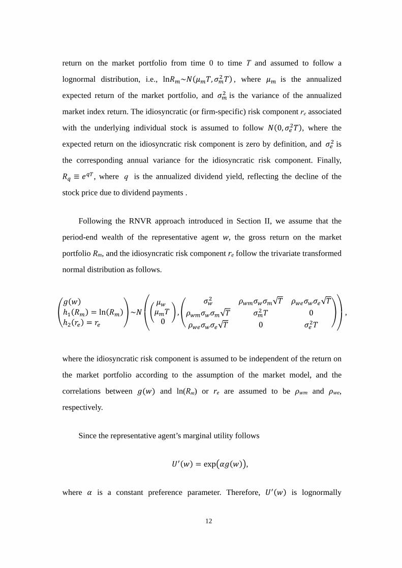
ln ~

0

,√ √

√ 0√ 0

,

where the idiosyncratic risk component is assumed to be independent of the return on

the market portfolio according to the assumption of the market model, and the

correlations between and ln(Rm) or re are assumed to be ρwm and ρwe,

respectively.

Since the representative agent’s marginal utility follows

exp ,

where is a constant preference parameter. Therefore, is lognormally

13

distributed with the mean αμw and the variance . Consequently, the mean of

this lognormal random variable is

exp .

Furthermore, since

ln | , ~√

ln√

0 ,

1 ,

we can obtain that

| , exp√

ln√

0

1 .

Following Equation (2), we can obtain the asset-specific pricing kernel

, as follows.

, | , exp√

ln√

0

8

III.2 The Risk Neutral Valuation Relationship

According to the assumption about the return on the market portfolio and the

idiosyncratic risk component following a bivariate transformed normal distribution

by setting ln and , we can derive 1⁄ and

1 and rewrite Equation (3) as follows.

14

,√ √

exp ln ·

√ √

exp 0 . 9

Given the density of , in Equation (9) and the asset-specific pricing

kernel , in (8), the option pricing formula (5) can be rewritten as:

,√ √

· exp ln √ ·

√ √exp 0 √ . (10)

According to Equation (6), we can obtain the present value for the market portfolio

return and the idiosyncratic risk component to be

·√ √

· exp ln √

·√ √

exp 0 √ .

The current prices of the underlying variables Rm and re, which are the return on

the market portfolio and the idiosyncratic risk component for the individual stock, are

1 and 0 by definition. Hence

1

0exp √

0 √.

Then we can obtain the following relationship:

15

√0 √

ln0

. (11)

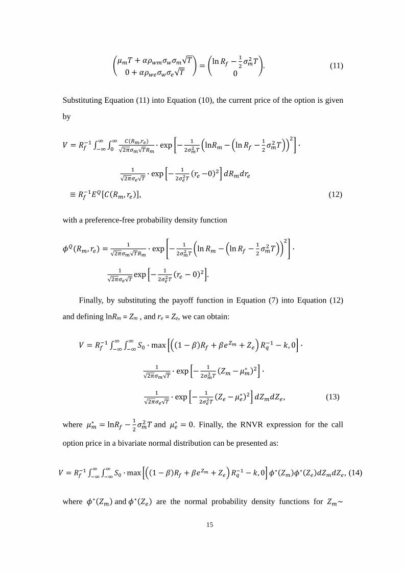
Substituting Equation (11) into Equation (10), the current price of the option is given

by

,√ √

· exp ln ln ·

√ √· exp 0

, , (12)

with a preference-free probability density function

,√ √

· exp ln ln ·

√ √

exp 0 .

Finally, by substituting the payoff function in Equation (7) into Equation (12)

and defining lnRm = Zm , and re = Ze, we can obtain:

· max 1 , 0 ·

√ √

· exp ·

√ √

· exp , (13)

where ln and 0. Finally, the RNVR expression for the call

option price in a bivariate normal distribution can be presented as:

· max 1 , 0 , (14)

where and are the normal probability density functions for ~

16

ln , and ~ 0, .

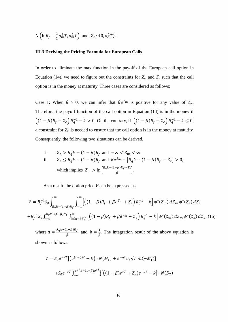
III.3 Deriving the Pricing Formula for European Calls

In order to eliminate the max function in the payoff of the European call option in

Equation (14), we need to figure out the constraints for Zm and Ze such that the call

option is in the money at maturity. Three cases are considered as follows:

Case 1: When β > 0, we can infer that is positive for any value of Zm.

Therefore, the payoff function of the call option in Equation (14) is in the money if

1 0. On the contrary, if 1 0,

a constraint for Zm is needed to ensure that the call option is in the money at maturity.

Consequently, the following two situations can be derived.

i. 1 and ∞ ∞. ii. 1 and 1 0,

which implies ln .

As a result, the option price V can be expressed as

1

1 , (15)

where and . The integration result of the above equation is

shown as follows:

· √ ·

1 ·

17

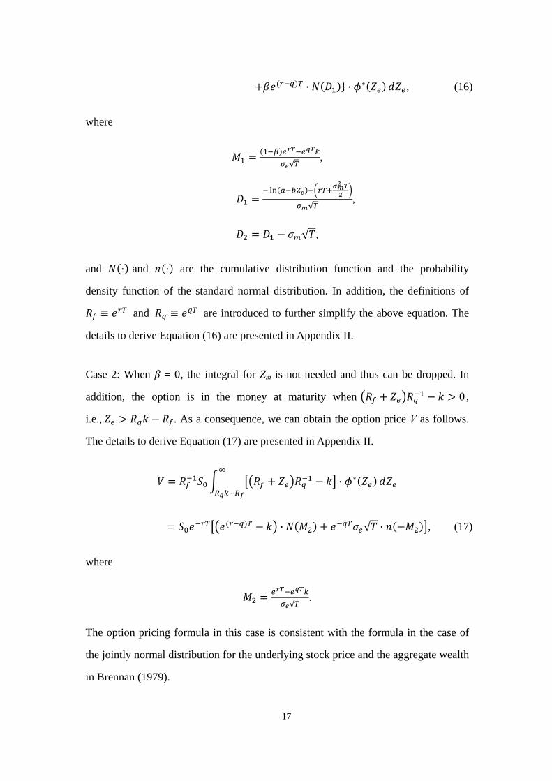
· · , (16)

where

√,

√

,

√ ,

and · and n · are the cumulative distribution function and the probability

density function of the standard normal distribution. In addition, the definitions of

and are introduced to further simplify the above equation. The

details to derive Equation (16) are presented in Appendix II.

Case 2: When β = 0, the integral for Zm is not needed and thus can be dropped. In

addition, the option is in the money at maturity when 0 ,

i.e., . As a consequence, we can obtain the option price V as follows.

The details to derive Equation (17) are presented in Appendix II.

·

· √ · , (17)

where

√.

The option pricing formula in this case is consistent with the formula in the case of

the jointly normal distribution for the underlying stock price and the aggregate wealth

in Brennan (1979).

18

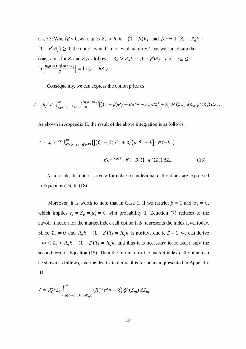
Case 3: When β < 0, as long as 1 , and

1 0, the option is in the money at maturity. Thus we can obtain the

constraints for Ze and Zm as follows: 1 and

ln ln .

Consequently, we can express the option price as

1 .

As shown in Appendix II, the result of the above integration is as follows.

1 ·

· · . (18)

As a result, the option pricing formulae for individual call options are expressed

in Equations (16) to (18).

Moreover, it is worth to note that in Case 1, if we restrict β = 1 and 0,

which implies 0 with probability 1, Equation (7) reduces to the

payoff function for the market index call option if S0 represents the index level today.

Since 0 and 1 is positive due to β = 1, we can derive

∞ 1 , and thus it is necessary to consider only the

second term in Equation (15). Then the formula for the market index call option can

be shown as follows, and the details to derive this formula are presented in Appendix

III.

·

19

·√

· ·√

·√

·√

, (19)

which is identical to the Black-Scholes formula. The above result demonstrates the

Black-Scholes formula is a special case of our model when β = 1 and σe = 0, and for

pricing market index call options, our model is equivalent to the classic

Black-Scholes model.

Finally, the pricing formulae in Equations (16) and (18) are semi-analytical

solutions and should be computed with numerical techniques. For the remaining

integral over Ze, we exploit the Gaussian quadrature method to complete the

computation of option prices. In our computer program, 2000 points are considered in

the Gaussian quadrature method, and the option prices converge within 10–7, which

guarantees that option prices generated through our model converge to the theoretical

ones. In addition, the speed of our computer program is also fast. It takes less than 0.1

second to compute each option price.

III.4 Implied Volatility Smiles Based on Our Model

Under the Black-Scholes model, the risk-neutral probability density function of the

underlying price is a lognormal distribution with a constant volatility. However, this

pattern has been convincingly rejected (see, for example, Macbeth and Merville

(1979) and Rubinstein (1985)). In the literature, there are in general two ways to

remedy this problem. The first way is to develop alternative stochastic processes,

which in turn imply risk-neutral densities more similar to the implied risk-neutral

20

density from the market prices of options. The other way is to extract implied

risk-neutral densities from option prices in markets directly (e.g., Rubinstein (1994)).

Many existing studies, like Jackwerth (2000), Dennis and Mayhew (2002), and

Bakshi, Kapadia, and Madan (2003), have found that implied risk-neutral densities

tend to be more negatively skewed than the lognormal density, which is the reason for

the implied volatility smiles and term structures.

The model proposed in this paper provides an alternative explanation for the

causation of the implied volatility smiles and term structures. We find that the levels

of the β and the idiosyncratic risk can influence the implied volatility smile, and this

effect diminishes for options with longer time to maturities.

Table 1 and its corresponding Figure 1 report the implied volatilities of option

values calculated by our model given different combinations of the values of beta and

the strike price. The values of other parameters in the base example in Table 1 are as

follows: the current stock price S0 is $50, the risk-free rate r is 0.1, the dividend yield

q is 0, the time to maturity T is 1, the volatility of the market index level σm is 0.15,

the idiosyncratic volatility σe is 0.3, and the examined strike prices are from $30 to

$70 with an increment of $5. For each result in Table 1, we compute the option values

via our model first, and next derive the corresponding implied volatilities based on

the Black-Scholes model. The slope of the implied volatility curve is defined as

– / (30 – 70), where IV is the abbreviation of implied volatility. For

example, the slope for β = 0.25 is –0.0031, which is obtained from (0.3682 – 0.2436)

/ (30 – 70). By observing the slope for the implied volatility curve of each β, we find

that the implied volatility curves are with more negatively slopes for higher values of

β than lower values of β. In other words, the implied volatility smile phenomenon is

more significant for the underlying asset with a higher level of the systematic risk.

21

Our results are consistent with those found in Duan and Wei (2009). They find that a

higher degree of systematic risk leads to higher implied volatilities and a steeper

slope of the implied volatility curve. In fact, the option pricing model proposed in this

paper is the first to incorporate this feature found in the empirical data.

Based on the same example in Table 1, we further analyze how the level of the

idiosyncratic risk affects the implied volatility smile by examining σe to be 0.2 and

0.4. The corresponding implied volatility curves are shown in Table 2 and Figure 2.

We find that the implied volatility smile is more pronounced for higher levels of the

idiosyncratic risk, e.g., when β equals 1.5, the slopes of the implied volatilities curves

are –0.00256 for σe = 0.2 and –0.00470 for σe = 0.4. To the best of our knowledge, we

are the first to find that the level of the idiosyncratic risk could affect the slope of the

implied volatility curve.

Based on the results in Tables 1 and 2, we conclude that the volatility smile

phenomenon is more significant for higher levels of β and the idiosyncratic risk σe.

Note that instead of focusing on studying the direct relationship between the negative

skewness and the negative slope of the implied volatility curve, such as the methods

in Jackwerth (2000), Dennis and Mayhew (2002), and Bakshi, Kapadia, and Madan

(2003), this paper develops an option pricing model that explicitly incorporates the β

and the idiosyncratic risk component under the lognormal (or normal) distribution

and concludes that the higher levels of the β and the idiosyncratic risk could generate

implied volatility curves with more negative slopes. If the negative skewness is the

only reason for the negative slope of the implied volatility curve, then our results

suggest that option traders may already consider the systematic risk and the

idiosyncratic risk of the underlying stock when estimating option values, and this

behavior may be the reason for the negative skewness of the risk-neutral distribution

22

of the underlying stock price.

It is well-known that the implied volatility curve changes with the time to

maturity. Based on the same example in Table 1, we further examine the implied

volatility curves for the different time to maturity T. The results of T = 0.25 and T = 2

are presented in Table 3 and Figure 3, which suggest that the volatility grin effect

decays with the increase of the time to maturity. Our results are reconciled with the

results of many previous studies, such as Backus, Foresi, and Wu (2004) and Duque

and Lopes (2003), which demonstrate empirically that the implied volatility skew

dies out as the maturity becomes infinite.

In summary, the results in Tables and Figures 1 to 3 suggest that the higher the

levels of the β and the idiosyncratic risk, the more negatively sloping implied

volatility curves can be generated though our option pricing model. Furthermore, the

effects decrease with the increase of the time to maturity. Since these phenomena are

consistent with many empirical studies, the analyses based on Tables and Figures 1 to

3 demonstrate the ability of our option pricing model to capture some important

aspects of individual stock options.

IV. Empirical Studies

This section presents the results of several empirical studies conducted in this paper.

Based on our option pricing formula, it is possible to calibrate the levels of β and the

idiosyncratic risk from prices of market index options and individual stock options. In

this section, the data collected for the empirical studies is introduced first, followed

by the introduction of our calibration procedures. Finally, we will show that the

values of the β implied from option prices do provide a better performance on

predicting the realized β in future periods of time.

23

IV.1 Data Description

In this paper, we collect the option data of the Dow Jones Industrial Average index

(DJIA) and its component stocks as the examined sample, covering January 1, 2008

to December 31, 2008 for a total of 253 trading days. The Dow Jones Industrial

Average index options (DJX) and the component individual stock options are traded

on the Chicago Board of Trade (CME Group) and Chicago Board Options Exchange

(CBOE), respectively. Daily data of the option prices are collected from the database

of OptionMetrics. In addition, only call options are considered in our studies, and we

use the average of the bid and ask quotes for each option contract as the option prices.

We use the continuously-compounded zero-coupon interest rates with different

days to maturity provided in the database of OptionMetrics. Furthermore, the spline

interpolation method is employed to generate the interest rates whose corresponding

maturities are matched to the time to maturities of examined options.

However, since the component individual stock options traded on CBOE are

American options, we need to convert these American option prices to their European

counterparts. First, the binomial tree model is employed to find the implied dividend

yield for each contract given its implied volatility provided in the database of

OptionMetrics. Next, the Black-Scholes model is used with the input of the current

stock price, matched risk free rate, implied dividend yield derived in the first step,

implied volatility provided in OptionMetrics, and the strike price and time to maturity

in the option contract to generate the corresponding European option price.

In addition, the option data are screened based on three criteria: (1) we filter out

average quotes that are less than $0.025 because these option prices cannot reflect

true option values due to the minimum tick problem; (2) we eliminate the average

24

quotes if the implied volatility based on the Black-Scholes model does not exist4; (3)

the minimum and maximum time to maturities are restricted to be 30 days and 180

days to ensure that time values represent a significant part of option values and the

liquidity of option contracts is acceptable. In Table 4, the number of quotes and the

means and standard deviations of the Black-Scholes implied volatilities for options

on the DJX and its component individual stocks are reported. In the database of

OptionMetrics, we find option prices of only 28 component stocks of DJIA in 2008.

The OptionMetrics database does not provide the historical option prices for General

Motors (GM) and American International Group Inc. (AIG), which are removed from

the portfolio of the DJIA in June of 2009 and September of 2008.5

To construct the comparison benchmark for the implied beta generated from our

model, we calculate the daily historical and realized betas based on the single-index

model proposed by Jensen (1968). Since the total returns including the dividend yield

should be employed in the single-index model, we collect the data of the total returns

of the DJIA from the database of Dow Jones Company, and as to the individual stocks

in the DJIA, the daily adjusted closing prices are obtained from the financial page at

yahoo–finance.yahoo.com. For each date, we use the prior 90 daily returns to

estimate the historical beta, and the next 90 daily returns following the examined date

are employed to estimate the realized beta.

IV.2 Calibration Procedures

Since the option pricing formulae (16) to (18) for individual stock options are

4 Generally speaking, the option prices violating arbitrage conditions and deeply in or out of the

money are excluded by this screening process. 5 On September 22, 2008, Kraft Foods substituted the American International Group (AIG) in the

DJIA. Although the option prices of Kraft Foods (KFT) are provided in OptionMetrics, the number of observations is too small to derive reliable results. Thus, we do not take KFT into consideration in this paper.

25

functions of , it is necessary to estimate σm from the prices of the DJX index

options on each trading day first. Equipped with the value of and the prices of the

individual stock options, next we are able to calibrate the levels of β and for each

individual stock on that trading day. The details associated with the calibration

process are stated as follows.

IV.2.1 Calibration of σm

Since it is commonly believed that the volatilities of financial assets are not a

constant for different time to maturities, we derive the whole term structure σm(t,T)

on each date t based on the prices of DJX index options.6 To achieve that, we need to

estimate the term structure of the dividend yield qm(t,T) for different maturity date T

in advance because we need this information in our pricing formula (19) for market

index options. Suppose the implied volatility of each option contract provided in the

OptionMetrics database is representative enough to reflect the market consensus of

the volatility of the underlying asset. Based on that information, we can extract the

least squares estimations of qm(t,T) from market index option contracts with different

maturity date T through the following equation.

min,

OI∑ OI ,

, , , , , , , , | 1, 0 ,

where , and · denote the market and theoretical prices for DJX index

options, denotes the current level of DJIA, KT denotes the possible strike

6 On each trading day, if there are, for example, 7 maturity dates for market index options, we will

derive 7 σm(t,T)’s for that trading day.

26

prices of DJX index options with the maturity date T, , and , are the

gross risk-free rate and estimated dividend yield from the current date t to the

maturity date T, and , is the implied volatility for the DJX index option with the

strike price on the maturity T in OptionMetrics. In addition, OI is the open

interest of the DJX index option with the strike price , and OI / ∑ OI

is the weight for each option contract. This weighted scheme is adopted because we

believe that the prices of option contracts with higher open interests are monitored by

more investors in the market and thus more efficient.

Next, for each date t in the examined period, we can estimate the term structure

of σm(t,T) across different strike prices given a maturity date T. Here the least squares

approach is employed and thus σm(t,T) can be calibrated from solving the following

equation:

min,

OI∑ OI ,

, , , , , , , , | 1, 0 , 20

IV.2 Calibration of β and σe

In the process to calibrate β(t) and σe(t) for each date t, we first calibrate β(t, T) and

σe(t, T) for individual stock options with different maturity dates on each date t, and

the estimations of β(t) and σe(t) for each date are derived through calculating the

arithmetic average of the values of , and , across different maturity

dates on that date.

For each maturity date T of individual stock prices on date t, β(t, T) and σe(t, T)

27

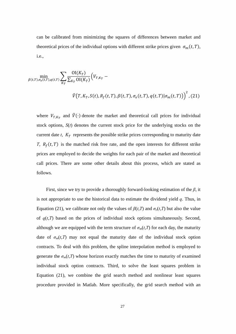
can be calibrated from minimizing the squares of differences between market and

theoretical prices of the individual options with different strike prices given , ,

i.e.,

min, , , , ,

OI∑ OI ,

, , , , , , , , , , | , , 21

where , and · denote the market and theoretical call prices for individual

stock options, S(t) denotes the current stock price for the underlying stocks on the

current date t, represents the possible strike prices corresponding to maturity date

T, , is the matched risk free rate, and the open interests for different strike

prices are employed to decide the weights for each pair of the market and theoretical

call prices. There are some other details about this process, which are stated as

follows.

First, since we try to provide a thoroughly forward-looking estimation of the β, it

is not appropriate to use the historical data to estimate the dividend yield q. Thus, in

Equation (21), we calibrate not only the values of β(t,T) and σe(t,T) but also the value

of q(t,T) based on the prices of individual stock options simultaneously. Second,

although we are equipped with the term structure of σm(t,T) for each day, the maturity

date of σm(t,T) may not equal the maturity date of the individual stock option

contracts. To deal with this problem, the spline interpolation method is employed to

generate the σm(t,T) whose horizon exactly matches the time to maturity of examined

individual stock option contracts. Third, to solve the least squares problem in

Equation (21), we combine the grid search method and nonlinear least squares

procedure provided in Matlab. More specifically, the grid search method with an

28

increment to be 0.01 in a proper range7 is adopted for β, and for each examined value

of the β, the function of lsqnonlin in Matlab is employed to find the optimal values of

σe(t,T) and q(t,T) to minimize the least-squares errors between the market and

theoretical option prices. Finally, among all examined values of β, find the one that

can generate the smallest least-squares errors. Based on the above process, we can

obtain the optimal β(t,T), σe(t,T), and q(t,T) for different maturity date on each date.

IV.3 Empirical Results

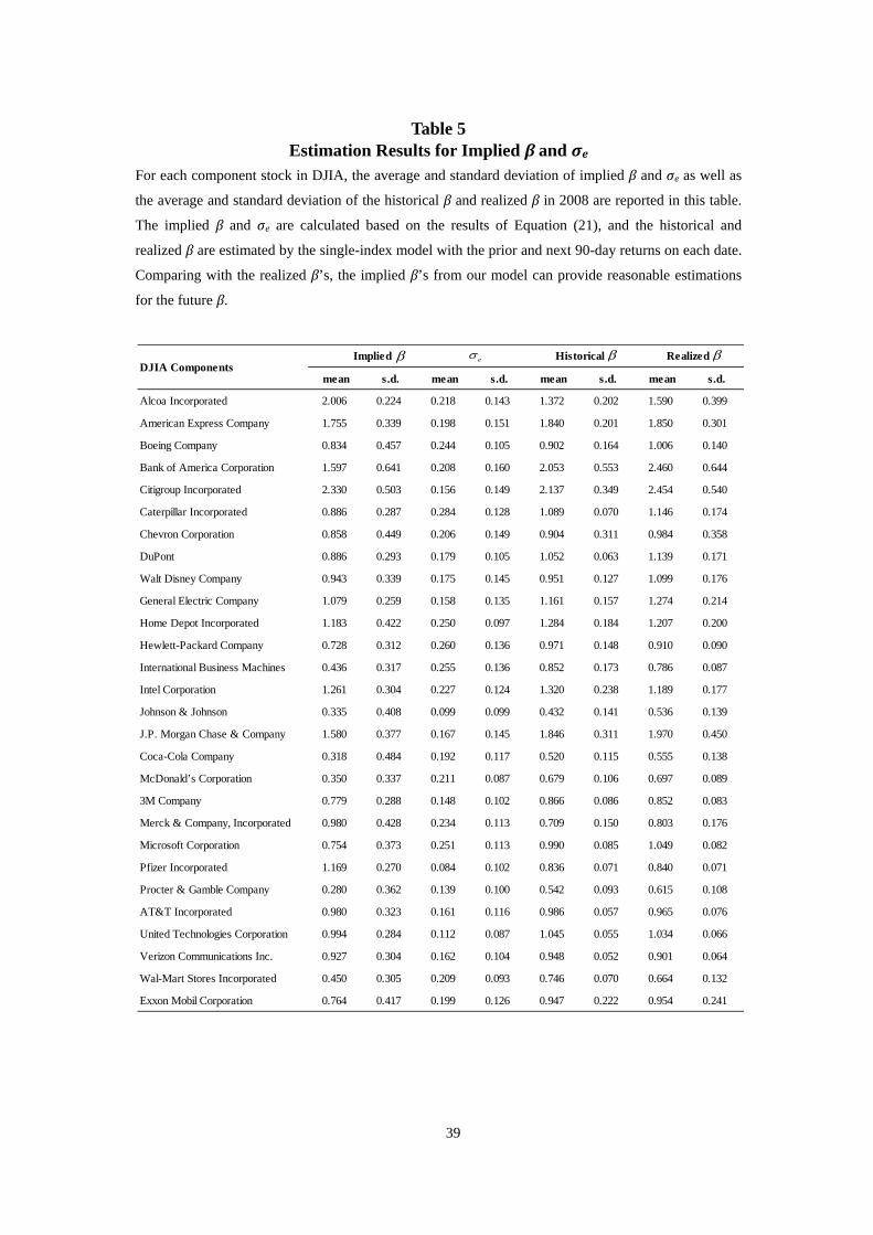
The results of yearly averages and standard deviations of the implied β(t) and σe(t) for

different individual stocks are shown in Table 5. In addition, the historical and

realized β are also reported for comparison. The historical and realized β are

computed based on the single-index model with prior and next 90-day returns,

respectively. It can be observed first that the average values of implied β and eσ for

most stocks are significantly different from 0 by comparing the magnitudes of the

average and the standard deviation. Second, the estimated results suggest that the

option-implied β’s of the individual stocks are in reasonable ranges. The scatter

diagram of realized β’s versus our implied β’s is shown in Figure 4. From the

regression results, the slope coefficient is 0.8876, which is very close to 1, and the

R-squared value is also as high as 0.79. Both evidence that the values of implied β’s

are consistent with the general understanding of the distributions of β’s for the

companies in DJIA. Third, by comparing the implied β from our model with the

historical and realized β, it is obvious to find that the implied β from our model is not

far from the realized β and sometimes is closer to the realized β than the historical β.

7 We derive the average value and standard deviation of the historical betas over prior 90 days to construct a proper range for the grid search method. The average value is adopted to be the central level of the range for β. The upper bound is the result of the average value plus six times the standard deviation, and the lower bound is the result of the average value minus six times the standard deviation. Moreover, if the range of six standard deviations is too narrow (< 0.7) or too wide (> 1.2), 0.7 or 1.2 is used to replace the six standard deviations to generate a proper range for β.

29

However, simply comparing the unconditional averages of the implied and historical

β with the unconditional average of the realized β cannot clearly distinguish the

prediction power between these two estimates. Further studies on this issue are

conducted in the following subsections.

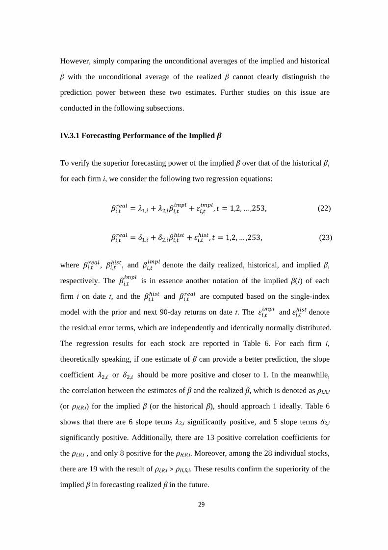
IV.3.1 Forecasting Performance of the Implied β

To verify the superior forecasting power of the implied β over that of the historical β,

for each firm i, we consider the following two regression equations:

, , , , , , 1,2, … ,253, (22)

, , , , , , 1,2, … ,253, (23)

where , , , , and , denote the daily realized, historical, and implied β,

respectively. The , is in essence another notation of the implied β(t) of each

firm i on date t, and the , and , are computed based on the single-index

model with the prior and next 90-day returns on date t. The , and , denote

the residual error terms, which are independently and identically normally distributed.

The regression results for each stock are reported in Table 6. For each firm i,

theoretically speaking, if one estimate of β can provide a better prediction, the slope

coefficient , or , should be more positive and closer to 1. In the meanwhile,

the correlation between the estimates of β and the realized β, which is denoted as ρI,R,i

(or ρH,R,i) for the implied β (or the historical β), should approach 1 ideally. Table 6

shows that there are 6 slope terms λ2,i significantly positive, and 5 slope terms δ2,i

significantly positive. Additionally, there are 13 positive correlation coefficients for

the ρI,R,i , and only 8 positive for the ρH,R,i. Moreover, among the 28 individual stocks,

there are 19 with the result of ρI,R,i > ρH,R,i. These results confirm the superiority of the

implied β in forecasting realized β in the future.

30

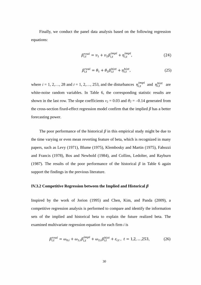
Finally, we conduct the panel data analysis based on the following regression

equations:

, , , , 24

, , , , (25)

where i = 1, 2,…, 28 and t = 1, 2,…, 253, and the disturbances , and , are

white-noise random variables. In Table 6, the corresponding statistic results are

shown in the last row. The slope coefficients v2 = 0.03 and θ2 = –0.14 generated from

the cross-section fixed-effect regression model confirm that the implied β has a better

forecasting power.

The poor performance of the historical β in this empirical study might be due to

the time varying or even mean reverting feature of beta, which is recognized in many

papers, such as Levy (1971), Blume (1975), Klembosky and Martin (1975), Fabozzi

and Francis (1978), Bos and Newbold (1984), and Collins, Ledolter, and Rayburn

(1987). The results of the poor performance of the historical β in Table 6 again

support the findings in the previous literature.

IV.3.2 Competitive Regression between the Implied and Historical β

Inspired by the work of Jorion (1995) and Chen, Kim, and Panda (2009), a

competitive regression analysis is performed to compare and identify the information

sets of the implied and historical beta to explain the future realized beta. The

examined multivariate regression equation for each firm i is

, , , , , , , , 1,2, … ,253, (26)

31

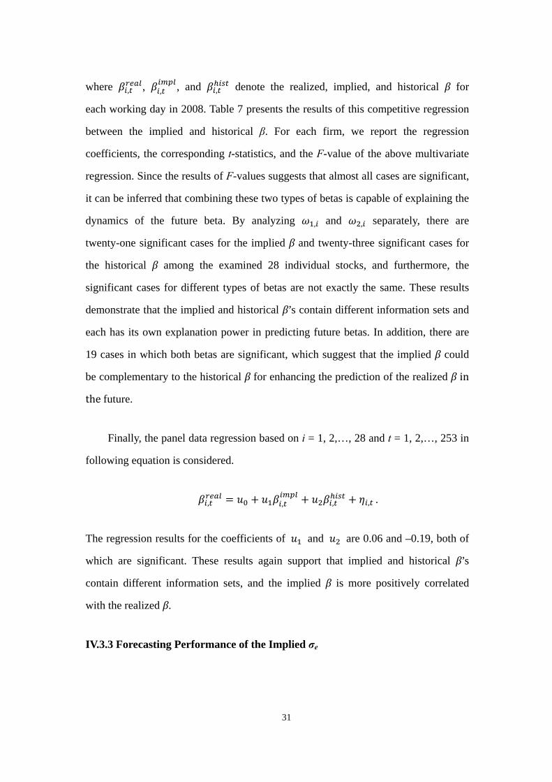
where , , , , and , denote the realized, implied, and historical β for

each working day in 2008. Table 7 presents the results of this competitive regression

between the implied and historical β. For each firm, we report the regression

coefficients, the corresponding t-statistics, and the F-value of the above multivariate

regression. Since the results of F-values suggests that almost all cases are significant,

it can be inferred that combining these two types of betas is capable of explaining the

dynamics of the future beta. By analyzing , and , separately, there are

twenty-one significant cases for the implied β and twenty-three significant cases for

the historical β among the examined 28 individual stocks, and furthermore, the

significant cases for different types of betas are not exactly the same. These results

demonstrate that the implied and historical β’s contain different information sets and

each has its own explanation power in predicting future betas. In addition, there are

19 cases in which both betas are significant, which suggest that the implied β could

be complementary to the historical β for enhancing the prediction of the realized β in

the future.

Finally, the panel data regression based on i = 1, 2,…, 28 and t = 1, 2,…, 253 in

following equation is considered.

, , , , .

The regression results for the coefficients of and are 0.06 and –0.19, both of

which are significant. These results again support that implied and historical β’s

contain different information sets, and the implied β is more positively correlated

with the realized β.

IV.3.3 Forecasting Performance of the Implied σe

32

Traditionally, the systematic risk is the only risk that investors concern. Some recent

literature, however, suggests that idiosyncratic risk might be actually driving a

risk-return relation by examining the cross-sectional relationship between equity

returns and idiosyncratic risk. For example, Lehmann (1990), Merton (1987).

Barberis and Huang (2001) develop asset pricing models and find that future

expected returns are a positive function of idiosyncratic risk. In addition, both the

autoregressive model in Chua, Goh, and Zhang (2006) and the EGARCH models in

Fu (2009) and Spiegel and Wang (2005) find empirically that future expected returns

are positively related to expected idiosyncratic volatilities. In contrast, some other

empirical evidences show different conclusions, such as Ang, Hodrick, Xing, and

Zhang (2006) find a negative cross-sectional relationship between returns and

idiosyncratic risk. In addition, Bali and Cakici (2008) believe that there is no robustly

significant relation between idiosyncratic volatilities and the cross-section of

expected equity returns.

To study this issue, for each firm i, we examine the following regression equation

for realized risk-adjusted excess returns over the implied levels of the idiosyncratic

risk , .

, , , , , , , , 1,2, … ,253, (27)

where , denotes the future 90-day average excess return of the individual stock i,

, denotes the future 90-day average excess market return, , is the realized

beta for the individual stock i , σe,i(t) is the idiosyncratic risk of the individual stocks,

and , is the firm-specific residual. Table 8 shows the regression results of

Equation (27) for each individual stock. The slope coefficients in bold represent the

regression results that are positive and statistically significant. These cases support

the hypothesis that the idiosyncratic risk is able to contribute to future excess return.

33

In contrast, we also find that some of the slope coefficients are negative and

statistically significant. These mixed results are in accordance with that it is still

under debate about whether the idiosyncratic risk can influence future stock returns.

Finally, the panel data regression for all individual stocks and all dates t is also

conducted: , , , , , , for i = 1, 2,…, 28, and t = 1,

2, …, 253. The results of the estimated coefficients, t-statistics, and R-squared are

shown in the last row of Table 8. The slope coefficient is very close to 0, which

inclines to support Bali and Cakici (2008) that the relationship between the

idiosyncratic risk and cross-section of the future excess returns is uncertain and

ambiguous.

V. Conclusion

It is commonly believed that option prices can provide additional information on the

underlying stock prices, particularly about the volatility of the underlying stock prices

in the future. Although option prices are informative about future volatility, there is

little research on using option prices to infer future values of β, which, by definition,

should be determined according to the volatilities of the market index level and the

individual stock prices.

In this paper, a novel method is proposed to estimate the levels of β and the

idiosyncratic risk purely from the prices of market index and individual stock options.

Building on Siegel (1995) and Husmann and Stephen (2007), we develop a

semi-analytical pricing model for individual stock options involving the volatility of

the market index level and the levels of the β and the idiosyncratic risk of the

underlying stock asset through combining the market model and the multivariate

risk-neutral valuation relationship (RNVR) developed in Stapleton and

34

Subrahmanyam (1984) and Câmara (2003). Our analysis demonstrates the superior

ability of this option pricing model to explain the price behavior of individual stock

options found in previous literature, i.e., the higher the levels of the β and the

idiosyncratic risk, the more negatively-sloping implied volatility curves can be

generated, and both these effects diminish with the increase of the time to maturity.

Moreover, we conduct empirical studies to calibrate the β and the idiosyncratic

risk from the prices of index options of DJIA and individual stock options of the

DJIA components, and demonstrate that the values of the β implied from our model

not only provide reasonable estimations for the realized β of firms in DJIA, but also

contain different information sets and provide a better performance versus the

historical β in predicting the realized β for future periods of time. In addition, we also

analyze the relationship between the level of the idiosyncratic risk implied from the

option prices and the future underlying stock returns, and the results support that

there is no robustly significant relation between idiosyncratic risk and the

cross-section of future excess return in the underlying stock.

The option pricing formula incorporating the market model in this paper enables

derivation of forward-looking β of individual stock assets purely based on prices of

stock index and individual stock options. Furthermore, our model has much potential.

For instance, it is possible to apply our estimates of implied β and to test the

validity of the CAPM, and it is possible to incorporate RNVR with more general

option pricing models that take the effects of the skewness and the kurtosis into

account. In addition, one might conduct the analyses for different periods of time and

different markets to further understand the behavior of this forward-looking β

estimation in detail.

35

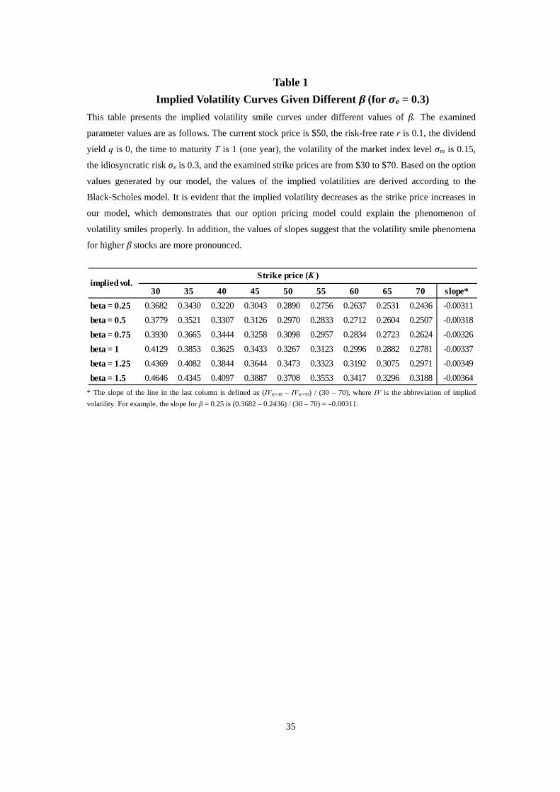
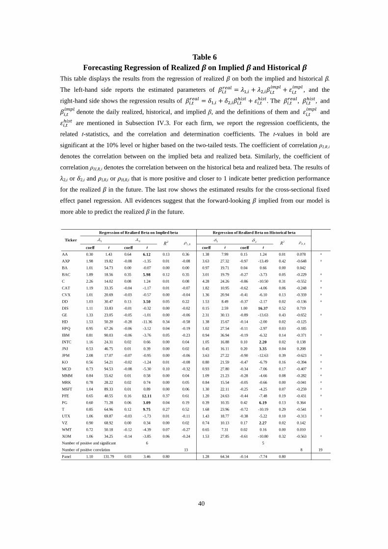
Table 1 Implied Volatility Curves Given Different β (for σe = 0.3)

This table presents the implied volatility smile curves under different values of β. The examined

parameter values are as follows. The current stock price is $50, the risk-free rate r is 0.1, the dividend

yield q is 0, the time to maturity T is 1 (one year), the volatility of the market index level σm is 0.15,

the idiosyncratic risk σe is 0.3, and the examined strike prices are from $30 to $70. Based on the option

values generated by our model, the values of the implied volatilities are derived according to the

Black-Scholes model. It is evident that the implied volatility decreases as the strike price increases in

our model, which demonstrates that our option pricing model could explain the phenomenon of

volatility smiles properly. In addition, the values of slopes suggest that the volatility smile phenomena

for higher β stocks are more pronounced.

* The slope of the line in the last column is defined as (IVK=30 – IVK=70) / (30 – 70), where IV is the abbreviation of implied volatility. For example, the slope for β = 0.25 is (0.3682 – 0.2436) / (30 – 70) = –0.00311.

30 35 40 45 50 55 60 65 70 slope*beta = 0.25 0.3682 0.3430 0.3220 0.3043 0.2890 0.2756 0.2637 0.2531 0.2436 -0.00311beta = 0.5 0.3779 0.3521 0.3307 0.3126 0.2970 0.2833 0.2712 0.2604 0.2507 -0.00318beta = 0.75 0.3930 0.3665 0.3444 0.3258 0.3098 0.2957 0.2834 0.2723 0.2624 -0.00326beta = 1 0.4129 0.3853 0.3625 0.3433 0.3267 0.3123 0.2996 0.2882 0.2781 -0.00337beta = 1.25 0.4369 0.4082 0.3844 0.3644 0.3473 0.3323 0.3192 0.3075 0.2971 -0.00349beta = 1.5 0.4646 0.4345 0.4097 0.3887 0.3708 0.3553 0.3417 0.3296 0.3188 -0.00364

Strike price (K )implied vol.

36

Table 2 Implied Volatility Curves Given Different β (for σe = 0.2 and σe = 0.4)

Based on the numerical example in Table 1, this table reports the implied volatilities smile curves

under different β for a lower and higher levels of the idiosyncratic risk σe. The level of the

idiosyncratic risk σe is 0.2 in Panel A and 0.4 in Panel B. After generating option prices via our model,

the values of the implied volatilities are derived based on the Black-Scholes model. Comparing with

Table 1, it is obvious that the implied volatility smile becomes more pronounced as σe increases in our

model. In other words, the phenomenon of the volatility smile is more pronounced for stocks with

higher idiosyncratic risk.

* The slope of the line in the last column is defined as (IVK=30 – IVK=70) / (30 – 70), where IV means implied volatility. For example, the slope for β = 0.25 in Panel A is (0.2473 – 0.1642) / (30 – 70) = –0.00208.

implied vol. 30 35 40 45 50 55 60 65 70

beta = 0.25 0.2473 0.2305 0.2165 0.2047 0.1945 0.1855 0.1776 0.1706 0.1642 -0.00208beta = 0.5 0.2604 0.2430 0.2286 0.2164 0.2059 0.1968 0.1887 0.1815 0.1751 -0.00213beta = 0.75 0.2800 0.2618 0.2469 0.2342 0.2234 0.2141 0.2059 0.1986 0.1922 -0.00220beta = 1 0.3050 0.2859 0.2702 0.2570 0.2458 0.2361 0.2277 0.2203 0.2138 -0.00228beta = 1.25 0.3345 0.3143 0.2976 0.2838 0.2720 0.2618 0.2530 0.2453 0.2385 -0.00240beta = 1.5 0.3680 0.3462 0.3284 0.3136 0.3010 0.2902 0.2808 0.2726 0.2654 -0.00256


Strike price (K )

Panel B. Implied volatilities for = 0.4

Panel A. Implied volatilities for = 0.2slope*

eσ

eσ

37

Table 3 Implied Volatility Curves Given Different β (for T = 0.25 and T = 2)

This table studies the effect of different time to maturities on the implied volatilities. Under the same

parameter values in Table 1, the volatilities smile become more significant as the time to maturity T

changes from 1 to 0.25. In contrast, the volatilities smile diminishes as the time to maturity T changes

from 1 to 2. Thus, it can be concluded that the volatility smile effect decays with the increase of the

time to maturity, which is consistent with the results of many empirical studies in the literature.

* The slope of the line in the last column is defined as (IVK=30 – IVK=70) / (30 – 70), where IV represents the implied volatility. For example, the slope for β = 0.25 is (0.3815 – 0.2516) / (30 – 70) = –0.00325 as the time to maturity T = 0.25.

implied vol. 30 35 40 45 50 55 60 65 70Panel A. Implied volatilities for T = 0.25


Panel B. Implied volatilities for T = 2


Strike price (K )

slope*

38

Table 4 Descriptive Statistics of Implied Volatilities of Options

This table reports summary statistics for the implied volatilities of the call option contracts used in this

paper. We collect index call options for DJIA as well as the call option contracts for its component

firms in 2008. Option prices are collected from OptionMetrics, but only 28 component stocks are

examined due to the availability problem of the option prices of General Motors (GM) and American

International Group Inc. (AIG), which are removed from the portfolio of the DJIA in June of 2009 and

September of 2008, respectively. In addition, the American option prices of individual stock options

are converted to the counterpart European option prices in a proper procedure introduced in Subsection

IV.1. Implied volatilities are calculated through the Black-Scholes model, and we report the number of

quotations and the means and standard deviations of the implied volatilities for individual stock call

options and market index call options.

DJIA Components # of Qutoes Mean s.d.

Alcoa Incorporated 6144 0.54 0.18

American Express Company 8988 0.61 0.31

Boeing Company 7773 0.43 0.18

Bank of American 8866 0.68 0.35

Citigroup Incorporated 6426 0.71 0.33

Caterpillar Incorporated 8945 0.45 0.19

Chevron Corporation 8133 0.43 0.25

DuPont 5846 0.38 0.16

Walt Disney Company 5084 0.39 0.17

General Electric Company 9573 0.45 0.27

Home Depot Incorporated 5989 0.51 0.19

Hewlett-Packard Company 7832 0.41 0.16

International Business Machines 8715 0.37 0.16

Intel Corporation 6065 0.45 0.14

Johnson & Johnson 3873 0.28 0.14

J.P. Morgan Chase & Company 8874 0.63 0.30

Coca-Cola Company 7220 0.31 0.14

McDonald’s Corporation 7820 0.35 0.14

3M Company 6249 0.35 0.16

Merck & Company, Incorporated 6561 0.40 0.13

Microsoft Corporation 7645 0.39 0.15

Pfizer Incorporated 2978 0.40 0.18

Procter & Gamble Company 6497 0.30 0.16

AT&T Incorporated 6324 0.40 0.16

United Technologies Corporation 7020 0.40 0.18

Verizon Communications Inc. 4489 0.38 0.17

Wal-Mart Stores Incorporated 7710 0.37 0.18

Exxon Mobil Corporation 7336 0.43 0.31

DJX index option 102842 0.30 0.15

39

Table 5 Estimation Results for Implied β and σe

For each component stock in DJIA, the average and standard deviation of implied β and σe as well as

the average and standard deviation of the historical β and realized β in 2008 are reported in this table.

The implied β and σe are calculated based on the results of Equation (21), and the historical and

realized β are estimated by the single-index model with the prior and next 90-day returns on each date.

Comparing with the realized β’s, the implied β’s from our model can provide reasonable estimations

for the future β.

mean s.d. mean s.d. mean s.d. mean s.d.

Alcoa Incorporated 2.006 0.224 0.218 0.143 1.372 0.202 1.590 0.399

American Express Company 1.755 0.339 0.198 0.151 1.840 0.201 1.850 0.301

Boeing Company 0.834 0.457 0.244 0.105 0.902 0.164 1.006 0.140

Bank of America Corporation 1.597 0.641 0.208 0.160 2.053 0.553 2.460 0.644

Citigroup Incorporated 2.330 0.503 0.156 0.149 2.137 0.349 2.454 0.540

Caterpillar Incorporated 0.886 0.287 0.284 0.128 1.089 0.070 1.146 0.174

Chevron Corporation 0.858 0.449 0.206 0.149 0.904 0.311 0.984 0.358

DuPont 0.886 0.293 0.179 0.105 1.052 0.063 1.139 0.171

Walt Disney Company 0.943 0.339 0.175 0.145 0.951 0.127 1.099 0.176

General Electric Company 1.079 0.259 0.158 0.135 1.161 0.157 1.274 0.214

Home Depot Incorporated 1.183 0.422 0.250 0.097 1.284 0.184 1.207 0.200

Hewlett-Packard Company 0.728 0.312 0.260 0.136 0.971 0.148 0.910 0.090

International Business Machines 0.436 0.317 0.255 0.136 0.852 0.173 0.786 0.087

Intel Corporation 1.261 0.304 0.227 0.124 1.320 0.238 1.189 0.177

Johnson & Johnson 0.335 0.408 0.099 0.099 0.432 0.141 0.536 0.139

J.P. Morgan Chase & Company 1.580 0.377 0.167 0.145 1.846 0.311 1.970 0.450

Coca-Cola Company 0.318 0.484 0.192 0.117 0.520 0.115 0.555 0.138

McDonald’s Corporation 0.350 0.337 0.211 0.087 0.679 0.106 0.697 0.089

3M Company 0.779 0.288 0.148 0.102 0.866 0.086 0.852 0.083

Merck & Company, Incorporated 0.980 0.428 0.234 0.113 0.709 0.150 0.803 0.176

Microsoft Corporation 0.754 0.373 0.251 0.113 0.990 0.085 1.049 0.082

Pfizer Incorporated 1.169 0.270 0.084 0.102 0.836 0.071 0.840 0.071

Procter & Gamble Company 0.280 0.362 0.139 0.100 0.542 0.093 0.615 0.108

AT&T Incorporated 0.980 0.323 0.161 0.116 0.986 0.057 0.965 0.076

United Technologies Corporation 0.994 0.284 0.112 0.087 1.045 0.055 1.034 0.066

Verizon Communications Inc. 0.927 0.304 0.162 0.104 0.948 0.052 0.901 0.064

Wal-Mart Stores Incorporated 0.450 0.305 0.209 0.093 0.746 0.070 0.664 0.132

Exxon Mobil Corporation 0.764 0.417 0.199 0.126 0.947 0.222 0.954 0.241

DJIA Components Implied Historical Realized β eσ β β

40

Table 6 Forecasting Regression of Realized β on Implied β and Historical β

This table displays the results from the regression of realized β on both the implied and historical β.

The left-hand side reports the estimated parameters of , , , , , , and the

right-hand side shows the regression results of , , , , , . The , , , , and

, denote the daily realized, historical, and implied β, and the definitions of them and , and

, are mentioned in Subsection IV.3. For each firm, we report the regression coefficients, the

related t-statistics, and the correlation and determination coefficients. The t-values in bold are

significant at the 10% level or higher based on the two-tailed tests. The coefficient of correlation ρI,R,i

denotes the correlation between on the implied beta and realized beta. Similarly, the coefficient of

correlation ρH,R,i denotes the correlation between on the historical beta and realized beta. The results of

λ2,i or δ2,i and ρI,R,i or ρH,R,i that is more positive and closer to 1 indicate better prediction performance

for the realized β in the future. The last row shows the estimated results for the cross-sectional fixed

effect panel regression. All evidences suggest that the forward-looking β implied from our model is

more able to predict the realized β in the future.

coeff t coeff t coeff t coeff t

AA 0.30 1.43 0.64 6.12 0.13 0.36 1.38 7.99 0.15 1.24 0.01 0.078 *

AXP 1.98 19.82 -0.08 -1.35 0.01 -0.08 3.63 27.32 -0.97 -13.49 0.42 -0.648 *

BA 1.01 54.73 0.00 -0.07 0.00 0.00 0.97 19.71 0.04 0.66 0.00 0.042

BAC 1.89 18.56 0.35 5.98 0.12 0.35 3.01 19.79 -0.27 -3.73 0.05 -0.229 *

C 2.26 14.02 0.08 1.24 0.01 0.08 4.28 24.26 -0.86 -10.50 0.31 -0.552 *

CAT 1.19 33.35 -0.04 -1.17 0.01 -0.07 1.82 10.95 -0.62 -4.06 0.06 -0.248 *

CVX 1.01 20.69 -0.03 -0.57 0.00 -0.04 1.36 20.94 -0.41 -6.10 0.13 -0.359 *

DD 1.03 30.47 0.13 3.50 0.05 0.22 1.53 8.49 -0.37 -2.17 0.02 -0.136 *

DIS 1.11 33.83 -0.01 -0.32 0.00 -0.02 0.15 2.59 1.00 16.37 0.52 0.719

GE 1.33 23.05 -0.05 -1.01 0.00 -0.06 2.31 30.13 -0.89 -13.63 0.43 -0.652 *

HD 1.53 50.20 -0.28 -11.36 0.34 -0.58 1.38 15.67 -0.14 -2.00 0.02 -0.125

HPQ 0.95 67.26 -0.06 -3.12 0.04 -0.19 1.02 27.54 -0.11 -2.97 0.03 -0.185

IBM 0.81 90.03 -0.06 -3.76 0.05 -0.23 0.94 36.94 -0.19 -6.32 0.14 -0.371 *

INTC 1.16 24.31 0.02 0.66 0.00 0.04 1.05 16.88 0.10 2.20 0.02 0.138

JNJ 0.53 46.75 0.01 0.39 0.00 0.02 0.45 16.11 0.20 3.35 0.04 0.208

JPM 2.08 17.07 -0.07 -0.95 0.00 -0.06 3.63 27.22 -0.90 -12.63 0.39 -0.623 *

KO 0.56 54.21 -0.02 -1.24 0.01 -0.08 0.80 21.59 -0.47 -6.79 0.16 -0.394 *

MCD 0.73 94.53 -0.08 -5.30 0.10 -0.32 0.93 27.80 -0.34 -7.06 0.17 -0.407 *

MMM 0.84 55.62 0.01 0.58 0.00 0.04 1.09 21.23 -0.28 -4.66 0.08 -0.282 *

MRK 0.78 28.22 0.02 0.74 0.00 0.05 0.84 15.54 -0.05 -0.66 0.00 -0.041 *

MSFT 1.04 89.33 0.01 0.89 0.00 0.06 1.30 22.11 -0.25 -4.25 0.07 -0.259 *

PFE 0.65 40.55 0.16 12.11 0.37 0.61 1.20 24.63 -0.44 -7.48 0.19 -0.431 *

PG 0.60 71.28 0.06 3.09 0.04 0.19 0.39 10.35 0.42 6.19 0.13 0.364

T 0.85 64.96 0.12 9.75 0.27 0.52 1.68 23.96 -0.72 -10.19 0.29 -0.541 *

UTX 1.06 69.87 -0.03 -1.73 0.01 -0.11 1.43 18.77 -0.38 -5.22 0.10 -0.313 *

VZ 0.90 68.92 0.00 0.34 0.00 0.02 0.74 10.13 0.17 2.27 0.02 0.142

WMT 0.72 50.18 -0.12 -4.39 0.07 -0.27 0.65 7.31 0.02 0.16 0.00 0.010

XOM 1.06 34.25 -0.14 -3.85 0.06 -0.24 1.53 27.85 -0.61 -10.80 0.32 -0.563 *

Number of positive and significant 6 5

Number of positive correlation 13 8 19

Panel 1.10 131.79 0.03 3.46 0.80 1.28 64.34 -0.14 -7.74 0.80

Ticker

Regression of Realized Beta on Implied beta Regression of Realized Beta on Historical beta

2R 2R ,H Rρ,I Rρ1λ 2λ 2δ1δ

41

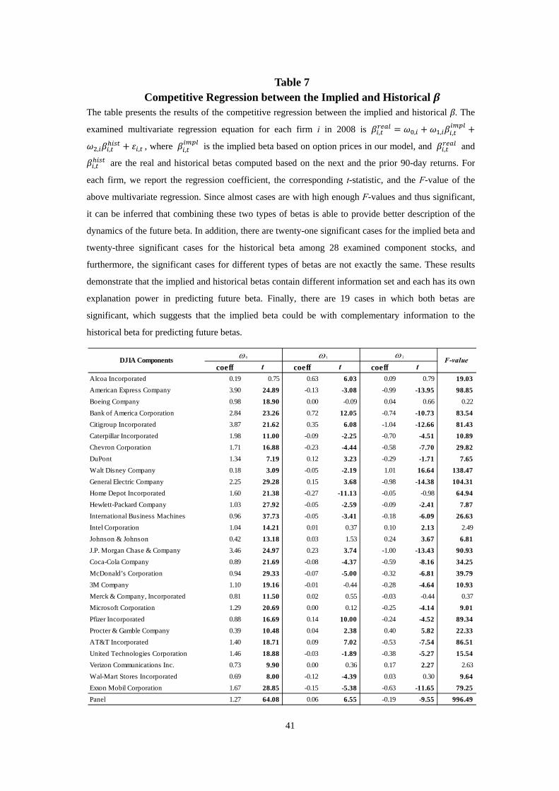
Table 7 Competitive Regression between the Implied and Historical β

The table presents the results of the competitive regression between the implied and historical β. The

examined multivariate regression equation for each firm i in 2008 is , , , ,

, , , , where , is the implied beta based on option prices in our model, and , and

, are the real and historical betas computed based on the next and the prior 90-day returns. For

each firm, we report the regression coefficient, the corresponding t-statistic, and the F-value of the

above multivariate regression. Since almost cases are with high enough F-values and thus significant,

it can be inferred that combining these two types of betas is able to provide better description of the

dynamics of the future beta. In addition, there are twenty-one significant cases for the implied beta and

twenty-three significant cases for the historical beta among 28 examined component stocks, and

furthermore, the significant cases for different types of betas are not exactly the same. These results

demonstrate that the implied and historical betas contain different information set and each has its own

explanation power in predicting future beta. Finally, there are 19 cases in which both betas are

significant, which suggests that the implied beta could be with complementary information to the

historical beta for predicting future betas.

coeff t coeff t coeff tAlcoa Incorporated 0.19 0.75 0.63 6.03 0.09 0.79 19.03American Express Company 3.90 24.89 -0.13 -3.08 -0.99 -13.95 98.85Boeing Company 0.98 18.90 0.00 -0.09 0.04 0.66 0.22Bank of America Corporation 2.84 23.26 0.72 12.05 -0.74 -10.73 83.54Citigroup Incorporated 3.87 21.62 0.35 6.08 -1.04 -12.66 81.43Caterpillar Incorporated 1.98 11.00 -0.09 -2.25 -0.70 -4.51 10.89Chevron Corporation 1.71 16.88 -0.23 -4.44 -0.58 -7.70 29.82DuPont 1.34 7.19 0.12 3.23 -0.29 -1.71 7.65Walt Disney Company 0.18 3.09 -0.05 -2.19 1.01 16.64 138.47General Electric Company 2.25 29.28 0.15 3.68 -0.98 -14.38 104.31Home Depot Incorporated 1.60 21.38 -0.27 -11.13 -0.05 -0.98 64.94Hewlett-Packard Company 1.03 27.92 -0.05 -2.59 -0.09 -2.41 7.87International Business Machines 0.96 37.73 -0.05 -3.41 -0.18 -6.09 26.63Intel Corporation 1.04 14.21 0.01 0.37 0.10 2.13 2.49Johnson & Johnson 0.42 13.18 0.03 1.53 0.24 3.67 6.81J.P. Morgan Chase & Company 3.46 24.97 0.23 3.74 -1.00 -13.43 90.93Coca-Cola Company 0.89 21.69 -0.08 -4.37 -0.59 -8.16 34.25McDonald’s Corporation 0.94 29.33 -0.07 -5.00 -0.32 -6.81 39.793M Company 1.10 19.16 -0.01 -0.44 -0.28 -4.64 10.93Merck & Company, Incorporated 0.81 11.50 0.02 0.55 -0.03 -0.44 0.37Microsoft Corporation 1.29 20.69 0.00 0.12 -0.25 -4.14 9.01Pfizer Incorporated 0.88 16.69 0.14 10.00 -0.24 -4.52 89.34Procter & Gamble Company 0.39 10.48 0.04 2.38 0.40 5.82 22.33AT&T Incorporated 1.40 18.71 0.09 7.02 -0.53 -7.54 86.51United Technologies Corporation 1.46 18.88 -0.03 -1.89 -0.38 -5.27 15.54Verizon Communications Inc. 0.73 9.90 0.00 0.36 0.17 2.27 2.63Wal-Mart Stores Incorporated 0.69 8.00 -0.12 -4.39 0.03 0.30 9.64Exxon Mobil Corporation 1.67 28.85 -0.15 -5.38 -0.63 -11.65 79.25Panel 1.27 64.08 0.06 6.55 -0.19 -9.55 996.49

DJIA Components F-value1ω0ω 2ω

42

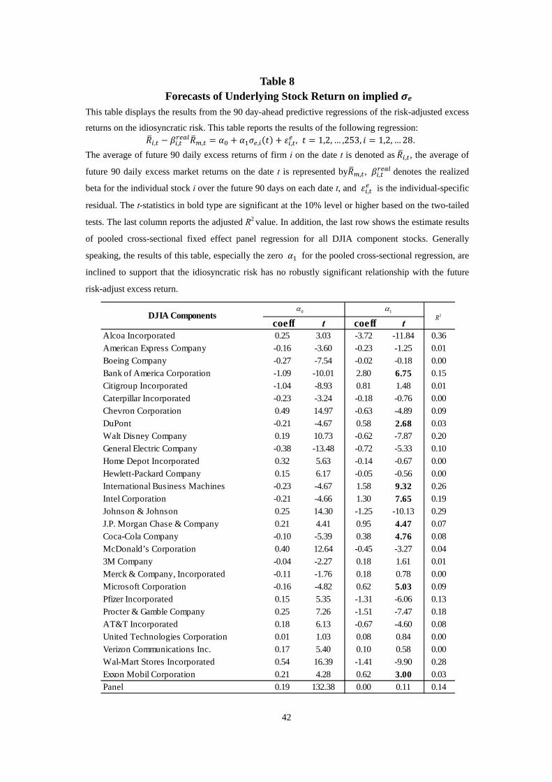
Table 8 Forecasts of Underlying Stock Return on implied σe

This table displays the results from the 90 day-ahead predictive regressions of the risk-adjusted excess

returns on the idiosyncratic risk. This table reports the results of the following regression: , , , , , , 1,2, … ,253, 1,2, … 28.

The average of future 90 daily excess returns of firm i on the date t is denoted as , , the average of

future 90 daily excess market returns on the date t is represented by , , , denotes the realized

beta for the individual stock i over the future 90 days on each date t, and , is the individual-specific

residual. The t-statistics in bold type are significant at the 10% level or higher based on the two-tailed

tests. The last column reports the adjusted R2 value. In addition, the last row shows the estimate results

of pooled cross-sectional fixed effect panel regression for all DJIA component stocks. Generally

speaking, the results of this table, especially the zero for the pooled cross-sectional regression, are

inclined to support that the idiosyncratic risk has no robustly significant relationship with the future

risk-adjust excess return.

coeff t coeff tAlcoa Incorporated 0.25 3.03 -3.72 -11.84 0.36American Express Company -0.16 -3.60 -0.23 -1.25 0.01Boeing Company -0.27 -7.54 -0.02 -0.18 0.00Bank of America Corporation -1.09 -10.01 2.80 6.75 0.15Citigroup Incorporated -1.04 -8.93 0.81 1.48 0.01Caterpillar Incorporated -0.23 -3.24 -0.18 -0.76 0.00Chevron Corporation 0.49 14.97 -0.63 -4.89 0.09DuPont -0.21 -4.67 0.58 2.68 0.03Walt Disney Company 0.19 10.73 -0.62 -7.87 0.20General Electric Company -0.38 -13.48 -0.72 -5.33 0.10Home Depot Incorporated 0.32 5.63 -0.14 -0.67 0.00Hewlett-Packard Company 0.15 6.17 -0.05 -0.56 0.00International Business Machines -0.23 -4.67 1.58 9.32 0.26Intel Corporation -0.21 -4.66 1.30 7.65 0.19Johnson & Johnson 0.25 14.30 -1.25 -10.13 0.29J.P. Morgan Chase & Company 0.21 4.41 0.95 4.47 0.07Coca-Cola Company -0.10 -5.39 0.38 4.76 0.08McDonald’s Corporation 0.40 12.64 -0.45 -3.27 0.043M Company -0.04 -2.27 0.18 1.61 0.01Merck & Company, Incorporated -0.11 -1.76 0.18 0.78 0.00Microsoft Corporation -0.16 -4.82 0.62 5.03 0.09Pfizer Incorporated 0.15 5.35 -1.31 -6.06 0.13Procter & Gamble Company 0.25 7.26 -1.51 -7.47 0.18AT&T Incorporated 0.18 6.13 -0.67 -4.60 0.08United Technologies Corporation 0.01 1.03 0.08 0.84 0.00Verizon Communications Inc. 0.17 5.40 0.10 0.58 0.00Wal-Mart Stores Incorporated 0.54 16.39 -1.41 -9.90 0.28Exxon Mobil Corporation 0.21 4.28 0.62 3.00 0.03Panel 0.19 132.38 0.00 0.11 0.14

DJIA Components 2R1α0α

43

0.1500

0.2000

0.2500

0.3000

0.3500

0.4000

0.4500

0.5000

0.5500

0.6000

30 35 40 45 50 55 60 65 70

beta = 0.25

beta = 0.5

beta = 0.75

beta = 1

beta = 1.25

beta = 1.5

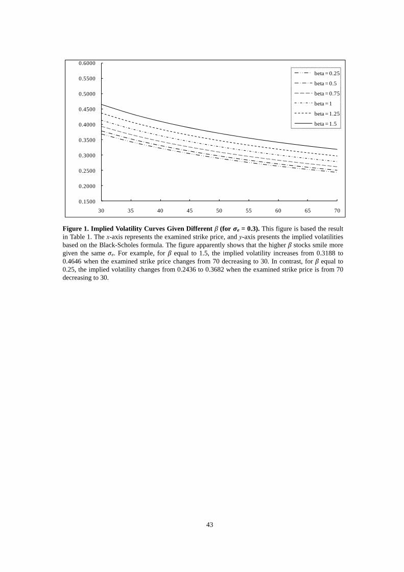
Figure 1. Implied Volatility Curves Given Different β (for σe = 0.3). This figure is based the result in Table 1. The x-axis represents the examined strike price, and y-axis presents the implied volatilities based on the Black-Scholes formula. The figure apparently shows that the higher β stocks smile more given the same σe. For example, for β equal to 1.5, the implied volatility increases from 0.3188 to 0.4646 when the examined strike price changes from 70 decreasing to 30. In contrast, for β equal to 0.25, the implied volatility changes from 0.2436 to 0.3682 when the examined strike price is from 70 decreasing to 30.

44

0.1500

0.2000

0.2500

0.3000

0.3500

0.4000

0.4500

0.5000

0.5500

0.6000

30 35 40 45 50 55 60 65 70

beta = 0.25beta = 0.5beta = 0.75beta = 1beta = 1.25beta = 1.5

Figure 2. Implied Volatility Curves Given Different β (for σe = 0.2 and σe = 0.4). This figure is based on the results in Table 2. The x-axis represents the examined strike price, and the implied volatility based on the Black-Shoes model is on the y-axis. This figure demonstrates that the volatility smile phenomenon for higher idiosyncratic risk stocks is more pronounced. For example, when β equals 1.5, the slope of the volatilities smile curve (defined as (IVK=30 – IVK=70) / (30 – 70) in Table 2), is –0.00256 for σe = 0.2 and –0.00470 for σe = 0.4.

0.1500

0.2000

0.2500

0.3000

0.3500

0.4000

0.4500

0.5000

0.5500

0.6000

30 35 40 45 50 55 60 65 70


0.2eσ = 0.4eσ =

45

Figure 3 Implied Volatility Curves Given Different β (for T = 0.25 and T = 2) The above diagrams report the relationship between volatility smile and the time to maturity. The left-side diagram presents the volatility smile as the time to maturity T = 0.25, and the right-side diagram presents the volatility smile as the time to maturity T = 2. Comparing these two figures, it is able to conclude that the volatilities smile phenomenon decays as the time to maturity T increases.

0.1500

0.2000

0.2500

0.3000

0.3500

0.4000

0.4500

0.5000

0.5500

0.6000

30 35 40 45 50 55 60 65 70


0.1500

0.2000

0.2500

0.3000

0.3500

0.4000

0.4500

0.5000

0.5500

0.6000

30 35 40 45 50 55 60 65 70


0.25T = 2T =

Figudiagregrvalucom

ure 4 The Sgram of the avression resultsue is also as h

mponent stocks

catter Diagrverage realizeds are also repohigh as 0.79. Bs of DJIA belo

am for Reald β and implieorted. The slopBoth evidenceonging to vari

46

lized β versued β of the compe coefficient e that our modious industries

us Implied β.mponent stockis 0.8876, wh

del can generas.

. This figure ks in DJIA. Inhich is close toate reasonable

shows the scn addition, theo 1. The R-sque levels of β fo

catter e least uared or the

47

Appendix I

Before deriving the option pricing formula based on the market model, we first

demonstrate some results of the integrals based upon the normal distributions. The

definition of the probability density function of a normal distributed random variable

~ , is

√

· , (A.1)

where μx and σx are the mean and the standard deviation of , respectively. The following

three results of integrals are useful in the following derivation of the option price

formulae.

Result 1. The integral of :

, (A.2)

where N(z*) is the cumulative distribution function for the standard normal distribution

from –∞ to z*, that is, 2 ⁄ · ⁄ .

Result 2. The integral of the product of :

· · · . (A.3)

The proof for Equation (A.3) is as follows. Define z = (x – μx) / σx, and we can obtain

· · ·√ √

48

√·

· · ,

where 2 · , which is the probability density function of the standard

normal distribution.

Result 3. The integral of the product of :

· . (A.4)

The proof for the above formula is as follows.

·√

·√

·

√·

√·

√

·

√

·

√ by defining ⁄

· .

49

Appendix II

According to Equation (14), the current option value can be expressed as

max 1 , 0 · ,

where and are the risk-neutral standard normal probability density

functions for ~ ln , and ~ 0, , and √ √

·

exp ln and √ √

·

exp 0 .

Case 1. For β > 0, the option value in Equation (15) is as follows.

1

1 ,

(A.5)

where ln ln , which implies and .

For the first integral in Equation (A.5),

50

1 ·

8

·

·

· –

√√ ·

√

· √ · , (A.6)

where √

, and the last equation is derived based on the definitions of

and .

As to the second integral in Equation (A.5),

1 ·

1 ·

·

1

–

√

8 Suppose the value of Ze is given. The result of the integral 1 is 1 ·

1

1 ·ln

2

2

√1

·ln

2

2

√ .

Therefore, when c ∞, the result for 1 · will

converge to 1 · 1 · 1 .

by (A.2) & (A.3)

by (A.2) & (A.4)

by (A.2) & (A.4)

51

· · ln ln 2

√

1 ·

· · , (A.7)

where √

and √

√ . As a

result, the sum of Equations (A.6) and (A.7) is the result for the integral in Equation (A.5).

Case 2. For β = 0, the option value in Equation (17) is as follows.

·

· ·

·

√√ ·

√.

· √ · , (A.8)

where √

.

Case 3. For β < 0, the option price formula is as follows.

1

1 ·

by (A.2) & (A.3)

52

· ·

1

√

·

√

1 ·

· · . (A.9)

by (A.2) & (A.4)

53

Appendix III

In Equation (7), if β = 1 and the normally distributed random variable re is fixed at zero,

the payoff function becomes the one for a market index call option if S0 represents the

market index level today. If σe = 0, we can derive 0 in probability 1.

Since Ze is fixed at zero, the integral over Ze can be dropped. Furthermore, due to the fact

that 1 is larger than zero, we can obtain ∞ 0

1 and thus only the second term in Equation (15) needed to be considered.

· ·

· ·

· · · ·

√

· · ·√

· ·√

· ·√

.

By substituting and with and , the above equation can be rewritten

to be identical to the Black-Scholes formula for the market index call options:

·√

· ·√

.

by (A.2) & (A.4)

54

REFERENCES

Adrian, Tobias, and Francesco Franzoni, 2009, Time-Varying Factor Loadings, Expected Returns, and the Conditional CAPM, Journal of Empirical Finance 16, 537–556.

Ang, Andrew, Robert J. Hodrick, Yuhang Xing, and Xiaoyan Zhang, 2006, The Cross-Section of Volatility and Expected Returns, Journal of Finance 61, 259–299.

Backus, David, Silverio Foresi, and Liuren Wu, 2004, Accounting for Biases in Black-Scholes, working paper, Stern School of Business, New York University

Baesel, Jerome B., 1974, On the Assessment of Risk: Some Further Consideration, Journal of Finance 27, 1491–1494.

Bakshi, Gurdip, Nikunj Kapadia, and Dilip Madan, 2003, Stock Return Characteristics, Skew Laws, and the Differential Pricing of Individual Equity Options. Review of Financial Studies 16, 101–143.

Bali, Turan G., and Nusret Cakici, 2008, Idiosyncratic Volatility and the Cross Section of Expected Returns, Journal of Financial and Quantitative Analysis 43, 29–58.

Barberis, Nocolas, and Ming Huang, 2001, Mental Accounting, Loss Aversion, and Individual Stock Returns, Journal of Finance 56, 1247–1292.

Bates, David S., 1998, Post-’87 Crash Fears in the S&P500 Futures Option Market, Journal of Econometrics 46, 181–238.

Black, Fisher, and Myron Scholes, 1973, The Pricing of Options and Corporate Liabilities, Journal of Political Economy 81, 637–659.

Blume, Marshall E., 1971, On the Assessment of Risk, Journal of Finance 26, 1–10. Blume, Marshall E., 1975, Betas and Their Regression Tendencies, Journal of Finance 30,

785–795. Bos, T., and P. Newbold, 1984, An Empirical Investigation of the Possibility of Stochastic

Systematic Risk in the Market Model, Journal of Business 57, 35–41. Brennan, Michael J., 1979, The Pricing of Contingent Claims in Discrete Time Models,

Journal of Finance 34, 53–68. Buraschi, Andrea, and Jens Jackwerth, 2001, The Price of a Smile: Hedging and Spanning

in Option Markets, Review of Financial Studies 14, 495–527. Câmara, António, 2003, A Generalization of the Brennan-Rubinstein Approach for the

Pricing of Derivatives, Journal of Finance 58, 805–819. Câmara, António, 2005, Option prices Sustained by Risk-Preferences, Journal of Business

78, 1683–1708. Chang, Bo-Young, Peter Christoffersen, Kris Jacobs, and Gregory Vainberg, 2010,

Option-Implied Measures of Equity Risk, working paper. Chen, Ren-Raw, Doncheol Kim, and Durga Panda, 2009, On the Ex-Ante Cross-Sectional

Relation Between Risk and Return Using Option-Implied Information, working paper.

55

Chua, Choong Tze, Jeremy Goh, and Zhe Zhang, 2006, Idiosyncratic Volatility Matters for the Cross-Section of Returns-in More Ways than One!, working paper.

Collins, Daniel W., Johannes Ledolter, and Judy Rayburn, 1987, Some Further Evidence on the Stochastic Properties of Systematic Risk, Journal of Business 60, 425–449.

Dennis, Patrick, and Stewart Mayhew, 2002, Risk-Neutral Skewness: Evidence from Stock Options, Journal of Financial and Quantitative Analysis 37, 471–493.

Duan, Jin-Chuan, and Jason Wei, 2009, Systematic Risk and the Price Structure of Individual Equity Options, Review of Financial Studies 22, 1981–2006.

Duque, João L. C, Patrícia Teixeira Lopes, 2003, Maturity and Volatility Effects on Smiles or Dying Smiling, Portuguese Economic Journal 2, 173–193.

Fabozzi, Frank J., and Jack Clark Francis, 1978, Beta as A Random Coefficient, Journal of Financial and Quantitative Analysis 13, 101–116.

Faff, Robert W., John H.H. Lee, and Tim R.L. Fry, 1992, Time Stationarity of Systematic Risk: Some Australian Evidence, Journal of Business Finance and Accounting 19, 253–270.

Fama, Eugene F., and Kenneth R. French, 1992, The Cross-Section of Expected Stock Returns, Journal of Finance 47, 427–465.

Ferson, Wayne E., and Campbell R. Harvey, 1999, Conditioning Variables and the Cross Section of Stock Returns, Journal of Finance 54, 1325–1360.

Ferson, Wayne E., Shmuel Kandel, and Robert F. Stambaugh, 1987, Tests of Asset Pricing with Time-Varying Expected Risk Premiums and Market Betas, Journal of Finance 42, 201–220.

Fu, Fangjian, 2009, Idiosyncratic Risk and the Cross-Section of Expected Stock Returns, Journal of Financial Economics 91, 24–37.

Fraser, Patricia, Foort Hamelink, Martin Hoesli, and Bryan Macgregor, 2004, Time-Varying Betas and the Cross-Sectional Return-Risk Relation: Evidence from the UK, European Journal of Finance 10, 255–276.

French, Dan W., John C. Groth, and James W. Kolari, 1983, Current Investor Expectations and Better Betas, Journal of Portfolio Management 10, 12–17.

Husmann, Sven, and Andreas Stephan, 2007, On Estimating an Asset’s Implicit Beta, Journal of Futures Markets 27, 961–979.

Jackwerth, Jens Carsten, 2000, Recovering Risk Aversion from Option Prices and Realized Returns, Review of Financial Studies 13, 433–451.

Jagannathan, Ravi, and Zhenyu Wang, 1996, The Conditional CAPM and the Cross-Section of Expected Returns, Journal of Finance 51, 3–53.

Jarrow, Robbert A, and Dilip B. Madan, 1997, Is Mean-Variance Analysis Vacuous: Or was Beta Still Born?, European Finance Review 1, 15–30.

Jensen, Michael C., 1968, The Performance of Mutual Funds in the Period 1945-64, Journal of Finance 23, 389–416.

56

Jorion, Philippe, 1995, Predicting Volatility in the Foreign Exchange Market, Journal of Finance 50, 507–528.

Klemkosky, Robert C., and John D. Martin, 1975, The Adjustment of Beta Forecasts, Journal of Finance 30, 1123–1128.

Lehmann, Bruce N., 1990, Residual Risk Revisited, Journal of Econometrics 45, 71–97. Lintner, John, 1965, The Valuation of Risk Assets and the Selection of Risky Investments

in Stock Portfolios and Capital Budgets, Review of Economics and Statistics 47, 13–37.

Levy, Robert A., 1971, On the Short-term Stationarity of Beta Coefficients, Financial Analysis Journal 27, 55–62.

Macbeth, James D., Larry J. Merville, 1979, An Empirical Examination of the Black-Scholes Call Option Pricing Model, Journal of Finance 34, 1173–1186.

Margrabe, William, 1978, The Value of an Option to Exchange One Asset for Another, Journal of Finance 18, 177–186.

Merton, Robert C., 1987, A Simple Model of Capital Market Equilibrium with Incomplete Information, Journal of Finance 42, 483–510.

Park, Kwang Woo, 2004, Time-Series Analysis of Return and Beta in U.S., Journal of Academy of Business and Economics 3, 43–54.

Roenfeldt, Rodney L., Gary L. Griepentrog, and Christopher C. Pflaum, 1978, Further Evidence on the Stationarity of Beta Coefficients, Journal of Financial and Quantitative Analysis 13, 117–121.

Roll, Richard, 1977, A Critique of the Asset Pricing Theory's Tests Part I: On Past and Potential Testability of the Theory, Journal of Financial Economics 4, 129–176.

Rubinstein, Mark, 1976, The Valuation of Uncertain Income Streams and the Pricing of Options, Bell Journal of Economics 7, 407–425.

Rubinstein, Mark, 1985, Nonparametric Tests of Alternative Option pricing Models Using all Reported Trades and Quotes on the 30 Most Active CBOE Option Classes from August 23, 1976 Through August 31,1978, Journal of Finance 40, 455–480.

Rubinstein, Mark, 1994, Implied Binomial Trees, Journal of Finance 49, 771–818. Sharpe, William F., 1964, Capital Asset Prices: A Theory of Market Equilibrium Under

Conditions of Risk, Journal of Finance 19, 425–442. Siegel, Andrew F., 1995, Measuring Systematic Risk Using Implicit Beta, Management

Science 41, 124–128. Spiegel, Matthew, and Xiaotong Wang, 2005, Cross-Sectional Variation in Stock Returns:

Liquidity and Idiosyncratic Risk, EFA 2005 Moscow Meetings Paper. Stapleton, Richard C., and Marti G. Subrahmanyam, 1984, The Valuation of

Multivariate Contingent Claims in Discrete Time Models, Journal of Finance 39, 207–228.

Theobald, Michael, 1981, Beta Stationarity and Estimation Period: Some Analytical Results, Journal of Financial and Quantitative Analysis 16, 747–757.

Documents

Measuring Systematic Risk Using Implied Beta in Option … ANNUAL MEETINGS/2011-… · Measuring Systematic Risk Using Implied Beta in ... portfolio with a desired level of the