Measuring Temperature with a Ruler reality is the math behind this bait and switch return game ... Measuring Temperature with a Ruler February 13, ... folio outperforms by 3% in odd

W E A L T H C A R E C A P I T A L M A N A G E M E N T : w h i t e p a p e r

600 east Main Street, richmond, Va 23219 p 804.644.4711 f 804.644.4759 www.wealthcarecapital.com

Measuring Temperature with a Ruler

Is Your "Wealth Manager" Really a "Return Manager" in Disguise?

DAvID B. LoEPER, CIM A ®, CIMC ® ChairMan/CeO

W E A L T H C A R E C A P I T A L M A N A G E M E N T

Part one - Exposing the Contradiction

"there's none so blind as those who will not see"

Justin hayward

If you asked a meteorologist what the current temperature was outside and she responded, "eight and a half inches", you would likely be more than a bit perplexed. You might think to yourself, how might one measure temperature with a ruler? Clearly this meteorologist is an expert, certified as such with impressive credentials, so what seems to be a non-sense response must make sense somehow, at least to the expert. or, perhaps you might think she didn't clearly understand your question, and you repeat it, only to get a more detailed response of, "I under-stood your question to be the current temperature outside, and as I said before, it is eight and a half inches."

Since the dawn of the investment consulting industry, money managers, mutual funds and invest-ment consultants have measured, advertised, researched and reported investment returns. To be specific, it has been an industry focused on time-weighted returns. This is the ruler they have been using to measure the temperature of your wealth. Why would they do this? The notion is simple. According to these wealth meteorologists, dollar weighted returns (i.e., a thermometer to measure the dollar temperature) are not determined by their "skill" as advisors and are "not a fair" mea-sure of their service. Dollar weighted returns are, according to such advisors, "outside their con-trol" since it is determined by clients' choices, thus why they emphatically state it should NoT be how THEY are measured. But, the wealth reality is that dollar weighted returns are determined by BoTH the client's choice of when to make contributions (savings) or withdrawals (spending) as well as the returns. [Hmmm...does that sound like wealth goals to you?]

These advisors are right that the client specific goal choices influence wealth (dollar weighted returns) more than the time weighted returns they choose to use as their measurement of "effec-tiveness" and this is a very simple mathematical fact. But, with all the promises about achieving your dreams, about "connecting" to your goals, and providing "comprehensive" wealth manage-ment services, shouldn't "wealth managers" be taking responsibility for these choices about your goals? Instead, many financial advisors play a bait and switch game that can leave you exceeding your (their) return goal (or "benchmark" as they measure it with a ruler), yet none-the-less broke, sleeping under a bridge in a cardboard box...next to smelly people... licking your meals from the remnants of discarded cat food cans.

the Bait & Switch of Market relative or absolute return Managers

The reality is the math behind this bait and switch return game (as a naive proxy for wealth) is quite simple to understand. As an easy example, take the wealth result (i.e. actual dollars one could spend) for someone saving $2,000 a year. In the first year, the market does 5% and your "ruler based wealth manager" produces a hot 15% return on your portfolio and tells you that your wealth temperature is quite cozy as evidenced by beating "your benchmark" by 10%. Your account after the first year is worth $2,300, so you proceed to add another $2,000 as you had planned, and a comprehensive wealth advisor would know, bringing your starting value for the sec-ond year to $4,300. That next year the market is a bit warmer and happens to produces a 10% return, and your advisor underperformed the market by 8% with a 2% return. This leaves your account at $4,386.

Measuring Temperature with a Ruler February 13, 2008 © wealthcare Capital Management all rights reserved PAGE 2


The "good news" is over the two years, YoU BEAT THE MARKET!!! Hurray!!! Maybe you should break out the champagne! It is hard to beat the market and your advisor did it!!!

Your advisor flaunts his (time weighted ruler based) brilliance to you in a colorful performance report, demonstrating that your return beat your market benchmark and even exceeded your "goal based absolute return" of 8%.

Sample Performance Report

Since Inception Returns:

Market Benchmark Return 7.47%

Absolute Return Goal 8.00%

Your Account 8.30%

Clearly you hired the right advisor! or did you? Should you consider breaking out the "cham-pagne of beers®" 1 instead of the real thing? isn't your "wealth manager" supposed to be managing your wealth? Did this superior return result in more wealth? Wouldn't you expect it to? If not, what are you paying them to do? Try going to a grocery store and spending a time weighted return. Let's examine how much wealth this simple example has after two years.

Your Account "Your Benchmark" Absolute Return

Starting value: $2,000 $2,000 $2,000

% Return Year 1: 15% 5% 8%

Year 1 Return in $: $300 $100 $160

Year 1 Ending value: $2,300 $2,100 $2,160

Year 2 Contribution: $2,000 $2,000 $2,000

Year 2 Starting value: $4,300 $4,100 $4,160

% Return Year 2: 2% 10% 8%

Year 2 Return in $: $86 $410 $332

Year 2 Ending Value $4,386 $4,510 $4,492

Average Return: 8.50% 7.50% 8.00%

Compound Return: 8.30% 7.47% 8.00%

Growth of $100 $117.30 $115.50 $116.64


____________________________________

1 "Champagne of Beers" is a registered trademark of Miller Brewing Company, Milwaukee, WI.


Simple question to you...which would you rather have? Would you prefer to have more money yet only equal (the time weighted) return of the market? or would you rather have less money but be able to boast to fools who do not understand basic math that you beat the market?

Be careful of who you show this to, because there is a high likelihood that if it is a ruler based "wealth manager" he will jump in and be defensive about how this simple mathematical fact is "flawed" because it didn't consider the risk (even though the compound return really does consider risk as evidenced by the growth of $100 that has opposite wealth results versus this par-ticular client's wealth plan and the higher returning zero risk absolute return produced less wealth too.) The simple example we provided above is what happened after only two years, but, does this mathematical fact of the impact of dollar weighted returns on actual wealth hold true over longer time periods?

Let's take an 80-year track-record of lower returns and higher risk and see where the WEALTH ends up to give you some ammunition if your "wealth temperature ruler manager" tries to play this game.

Here is the case. A twenty-one year old begins with a $2,000 contribution to her investments in 1926. Each year she adjusts the contribution for 3% inflation. At age 65, she retires and begins withdrawing a $90,000 annual inflation adjusted income from the accumulated wealth. Her blood pressure runs out at the ripe age of 100. Based on her risk tolerance, a portfolio asset allocation target of 75% stocks and 25% bonds is selected and rebalanced annually. Which portfolio would you choose if you had these actual 80 year records to look at in advance?

odd Manager Even Manager

Average Return: 11.35% 11.35%

Risk (SD): 15.31% 15.56%

Compound Return: 10.24% 10.22%

Growth of $100 $243,488 $241,037

Many advisors will sell you on how they are controlling risk. Notionally, in the (time weighted) market relative return world of ruler wielding wealth managers, reducing the risk improves the compound return, as is demonstrated by the "odd Manager" above. Since such advisors evade taking responsibility for your wealth, and choose to judge themselves by the meaningless return and risk numbers, they tell you this higher return is a good thing and attempt to convince you that it is the way they should be measured. But what if in YoUR wealth plan, achieving this "improvement" actually REDUCES your wealth? Would you care? or, would you still congrat-ulate him (and perhaps yourself for picking him), despite having less money?

By the way, many advisors, in an attempt to at least theoretically accomplish such microscopic and imperceptible improvements in your risk, will sell you all sorts of expensive and illiquid investments (generally known as "alternative investments") that introduce a lot of uncertainty and happen to pay your advisor very well, too. That's not the reason they suggest them though, it is purely in your risk reduction interests. Regardless, you will observe there is a "benefit" of the slightly lower risk (as measured by standard deviation) and a slightly higher compound return and thus a bit more "Growth of an assumed $100" investment. But a $100 one time investment isn't what our sample client is doing. That probably isn't what you are doing either! Like most people, she is saving toward retirement and then spending during retirement. She



isn't just plopping out $100 in the beginning and forgetting about it for 80 years. She has goals like a retirement income and a savings plan that enables that income.

the reality

The odd & Even "managers" are nothing more than the actual 80 year record of a 75% Stock and 25% Bond blended portfolio, rebalanced annually that outperforms this benchmark by 0.75% over the entire time period, the "managers" just do it in different years. The odd port-folio outperforms by 3% in odd years, and underperforms by 1.5% in even years. The reverse is true for the even portfolio. Both have the same average return. The compound return and thus the Growth of $100 for the odd manager happen to be a bit better than the even manager because of the slightly lower risk, the "value" so many of ruler wielding return managers seek, and sell as their value in their pitches.

But, since this 21 year old had specific goals, and since her "wealth manager" was supposedly advising about her specific goals, and since he had clairvoyant knowledge of what would hap-pen for the next 80 years with this portfolio, could he make the most of her WEALTH?

The slightly "better" odd manager had this poor woman broke the last year of her life. Imagine being so elderly and bankrupt. The "worse" manager with the slightly higher risk and lower compound return met her cash needs throughout her life and left an estate of $214,885 to boot. WHICH Do YoU THINK SHE WoULD PREFER? WHICH WoULD YoU PREFER?

Now, many advisors will say they cannot control and manage "when" (like odd or even years) their "superior" results will occur. That is exactly the point this paper is attempting to convey. If the timing of returns matter to actual wealth and the timing is "uncontrollable," then why focus on achieving something that doesn't create wealth? Yet, they chant, "We are long-term investors" and "it is critical you stick with your long term plan." If THAT is what your advisor says, he is admitting that he is not managing your portfolio to produce superior wealth, but instead attempting to produce returns that may COST YOU wealth, but may be defendable as superior.

Now, what if your wealth manager really managed your wealth instead of potentially meaning-less return numbers? Is that possible or is managing your wealth something that is outside of the advisor's control as so many have posited in the past? If your advisor holds himself out as a wealth manager, should he or she take responsibility for actually doing so? This IS NoT impos-sible if your advisor takes responsibility for really managing wealth and crafts advice about the best wealth (as opposed to return) decisions for you. Part two of this paper will expose you to the millions of dollars of potential benefit that may come from managing wealth as opposed to returns.



Part Two - Comparing Approaches: Managing Wealth vs. Managing Return

"receiving a million dollars tax free will make you feel better than being flat broke."

Dolph Sharp

In part one of this paper, we highlighted the basic contradiction between making the most of (and managing) one's wealth versus seeking various time weighted, risk adjusted market relative returns that so many investors and advisors mindlessly chase. We showed a simple example of how lower returns and higher risk can result in more money (wealth) and also how such tim-ing could play out over an eighty year time horizon with "superior" returns merely alternating between odd and even years. We posited the notion that a real wealth manager should really be focused on managing wealth instead of managing potentially meaningless risk and return num-bers. We explained how many advisors who call themselves wealth managers attempt to evade their responsibility to actually manage wealth (and dollar weighted returns) with the claim "dollar returns are outside of my control" because savings and spending are determined by the client. Finally, we exposed how the game of managing returns instead of dollars enables advisors to make a defendable case for their supposed "value" even if that "value" ends up destroying the dollar result for the client.

asset allocation

Normally, the way asset allocation is practiced by the typical "wealth" (return) advisors, the focus is not really on wealth or your specific goals, but instead on the risk and return character-istics as measured on a simple risk versus return chart, notionally to create a better portfolio for your risk tolerance. But as we have already seen in part one, such "better" portfolios may only be "better" from the standpoint of these meaningless (but defendable) risk and return measures, and actually may end up producing INFERIoR wealth results.

To a real wealth manager though, asset allocation is set not by a risk versus return chart that ignores the real wealth effect on your goals, instead this main investment decision of asset allo-cation is made based on the impact to your wealth relative to the funding status of your unique goals. To a real wealth manager, the main decision of asset allocation is set to the minimum risk level necessary to have sufficient confidence for the goals one is attempting to fund, regardless whether the client can "tolerate" more risk or may achieve a potentially higher return (but yet with potentially less wealth.)

pension plans Can Be Over Funded, why Can't You?

I realize that many in the industry say there is no way you can have too much money. Even if it obvious to you that you do have too much money for the goals you personally value, often the industry claims that your problem is establishing a means of protecting that "excess" wealth from estate taxation. And the solution they would offer is to position you in an unnecessar-ily risky portfolio to produce even more "excess" returns that you do not need for your goals. Alternatively, these "wealth managers" will run a Monte Carlo simulation that shows you there is still a 1%, 5% or 10% chance of "failure" to scare you into taking more risk than needed (without disclosing there is an 80% chance of leaving an estate that is two to ten TIMES great-er than your estate goal.)



Why is it that wealth management plans never seem to be over funded, yet it is still possible for a pension plan? After all, isn't your personal wealth plan similar to a pension fund? If a pension plan can be over funded, i.e. more CURRENT portfolio value than is likely to be needed for the liabilities of the pension (the liabilities of a pension fund are akin to your spending goals), then why can't your WEALTH plan be over funded? Shouldn't there be a measure of this that is monitored? Shouldn't your wealth manager be able to tell you that if the portfolio results produce more than x dollars over the next year, you will be over funded? Without such a mea-sure, how could one tell when their wealth plan is over funded? To real wealth managers, your wealth plan can become over funded, just like a pension plan can, IF your advisor (or you) is truly managing wealth instead of optimizing potentially meaningless time weighted returns and risk. If an advisor isn't going to advise you to adjust your wealth goals (liabilities) in the face of being over funded, shouldn't they at least advise you to remove some investment risk from the table because you can afford to do so? This is what SHoULD happen in wealth management, just as it does in pension plans.

When a pension plan is over funded, trustees of the pension may act on one or more of the several choices they have because of the excess MOneY (wealth) fortunate timing of market results produced for the liabilities (spending goals) of the plan. Pension trustees may reduce future contri-butions (the equivalent to reducing how much you are saving towards your goals), they may increase the benefits of the plan (equivalent to increasing your spending or estate goals) or they may reduce the portfolio risk (because higher risk is not warranted for the liabilities of the plan) either by adjusting the portfolio allocation, or by immunizing a portion of the liabilities.2 The bottom line is that prudent fiduciaries will act upon fortunate market results to reduce contribu-tions, increase benefits, or reduce investment risk. Their actuaries help them with this calcula-tion. Isn't this what a true wealth manager should do as well?

Conversely, unfortunate timing of market results may cause a pension trust to become under funded. In such cases, the assets of the pension trust are insufficient to confidently support the liabilities of the plan. Prudent trustees would act on this by either increasing contributions to the trust (the personal wealth equivalent of increasing how much you are saving), freezing or limiting the accrual of future liabilities (equivalent to reducing or freezing your retirement spending or estate goals or delaying a portion of these goals), or possibly changing the asset allocation of the trust to increase the potential return, thereby also increasing the risk of the portfolio. These are basic choices and your personal wealth goals should be treated no differ-ently than a pension plan and should consider all of these choices.

the Fallacy of risk tolerance in Setting asset allocation

In many of my writings, I have criticized the notion of identifying the pain one can bear (risk tolerance) and then implementing an asset allocation that is designed to actually EXPERIENCE that risk. This is of course an absurd behavior, but yet it is standard fare for many advisors. No one would rationally accept more pain (risk) merely because they can toler-ate it IF one could confidently fund the goals they personally value with a lower risk asset allocation. That's why pension plans measure whether they are over funded! In my paper, The Efficiency Deficiency I showed a simple example of how imperceptible the differences in actual historical


____________________________________

2 Immunization of liabilities by pension trusts is effectively the same as reducing portfolio risk by either purchasing annuities for specific liabilities, thus moving liability risk to an insurance company, or by purchasing zero coupon bonds that are tied to a specific set of future liabilities. In either case these actions effectively get the liabilities "off the balance sheet." Regardless of the approach, the net overall portfolio allocation is effectively reducing the equity market risks because taking that needless risk when there is excess funding is imprudent for the plan, given the liabilities of the plan.

http://www.financeware.com/ruminations/WP_EfficiencyDeficiency.pdf

http://www.financeware.com/ruminations/WP_EfficiencyDeficiency.pdf


returns would be for two materially different asset allocation choices with significantly different risk and return characteristics based on CRSP (Center for Research in Securities Pricing) data back to 1926.

Aggressive Portfolio More Conservative

Allocation: 60% Large/40% Small 55% Large/25% Small

18% Bonds/2% Cash

Number of years in the last eighty years that performed:

Less than -30% 3 ('30,'31, '37) 2 ('31 & '37)

Less than -1.55% 20 19

Greater than +15% 38 38

Between +15% & -1.55% 22 23

Most investors can "tolerate" a loss of 1.55% in a bad year (although there is no reason to do so if you can confidently exceed your goals with less risk than that.) Historically, it would be difficult to imagine someone who could perceive the difference between these allocations over the last eighty years. When it comes to measuring risk as loss of wealth, we see almost identical results. At the very extreme, we had to go back to 1930 to incur one additional observation of a severe decline in the aggressive portfolio that was not present for the more conservative portfolio.

the "risk tolerance" Game

Between the minor losses of 1.55% and the major losses of 30% or more that happened more than seventy years ago, there were various other years that had losses for both of these allocations falling somewhere between these two extremes. THIS is what your advisor is often attempting to identify in your "risk tolerance." He is attempting to identify your risk tolerance for pain between these two extremes. Yet these extremes are none-the-less clearly outside of his control and have almost equal chances of occurring regardless of the asset allocation selected. Despite how useless such effort is and how unmanageable it is in reality, once the magical risk tolerance is identified, the focus moves to "optimiz-ing" the risk and return characteristics. The supposed value becomes selecting "superior" investments, all in ignorance of the client specific wealth goals and whether being right about any of these "superior" portfolio traits may end up destroying wealth for the unique client's circumstances.

the wealthcare process applied to Over and Under Funding

A lot of retail investors are pitched how their "wealth will be managed like institutions would manage their portfolios." Just because a pension fund looks at a risk/return chart, or uses a particular money manager does not mean that the trustees of the pension would make the same decisions for your PERSoNAL PENSIoN...i.e. your wealth plan, since your liabilities (goals) would be different.



The Wealthcare process conceptually turns your personal wealth management plan into your own personal institutional quality pension trust. When markets produce fortunate superior results causing you to be over funded, the same choices available to trustees of pension plans are evaluated and prioritized, like should you reduce contributions (sav-ings), reduce investment risk, or increase benefits (spending) and/or terminal values (estate goals.) In Wealthcare, we identify the specific dollar values that would cause you to be over funded; these values are monitored, measured and known in advance. In the case of a pension plan, the trustees would weigh the relative value of all of these choices. In the case of your Wealthcare plan, you are the trustee and your advisor would counsel you on the impact of such choices to help determine your unique preferences among those choices.

how real wealth Management works

Connecting your asset allocation choices to your contributions (savings) and liabilities (spending) based on your funded status over time instead of just a simple risk and return analysis for a "risk tolerance", is really how institutional pension funds are competently managed. of course, the fund's trustees and advisors look at all of the choices, not just asset allocation. But if we were to assume that the choices to reduce contributions or increase benefits would be ignored, and all we do is shift the portfolio allocation to an efficient allocation that brings us as close as possible to our targeted 82% confidence level3 whenever actual market results cause excessive over or under funding, we discover that we can really begin to manage and maximize wealth, albeit not returns and risk as they are normally measured. But then again, wealth management's purpose is to maximize dol-lar wealth and one's lifestyle, not such potentially meaningless and abstract risk or return numbers.

the reaL wealth Management effect

When one is a true wealth manager, and knows in advance the current and future port-folio values where funding is either excessive or insufficient for a particular set of con-tributions and withdrawals, we can observe the value to monitoring and adjusting the investment policy asset allocation based on the funded status. We can also compare the wealth result to many of the generally accepted rules of thumb that may destroy wealth by ignoring the funded status; yet produce what would normally be considered "superior" and defendable results.

The case we will use as an example for analyzing this effect is a simple one. Pretend it is 1926 and a 20 year old widow needs to generate $5,000 a year in annual income adjusted for inflation (about $50,000 in today's dollars) from the proceeds of a $100,000 life insur-ance policy left to her by her deceased husband. We will then compare the WEALTH result of different asset allocation approaches as follows:


____________________________________

3 For purposes of the demonstration of the mathematics behind tying allocation choices to the funded status for a particular set of wealth goals, we use our software's six default portfolio allocations, which are 30%, 45%, 60%, 80%, 90% and 100% equities. over funding is defined as more than 90% confidence and under funding is defined as less than 75% confidence using a Monte Carlo simulation and our capital market assumptions. This should not be construed to imply a track record, but instead should be viewed merely as a means of conveying the mathematical dollar effect of adjusting equity risk exposure for a particular liability stream, following these simple rules. It is important to note that the shifts to various portfolio allocations are completely dependent on the market's impact on a unique set of client circumstances and that extreme market environments will cause the confidence level to fall outside of the targeted range, and that range cannot be met in all years merely by adjusting the allocation. In such cases, the allocation used is the one that brings us closest to our targeted confidence level. This is why real wealth management would con-sider adjustments to contributions, withdrawals, timing of either of these, or terminal value in addition to the allocation choice.


#1 Long Term (Risk "Tolerance") Allocation - Asset allocation is set once to a policy that considers both the long term nature of the plan, but also heavily weighs the sensitivity to risk of the immediate annual cash needs and the widow's personal sensitivity to invest-ment risk. The allocation is rebalanced annually.

#2 Age Based Allocation (Target Date) - The asset allocation investment policy is adjusted each year to a simple formula based on the equity exposure being set to 100% less the person's age. This is similar to how many target date funds determine equity risk expo-sure. The portfolio therefore begins with 80% equity exposure (Age 100 less the current age of 20) and is reduced by 1% each year as the person ages. Thus, at age 60 the equity exposure is 40%, at age 80 it is 20%, etc.

#3 Stocks for the Long Run - This is a 100% equity allocation created under the premise that given this is a very long-term plan and "equity risk declines with time," and given that equities produce superior long-term returns, then 100% equities is the "right" alloca-tion. (See Jeremy Siegel's book: Stocks for the Long run)

#4 Superior Selection - This is a portfolio that has very low risk and the same asset alloca-tion as the Long Term (Risk "Tolerance") Allocation, but superior investment selection causes it to outperform the asset allocation benchmark net of expenses by 1.5% a year. It also assumes there is no timing risk of when superior or inferior performance occurs as shown in our odd and even choices in part one; the portfolio simply out-performs by the exact same amount each year. The portfolio has very low risk and very high returns rela-tive to the other portfolios.

#5 Wealth Management Allocation - This is a portfolio that begins with one of the six default FWC portfolio allocations to have 82% initial confidence, but the portfolio alloca-tion is adjusted nine times over the course of 80 years (actually all occurring during the first 20 years because she would be excessively over funded thereafter) based on the over and under funded status as described in Footnote 3. It has a relatively low return and relatively high risk and the allocations merely replicate the index result.

All of these fictional allocation choices can be examined for our example widow from a WEALTH perspective. To contrast the difference between a return manager versus a real wealth manager, the first consideration would be how such a return manager would decide between these allocations, especially if the manager could know in advance what the return based characteristics will be over the next eighty years (remember, we are deciding this in 1926.) Let's presume for a moment the financial advisor had a time machine and could see what the future portfolio results would be for a performance report for each of the portfolios. The common statistics return managers use to make their deci-sions based on track records in this case would actually be known future results and have no uncertainty of the future result of their normal track record based criteria, an uncer-tainty that would otherwise always be present. Yet, even with this clairvoyance courtesy of the time machine, could they pick a superior approach for the WEALTH result for our widow? Which would you pick?



table 1 - Clairvoyant Statistics

Average Compound Risk Growth Stock Return (SD) of $100 Allocation

Allocation Choice:

#1 - Long Term Risk Tolerance 38% 8.29% 9.55% $58,505

#2 - Age Based (Target Date) 41% 8.42% 14.43% $64,172

#3 - Stocks for the Long Run 100% 10.36% 20.20% $265,707

#4 - Superior Selection 38% 9.80% 9.55% $176,612

#5 - Wealth Manager 38% 8.58% 14.39% $72,460

These statistics make it pretty clear that there are only two choices that really need to be considered. To the typical return manager, if the client is sensitive to risk, the choice of allocation #4 with its consistent superior selection looks like a no-brainer choice. This must be why so many advisors attempt to produce "superior" risk adjusted results like this portfolio. otherwise, if the client with this long-term eighty-year time horizon could bear the risk of an all equity portfolio, experts like Jeremy Siegel would argue that the higher return offered by stocks would be a better choice as in allocation #3. It is interesting how poorly the rule of thumb of setting the equity allocation tied to age of the client alloca-tion #2 fares. From an efficiency perspective it has much higher risk for barely any addi-tional return. Isn't it nice that the Department of Labor granted this approach a special exemption from fiduciary liability for automatic selection for 401(k) plans?

Perhaps you are a sophisticated wealth manager and you know that all of the statistics above mean nothing, since the timing of when various returns occur may not have a rela-tionship to any particular client's wealth result. You might know that the dollar weighted return is what will determine the wealth outcome, that it is unique to each client's cash flows, but the performance reports from your time machine only give you statistics based on the allocation results over the life of the plan, not on your particular client's situation of unique cash flows that would impact the dollar result. However, your time machine might be able to give you some more interesting information. While it cannot model your particular client's choice of contributions and withdrawals over the next eighty years, it can show you whether this notion of "wealth management" and measuring funded sta-tus more frequently had higher or lower returns relative to the other choices as shown in Table 2.



table 2 - Clairvoyant Statistics relative to real wealth Management

Allocation Choice:

#1- Long Term Risk Tolerance 48 60.00%

#2- Age Based (Target Date) 39 48.75%

#3- Stocks for the Long Run 48 60.00%

#4- Superior Selection 65 81.25%

#5- Wealth Manager NA NA

As a wealth manager, while you cannot model the actual results for your client, between the portfolio statistics in table 1, and number and percentage of years that the allocation choices out-performed the return of the wealth management approach (table 2), you have some pretty compelling knowledge that should be useful, courtesy of your time machine. only the aged based (target date) approach had more years where returns were lower than the wealth management approach. The other allocation choices out-performed the return of the wealth management approach anywhere from 60% to over 81% of the time! Does this new useful information change the allocation choice you would select for your 20 year old widow in 1926?

Regardless of this additional information, we probably wouldn't change our allocation choice to be the #5 wealth management allocation approach. Between the inferior risk and return statistics, and the knowledge that the returns will be higher in 60-81% of the years, we would still probably choose either stocks for the long run of allocation #3 if the client could bear the risk of an all stock portfolio, or attempt to produce superior results through selection as in allocation #4 if the client could not bear the risk of an all equity portfolio. All of the other choices clearly appear inferior, at least if you are measuring tem-perature with a ruler that is.

So, armed with this knowledge, courtesy of our time machine, it should be easy to pick a winning allocation strategy for our widow, it is merely a matter of her tolerance for risk. Correct?

The Wealth Result for the Allocation Choices for our 20 Year Old Widow:

As you may recall, our 20 year-old widow received $100,000 in life insurance proceeds from her deceased husband and needed a $5,000 annual income stream adjusted for 3% inflation each year for the next 80 years. What would the result be for her unique wealth management plan for each of the allocation choices? Some of the results are shown in table 3.


Number of Years in the next 80 the allocation had a higher return than #5

% of Years allocation had a higher return than #5


table 3 - wealth results for allocation Choices for the 20 year old widow

Allocation Choice:

#1- Long Term Risk Tolerance Broke @ 51 78 97.50%

#2- Age Based (Target Date) Broke @ 50 79 98.75%

#3- Stocks for the Long Run Broke @ 55 75 93.75%

#4- Superior Selection $1,072,678 77 96.25%

#5- Wealth Manager $4,878,522 NA NA

Nice job picking the "superior" alternatives of allocations #3 or #4! our stocks for the long run approach didn't run all that long with the widow being broke 35 years into her wealth management plan with another 45 years to go. The excellent risk control and superior return of #4 had our widow dying at age 100 with an estate just over $1 million, which when adjusted for inflation is about equal to the spending power of the original $100,000. To achieve this "superior" result, all one needed to do was beat the allocation of #1 every single year by exactly 1.5%. Good thing we had a time machine because as we can see, if our attempts failed and all we did was equal the allocation, she would have been broke at age 51. Finally, do we need to poke any more fun at the stupidity of basing the allocation on only the person's age? It doesn't look like it makes sense from ANY perspective (return, risk, % of years of out-performance oR wealth!), yet age based allocations and target date funds are growing in popularity every day because of their "simplicity." Simple stupidity!

However, look at the wealth management results of #5. This superior WEALTH result was produced not by beating markets, it just assumes the result of the indices like all of the other allocation choices (with the exception of #4 that outperforms by 1.5% every single year.) At no time did the allocation ever beat itself ! The passive allocation choice changed nine times over the course of the 80 years (actually all in the first 20 years because she was over funded thereafter), not based on a risk tolerance, not based on market forecasts, but instead based on the funded status as described in Footnote 3. Despite the allocations never producing superior returns to the asset classes used, despite the return being "beat" in 60-81% of the years (except for the miserable age based allocation alternative) and despite having far higher risk and far lower return than the next best allocation choice, FoR THIS CLIENT'S GoALS, the wealth man-agement allocation choice produced FoUR AND A HALF TIMES MoRE WEALTH!!!

Since the return manager industry is not focused on wealth, and thus they get to choose how things are benchmarked (i.e. measuring temperature with a ruler), eighty years hence they would be able to justify costing this widow more than $3.8 million of wealth, albeit with mas-sively superior risk adjusted returns. To me, this is not ethical. Using an approach that pro-duced superior returns and less risk is defensible so long as you are also willing to measure tem-perature with a ruler.

If you really wish to be honest though, you would not play this risk and return game and instead focus on the client's wealth. It is what one can spend. It is what really matters. It is what many are advertising but evading. It isn't rocket science; it is merely a mathematical real-


Wealth Result Number of Years $ < #5 Wealth Mgt.

% of Years $ < #5 Wealth Mgt.


ity of accepting risk only when one has the capacity to do so, and removing risk when it is not needed for the liabilities, just like any competently managed pension plan does every day. It also requires that one avoid needless risks that introduce uncertainty for when superior results might occur. We saw the impact of that in part one of this paper with the odd and even managers.

Many investors have bought into and accepted what return managers and the product vendors promote and sell. They toss aside their wealth result in ignorance of simple, yet meaning-less, risk and return numbers. They become victims of return or risk control salesmen, merely because they don't know the difference between REAL wealth management and return man-agers. They are fooled and it is easy to fool them with the industry promoting a standard that is meaningless to the investor's wealth, yet very profitable for the advisor's wealth. This may be generally accepted. It may be commonplace. It may be legal. To me though, it is unethical to build a business around creating victims by preying on their ignorance. Ethically managing wealth, should be the future of financial advising if that is the value an advisor represents they deliver.



Part Three - Market Behavior: over or Under-Funding Client Goals

"if one advances confidently in the direction of his dreams, and endeavors to live the life which he has imagined, he will meet with a success unexpected in common hours." henry David thoreau

In part one of this paper, we showed some simple examples of the effects of the difference between time weighted returns (return managers) versus dollar weighted (wealth manager) returns. Part two went through a real life client example and demonstrated how some of the "best" generally accepted and even clairvoyantly "successful" approaches of asset allocation ended up costing a widow investor millions of dollars of wealth. It even showed how over 80 years of actual historical results, a wealth management approach with higher risk and a lower time weighted return that only equaled the performance of the asset classes used, ended up producing millions more in wealth than an approach that exceeded the market benchmark returns by 1.5% a year with less risk.

Matching the main decision of asset allocation policy to your funded status, removing needless investment risks when you are over funded for your goals due to strong market results (we call this over-funded status the "sacrifice zone" because you are needlessly sacrificing either by accepting unnecessary exposure to investment risk, or sacrificing goals you could otherwise confidently fund) is a key decision that is normally evaded or simply ignored by return managers who shamelessly advertise themselves as wealth managers. Likewise, accepting additional investment risk only when needed to compensate for an under-funded status due to poor market results (we call this the "uncertainty zone" because the confidence level is insufficient for the goals one is funding) is the only proper time to accept a portfolio that may expose you to your tolerance for risk, or maybe even more.

return Managers abusing Monte Carlo Simulation

The very mathematics real wealth managers use to measure funded status are manipulated by return managers and assembled into misleading presentations. Monte Carlo simulation has come in vogue for such return managers, generally under the packaging of measuring or increasing one's "odds of success" of supposed "wealth management plans" defined the way return managers like to define it, which is often a plan to scare you into sacrificing your life-style. Notionally, measuring such "odds of success" should give the consumer some confidence in the advisor's advice. Calling it "odds of success" is very misleading because the goals as they are normally modeled have almost NO CHANCE of working out as planned. How can some-thing that has such high "odds of success" have almost no chance of working out as planned?

Such odds assume that the client and advisor NEvER pay attention to what is happening to the client's funded status over the ENTIRE planning horizon. Ask yourself this: Would you change your savings rate, spending rate, asset allocation or estate goals if your portfolio declined by 50% over the course of the next two or three years and your new confidence level based on this current portfolio value drops to only a 25% "chance of success?" of course you would! You would shrink, delay or freeze goals, increase the potential return by accepting more risk or increase the contributions you are making toward savings, etc. You might even delay buying that new Lexus for an extra year. Long term Monte Carlo (or geometric mean) confi-



dence levels (or odds of "success") assume you would not change anything.

would Something Change in Your Life if You had an extra Million or two?

Likewise, if your portfolio doubled in just a few years, wouldn't you consider spending a bit more? How about reducing the investment risk you are taking or how much you are contribut-ing to savings? Might you increase your gifting to charity or your kids if you had a spare million or two? How Monte Carlo simulations, with their typical "odds of success" are normally run assume you would ignore the fact you had millions more and would do nothing in response to that excess wealth. THAT is clearly something to have confidence in, isn't it? NoT!

The root of this problem stems from the history of the financial planning industry. For decades, what planners have attempted to do is plan your financial future. In the old days before Monte Carlo or geometric mean simulations were used, it was easy for a client to see that the planner's projections were completely unreliable. The old versions would project out how much money a client would have 20 to 30 years hence as an exact dollar amount, based on a simple return assumption. But, all it would take would be a bad year or two to expose to the client that the planner couldn't forecast what the portfolio would be worth next year, yet alone 30 years from now. Just put yourself in the shoes of a client starting with $1 million and planning on retiring in a few years based on the advice of such a planner at the beginning of this decade. The plan-ner would have shown you that your $1 million would grow to $1,259,712 over the next three years based on a conservative 8% assumption. The reality of the bear market turned your $1 million balanced portfolio into $877,707. Now it is time to retire! oops! Where am I going to come up with that missing $382,000?

Such planners rapidly adopted Monte Carlo (and geometric mean) "odds of success" simula-tors. The "odds of success" such engines run demonstrate there is a wide range of potential outcomes. Take our 20 year old widow from part two of this paper as an example.

In chart one, we see the bottom half of the trials that were run for our 20 year old widow based on our initial advice in 1926. table four shows the range of ending values in deciles.

Chart One - Simulation trials of 50th-100th percentiles for our 20 year old widow



table Four - ending values of simulations by decile for our 20 year old widow with $100,000 initial portfolio, $5,000 inflation adjusted spending and 83% confidence level based on a portfolio with 80% equity exposure.

So, we see in these results that our widow with 83% initial confidence (or the idiotic notion of "odds of success") assuming NoTHING EvER CHANGES, would have about equal chances of being broke before age 54, or a billionaire. Both are 10% chances falling at the 90th and 10th percentiles. She has a one in five chance of being outside of the range of bankruptcy or a billionaire. Clearly we need fatter distribution tails than this! We also observe that she has a 50% chance of having more than $125 million and even a 70% chance of having more than $31 million. Obviously, nothing in her plan would change if she had an extra $30 million, $100 million or $1 billion. Pretty stupid assumption, isn't it?

But this is exactly what is assumed and modeled in those "odds of success" plans.

Real wealth managers constantly manage wealth, not just these erroneous "odds of success" based on idiotic assumptions. Chart two and the table that follows it shows us the range of dollar values necessary for our widow to remain within 75-90% confidence over her life and the first five years of her plan, respectively.

Chart two - dollar values necessary to avoid over and under funding.


Table Four- Ending values of simulations by decile for our 20 year old widow with $100,000 initial portfolio, $5,000 inflation adjusted spending and 83% confidence level based on a portfolio with 80% equity exposure.

Percentile Ending ValuePlan

“Failure”Age

Return

0 $12,285,385,311 16.32%10 $1,211,520,308 12.92%20 $518,547,009 12.50%30 $341,030,507 11.32%40 $217,427,944 11.26%50 $125,289,697 11.66%60 $67,676,866 9.95%70 $31,383,768 9.00%80 $6,794,821 7.67%90 -$4,020,177 54 8.89%

100 -$7,286,223 33 7.39%

So, we see in these results that our widow with 83% initial confidence (or the idiotic notion of “odds of success”) assuming NOTHING EVER CHANGES, would have about equal chances of being broke before age 54, or a billionaire. Both are 10% chances falling at the 90th and 10th percentiles. She has a one in five chance of being outside of the range of bankruptcy or a billionaire. Clearly we need fatter distribution tails than this! We also observe that she has a 50% chance of having more than $125 million and even a 70% chance of having more than $31 million. Obviously, nothing in her plan would change if she had an extra $30 million, $100 million or $1 billion. Pretty stupid assumption, isn’t it?

But this is exactly what is assumed and modeled in those “odds of success” plans.

Chart Two - dollar values necessary to avoid over and under funding.

Chance of Falling Outside of the Comfort Zone

NextSacrifice

(Over Funded) Chance

Uncertain(Under

Funded) Chance Outside1 Year $120,278 22.5% $91,225 16.6% 39.1%3 Years $131,719 36.3% $97,112 25.1% 61.4%5 Years $139,258 45.6% $102,903 25.8% 71.4%

Over Funded

Under Funded


From the scale on the graph alone, you can observe that a wealth manager has quite a task set before him, managing billions of dollars of uncertainty into about a $1 million range of out-comes over 80 years of uncertainty. The table shows HoW UNLIKELY it is that our widow's "highly confident" initial "odds of success" will play out. There is a 71.4% chance her wealth plan will become over or under funded within just the next five years! There is no chance (well...maybe if we ran a million simulations instead of a thousand there would be SoME chance) the market will behave in a manner that would not require a change in the plan at some point along the way and only a 1 in 1,000 chance that the markets will avoid the need to change the plan for 38 years (the longest simulated trial that avoided over and under funding.)

no Confidence in Monte Carlo Confidence Levels

I get emails all the time about fat tails, "Black Swans" and recently about how we don't need Monte Carlo to calculate "the odds of success." A recent article in the Journal of Financial Planning quoted my paper "Understanding Monte Carlo Simulation" to make a case for why compound returns are just as good of a measure of "odds of success" as Monte Carlo simulations. What was missed by the author was my main point from the paper that said, "...to get to the highest possible confidence of achieving their goals. THIS IS AN ABUSE OF CLIENTS."

The confidence level of a Monte Carlo simulation (or a geometric mean confidence level for that matter) is not of much value by itself, unless you really would be stupid enough to make no use of an extra million or two that you happen to have lying around (something that is almost certain to happen at some point in any wealth management plan, that ignores spending, saving or asset allocation policy changes that would otherwise be prudent to address and something that a true wealth manager would do.)

Conversely, such confidence measures over life-long wealth management plans also assume you would completely ignore the reality that a black swan with a fat tail swooped down upon your wealth and carried much of it away.

While the author of that Journal of Financial planning article4 accurately represented that one can reasonably estimate with Monte Carlo simulation or Geometric mean method the odds of exceeding a certain dollar amount (his "odds of success") at one date in the future (based on the idiotic notion that no one would ever change their plan based on dollar effect to their plan along the way) he missed the key point that doing so is abusive to clients as I emphasized in the paper his article referenced.

This isn't meant to imply that there is anything wrong with Monte Carlo simulation confidence levels (or geometric mean confidence levels for that matter); instead it is the manner in which they are used that can be misleading, and painful to the ultimate client, an opinion we share with the author of the article, but for completely different reasons.


____________________________________

4 Beyond Monte Carlo Analysis by Shawn Brayman, Journal of Financial Planning, December, 2007

Chart Two - dollar values necessary to avoid over and under funding.


NextSacrifice


Uncertain(Under


Over Funded

Under Funded

http://www.financeware.com/ruminations/WP_understandingmontecarlo.pdf


the "high Confidence" with practically no Chance of happening

In part two we examined the wealth results over eighty years of actual historical returns as applied to a 20 year old widow with an ongoing, inflation adjusted spending need. The wealth management approach of adjusting only the asset allocation based on an unchanging spending policy in reaction to funded status produced millions more wealth than clairvoyantly selected superior return based allocations. If one were to look at the confidence levels at the initial inception of a life long wealth management plan, is there a means of identifying the odds of markets producing results over the life of the plan that would avoid becoming excessively over funded or under funded at any time over the entire plan? Think about this question for a moment. The question being asked IS NoT what is initially shown as the confidence level, which, as it is normally used, rep-resents the odds of meeting all of the client's goals over their life and ending up with an estate that is larger than their initial estate goal. In reality, that approach represents only two sample points - the start date of "now" and end date of death - and EvERYTHING that might hap-pen in between is really ignored. Sure it models all of the cash flows and varying year by year market results (unless you are using a geometric mean method), but IT DoES NoT model what your confidence level would be in each year, of each trial. It assumes no action would be taken no matter WHAT the result, and you would keep everything unchanged until the plan end. How is that for unrealistic? In some trials you end up with massive amounts of excess wealth and you don't use it for anything. Sure, that is going to happen. In some you end up with excess wealth and you keep taking needless risks that ultimately are experienced in the form of losing money so you end up only close to your original goals. In some trials, devastat-ing markets would have you close to the brink of "failure" but fortunate timing of a recovery gets you back to your original goals. And, in some trials, it assumes that the results are very poor and you go ahead and keep right on spending the same thing you planned on twenty years ago despite having a black swan with a fat tail carrying your wealth away.

If you think about this, what in essence most of those "odds of success" peddlers are saying is that, "You should trust me now because with your current goals and current assets and planned savings you have X% "odds of success" based on the assumption that you ignore what your odds would be at any point in the future."

If as clients, we are expected to really and truly have some sense of comfort in the confidence levels ("odds of success") shown to us by our advisors (regardless of whether Monte Carlo or geometric mean based), shouldn't we also know the likelihood of whether the markets would produce results that would maintain us somewhere in that initial confidence range? Phrased another way, we might think of this as asking the question "despite the high odds of the ini-tial advice, how likely is it that the plan being modeled would not change due oNLY to the behavior of markets over the life of the plan?" or inversely, what are the odds of the markets being so well behaved the advisor would not be forced to change his advice if he were to remain consistent with his initial premises? It turns out the answer to this is knowable.

DESPITE HIGH INITIAL ODDS, THE ODDS OF THE MARKETS BEHAVING IN A MANNER THAT WOULD NOT CAUSE AN ADVISOR TO CHANGE HIS ADVICE ARE NEAR ZERO.

We saw this in the results for our widow. There was only a 1 in 1,000 chance of the markets behaving according to plan for 38 years and over a 71% chance the markets would behave in an unruly manner over the first five years of the plan. To a true wealth manager, you have to look at the short term misbehavior of markets to know this. You cannot calculate this behav-



ior by the smooth assumption of geometric means which may accurately represent the odds over the life of the presumably unchangeable plan, but you need Monte Carlo simulation to expose the dollar wealth effect of short term market behaviors. For example, assume the range of compound returns for our widow over 80 years was between 7.39% to 16.32% (see table 4) and if I created a geometric return distribution I would likely come to a statistical equivalent of our initial 83% confidence using a Monte Carlo simulation, just as the author of the Journal of Financial planning article stated over the entire life of the unchanging plan. If I apply these compound returns to our widow for the first five years of the plan as it would be modeled with a geometric return method, it would mislead us into thinking there is no chance she would become under funded in the first five years. But with Monte Carlo simulation and the dollar impact of the short term uncertainty it exposes, we see there is a 25.8% chance of becoming under funded. There is a reasonable difference between zero chance and a 25% chance! We would become over funded with the maximum 16.32% geometric mean return in the first five years, but the short term impact of the Monte Carlo simulator showed us as having a 45% chance of becom-ing over funded. The return of 12.10% needed to become over funded using the geometric mean would have showed only about a 25% chance. The geometric mean method would there-fore show only a 25% of becoming under or over funded while Monte Carlo simulation would show the odds being nearly THREE TIMES that level.

To be fair, you could reasonably estimate all of this using geometric means. To do so, you would have to calculate the distribution of returns for each year and year's end. Guess what, at that point it is the same thing as doing the Monte Carlo simulation!

Return managers sometimes discuss the notion of "risk capacity" even though they attempt to manage returns instead of wealth. Take for example another sample client. Like our widow in the previous example he also is twenty years old. Unlike the widow, who needs a continuous income, he is in savings mode, not spending mode, he saves $2,000 a year adjusted for infla-tion and plans to retire at age 65 on $29,000 in inflation adjusted income (about $110,000 in actual dollars at age 65). Being young, with a lot of years of saving ahead of him, he can afford to take a lot of investment risk. If we run the initial confidence level based on our "Growth" model (90% equity exposure) we discover that he has 84% initial confidence and that there is almost no chance of falling outside of the comfort zone in the next five years; as shown in Chart 3, below.

Chart 3 - initial Comfort Zone for 20 year old Saver in 1926 with 84% confidence (FwC Growth allocation, 90% equities)


Comfort Zone (short term)

Over Funded

Under Funded


We see some pretty interesting things in the table of chances of falling out of the comfort zone over the next five years for this client shown in Chart 3 and the table that follows it. For exam-ple, in the next three years, to fall below 75% confidence, he would have to lose 100% of each of his contributions AND be in debt $374. Imagine how one would have to calculate this using geometric means! Five years into his plan, after having saved $2,000 a year for 5 years adjusted for inflation ($10,618), his portfolio would have to decline to $4,259 to fall below 75% confi-dence. If you compare his ability to maintain his funded status in this obviously wide range of tolerance as compared to the sensitivity of our spending widow, we can clearly see what is often referred to as "risk capacity." our saver has almost no chance of becoming over or under funded while the widow has more than a 71% chance of the markets behaving in a way that would cause an excessive funding variance in the next five years.

Chart 4 - initial Comfort Zone for 20 year old widow in 1926 with 83% confidence (FwC - Balanced Growth allocation - 80% equities)

The 20 year old "saver" has the capacity to compound at MINUS 100% for the first three years (plus be a bit in debt) and he would still have 75% confidence. our widow would drop to 75% confidence if her compound return over the next three years was less than +2.27%. Do you think there is a difference here? Even though these allocations both have about the same odds of compounding at more than 2.27% (81% versus 83%) over three years, there is a


Comfort Zone (short term)

Over Funded

Under Funded


Over funded Under Funded NEXT SACRIFICE (ABOVE) CHANCE UNCERTAIN (BELOW) CHANCE OUTSIDE 1 Year $12,365 0.0% $4,225 0.0% 0.0%3 Years $21,092 0.0% $374 0.0% 0.0%5 Years $31,498 0.6% $4,259 0.0% 0.6%

Over Funded

Under Funded

NextSacrifice


Uncertain(Under



HUGE difference on the effect to the client's wealth management plan.

Even if we assume that the client would ignore the misbehavior of the markets over the entire eighty year horizon, we see the odds of our widow being close to her initial goals of meeting her inflation adjusted spending policy and maintaining the spending power of her portfolio have almost no chance of occurring.

At the 82nd percentile result, she would have an estate that is nearly THREE TIMES her target estate value, and at the 84th percentile, she would have run out of money at age 90. The 83rd percentile result would have left her with an estate worth about 50% more than she desired. How is this for long odds?

In part four we will examine the detailed supporting data of the timing of the allocation shifts based on the wealth management approach of monitoring the funded status for our widow ver-sus the other clairvoyantly "successful" allocation methods from part two. We will also explore how sensitive the widow's wealth management plan is to just one year's investment result, and the timing of her husband's unfortunate death. Finally, we will provide the detailed back up of year by year values and returns for the allocations used in all of the part two examples.



Part Four - The Data: Seeing the Effect of Real Markets on Client Goals

"it is sheer madness to live in want in order to be wealthy when you die."

Juvenal

In part one of this paper, we showed some simple examples of the effects of the difference between time weighted returns (return managers) versus dollar weighted (wealth manager) returns. Part two went through a real life client example and demonstrated how some of the "best" generally accepted and even clairvoyantly "successful" approaches of asset allocation ended up costing a widow investor millions of dollars of wealth. Part three examined how unlikely it is that markets would behave in a manner that would have avoided over and under funding, even though the initial odds were very high. It also exposed how sensitive a real wealth management plan is to the unique cash flows of the investor based on the risk capacity of the plan. Finally, it exposed how unrealistic and abusive Monte Carlo simulations (or geometric mean odds) can be to the client because of erroneous and impossible assumptions of the client sticking to their original plan, no matter what happens, despite equal odds of being broke, or a billionaire.

We released part two of this paper in an educational advisor email. Since its release I received a number of emails and phone calls asking for the documentation of the detailed data that sup-ports the results for a real wealth management plan for our 20 year old widow example as well as the other four allocation methodologies we compared and contrasted in our example plan.

Before you analyze this information, it might be helpful to review what would have happened based on our original advice in 1926 that had high initial confidence. Keep in mind that a real wealth manager will not force/coerce or guilt the widow to stick with an old plan that becomes over or under funded based on the market's behavior. Instead, a real wealth manager monitors and offers continuous choices one should act on to increase or decrease funding or spending policy, target estate values, asset allocation policy, etc. Therefore, this example is not very realis-tic because it assumes that nothing is changed over the course of the widow's life no matter what happens, as discussed in part three. As a reminder, our 20 year old widow came to us in 1926 after her husband died in a mining accident. All she had was the proceeds of a $100,000 insur-ance policy and an income need of $5,000 a year (about $50,000 in today's dollars) adjusted for inflation. She ended up living to age 100 so those insurance proceeds needed to provide for 80 years of income need.



table 5

If we would have ignored the funded status along the way, things would have worked out just about perfectly according to plan, with just a little bit of excess money in spending power at


Table 5Initial Advice for Widow and History's Results

Year Widow's AgeBeginning

ValueSpending

Need Return in $ Return in % Ending Value AllocationEquity

Exposure1926 20 100,000$ 7,496$ 7.50% 107,496$ Bal Growth 80%1927 21 107,496$ (5,000)$ 29,045$ 27.02% 131,540$ Bal Growth 80%1928 22 131,540$ (5,150)$ 44,915$ 34.15% 171,305$ Bal Growth 80%1929 23 171,305$ (5,305)$ (27,907)$ -16.29% 138,094$ Bal Growth 80%1930 24 138,094$ (5,464)$ (30,343)$ -21.97% 102,287$ Bal Growth 80%1931 25 102,287$ (5,628)$ (37,508)$ -36.67% 59,151$ Bal Growth 80%1932 26 59,151$ (5,796)$ (2,513)$ -4.25% 50,842$ Bal Growth 80%1933 27 50,842$ (5,970)$ 33,426$ 65.75% 78,298$ Bal Growth 80%1934 28 78,298$ (6,149)$ $ 193,5 6.88% 77,539$ Bal Growth 80%1935 29 77,539$ (6,334)$ 29,101$ 37.53% 100,306$ Bal Growth 80%1936 30 100,306$ (6,524)$ 35,519$ 35.41% 129,301$ Bal Growth 80%1937 31 129,301$ (6,720)$ (43,290)$ -33.48% 79,292$ Bal Growth 80%1938 32 79,292$ (6,921)$ 20,963$ 26.44% 93,333$ Bal Growth 80%1939 33 93,333$ (7,129)$ $ 036 0.68% 86,835$ Bal Growth 80%1940 34 86,835$ (7,343)$ (5,329)$ -6.14% 74,163$ Bal Growth 80%1941 35 74,163$ (7,563)$ (6,330)$ -8.54% 60,270$ Bal Growth 80%1942 36 60,270$ (7,790)$ 13,662$ 22.67% 66,142$ Bal Growth 80%1943 37 66,142$ (8,024)$ 24,374$ 36.85% 82,493$ Bal Growth 80%1944 38 82,493$ (8,264)$ 20,313$ 24.62% 94,542$ Bal Growth 80%1945 39 94,542$ (8,512)$ 36,728$ 38.85% 122,758$ Bal Growth 80%1946 40 122,758$ (8,768)$ (8,787)$ -7.16% 105,204$ Bal Growth 80%1947 41 105,204$ (9,031)$ $ 727,3 3.54% 99,899$ Bal Growth 80%1948 42 99,899$ (9,301)$ $ 448,2 2.85% 93,442$ Bal Growth 80%1949 43 93,442$ (9,581)$ 14,683$ 15.71% 98,544$ Bal Growth 80%1950 44 98,544$ (9,868)$ 26,882$ 27.28% 115,557$ Bal Growth 80%1951 45 115,557$ (10,164)$ $ 826,71 15.25% 123,022$ Bal Growth 80%1952 46 123,022$ (10,469)$ $ 167,31 11.19% 126,314$ Bal Growth 80%1953 47 126,314$ (10,783)$ (1,955)$ -1.55% 113,576$ Bal Growth 80%1954 48 113,576$ (11,106)$ $ 246,05 44.59% 153,112$ Bal Growth 80%1955 49 153,112$ (11,440)$ $ 372,43 22.38% 175,945$ Bal Growth 80%1956 50 175,945$ (11,783)$ 8,181$ 4.65% 172,344$ Bal Growth 80%1957 51 172,344$ (12,136)$ (13,958)$ -8.10% 146,249$ Bal Growth 80%1958 52 146,249$ (12,500)$ $ 013,85 39.87% 192,059$ Bal Growth 80%1959 53 192,059$ (12,875)$ $ 084,02 10.66% 199,664$ Bal Growth 80%1960 54 199,664$ (13,262)$ 3,204$ 1.60% 189,606$ Bal Growth 80%1961 55 189,606$ (13,660)$ $ 269,34 23.19% 219,909$ Bal Growth 80%1962 56 219,909$ (14,069)$ (14,778)$ -6.72% 191,061$ Bal Growth 80%1963 57 191,061$ (14,491)$ $ 009,53 18.79% 212,470$ Bal Growth 80%1964 58 212,470$ (14,926)$ $ 354,33 15.74% 230,996$ Bal Growth 80%1965 59 230,996$ (15,374)$ $ 635,04 17.55% 256,158$ Bal Growth 80%1966 60 256,158$ (15,835)$ (16,263)$ -6.35% 224,061$ Bal Growth 80%1967 61 224,061$ (16,310)$ $ 359,67 34.34% 284,703$ Bal Growth 80%1968 62 284,703$ (16,799)$ $ 445,54 16.00% 313,448$ Bal Growth 80%1969 63 313,448$ (17,303)$ (34,296)$ -10.94% 261,848$ Bal Growth 80%1970 64 261,848$ (17,823)$ 2,645$ 1.01% 246,671$ Bal Growth 80%1971 65 246,671$ (18,357)$ $ 186,33 13.65% 261,995$ Bal Growth 80%1972 66 261,995$ (18,908)$ $ 388,23 12.55% 275,970$ Bal Growth 80%1973 67 275,970$ (19,475)$ (40,905)$ -14.82% 215,590$ Bal Growth 80%1974 68 215,590$ (20,059)$ (39,581)$ -18.36% 155,949$ Bal Growth 80%1975 69 155,949$ (20,661)$ $ 188,45 35.19% 190,169$ Bal Growth 80%1976 70 190,169$ (21,281)$ $ 518,65 29.88% 225,703$ Bal Growth 80%1977 71 225,703$ (21,920)$ 6,204$ 2.75% 209,987$ Bal Growth 80%1978 72 209,987$ (22,577)$ $ 215,12 10.24% 208,922$ Bal Growth 80%1979 73 208,922$ (23,254)$ $ 368,54 21.95% 231,531$ Bal Growth 80%1980 74 231,531$ (23,952)$ $ 415,66 28.73% 274,093$ Bal Growth 80%1981 75 274,093$ (24,671)$ 7,581$ 2.77% 257,004$ Bal Growth 80%1982 76 257,004$ (25,411)$ $ 852,26 24.22% 293,851$ Bal Growth 80%1983 77 293,851$ (26,173)$ $ 269,96 23.81% 337,641$ Bal Growth 80%1984 78 337,641$ (26,958)$ 15,192$ 4.50% 325,875$ Bal Growth 80%1985 79 325,875$ (27,767)$ $ 851,09 27.67% 388,266$ Bal Growth 80%1986 80 388,266$ (28,600)$ $ 351,75 14.72% 416,818$ Bal Growth 80%1987 81 416,818$ (29,458)$ 4,938$ 1.18% 392,298$ Bal Growth 80%1988 82 392,298$ (30,342)$ $ 905,36 16.19% 425,465$ Bal Growth 80%1989 83 425,465$ (31,252)$ $ 504,59 22.42% 489,619$ Bal Growth 80%1990 84 489,619$ (32,190)$ (25,595)$ -5.23% 431,834$ Bal Growth 80%1991 85 431,834$ (33,155)$ $ 642,331 30.86% 531,925$ Bal Growth 80%1992 86 531,925$ (34,150)$ $ 847,06 11.42% 558,523$ Bal Growth 80%1993 87 558,523$ (35,174)$ $ 306,17 12.82% 594,952$ Bal Growth 80%1994 88 594,952$ (36,230)$ 3,853$ 0.65% 562,575$ Bal Growth 80%1995 89 562,575$ (37,317)$ $ 129,181 32.34% 707,179$ Bal Growth 80%1996 90 707,179$ (38,436)$ $ 313,421 17.58% 793,056$ Bal Growth 80%1997 91 793,056$ (39,589)$ $ 174,302 25.66% 956,938$ Bal Growth 80%1998 92 956,938$ (40,777)$ $ 354,151 15.83% 1,067,614$ Bal Growth 80%1999 93 1,067,614$ (42,000)$ $ 876,002 18.80% 1,226,292$ Bal Growth 80%2000 94 1,226,292$ (43,260)$ (43,215)$ -3.52% 1,139,818$ Bal Growth 80%2001 95 1,139,818$ (44,558)$ (28,921)$ -2.54% 1,066,339$ Bal Growth 80%2002 96 1,066,339$ (45,895)$ (155,299)$ -14.56% 865,145$ Bal Growth 80%2003 97 865,145$ (47,271)$ $ 857,842 28.75% 1,066,631$ Bal Growth 80%2004 98 1,066,631$ (48,690)$ $ 190,031 12.20% 1,148,032$ Bal Growth 80%2005 99 1,148,032$ (50,150)$ 57,541$ 5.01% 1,155,423$ Bal Growth 80%2006 100 1,155,423$ (51,655)$ $ 100,351 13.24% 1,256,769$ Bal Growth 80%


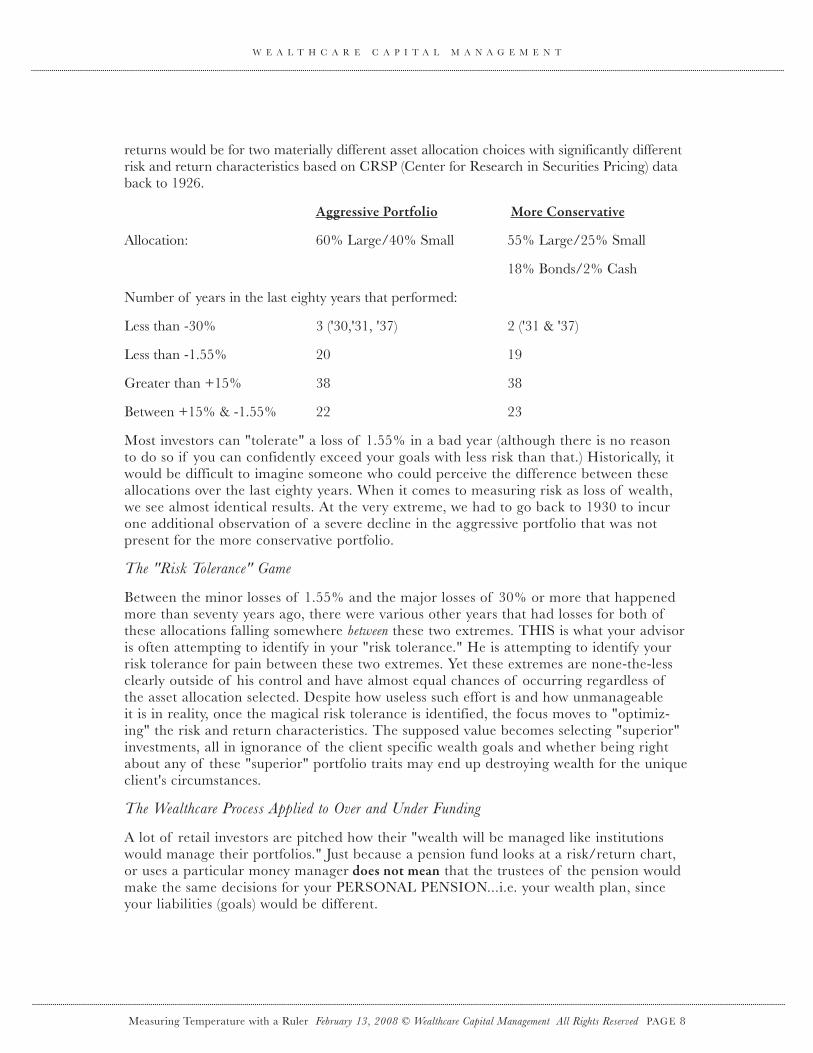
her death, despite a Great Depression that causes no reaction by the widow. But, what if her husband died one year earlier? How much impact would that have?

table 6


Table 6: Initial Advice for Widow and History's Results- Husband Passes One Year Earlier


ValueSpending


Exposure1926 20 100,000$ (5,000)$ $ 694,7 7.50% 102,495.51$ Bal Growth 80%1927 21 102,496$ (5,150)$ 27,694$ 27.02% 125,039.46$ Bal Growth 80%1928 22 125,039$ (5,305)$ 42,695$ 34.15% 162,429.87$ Bal Growth 80%1929 23 162,430$ (5,464)$ (26,461)$ -16.29% 130,505.06$ Bal Growth 80%1930 24 130,505$ (5,628)$ (28,676)$ -21.97% 96,201.58$ Bal Growth 80%1931 25 96,202$ (5,796)$ (35,277)$ -36.67% 55,128.37$ Bal Growth 80%1932 26 55,128$ (5,970)$ (2,342)$ -4.25% 46,816.16$ Bal Growth 80%1933 27 46,816$ (6,149)$ 30,780$ 65.75% 71,446.51$ Bal Growth 80%1934 28 71,447$ (6,334)$ $ 919,4 6.88% 70,031.65$ Bal Growth 80%1935 29 70,032$ (6,524)$ 26,283$ 37.53% 89,791.23$ Bal Growth 80%1936 30 89,791$ (6,720)$ 31,795$ 35.41% 114,866.96$ Bal Growth 80%1937 31 114,867$ (6,921)$ (38,457)$ -33.48% 69,488.45$ Bal Growth 80%1938 32 69,488$ (7,129)$ 18,371$ 26.44% 80,730.81$ Bal Growth 80%1939 33 80,731$ (7,343)$ $ 545 0.68% 73,933.45$ Bal Growth 80%1940 34 73,933$ (7,563)$ (4,537)$ -6.14% 61,833.14$ Bal Growth 80%1941 35 61,833$ (7,790)$ (5,278)$ -8.54% 48,765.63$ Bal Growth 80%1942 36 48,766$ (8,024)$ 11,054$ 22.67% 51,796.25$ Bal Growth 80%1943 37 51,796$ (8,264)$ 19,087$ 36.85% 62,619.42$ Bal Growth 80%1944 38 62,619$ (8,512)$ 15,420$ 24.62% 69,526.80$ Bal Growth 80%1945 39 69,527$ (8,768)$ 27,010$ 38.85% 87,769.43$ Bal Growth 80%1946 40 87,769$ (9,031)$ (6,282)$ -7.16% 72,456.62$ Bal Growth 80%1947 41 72,457$ (9,301)$ $ 765,2 3.54% 65,721.70$ Bal Growth 80%1948 42 65,722$ (9,581)$ $ 178,1 2.85% 58,011.90$ Bal Growth 80%1949 43 58,012$ (9,868)$ $ 611,9 15.71% 57,259.47$ Bal Growth 80%1950 44 57,259$ (10,164)$ $ 026,51 27.28% 62,715.32$ Bal Growth 80%1951 45 62,715$ (10,469)$ 9,567$ 15.25% 61,813.61$ Bal Growth 80%1952 46 61,814$ (10,783)$ 6,914$ 11.19% 57,945.09$ Bal Growth 80%1953 47 57,945$ (11,106)$ (897)$ -1.55% 45,941.91$ Bal Growth 80%1954 48 45,942$ (11,440)$ $ 584,02 44.59% 54,987.22$ Bal Growth 80%1955 49 54,987$ (11,783)$ $ 803,21 22.38% 55,512.78$ Bal Growth 80%1956 50 55,513$ (12,136)$ 2,581$ 4.65% 45,957.75$ Bal Growth 80%1957 51 45,958$ (12,500)$ (3,722)$ -8.10% 29,735.15$ Bal Growth 80%1958 52 29,735$ (12,875)$ $ 658,11 39.87% 28,715.31$ Bal Growth 80%1959 53 28,715$ (13,262)$ 3,062$ 10.66% 18,515.72$ Bal Growth 80%1960 54 18,516$ (13,660)$ 297$ 1.60% 5,153.34$ Bal Growth 80%1961 55 5,153$ (14,069)$ 1,195$ 23.19% BROKE Bal Growth 80%1962 56 BROKE (14,491)$ 519$ -6.72% Bal Growth 80%1963 57 (14,926)$ 18.79% Bal Growth 80%1964 58 (15,374)$ 15.74% Bal Growth 80%1965 59 (15,835)$ 17.55% Bal Growth 80%1966 60 (16,310)$ -6.35% Bal Growth 80%1967 61 (16,799)$ 34.34% Bal Growth 80%1968 62 (17,303)$ 16.00% Bal Growth 80%1969 63 (17,823)$ -10.94% Bal Growth 80%1970 64 (18,357)$ 1.01% Bal Growth 80%1971 65 (18,908)$ 13.65% Bal Growth 80%1972 66 (19,475)$ 12.55% Bal Growth 80%1973 67 (20,059)$ -14.82% Bal Growth 80%1974 68 (20,661)$ -18.36% Bal Growth 80%1975 69 (21,281)$ 35.19% Bal Growth 80%1976 70 (21,920)$ 29.88% Bal Growth 80%1977 71 (22,577)$ 2.75% Bal Growth 80%1978 72 (23,254)$ 10.24% Bal Growth 80%1979 73 (23,952)$ 21.95% Bal Growth 80%1980 74 (24,671)$ 28.73% Bal Growth 80%1981 75 (25,411)$ 2.77% Bal Growth 80%1982 76 (26,173)$ 24.22% Bal Growth 80%1983 77 (26,958)$ 23.81% Bal Growth 80%1984 78 (27,767)$ 4.50% Bal Growth 80%1985 79 (28,600)$ 27.67% Bal Growth 80%1986 80 (29,458)$ 14.72% Bal Growth 80%1987 81 (30,342)$ 1.18% Bal Growth 80%1988 82 (31,252)$ 16.19% Bal Growth 80%1989 83 (32,190)$ 22.42% Bal Growth 80%1990 84 (33,155)$ -5.23% Bal Growth 80%1991 85 (34,150)$ 30.86% Bal Growth 80%1992 86 (35,174)$ 11.42% Bal Growth 80%1993 87 (36,230)$ 12.82% Bal Growth 80%1994 88 (37,317)$ 0.65% Bal Growth 80%1995 89 (38,436)$ 32.34% Bal Growth 80%1996 90 (39,589)$ 17.58% Bal Growth 80%1997 91 (40,777)$ 25.66% Bal Growth 80%1998 92 (42,000)$ 15.83% Bal Growth 80%1999 93 (43,260)$ 18.80% Bal Growth 80%2000 94 (44,558)$ -3.52% Bal Growth 80%2001 95 (45,895)$ -2.54% Bal Growth 80%2002 96 (47,271)$ -14.56% Bal Growth 80%2003 97 (48,690)$ 28.75% Bal Growth 80%2004 98 (50,150)$ 12.20% Bal Growth 80%2005 99 (51,655)$ 5.01% Bal Growth 80%2006 100 (53,204)$ 13.24% Bal Growth 80%


Moving her income need just one year earlier had the widow broke at the same time as our "stocks for the long run" portfolio. Think about the effect of this. All we are doing is moving forward the $5,000 income need by one year, the equivalent of a one time 5% under perfor-mance. Some may argue that one additional year of inflation adjusts all of the spending need, but, let's assume she could skip the first year inflation adjustment to remove that from the equa-tion.

table 7


Table 7:Initial Advice for Widow and History's Results- Husband Passes One Year Earlier, Skip 1st Year Inflation Adj


ValueSpending


Exposure1926 20 100,000$ (5,000)$ 7,496$ 7.50% 102,495.51$ Bal Growth 80%1927 21 102,496$ (5,000)$ 27,694$ 27.02% 125,189.46$ Bal Growth 80%1928 22 125,189$ (5,150)$ 42,746$ 34.15% 162,785.59$ Bal Growth 80%1929 23 162,786$ (5,305)$ (26,519)$ -16.29% 130,961.96$ Bal Growth 80%1930 24 130,962$ (5,464)$ (28,776)$ -21.97% 96,722.00$ Bal Growth 80%1931 25 96,722$ (5,628)$ (35,468)$ -36.67% 55,626.78$ Bal Growth 80%1932 26 55,627$ (5,796)$ (2,363)$ -4.25% 47,467.29$ Bal Growth 80%1933 27 47,467$ (5,970)$ 31,208$ 65.75% 72,704.83$ Bal Growth 80%1934 28 72,705$ (6,149)$ 5,006$ 6.88% 71,561.09$ Bal Growth 80%1935 29 71,561$ (6,334)$ 26,857$ 37.53% 92,084.70$ Bal Growth 80%1936 30 92,085$ (6,524)$ 32,607$ 35.41% 118,168.26$ Bal Growth 80%1937 31 118,168$ (6,720)$ (39,563)$ -33.48% 71,886.06$ Bal Growth 80%1938 32 71,886$ (6,921)$ 19,005$ 26.44% 83,969.93$ Bal Growth 80%1939 33 83,970$ (7,129)$ 567$ 0.68% 77,408.32$ Bal Growth 80%1940 34 77,408$ (7,343)$ (4,751)$ -6.14% 65,315.04$ Bal Growth 80%1941 35 65,315$ (7,563)$ (5,575)$ -8.54% 52,177.21$ Bal Growth 80%1942 36 52,177$ (7,790)$ 11,827$ 22.67% 56,214.87$ Bal Growth 80%1943 37 56,215$ (8,024)$ 20,716$ 36.85% 68,907.05$ Bal Growth 80%1944 38 68,907$ (8,264)$ 16,968$ 24.62% 77,610.64$ Bal Growth 80%1945 39 77,611$ (8,512)$ 30,151$ 38.85% 99,249.09$ Bal Growth 80%1946 40 99,249$ (8,768)$ (7,104)$ -7.16% 83,377.62$ Bal Growth 80%1947 41 83,378$ (9,031)$ 2,953$ 3.54% 77,300.46$ Bal Growth 80%1948 42 77,300$ (9,301)$ 2,200$ 2.85% 70,199.29$ Bal Growth 80%1949 43 70,199$ (9,581)$ 11,031$ 15.71% 71,649.30$ Bal Growth 80%1950 44 71,649$ (9,868)$ 19,545$ 27.28% 81,326.59$ Bal Growth 80%1951 45 81,327$ (10,164)$ 12,406$ 15.25% 83,568.95$ Bal Growth 80%1952 46 83,569$ (10,469)$ 9,348$ 11.19% 82,448.02$ Bal Growth 80%1953 47 82,448$ (10,783)$ (1,276)$ -1.55% 70,389.14$ Bal Growth 80%1954 48 70,389$ (11,106)$ 31,386$ 44.59% 90,668.37$ Bal Growth 80%1955 49 90,668$ (11,440)$ 20,295$ 22.38% 99,524.01$ Bal Growth 80%1956 50 99,524$ (11,783)$ 4,628$ 4.65% 92,368.94$ Bal Growth 80%1957 51 92,369$ (12,136)$ (7,481)$ -8.10% 72,751.51$ Bal Growth 80%1958 52 72,752$ (12,500)$ 29,006$ 39.87% 89,257.54$ Bal Growth 80%1959 53 89,258$ (12,875)$ 9,518$ 10.66% 85,900.21$ Bal Growth 80%1960 54 85,900$ (13,262)$ 1,379$ 1.60% 74,017.08$ Bal Growth 80%1961 55 74,017$ (13,660)$ 17,162$ 23.19% 77,519.16$ Bal Growth 80%1962 56 77,519$ (14,069)$ (5,209)$ -6.72% 58,240.46$ Bal Growth 80%1963 57 58,240$ (14,491)$ 10,943$ 18.79% 54,692.26$ Bal Growth 80%1964 58 54,692$ (14,926)$ 8,611$ 15.74% 48,377.24$ Bal Growth 80%1965 59 48,377$ (15,374)$ 8,489$ 17.55% 41,492.71$ Bal Growth 80%1966 60 41,493$ (15,835)$ (2,634)$ -6.35% 23,023.32$ Bal Growth 80%1967 61 23,023$ (16,310)$ 7,907$ 34.34% 14,620.38$ Bal Growth 80%1968 62 14,620$ (16,799)$ 2,339$ 16.00% 159.72$ Bal Growth 80%1969 63 160$ (17,303)$ (17)$ -10.94% BROKE Bal Growth 80%1970 64 BROKE (17,823)$ 1.01% Bal Growth 80%1971 65 (18,357)$ 13.65% Bal Growth 80%1972 66 (18,908)$ 12.55% Bal Growth 80%1973 67 (19,475)$ -14.82% Bal Growth 80%1974 68 (20,059)$ -18.36% Bal Growth 80%1975 69 (20,661)$ 35.19% Bal Growth 80%1976 70 (21,281)$ 29.88% Bal Growth 80%1977 71 (21,920)$ 2.75% Bal Growth 80%1978 72 (22,577)$ 10.24% Bal Growth 80%1979 73 (23,254)$ 21.95% Bal Growth 80%1980 74 (23,952)$ 28.73% Bal Growth 80%1981 75 (24,671)$ 2.77% Bal Growth 80%1982 76 (25,411)$ 24.22% Bal Growth 80%1983 77 (26,173)$ 23.81% Bal Growth 80%1984 78 (26,958)$ 4.50% Bal Growth 80%1985 79 (27,767)$ 27.67% Bal Growth 80%1986 80 (28,600)$ 14.72% Bal Growth 80%1987 81 (29,458)$ 1.18% Bal Growth 80%1988 82 (30,342)$ 16.19% Bal Growth 80%1989 83 (31,252)$ 22.42% Bal Growth 80%1990 84 (32,190)$ -5.23% Bal Growth 80%1991 85 (33,155)$ 30.86% Bal Growth 80%1992 86 (34,150)$ 11.42% Bal Growth 80%1993 87 (35,174)$ 12.82% Bal Growth 80%1994 88 (36,230)$ 0.65% Bal Growth 80%1995 89 (37,317)$ 32.34% Bal Growth 80%1996 90 (38,436)$ 17.58% Bal Growth 80%1997 91 (39,589)$ 25.66% Bal Growth 80%1998 92 (40,777)$ 15.83% Bal Growth 80%1999 93 (42,000)$ 18.80% Bal Growth 80%2000 94 (43,260)$ -3.52% Bal Growth 80%2001 95 (44,558)$ -2.54% Bal Growth 80%2002 96 (45,895)$ -14.56% Bal Growth 80%2003 97 (47,271)$ 28.75% Bal Growth 80%2004 98 (48,690)$ 12.20% Bal Growth 80%2005 99 (50,150)$ 5.01% Bal Growth 80%2006 100 (51,655)$ 13.24% Bal Growth 80%


Skipping a 3% inflation adjustment to our widow's spending need oNCE over the course of the last 80 years delayed the depletion of her portfolio by eight years. THIS is why wealth managers constantly tweak their advice. It is also why I get so frustrated with active RETURN managers that argue they should measure temperature with a ruler. The difference of a one time 5% under performance was the difference between her maintaining the spending policy over her entire life along with maintaining the purchasing power of her portfolio versus being broke 44 years earlier! Can you afford to take that risk?

Any attempt to exceed the market's results will introduce a risk of potentially under performing as well, and as we can see from the example above, just oNE YEAR of inferior results can cost you 44 YEARS of lifestyle, depending on when it happens. out performing could also buy you a superior lifestyle, PRovIDED that you act upon it and do not introduce the risk of under performing after having received the benefit of your lucky or skillful superior results. However, return managers cannot control WHEN superior or inferior results will occur. That is why they measure and manage returns, and NoT wealth. So why take these bets in the first place if you don't need to? The real wealth manager does not.

We see this effect in our original case study where a return manager outperforming by 1.5% a year with certainty each and every year (no risk of under performing the benchmark in ANY year) ended up costing the widow millions. Contrast this to a wealth manager who adjusted only the allocation based on funded status in a portfolio that only equaled the index results.

Remember that all of these results are fictitious from the perspective of a real wealth manager because the oNLY thing that is changed is the allocation risk-level of the investment policy. Real wealth managers would treat the wealth management plan like a prudent pension fiducia-ry would, adjusting funding, spending, terminal values and allocation in various combinations in a continuous advising process based upon what the investor personally values.

We also know that despite using real historical returns, none of the scenarios where the widow "went broke" would have actually occurred either. The widow would have intuitively become more conservative in her spending policy and adjusted her lifestyle with or without a wealth manager to guide the way. But, such scare tactics do help return managers maximize the fees they can earn on excessively large portfolios!

If we look at exhibit one, that documents the returns, dollar values, and spending need used in all of the calculations as well as the confidence levels and the nine shifts of allocation policy that would have been made along the way for our widow (erroneously assuming the only choice exposed was allocation policy), we see some interesting things.

First, one might observe that despite the multi-billion dollar range of uncertainty we exposed in part three with a forever unchanging allocation and spending policy, we see that there were only two years in the last eighty (widow's age 27 and 28 during the Great Depression) where the confidence level for the plan couldn't be adjusted to targeted adequate funding levels by shift-ing only the asset allocation (other than the over funding periods in the last 60 years). Clearly in such an environment, the spending policy would, and SHoULD be adjusted.



exhibit one - wealth Management allocation OnLY Shifts for widow


Exhibit one- Wealth Management Allocation ONLY Shifts for Widow

Widow's Age

Beginning Value

Spending Need Return in $ Return in %

Year End Value

Change to This FWC Allocation

at Year EndConfidence

Level

Level on New

Allocationuity

posure21 100,000$ (5,000)$ 7,496$ 7.50% 102,496$ Bal Growth 83 80%22 102,496$ (5,150)$ 27,694$ 27.02% 125,039$ Bal Growth 84 80%23 125,039$ (5,305)$ 24,602$ 19.68% 144,337$ Bal Income 91 83 45%24 144,337$ (5,464)$ (3,949)$ -2.74% 134,924$ Risk Averse 92 83 30%25 134,924$ (5,628)$ (13,105)$ -9.71% 116,191$ Bal Income 73 86 45%26 116,191$ (5,796)$ (42,607)$ -36.67% 67,788$ Bal Growth 68 83 80%27 67,788$ (5,970)$ (4,794)$ -7.07% 57,024$ Aggressive 35 50 100%28 57,024$ (6,149)$ 51,060$ 89.54% 101,934$ Aggressive 31 100%29 101,934$ (6,334)$ 8,994$ 8.82% 104,595$ Aggressive 75 100%30 104,595$ (6,524)$ 46,732$ 44.68% 144,802$ Aggressive 77 100%31 144,802$ (6,720)$ 67,003$ 46.27% 205,086$ Aggressive 88 100%32 205,086$ (6,921)$ (24,283)$ -11.84% 173,882$ Risk Averse 97 94 30%33 173,882$ (7,129)$ 23,023$ 13.24% 189,776$ Risk Averse 78 30%34 189,776$ (7,343)$ 5,065$ 2.67% 187,499$ Risk Averse 83 30%35 187,499$ (7,563)$ (1,303)$ -0.70% 178,633$ Risk Averse 80 30%36 178,633$ (7,790)$ (8,176)$ -4.58% 162,667$ Bal Income 71 85 45%37 162,667$ (8,024)$ 28,893$ 17.76% 183,536$ Balanced 72 81 60%38 183,536$ (8,264)$ 53,381$ 29.08% 228,653$ Balanced 87 60%39 228,653$ (8,512)$ 23,855$ 10.43% 243,996$ Risk Averse 95 87 30%40 243,996$ (8,768)$ 39,070$ 16.01% 274,299$ Risk Averse 90 30%41 274,299$ (9,031)$ (5,867)$ -2.14% 259,402$ Risk Averse 95 30%42 259,402$ (9,301)$ 4,747$ 1.83% 254,847$ Risk Averse 91 30%43 254,847$ (9,581)$ 5,298$ 2.08% 250,564$ Risk Averse 89 30%44 250,564$ (9,868)$ 18,135$ 7.24% 258,831$ Risk Averse 84 30%45 258,831$ (10,164)$ 27,844$ 10.76% 276,511$ Risk Averse 86 30%46 276,511$ (10,469)$ 16,453$ 5.95% 282,495$ Risk Averse 89 30%47 282,495$ (10,783)$ 14,469$ 5.12% 286,180$ Risk Averse 89 30%48 286,180$ (11,106)$ 3,650$ 1.28% 278,723$ Risk Averse 89 30%49 278,723$ (11,440)$ 50,947$ 18.28% 318,231$ Risk Averse 85 30%50 318,231$ (11,783)$ 25,852$ 8.12% 332,300$ Risk Averse 92 30%51 332,300$ (12,136)$ 5,758$ 1.73% 325,922$ Risk Averse 93 30%52 325,922$ (12,500)$ 4,574$ 1.40% 317,996$ Risk Averse 91 30%53 317,996$ (12,875)$ 46,244$ 14.54% 351,365$ Risk Averse 90 30%54 351,365$ (13,262)$ 14,377$ 4.09% 352,480$ Risk Averse 93 30%55 352,480$ (13,660)$ 24,972$ 7.08% 363,793$ Risk Averse 92 30%56 363,793$ (14,069)$ 36,047$ 9.91% 385,771$ Risk Averse 92 30%57 385,771$ (14,491)$ 2,607$ 0.68% 373,887$ Risk Averse 95 30%58 373,887$ (14,926)$ 30,707$ 8.21% 389,667$ Risk Averse 91 30%59 389,667$ (15,374)$ 32,843$ 8.43% 407,136$ Risk Averse 95 30%60 407,136$ (15,835)$ 31,225$ 7.67% 422,526$ Risk Averse 96 30%61 422,526$ (16,310)$ 2,429$ 0.57% 408,645$ Risk Averse 96 30%62 408,645$ (16,799)$ 57,939$ 14.18% 449,784$ Risk Averse 93 30%63 449,784$ (17,303)$ 40,710$ 9.05% 473,190$ Risk Averse 97 30%64 473,190$ (17,823)$ (18,879)$ -3.99% 436,489$ Risk Averse 98 30%65 436,489$ (18,357)$ 42,888$ 9.83% 461,020$ Risk Averse 93 30%66 461,020$ (18,908)$ 46,948$ 10.18% 489,060$ Risk Averse 95 30%67 489,060$ (19,475)$ 37,747$ 7.72% 507,332$ Risk Averse 98 30%68 507,332$ (20,059)$ (13,018)$ -2.57% 474,254$ Risk Averse 99 30%69 474,254$ (20,661)$ (14,578)$ -3.07% 439,014$ Risk Averse 96 30%70 439,014$ (21,281)$ 79,028$ 18.00% 496,761$ Risk Averse 90 30%71 496,761$ (21,920)$ 93,075$ 18.74% 567,917$ Risk Averse 96 30%72 567,917$ (22,577)$ 13,952$ 2.46% 559,292$ Risk Averse 99 30%73 559,292$ (23,254)$ 36,176$ 6.47% 572,214$ Risk Averse 99 30%74 572,214$ (23,952)$ 65,966$ 11.53% 614,228$ Risk Averse 99 30%75 614,228$ (24,671)$ 85,627$ 13.94% 675,184$ Risk Averse 100 30%76 675,184$ (25,411)$ 50,975$ 7.55% 700,749$ Risk Averse 100 30%77 700,749$ (26,173)$ 179,354$ 25.59% 853,930$ Risk Averse 100 30%78 853,930$ (26,958)$ 117,784$ 13.79% 944,756$ Risk Averse 100 30%79 944,756$ (27,767)$ 94,309$ 9.98% 1,011,297$ Risk Averse 100 30%80 1,011,297$ (28,600)$ 221,160$ 21.87% 1,203,857$ Risk Averse 100 30%81 1,203,857$ (29,458)$ 169,492$ 14.08% 1,343,890$ Risk Averse 100 30%82 1,343,890$ (30,342)$ 32,325$ 2.41% 1,345,874$ Risk Averse 100 30%83 1,345,874$ (31,252)$ 133,851$ 9.95% 1,448,473$ Risk Averse 100 30%84 1,448,473$ (32,190)$ 233,575$ 16.13% 1,649,858$ Risk Averse 100 30%85 1,649,858$ (33,155)$ 63,169$ 3.83% 1,679,871$ Risk Averse 100 30%86 1,679,871$ (34,150)$ 342,864$ 20.41% 1,988,585$ Risk Averse 100 30%87 1,988,585$ (35,174)$ 169,701$ 8.53% 2,123,111$ Risk Averse 100 30%88 2,123,111$ (36,230)$ 236,288$ 11.13% 2,323,170$ Risk Averse 100 30%89 2,323,170$ (37,317)$ (49,343)$ -2.12% 2,236,511$ Risk Averse 100 30%90 2,236,511$ (38,436)$ 482,447$ 21.57% 2,680,522$ Risk Averse 100 30%91 2,680,522$ (39,589)$ 218,691$ 8.16% 2,859,624$ Risk Averse 100 30%92 2,859,624$ (40,777)$ 414,742$ 14.50% 3,233,590$ Risk Averse 100 30%93 3,233,590$ (42,000)$ 374,943$ 11.60% 3,566,533$ Risk Averse 100 30%94 3,566,533$ (43,260)$ 235,149$ 6.59% 3,758,422$ Risk Averse 100 30%95 3,758,422$ (44,558)$ 224,077$ 5.96% 3,937,941$ Risk Averse 100 30%96 3,937,941$ (45,895)$ 69,442$ 1.76% 3,961,488$ Risk Averse 100 30%97 3,961,488$ (47,271)$ 136,117$ 3.44% 4,050,334$ Risk Averse 100 30%98 4,050,334$ (48,690)$ 461,252$ 11.39% 4,462,896$ Risk Averse 100 30%99 4,462,896$ (50,150)$ 335,699$ 7.52% 4,748,445$ Risk Averse 100 30%

100 4,748,445$ (51,655)$ 181,732$ 3.83% 4,878,522$ Risk Averse 100 30%

EqEx


We also observe how unrealistic this is, because it assumes the widow wouldn't adjust her spending at the young age of 59, despite having excessive confidence and a spending need of only 3.7% of the CURRENT portfolio value. It only gets worse from there. By age 80 she would only be spending 2.8% of the portfolio value and by age 99 she would be at only 1%. In reality, a real wealth manager would have told her to spend more.

of course, this is what would happen if people really never thought about things, but they do, which is what makes an assumption there would be no adjustments over a lifetime so unrealis-tic.

So, what were the returns and portfolio values for the other allocation choices? Was it a Black Swan with a fat tail that swooped down upon the portfolio that caused most of the other allo-cation choices to "fail?" Was there an outlier in the bell curve (by the way, our bell is warped because we use a log normal distribution, not a normal distribution) that caused the other allo-cations to "fail," like our initial plan would have if the timing of her husband's death moved by only one year?

exhibit two shows us the returns for each year, for the five allocation choices for our widow. one would notice in the shaded area that there were not outlier returns immediately preceding the time periods where the widow ran out of money with these choices. Well...maybe there were outliers, but they were more likely to the upside, not downside. The WoRST loss of any of these portfolios in the shaded area was a 100% stock allocation with a 10.78% decline. That is hardly a "Black Swan." Two of the seven years before the widow ran out of money with the "#1-Stocks for the Long Run" allocation, she would have experienced returns of more than 40%!



exhibit two - returns for the allocation choices


Exhibit two- Returns for the allocation choicesAsset Allocation Alternatives- Returns

Widow's Age

#1- Long Term (Risk "Tolerance")

Allocation

#2- Age Based Allocation (Target

Date)#3- Stocks for the Long Run

# 4- Superior Selection

#5- Wealth Management

Allocation21 5.96% 6.68% 11.62% 7.46% 7.50%22 14.55% 25.66% 37.49% 16.05% 27.02%23 16.45% 33.08% 43.61% 17.95% 19.68%24 -5.90% -18.36% -8.42% -4.40% -2.74%25 -7.28% -21.47% -24.90% -5.78% -9.71%26 -18.59% -34.91% -43.34% -17.09% -36.67%27 2.61% -3.18% -8.19% 4.11% -7.07%28 34.73% 65.81% 53.99% 36.23% 89.54%29 8.67% 8.61% -1.44% 10.17% 8.82%30 20.95% 33.55% 47.67% 22.45% 44.68%31 19.20% 33.22% 33.92% 20.70% 46.27%32 -15.67% -30.07% -35.03% -14.17% -11.84%33 15.64% 23.43% 31.12% 17.14% 13.24%34 2.65% 1.29% -0.41% 4.15% 2.67%35 -1.22% -4.32% -9.78% 0.28% -0.70%36 -3.67% -6.70% -11.59% -2.17% -4.58%37 12.43% 19.85% 20.34% 13.93% 17.76%38 20.80% 33.03% 25.90% 22.30% 29.08%39 13.60% 21.31% 19.75% 15.10% 10.43%40 20.60% 32.11% 36.44% 22.10% 16.01%41 -2.96% -5.31% -8.07% -1.46% -2.14%42 1.98% 2.60% 5.71% 3.48% 1.83%43 2.05% 2.17% 5.50% 3.55% 2.08%44 8.62% 11.89% 18.79% 10.12% 7.24%45 13.42% 19.66% 31.71% 14.92% 10.76%46 6.85% 9.84% 24.02% 8.35% 5.95%47 5.61% 7.36% 18.37% 7.11% 5.12%48 0.78% -0.21% -0.99% 2.28% 1.28%49 22.58% 30.25% 52.62% 24.08% 18.28%50 9.85% 13.58% 31.56% 11.35% 8.12%51 1.94% 2.70% 6.56% 3.44% 1.73%52 0.13% -2.17% -10.78% 1.63% 1.40%53 18.80% 24.36% 43.36% 20.30% 14.54%54 5.01% 6.35% 11.96% 6.51% 4.09%55 6.68% 5.60% 0.47% 8.18% 7.08%56 12.04% 14.06% 26.89% 13.54% 9.91%57 -0.37% -1.37% -8.73% 1.13% 0.68%58 9.75% 10.92% 22.80% 11.25% 8.21%59 9.76% 10.44% 16.48% 11.26% 8.43%60 9.80% 10.60% 12.45% 11.30% 7.67%61 -0.39% -0.72% -10.06% 1.11% 0.57%62 18.69% 19.36% 23.98% 20.19% 14.18%63 10.75% 10.82% 11.06% 12.25% 9.05%64 -5.92% -5.84% -8.50% -4.42% -3.99%65 8.50% 8.83% 4.01% 10.00% 9.83%66 11.02% 10.85% 14.31% 12.52% 10.18%67 8.12% 7.84% 18.98% 9.62% 7.72%68 -5.00% -3.83% -14.66% -3.50% -2.57%69 -5.34% -3.70% -26.47% -3.84% -3.07%70 21.15% 18.81% 37.20% 22.65% 18.00%71 21.80% 19.95% 23.84% 23.30% 18.74%72 3.18% 2.80% -7.18% 4.68% 2.46%73 7.29% 6.35% 6.56% 8.79% 6.47%74 13.43% 10.86% 18.44% 14.93% 11.53%75 15.96% 12.32% 32.42% 17.46% 13.94%76 7.04% 7.90% -4.91% 8.54% 7.55%77 26.64% 27.33% 21.41% 28.14% 25.59%78 15.70% 12.50% 22.51% 17.20% 13.79%79 9.04% 11.05% 6.27% 10.54% 9.98%80 23.27% 21.81% 32.16% 24.77% 21.87%81 14.38% 14.61% 18.47% 15.88% 14.08%82 1.67% 2.32% 5.23% 3.17% 2.41%83 11.04% 8.47% 16.81% 12.54% 9.95%84 16.78% 14.79% 31.49% 18.28% 16.13%85 2.06% 6.43% -3.17% 3.56% 3.83%86 22.95% 18.27% 30.55% 24.45% 20.41%87 9.62% 8.02% 7.67% 11.12% 8.53%88 12.17% 11.40% 9.99% 13.67% 11.13%89 -2.18% -4.01% 1.31% -0.68% -2.12%90 23.77% 18.60% 37.43% 25.27% 21.57%91 9.25% 4.07% 23.07% 10.75% 8.16%92 16.08% 10.15% 33.36% 17.58% 14.50%93 11.56% 10.37% 28.58% 13.06% 11.60%94 8.31% 0.26% 21.04% 9.81% 6.59%95 5.07% 11.22% -9.11% 6.57% 5.96%96 1.76% 3.74% -11.88% 3.26% 1.76%97 1.57% 14.42% -22.10% 3.07% 3.44%98 14.61% 1.80% 28.69% 16.11% 11.39%99 8.73% 5.27% 10.87% 10.23% 7.52%

100 4.06% 3.12% 4.89% 5.56% 3.83%


In exhibit three we can observe the DoLLAR impact of these returns on the widow's wealth.

exhibit three - widow's portfolio value based on each of the allocation policy choices


Exhibit three- Widow’s portfolio value based on each of the allocation policy choices Asset Allocation Alternatives- Portfolio Values

Widow's Age

#1- Long Term (Risk "Tolerance")

Allocation

#2- Age Based Allocation

(Target Date)#3- Stocks for the Long Run

# 4- Superior Selection

#5- Wealth Management

Allocation21 100,955$ 101,680$ 106,624$ 102,455$ 102,496$ 22 110,496$ 122,621$ 141,446$ 113,751$ 125,039$ 23 123,364$ 157,874$ 197,823$ 128,861$ 144,337$ 24 110,626$ 123,423$ 175,712$ 117,732$ 134,924$ 25 96,946$ 91,300$ 126,338$ 105,300$ 116,191$ 26 73,128$ 53,634$ 65,791$ 81,509$ 67,788$ 27 69,066$ 45,960$ 54,431$ 78,888$ 57,024$ 28 86,903$ 70,058$ 77,668$ 101,319$ 101,934$ 29 88,100$ 69,754$ 70,214$ 105,286$ 104,595$ 30 100,035$ 86,631$ 97,160$ 122,401$ 144,802$ 31 112,526$ 108,692$ 123,399$ 141,022$ 205,086$ 32 87,967$ 69,092$ 73,255$ 114,112$ 173,882$ 33 94,600$ 78,148$ 88,925$ 126,547$ 189,776$ 34 89,764$ 71,810$ 81,217$ 124,456$ 187,499$ 35 81,106$ 61,147$ 65,707$ 117,242$ 178,633$ 36 70,341$ 49,260$ 50,300$ 106,909$ 162,667$ 37 71,061$ 51,015$ 52,508$ 113,779$ 183,536$ 38 77,574$ 59,599$ 57,843$ 130,882$ 228,653$ 39 79,612$ 63,787$ 60,757$ 142,134$ 243,996$ 40 87,245$ 75,498$ 74,127$ 164,779$ 274,299$ 41 75,634$ 62,456$ 59,113$ 153,346$ 259,402$ 42 67,830$ 54,777$ 53,186$ 149,381$ 254,847$ 43 59,637$ 46,385$ 46,531$ 145,096$ 250,564$ 44 54,908$ 42,033$ 45,408$ 149,907$ 258,831$ 45 52,113$ 40,132$ 49,644$ 162,112$ 276,511$ 46 45,212$ 33,612$ 51,098$ 165,171$ 282,495$ 47 36,967$ 25,302$ 49,700$ 166,140$ 286,180$ 48 26,148$ 14,142$ 38,102$ 158,819$ 278,723$ 49 20,614$ 6,980$ 46,713$ 185,627$ 318,231$ 50 10,861$ BROKE 49,674$ 194,904$ 332,300$ 51 BROKE 40,794$ 189,481$ 325,922$ 52 23,895$ 180,077$ 317,996$ 53 21,382$ 203,762$ 351,365$ 54 10,676$ 203,774$ 352,480$ 55 BROKE 206,781$ 363,793$ 56 220,719$ 385,771$ 57 208,729$ 373,887$ 58 217,282$ 389,667$ 59 226,370$ 407,136$ 60 236,121$ 422,526$ 61 222,426$ 408,645$ 62 250,525$ 449,784$ 63 263,909$ 473,190$ 64 234,419$ 436,489$ 65 239,503$ 461,020$ 66 250,580$ 489,060$ 67 255,223$ 507,332$ 68 226,225$ 474,254$ 69 196,877$ 439,014$ 70 220,186$ 496,761$ 71 249,562$ 567,917$ 72 238,673$ 559,292$ 73 236,401$ 572,214$ 74 247,746$ 614,228$ 75 266,328$ 675,184$ 76 263,661$ 700,749$ 77 311,692$ 853,930$ 78 338,345$ 944,756$ 79 346,232$ 1,011,297$ 80 403,391$ 1,203,857$ 81 437,974$ 1,343,890$ 82 421,524$ 1,345,874$ 83 443,142$ 1,448,473$ 84 491,939$ 1,649,858$ 85 476,312$ 1,679,871$ 86 558,618$ 1,988,585$ 87 585,539$ 2,123,111$ 88 629,358$ 2,323,170$ 89 587,768$ 2,236,511$ 90 697,842$ 2,680,522$ 91 733,293$ 2,859,624$ 92 821,423$ 3,233,590$ 93 886,667$ 3,566,533$ 94 930,359$ 3,758,422$ 95 946,901$ 3,937,941$ 96 931,920$ 3,961,488$ 97 913,283$ 4,050,334$ 98 1,011,722$ 4,462,896$ 99 1,065,108$ 4,748,445$

100 1,072,678$ 4,878,522$


So what does all of this data mean? Does it mean that we will always produce more wealth with a real wealth management approach as opposed to a return management approach? No, it doesn't. In retrospect there will always be better decisions that could have been made. That does not make it rational to project making superior decisions in the future while ignoring the uncertainty such decisions introduce.

Does it mean that measuring and managing funded status is a better "market timing" strategy that produces superior returns? No, it doesn't, because the funded status is unique to each indi-vidual's cash flows and risk capacity and in reality there will be many more changes made than just the asset allocation.

This merely means there is a vast amount of uncertainty in the market's behavior. Think about the multi-billion dollar range of uncertainty for our widow with $100,000. when different results occur affects different people in different ways, sometimes with no effect, and sometimes with an effect that would cause a change to something other than their allocation. Why are planners so stuck on being able to forecast things? Clients WANT advice about their choices to improve their lifestyle because of Green Swans, or prudent tweaks they should make in the face of possible Black Swans.

Return managers measure something that is often meaningless to wealth. They may or may not be successful at producing superior risk adjusted returns. But, it may be irrelevant in terms of actual wealth a person has, or can spend.

The abuses of the "odds of success" crowd cost many investors dearly. They focus only on find-ing Black Swans (not green ones, where there is more wealth and choices.) But it is time to stop playing these ridiculous games by pretending that 85% or 90% confidence is "better" than 83% or 75%. There are so many SMALL, tiny, insignificant savings and spending policy decisions that are far more manageable than the vast continuous uncertainty of the markets, and these decision levers are what real wealth managers can utilize to provide realistic and meaningful advice. That DoES NoT mean the advice will never change.

The future of financial advising is dependent on advisors recognizing this. Do you?



Part Five - Conclusion: Superior Results with True Wealth Management

"Most people would rather be certain they're miserable than risk being happy."

robert anthony

In part one of this paper, we showed some simple examples of the effects of the difference between time weighted returns (return managers) versus dollar weighted (wealth manager) returns. Part two went through a real life client example and demonstrated how some of the "best" generally accepted and even clairvoyantly "successful" approaches of asset allocation ended up costing a widow investor millions of dollars of wealth. Part three examined how unlike-ly it is that markets would behave in a manner that would have avoided over and under fund-ing, even though the initial odds were very high. Part four provided the detailed back up data for the returns and allocation shifts for our sample widow in part two. It also demonstrated how sensitive her wealth plan was to just one year of timing for a cash flow, inflation adjustment or just one year of inferior investment results.

In this last part of this paper, we will demonstrate that the superior dollar result of real wealth management is NoT due to mean reversion, lucky market timing, or exposing an investor to excessive investment risk (all assumptions of return managers, not wealth managers). To dem-onstrate this, we will apply the same rules we used for our 20 year old widow example - adjust-ing only the asset allocation but unrealistically not client goals - to another investor who is also 20 years old but is saving for a retirement that is 45 years away (referred to as "saver"). To keep a level playing field, both will start with the same 82% initial confidence level for their wealth management plan with a portfolio allocation that begins with 80% equity exposure in 1926.

The first step in this process is to examine the allocation shifts of a wealth management plan for our 20 year old saver to observe whether, like the widow, he experiences superior wealth results relative to other clairvoyantly selected "superior" investment strategies. His situation back in 1926 is that he is 20 years old and starts with $2,000 in annual savings (keep in mind this is over $21,000 in today's dollars) adjusted each year for 3% inflation until retirement at age 65, with a $103,000 inflation-adjusted retirement income to age 100. This case is very simi-lar to the "saver" we introduced in part three when we examined risk capacity relative to our widow and how unlikely it was the market would behave in a manner that would cause an allo-cation change for him in the near term, yet it was very likely for the widow. We slightly lowered the income goal for our saver in this case though to match both the initial confidence level and allocation at inception in 1926 to the widow's so we could contrast the difference in allocation shifts over time on a completely level playing field.

As would be expected for a plan with such high risk capacity, a 100% stock allocation in the "stocks for the long run portfolio" would actually almost double the results of the wealth man-agement plan. But, keep in mind, in the wealth management plan the rules we apply are to avoid needless risk exposure to the equity markets and over the life of our saver we average only 53% equity exposure versus a lifetime of being 100% exposed to equities.

Also, as might be expected for a plan with very high risk capacity, using a fixed allocation over the entire life of the plan with a 45 year accumulation period is too conservative and produces an inferior geometric mean result, albeit with very low investment risk. Despite the wealth



management plan producing only 0.46% higher compound return with 5.5% higher risk, the wealth result compounds over time to be more than 21 TIMES the wealth result of constant-weighted allocation that is unchanged over the entire plan horizon.

Also like the widow's example, the target date/lifecycle approach is once again about the worst choice that could be made for the saver. Starting with 80% equities and reducing the equity exposure by 1% a year at each birthday (as is the common rule of thumb for this approach) not only exposed our saver to fairly high risk and a low return, but had him broke at age 90 versus having $26.7 MILLIoN at the end of the wealth management plan. The theory of target date/lifecycle approaches is to use the calendar as a proxy to consider risk capacity of withdrawals, but since it ignores the funded status, the shifts in allocation will frequently go the wrong direction from what makes sense based on the market's uncertain behavior and thus is the worst dollar result for both our widow and the saver.

Unlike our widow, for our saver with extraordinarily high risk capacity, none of these results are significantly different than what would have been predicted by return managers. However, many return managers argue that their value lies in superior selection and their ability to out-perform and/or reduce investment risk. In our saver's case, his high risk capacity during much of his plan exposes a significant difference from our widow in the excess returns that need to be produced to come close to competing with a real wealth management plan. If we take the aver-age equity exposure of the real wealth management plan of 53% and assume that the superior selection skills outperform the allocation policy by 0.75% each and every year (completely ignoring the risk of ever underperforming at the wrong time for the investor) we can observe in table 8 that the higher returns and lower risk added no value, and once again cost the investor OVER $4 million of wealth.

table 8 - wealth Management Choices for our 20 year old Saver

Wealth Management Superior Selection

Compound Return 9.78% 10.07%

Risk 18.54% 12.98%

Growth of $100 $174,519 $216,166

Wealth at age 100 $26,743,678 $22,731,344

So, despite the high risk capacity and long term accumulation of our saver's wealth manage-ment plan, we again observe how misleading "successful" management of returns (and risk) is from the perspective of wealth. It is easy for return managers to sell this because investors are not aware of it, and make the erroneous assumption that there is some benefit to producing higher returns with lower risks. BUT, is having $4 million LESS WEALTH a benefit with the SAME spending?

Think about how much "conventional wisdom" has suckered financial advisors into buying this lack of any real value proposition promoted by brokerage firms, money managers and mutual fund complexes into standard "best practices."

How many times have you seen a risk versus return chart like the one below in Chart 5?



Chart 5 - historical risk versus return

The "Superior Selection" pink square on the risk/return chart shows a "great" benefit for the return managers that promote "risk adjusted returns" instead of wealth management. Sometimes return managers would sell such a portfolio based on how much it is above the effi-cient frontier, often drawing a line from the pink square straight down to the efficient frontier and showing that "excess return" as being their "value."

Even more ironic to me is how many advisors buy the story from the product vendors that are swindling them into a sales pitch that goes something like, "we are not seeking excess returns, we are about risk control and we seek investment results that only match market results with less investment risk." of course, to sell this story they use a horizontal line that goes directly right from the pink square to the efficient frontier, supposedly demonstrating that they comply with their sales pitch of only equaling efficient market results with "less risk." How can investors (or worse, sophisticated financial advisors) be suckered into buying this? It is almost like a bad magician's sleight of hand in misdirecting the attention of the observer by choosing to guide their gaze based only on whether they focus vertically (the out performance pitch) or horizon-tally (the risk control pitch.) They are the same story! They are just packaged differently!

The one thing that is not normally shown on such risk/return charts is what the WEALTH effect is to the client. In this case however we expose the fraud of the return manager sales spin by showing the ending wealth result for a specific client and the $4 million price to our saver's wealth derived from the return manager's approach of producing higher returns with lower risk. (The returns are all geometric/compound returns and the risk is standard deviation of annual returns.)

on a complete efficient frontier, there are more than just the model portfolio dots, there are an infinite number of portfolios that make up that efficient frontier line (the portfolio model "dots" are the actual results of FWC Model allocations used throughout this paper as described


Actual Allocation Risk Vs. Returns 80 Years Ending 12/31/2005And Wealth Results for "Saver" Wealth Management Plan

Aggressive Growth

Growth

Bal Growth

Balanced

Bal Income

Risk Averse

Superior Selection$22.7 Million Wealth

Management$26.7 Million

7.00%

7.50%

8.00%

8.50%

9.00%

9.50%

10.00%

10.50%

11.00%

11.50%

12.00%

7.00% 12.00% 17.00% 22.00% 27.00%

Risk (SD)

Ret

urn

(Geo

met

ric)


in footnote 3.) IF we were to choose merely the efficient portfolio that matched return for the superior selection portfolio (where the horizontal right arrow hits the efficient frontier) we would discover that such an efficient but "inferior" portfolio that had more risk and the same return would have produced $30.2 million dollars, or $7.5 million MoRE WEALTH than the less risk and same return "superior selection" portfolio! (See Chart 6, below)

Chart 6 - higher risk and Same return produce higher wealth

Likewise, demonstrating the value of true wealth management, if I chose the portfolio on the efficient frontier that matched the return of the wealth management plan but was obviously more efficient (where the arrow goes left from our green wealth management plan triangle in Chart 5) I would discover the WEALTH result to be only $16.2 million, a full $10.5 MILLIoN DoLLARS oF WEALTH less than that "inefficient" real wealth management portfolio with more risk, and the same return (see Chart 7.)


Chart 6- Higher Risk and Same Return Produce Higher Wealth


Aggressive Growth

Growth

Bal Growth

Balanced

Bal Income

Risk Averse



7.00%

7.50%

8.00%

8.50%

9.00%

9.50%

10.00%

10.50%

11.00%

11.50%

12.00%

7.00% 12.00% 17.00% 22.00% 27.00%

Risk (SD)

Retu

rn (G

eom

etric

)

Same Return & More Risk= $30.5 Million


Aggressive Growth

Growth

Bal Growth

Balanced

Bal Income

Risk Averse



7.00%

7.50%

8.00%

8.50%

9.00%

9.50%

10.00%

10.50%

11.00%

11.50%

12.00%

7.00% 12.00% 17.00% 22.00% 27.00%

Risk (SD)

Retu

rn (G

eom

etric

)

Same Return & More Risk= $30.5 Million


Chart 7 - Same return and Lower risk produce Less wealth

It is personally very frustrating to me to see how such charts are used every day in the invest-ment product selling industry to demonstrate fictitious value and also used to justify vastly uncertain choices in product selection (often with certain high expenses.) When one con-siders that the way such sales presentations are normally assembled is based on uncertain future results based on track record of what happened, instead of WHAT WoULD HAvE HAPPENED as in this analysis, it makes me want to scream!

The bottom line of this contrast though is the reality of what we showed in the widow's case, our saver's case, and where we started this entire series; it is the premise of the fundamental dif-ference between managing returns, and managing wealth.

Personally, I am confused as to why people don't get this. To me it does not seem complicated to understand the simple realities of the difference in these two approaches. I know it is concep-tually easier to ignore the reality of the numerous year by year variable results and data points to an oversimplified "bottom line" risk and return number. But, when we know that doing so may be meaningless for what one is trying to achieve, you would think that there would be a large enough universe of advisors out there who are sophisticated enough to expose the fallacy so that the game would ultimately come to an end. Yet, currently it thrives and even grows despite the fiction on which it is based.

Were these two superior wealth results of the widow and saver due to "mean reversion" or exceptionally lucky timing? or, is this merely the nature of continuously managing the future uncertainty based on a unique set of goals (liability stream) as competently managed pension trusts do?


Chart 7- Same Return and Lower Risk Produce Less Wealth


Aggressive Growth

Growth

Bal Growth

Balanced

Bal Income

Risk Averse



7.00%

7.50%

8.00%

8.50%

9.00%

9.50%

10.00%

10.50%

11.00%

11.50%

12.00%

7.00% 12.00% 17.00% 22.00% 27.00%

Risk (SD)

Retu

rn (G

eom

etric

) Same Return & Less Risk= $16.2

Million


Aggressive Growth

Growth

Bal Growth

Balanced

Bal Income

Risk Averse



7.00%

7.50%

8.00%

8.50%

9.00%

9.50%

10.00%

10.50%

11.00%

11.50%

12.00%

7.00% 12.00% 17.00% 22.00% 27.00%

Risk (SD)

Retu

rn (G

eom

etric

) Same Return & Less Risk= $16.2

Million


table 9 - Details of "Saver's" plan and allocation Shifts

As one might expect with a wealth management plan for a young saver with high risk capacity, there are fewer allocation shifts relative to the widow's plan (7 versus 9). In fact, this high risk capacity plan of our saver (see table 9) caused only oNE allocation shift in the first TWENTY years of the plan, despite a very wild Great Depression bear market and post Depression


Table 9- Details of “Saver’s” Plan and Allocation Shifts

Saver's Age Beginning Value

Savings (Spending

Need) Return in $ Return in % Year End

Value AllocationConfidence

Level

Confidence on New

AllocationEquity

Exposure21 2,000$ 2,000$ 150$ 7.5% 4,150$ Bal Growth 77 80%22 4,150$ 2,060$ 1,121$ 27.0% 7,331$ Bal Growth 79 80%23 7,331$ 2,122$ 2,503$ 34.1% 11,956$ Bal Growth 80 80%24 11,956$ 2,185$ (1,948)$ -16.3% 12,194$ Bal Growth 81 80%25 12,194$ 2,251$ (2,679)$ -22.0% 11,766$ Bal Growth 77 80%26 11,766$ 2,319$ (4,314)$ -36.7% 9,770$ Bal Growth 75 80%27 9,770$ 2,388$ (415)$ -4.2% 11,743$ Bal Growth 69 80 80%28 11,743$ 2,460$ 10,515$ 89.5% 24,717$ Aggressive 78 100%29 24,717$ 2,534$ 2,181$ 8.8% 29,432$ Aggressive 84 100%30 29,432$ 2,610$ 13,150$ 44.7% 45,191$ Aggressive 83 100%31 45,191$ 2,688$ 20,911$ 46.3% 68,789$ Aggressive 85 100%32 68,789$ 2,768$ (30,418)$ -44.2% 41,140$ Aggressive 90 100%33 41,140$ 2,852$ 13,079$ 31.8% 57,071$ Aggressive 83 100%34 57,071$ 2,937$ (62)$ -0.1% 59,946$ Aggressive 82 100%35 59,946$ 3,025$ (4,755)$ -7.9% 58,216$ Aggressive 82 100%36 58,216$ 3,116$ (6,145)$ -10.6% 55,187$ Aggressive 79 100%37 55,187$ 3,209$ 16,560$ 30.0% 74,957$ Aggressive 74 100%38 74,957$ 3,306$ 38,145$ 50.9% 116,407$ Aggressive 77 100%39 116,407$ 3,405$ 38,811$ 33.3% 158,623$ Aggressive 83 100%40 158,623$ 3,507$ 81,383$ 51.3% 243,513$ Aggressive 86 100%41 243,513$ 3,612$ (12,593)$ -5.2% 234,532$ Balanced 91 81 60%42 234,532$ 3,721$ 6,610$ 2.8% 244,863$ Balanced 77 60%43 244,863$ 3,832$ 6,087$ 2.5% 254,782$ Balanced 75 60%44 254,782$ 3,947$ 40,034$ 15.7% 298,764$ Bal Growth 70 80 80%45 298,764$ 4,066$ 81,500$ 27.3% 384,329$ Bal Growth 82 80%46 384,329$ 4,188$ 58,629$ 15.3% 447,146$ Bal Growth 84 80%47 447,146$ 4,313$ 50,017$ 11.2% 501,476$ Bal Growth 88 80%48 501,476$ 4,443$ (7,761)$ -1.5% 498,158$ Bal Growth 87 80%49 498,158$ 4,576$ 222,123$ 44.6% 724,857$ Bal Growth 85 80%50 724,857$ 4,713$ 89,073$ 12.3% 818,643$ Bal Income 91 85 45%51 818,643$ 4,855$ 20,643$ 2.5% 844,141$ Bal Income 86 45%52 844,141$ 5,000$ (11,346)$ -1.3% 837,796$ Bal Income 86 45%53 837,796$ 5,150$ 185,780$ 22.2% 1,028,726$ Bal Income 80 45%54 1,028,726$ 5,305$ 61,709$ 6.0% 1,095,740$ Bal Income 88 45%55 1,095,740$ 5,464$ 62,001$ 5.7% 1,163,205$ Bal Income 88 45%56 1,163,205$ 5,628$ 161,810$ 13.9% 1,330,642$ Bal Income 85 45%57 1,330,642$ 5,797$ (19,763)$ -1.5% 1,316,676$ Bal Income 89 45%58 1,316,676$ 5,970$ 149,461$ 11.4% 1,472,107$ Bal Income 86 45%59 1,472,107$ 6,150$ 157,098$ 10.7% 1,635,355$ Bal Income 87 45%60 1,635,355$ 6,334$ 175,047$ 10.7% 1,816,736$ Bal Income 90 45%61 1,816,736$ 6,524$ (27,046)$ -1.5% 1,796,214$ Bal Income 89 45%62 1,796,214$ 6,720$ 367,197$ 20.4% 2,170,131$ Bal Income 85 45%63 2,170,131$ 6,921$ 196,419$ 9.1% 2,373,471$ Risk Averse 92 88 30%64 2,373,471$ 7,129$ (94,696)$ -4.0% 2,285,905$ Risk Averse 89 30%65 2,285,905$ (103,000)$ 224,607$ 9.8% 2,407,511$ Risk Averse 80 30%66 2,407,511$ (106,090)$ 245,170$ 10.2% 2,546,591$ Risk Averse 82 30%67 2,546,591$ (109,273)$ 196,555$ 7.7% 2,633,874$ Risk Averse 90 30%68 2,633,874$ (112,551)$ (67,586)$ -2.6% 2,453,737$ Risk Averse 89 30%69 2,453,737$ (115,927)$ (75,427)$ -3.1% 2,262,382$ Risk Averse 78 30%70 2,262,382$ (119,405)$ 526,887$ 23.3% 2,669,865$ Bal Income 67 79 45%71 2,669,865$ (122,987)$ 599,345$ 22.4% 3,146,222$ Bal Income 90 45%72 3,146,222$ (126,677)$ 77,291$ 2.5% 3,096,837$ Risk Averse 97 96 30%73 3,096,837$ (130,477)$ 200,311$ 6.5% 3,166,670$ Risk Averse 94 30%74 3,166,670$ (134,392)$ 365,062$ 11.5% 3,397,341$ Risk Averse 96 30%75 3,397,341$ (138,423)$ 473,608$ 13.9% 3,732,525$ Risk Averse 98 30%76 3,732,525$ (142,576)$ 281,800$ 7.5% 3,871,749$ Risk Averse 98 30%77 3,871,749$ (146,853)$ 990,961$ 25.6% 4,715,856$ Risk Averse 99 30%78 4,715,856$ (151,259)$ 650,466$ 13.8% 5,215,064$ Risk Averse 100 30%79 5,215,064$ (155,797)$ 520,584$ 10.0% 5,579,851$ Risk Averse 100 30%80 5,579,851$ (160,471)$ 1,220,252$ 21.9% 6,639,633$ Risk Averse 100 30%81 6,639,633$ (165,285)$ 934,798$ 14.1% 7,409,146$ Risk Averse 100 30%82 7,409,146$ (170,243)$ 178,215$ 2.4% 7,417,118$ Risk Averse 100 30%83 7,417,118$ (175,351)$ 737,653$ 9.9% 7,979,420$ Risk Averse 100 30%84 7,979,420$ (180,611)$ 1,286,728$ 16.1% 9,085,537$ Risk Averse 100 30%85 9,085,537$ (186,029)$ 347,863$ 3.8% 9,247,370$ Risk Averse 100 30%86 9,247,370$ (191,610)$ 1,887,398$ 20.4% 10,943,158$ Risk Averse 100 30%87 10,943,158$ (197,359)$ 933,862$ 8.5% 11,679,661$ Risk Averse 100 30%88 11,679,661$ (203,279)$ 1,299,870$ 11.1% 12,776,251$ Risk Averse 100 30%89 12,776,251$ (209,378)$ (271,359)$ -2.1% 12,295,514$ Risk Averse 100 30%90 12,295,514$ (215,659)$ 2,652,315$ 21.6% 14,732,170$ Risk Averse 100 30%91 14,732,170$ (222,129)$ 1,201,930$ 8.2% 15,711,972$ Risk Averse 100 30%92 15,711,972$ (228,793)$ 2,278,768$ 14.5% 17,761,947$ Risk Averse 100 30%93 17,761,947$ (235,657)$ 2,059,546$ 11.6% 19,585,836$ Risk Averse 100 30%94 19,585,836$ (242,726)$ 1,291,336$ 6.6% 20,634,446$ Risk Averse 100 30%95 20,634,446$ (250,008)$ 1,230,226$ 6.0% 21,614,663$ Risk Averse 100 30%96 21,614,663$ (257,508)$ 381,153$ 1.8% 21,738,308$ Risk Averse 100 30%97 21,738,308$ (265,234)$ 746,928$ 3.4% 22,220,003$ Risk Averse 100 30%98 22,220,003$ (273,191)$ 2,530,414$ 11.4% 24,477,226$ Risk Averse 100 30%99 24,477,226$ (281,386)$ 1,841,177$ 7.5% 26,037,017$ Risk Averse 100 30%

100 26,037,017$ (289,828)$ 996,489$ 3.83% 26,743,678$ Risk Averse 100 30%


rebound. THAT is risk capacity! our widow had ALL NINE of her allocation shifts occur-ring in the first twenty years of her plan. Think about this. Despite them being the same age and starting with the same allocation, the widow had no allocation shifts for the last 60 years of what became an excessively over funded plan, while during this same period the saver had 6 of his 7 allocation shifts occurring. The superior wealth management results for both our widow and saver were created by shifts in asset allocation that overlapped oNLY oNCE in the last 80 years.

Both plans ended up being excessively over funded by age 72, so the last 29 years had them both in the most conservative, risk averse allocation. However, in the first 51 years of these plans, they had the same allocation in only 27% (14 of 51) of the years, as seen in table 10.

table 10 - allocations of widow and Saver for first 51 Years

We can also observe some of the massive differences in the allocations for the widow and saver with allocations in some periods being at the opposite extremes of 30% and 100% equities (at ages 32-35 and 39-40), all based merely on management of the liabilities and funded status like competent pension trusts do.


Table 10 – Allocations of Widow and Saver for first 51 Years Widow Saver

Year Age Allocation Equity % Allocation Equity %1 21 Bal Growth 80% Bal Growth 80%2 22 Bal Growth 80% Bal Growth 80%3 23 Bal Income 45% Bal Growth 80%4 24 Risk Averse 30% Bal Growth 80%5 25 Bal Income 45% Bal Growth 80%6 26 Bal Growth 80% Bal Growth 80%7 27 Aggressive 100% Bal Growth 80%8 28 Aggressive 100% Aggressive 100%9 29 Aggressive 100% Aggressive 100%10 30 Aggressive 100% Aggressive 100%11 31 Aggressive 100% Aggressive 100%12 32 Risk Averse 30% Aggressive 100%13 33 Risk Averse 30% Aggressive 100%14 34 Risk Averse 30% Aggressive 100%15 35 Risk Averse 30% Aggressive 100%16 36 Bal Income 45% Aggressive 100%17 37 Balanced 60% Aggressive 100%18 38 Balanced 60% Aggressive 100%19 39 Risk Averse 30% Aggressive 100%20 40 Risk Averse 30% Aggressive 100%21 41 Risk Averse 30% Balanced 60%22 42 Risk Averse 30% Balanced 60%23 43 Risk Averse 30% Balanced 60%24 44 Risk Averse 30% Bal Growth 80%25 45 Risk Averse 30% Bal Growth 80%26 46 Risk Averse 30% Bal Growth 80%27 47 Risk Averse 30% Bal Growth 80%28 48 Risk Averse 30% Bal Growth 80%29 49 Risk Averse 30% Bal Growth 80%30 50 Risk Averse 30% Bal Income 45%31 51 Risk Averse 30% Bal Income 45%32 52 Risk Averse 30% Bal Income 45%33 53 Risk Averse 30% Bal Income 45%34 54 Risk Averse 30% Bal Income 45%35 55 Risk Averse 30% Bal Income 45%36 56 Risk Averse 30% Bal Income 45%37 57 Risk Averse 30% Bal Income 45%38 58 Risk Averse 30% Bal Income 45%39 59 Risk Averse 30% Bal Income 45%40 60 Risk Averse 30% Bal Income 45%41 61 Risk Averse 30% Bal Income 45%42 62 Risk Averse 30% Bal Income 45%43 63 Risk Averse 30% Risk Averse 30%44 64 Risk Averse 30% Risk Averse 30%45 65 Risk Averse 30% Risk Averse 30%46 66 Risk Averse 30% Risk Averse 30%47 67 Risk Averse 30% Risk Averse 30%48 68 Risk Averse 30% Risk Averse 30%49 69 Risk Averse 30% Risk Averse 30%50 70 Risk Averse 30% Bal Income 45%51 71 Risk Averse 30% Bal Income 45%


After releasing part two of this paper as an educational advisor email, I heard from an advisor, who is no longer a client of ours, responding to the data illustrating the superior wealth result for the widow by saying: "hidden in your philosophy and what makes the numbers work is the prin-ciple of reversion to mean in the markets."

of course, when he said this (what is now an obviously erroneous statement in the face of the evidence in table 10) he was not yet privy to this data which exposed the fact that only one of the allocation shifts of two superior WEALTH strategies occurred in the same year and that in 73% of the years the allocations were different before both the plans were excessively over funded.

This is the evidence that one needs to ascertain whether the advisor is a return manager instead of a wealth manager. He was so convinced that returns and risk (the dogma of what he has been trained to sell) are more important than wealth, that he came up with a return manager assumption to defend a factual result he either did not like, or contradicted his return manager training. Many advisors do this daily. After all, it is conventional "wisdom" and many "advanced" training programs show the value generated by creating über efficient (and often expensive) portfolios. It is used to justify expenses, both those of the product vendors using advisors as their source of "distribution" and the advisor's fees for advice through inheritance, since it is supposedly the source of the advisor's primary value. It is still no different though than measuring temperature with a ruler. The investor that ends up with less wealth (albeit with "better" risk adjusted returns) is the victim of this game.

Please remember that NoNE of these results, despite being based on actual history for the last eighty years, would have actually occurred because of the individual choices a real wealth man-ager (or investor who is not brain dead) would have made along the way. Decisions would have been made throughout the life of the plan such as reducing or increasing savings, increasing or decreasing estate targeted value or changes in amount or timing of planned spending, oR (not just) adjusting investment risk. This entire paper merely exposes the difference in only the allo-cation choice (isolating the single choice to be investment risk) between managing meaningless risk and return numbers versus the discipline of one who is truly focused on managing wealth. The results and benefits of considering more than just allocation policy can help one make the most of his or her life.

We normally close our thought pieces by saying that this is the future of financial advising. The reality of this true wealth management discipline we have been attempting to teach to advisors for almost ten years is that it is not all that new as it is conceptually similar to the same old pro-cess used by sophisticated pension trustees for decades.

But, most of the industry cannot let go of their "magic" of risk versus return charts and "supe-rior" risk adjusted returns, that may end up actually destroying the investor's wealth, even if the track record plays out going forward. The product vendors sell stories that people (both inves-tors and advisors) want to hear and believe in, regardless of whether or not there is any wealth benefit to it. They profit from it handsomely by preying on such victims (many of those victims being the advisors themselves who recite the sales spin without even realizing they are mislead-ing their clients) enough to maintain a media message that positions their fiction as if it were fact.

We are content with truth. This, in all reality, is probably not the future of financial advising, at least the foreseeable future, but it is what an honest, ethical, wealth manager delivers just as a meteorologist uses a thermometer to measure the temperature instead of a ruler.


Documents

Measuring Temperature with a Ruler reality is the math behind this bait and switch return game ... Measuring Temperature with a Ruler February 13, ... folio outperforms by 3% in odd