INDUSTRY ECONOMICS AND STATISTICS

Measuring the Competitiveness of the UK Construction Industry

Volume 1

GRAHAM IVE, STEPHEN GRUNEBERG JIM MEIKLE, DAVID CROSTHWAITE

UNIVERSITY COLLEGE OF LONDON DAVIS LANGDON CONSULTANCY

NOVEMBER 2004

ii

The DTI drives our ambition of ‘prosperity for all’ by working to create the best environment for business success in the UK. We help people and companies become more productive by promoting enterprise, innovation and creativity.

We champion UK business at home and abroad. We invest heavily in world-class science and technology. We protect the rights of working people and consumers. And we stand up for fair and open markets in the UK, Europe and the world.

iii

Abstract This research provides a sector competitiveness analysis of the UK construction industry. The study investigates the relative position (in terms of labour productivity levels and rates of change) of the UK construction industry compared to the construction industries of France, Germany and the USA. A comparison is also made with vehicle production and repair in the UK. The report gives a picture of productivity in the construction industry from available data. In summary, within the constraints/limits of the currently available data, the headline finding suggests that the labour productivity level of the UK construction industry is relatively poor compared to the three other countries studied, especially the USA and France. In addition, we find similar (negligible) rates of labour productivity growth in all four countries, for the period 1992 to 2001. However, our analysis suggests that definitive findings, even as to national rank orders in terms of productivity levels, are simply not reliable at this stage, with the present state of the data. The main weaknesses in the data concern the definition of industrial classifications within the construction industry in SIC and NACE, missing data and the problems of international comparability, specifically comparative price levels (PPPs), price indices, and measures of labour input.

iv

Executive Summary

This report provides a contribution towards a full sector competitiveness analysis of the UK construction industry. For the purposes of this study, that industry is defined as that undertaking on-site construction work – SIC 45.

SIC 45 accounts for some 2 million (over 7%) of the UK’s total labour force. But, because its manual workers stay in construction on average for only around 20 to 25 years of their working lives, maintenance of a sufficient construction workforce requires that the industry recruit an even higher percentage of new entrants to the labour market than that. Thus, in an expanding economy, with expanding construction demand, potential construction labour shortages will sooner or later become an issue unless an upward trend in the level of labour productivity can be achieved and sustained.

Our level of understanding of the explanatory factors affecting construction productivity is far from complete; and many of the explanations offered have not yet been subjected to sufficiently rigorous scientific testing. However, there is some pressure to go beyond explanation to analytically informed action.

Some of the explanatory factors found by research to be significant can be acted upon by industry and / or government initiatives, so as to increase the level and rate of change of UK construction productivity.

The remainder of this summary is in three parts:

• the findings of careful measurement of comparative levels and rates of change of productivity

• exploration of those potential explanatory factors amenable to analysis with the available statistical data

• review of the limitations on measurement and explanation imposed by limitations in the available statistical data

Measurement of relative labour productivity

The report makes its contribution to the analysis of sector competitiveness in the first instance by focusing on estimation and comparison of levels and rates of change in labour productivity (value added per person-year or per person-hour) in

• the construction industries of the UK, USA, France and Germany

• the construction and motor vehicles production and repair industries in the UK

The estimates produced are compared with other recent published estimates, and reasons are given for placing confidence in the estimates produced here as the best yet available in terms of accuracy, consistency and comparability. At the same time, the report identifies weaknesses in the data, and sources of incompleteness and potential inaccuracy.

Our specific points on measurement are as follows:

We believe that this report makes a significant contribution to the measurement of the relative productivity performance of the UK, French, German and US construction

v

industries. We have confidence that our final estimates of comparative labour productivity levels and rates of change for the construction industry as a whole are the best produced to date. We think this has been achieved by:

• Using Labour Force Survey (and its US equivalent) as our sole source for labour input in person-years

• Using GDP PPPs rather than the published Eurostat / OECD construction PPPs

• Using National Accounts construction value added at constant prices as reported by OECD

• Using NIESR estimates of hours worked per person-year in construction

Our best estimates of the relative levels of labour productivity per hour worked are as follows (Table 6.5)

• UK = 100

• Germany = 121

• France = 137

• USA = 139

Our best estimates of the relative levels of labour productivity per person-year are as follows (Table 6.1)

• UK = 100

• Germany = 101

• France = 119

• USA = 142

Though some of the gaps reported above appear quite large, all but the largest may be within the margins of error of the data used.

Recent (1992-2001) rates of change in labour productivity, in all four countries examined, appear to be negligible (Table 6.11).

Labour productivity levels in each of the two main ‘branches’ of construction (new construction and repair & maintenance) in terms of value added per person-year appear to be surprisingly close to (though probably below) labour productivity in the equivalent branches (motor vehicle production and servicing & repair) of the vehicles sector.

The UK construction industry appears from the best available long-term source (NIESR Sectoral Productivity Data set) to have much lower levels of fixed capital per worker than do the USA, France and Germany. However, when examined in more detail, and when measuring only machinery and equipment per worker, much of the difference with France disappears. The gap in machinery and equipment per worker between UK and the USA is now proportionately much smaller than it once was – in 1996 prices, approximately $12,000 capital stock of equipment per worker in the US and $6,000 per worker in the UK (Figure 4.1).

vi

The share of gross expenditure on investment in fixed capital as a proportion of construction industry gross value added appears broadly comparable in UK, France and Germany, at around 7% in each case – however the proportion of gross investment spent on machinery and equipment appears to be much lower in UK and France than in Germany (Tables 4.7 and 4.8).

The UK construction industry has surprisingly high labour productivity, given its apparently much lower levels of capital per worker, compared with either:

• the construction industries of some other countries (especially, Germany)

• the motor vehicles production and repair industries in the UK

Explanation

The quality of the available data does not permit estimation of a production function or direct measurement of total factor productivity. However, the report examines the available data on fixed capital input per unit of labour in these industries, and assesses the contribution of differences in capital per unit of labour to explain the differences found in labour productivities. The report also examines the contributions of differences in output-mix and in the mix of types of construction activity to explain the differences in labour productivities.

Our specific points on explanation are as follows:

Labour productivity differences (in levels) between UK and its major competitors appear to be only partially attributable to the differences that exist in amount of fixed capital per worker. The contribution of fixed capital input to output per year should be approximated by its user cost per year – depreciation plus opportunity cost of capital, proxied by the real rate of return on investment of similar riskiness. If average asset life is of the order of 10 years, then even if rates of return on investment (IRR) are very high (say, 20%), it is impossible for a difference of $6,000 per worker in capital stocks to amount to more than $2,000 per head in annual flow of capital input – and this is hardly sufficient to explain a labour productivity gap of the order of $14,000 per person per year (between UK and USA)

The implied incremental capital-output ratios for construction for France and Germany compared to the UK appear to be very high (that is, the implied productivity of capital appears to be low). However, the data for measuring capital input in construction is particularly poor, because of problems in allocating equipment hired and used, but not owned, by the construction industry

The activity structure of each country’s construction industry is broken down by the ISIC into 5 three-digit level activities. Unfortunately, one of these five activities alone (45.2) accounts for over 60% of UK construction value added, whilst two (45.1 and 45.5) account for only very small proportions of value added

For the UK, it would give much more insight into how labour productivity differs by activity if we could use the categories (over 20 specialisms) of DTI’s Private Contractors’ Enquiry. Unfortunately, the Enquiry does not collect information on value added (but on a different concept, called ‘work done’, which essentially represents gross output minus the value of work subcontracted to other construction firms)

vii

The output-structure of a country’s construction industry is most likely to influence average labour productivity through variance in the share of Repair & Maintenance in total output (it is uniformly acknowledged that labour productivity is much lower in R&M than in other construction – perhaps by as much as 40%). Unfortunately, we really require data on ‘true’ R&M share (total output less new construction less refurbishment and improvement construction), which is not available. The present statistics differ considerably from country to country in what counts as ‘R&M’ and what as ‘new’; and in the UK refurbishment and improvement work is counted as ‘new’ if it is to buildings or structures other than housing, but as ‘R&M’ if it is to dwellings. The best available estimates for the respective national shares of R&M in total construction output (NB, gross output, not value added) are these (for 1997) (Table 2.16):

• UK = 49%

• France = 48%

• Germany = 35%

• USA = 36%

Suppose average construction productivity in Country A is 100 and that the share of R&M in output in Country A is 50%; Suppose further that output per worker in new and R&M branches is 120 / 80 (50% higher in new than in R&M). Of every 1000 workers, approximately 625 will have to be engaged in R&M. Now, suppose that the output mix in A switched to being 33% R&M. With the same productivities as before in each branch (new and R&M) total output if the same total workforce is employed will rise by 8.5% - i.e. average labour productivity will rise by 8.5% - because some 200 workers in every 1000 will be able to switch from lower-productivity R&M work to higher productivity new construction (R&M will now only require about 410 workers in every 1000). Thus, as an approximation, the difference in output-mix between UK and France on the one hand and USA and Germany on the other is unlikely to account for as much as an 8 percentage point difference in respective average labour productivity levels.

The average size of firm (in numbers of workers employed) appears at first sight to be larger in Germany than in the UK, but larger in the UK than in France. When we allow for the greater ‘non-attachment’ of workers to registered firms in the UK data (greater self-employment and labour only subcontracting), much of the apparent average size differential with Germany will disappear once we attach these workers to the firms for which they actually work.

It may well be the case that difference in size structure of the industries has some role in explaining productivity differences. However, in each country we suffer from the problem that our figures for labour productivity in the smallest firms are only estimates made by the respective statistical authorities – essentially either done so as to reconcile data collected from the larger firms with independent estimates of total construction output, or done following some assumption about respective productivities of larger and smaller firms.

viii

Review of the quality and completeness of statistical data

The report identifies the need and the scope for potentially valuable improvements in the collection, analysis and publication of data on construction labour input, capital input and output that would permit more accurate and reliable:

• inter-industry comparisons of productivities within the UK

• inter-activity comparisons of productivities within UK construction

• inter-country comparisons of construction productivities within the EU

Our specific points on the quality of statistical data are as follows:

We found no fully satisfactory whole-sector (all construction) baselines for either relative levels or rates of growth of labour productivities on which to draw.

The Eurostat NewCronos construction data, based on the Annual Business Inquiry (ABI) and its European counterparts, were too seriously flawed to be the basis for a sub-sectoral comparison of relative productivity levels, and could only with major caveats be used even for a comparison of sub-sectoral rates of change in productivities.

The statistics would not support any sub-sectoral measurement of gross capital investment and capital consumption by the four national construction industries on a consistent and comparable basis over a sufficiently long period to apply a Perpetual Inventory Method to yield direct estimates of net capital stocks for the sub-sectors.

We found that the NACE 3-digit sub-sectors, around which most of the available data are organised, are not in fact a particularly useful starting-point for an investigation of the difference between productivities in branches of construction, and the contribution these might make to overall levels and rates of growth of construction productivity.

In this report, therefore, we have to caution the reader against placing reliance on these ABI-based estimates, and we outline and offer alternative sources and methods.

Therefore this report has had to ‘begin at the beginning’, and to attempt to develop a solution for the basic problems of:

• measurement of labour input to construction on an internationally comparable basis

• selection of appropriate deflators to produce internationally comparable time series for construction output at constant prices

• selection of appropriate purchasing power parities to produce comparable international valuations of construction output

Recommendations for improvements in the statistical data

Further work is required to improve the construction element of the NIESR dataset:

• On PPPs

• On deflators (outside UK)

• On self-employment (outside UK)

ix

Research is required comparing each country’s LFS results for employees (as well as self-employed) in construction with that country’s employer-based survey results for employees.

It would be highly desirable to add questions eliciting value added to the DTI’s PCC survey of construction firms.

An investigation is needed definitively to determine what has been happening to the methods and assumptions underlying the UK CoP / ABI data for construction since 1995.

Research is needed on developing a feasible but reasonably accurate method for measuring the value of capital inputs in each country’s construction industry, but especially in the UK.

1

Contents

Glossary of terms used

1 Introduction

2 International comparison of levels of construction industry productivity

3 International comparison of rates of change and trends of construction productivity

4 International comparison of capital input per person and per unit of output

5 Comparison of the UK construction and motor vehicle industries

6 Summary addressing the terms of reference 7 Conclusions and recommendations

References

Appendices

Appendix A Terms of reference

Appendix B Sources and methodology

2

Glossary of terms used ABI Annual Business Inquiry CI Capital intensity CoP Census of Production and Construction CPL Comparative price levels (used in purchasing power parities) DLC Davis Langdon Consultancy DTI Department of Trade and Industry GDP Gross domestic product GFCF Gross fixed capital formation GFCF-P Gross fixed capital formation in plant and equipment GVA Gross value-added (turnover less the cost of inputs) ICOR Incremental capital output ratio ICP International comparison of productivity ICT Information and communication technology ILO International Labour Organisation KPI Key Performance Indicators LFS Labour force survey LOSC Labour only sub-contractors LP Labour productivity LPR Labour productivity ratios MVPR Motor vehicle production and repair NACE Nomenclature statistique des Activités économiques dans la Communauté Européenne NIESR National Institute of Economic and Social Research NSI National Statistical Institutions (such as ONS) NVA Net value-added (gross value-added less depreciation) OECD Organisation for Economic Cooperation and Development ONS Office for National Statistics PCC Private contractor’s census PPP Purchasing power parities SIC Standard Industrial Classification TFP Total factor productivity UCL University College London ULC Unit labour cost VA Value-added (Gross value-added unless otherwise stated)

3

1 Introduction

This research provides a sector competitiveness analysis of the UK construction industry. The present study focuses on comparisons of levels and trends in productivity of the construction industry in various countries and between the construction sector and the motor vehicle sector in the UK.

Scope of work

The limit to the scope of our analysis of construction productivity is the definition of the construction industry based on NACE, which forms a common international format for analysing industrial data for most countries in our study. This NACE numbering system is used throughout this report. Both the UK SIC 92 and NACE define groups within construction as:

45 Construction

comprising:

45.1 Site preparation

45.2 Building of complete structures or parts thereof; civil engineering

45.3 Building installation

45.4 Building completion

45.5 Renting of construction or demolition equipment with operator.

Objectives

The specific objectives of the research are as follows:

a) Estimate average labour productivity levels in different sectors of construction in the UK, France, Germany and the USA.

b) Estimate recent trends in annual growth rates of labour productivity in different sectors of construction in the UK, France, Germany and the USA.

c) Investigate how far inter-country differences in average labour productivity reflect differences in automation and physical capital intensity.

d) Compare productivity in the UK construction industry with productivity in the UK motor vehicle industry.

Background

The measurement of industrial productivity generally is problematic and the measurement of productivity in the construction industry is particularly difficult.

The concept of productivity can be applied to any measure of output per unit of input. In economics, most commonly, either labour productivity or total factor productivity (usually,

4

output per unit of labour-plus-fixed capital-plus-human capital) are measured. Output for purposes of productivity measurement is always, in economics, conceived as value added. Sometimes other proxy measures have to be used, where value added data is not available, most commonly either gross output or physical units of output. Production functions show how output varies with measurable changes in quantities of inputs. When such input-differences have been allowed for, remaining differences in output are attributed to differences in the ‘efficiency’ with which inputs are organised, managed and used, or to unmeasured differences in the quality of inputs.

Productivity directly relates to the ability of firms to organise production. Thus quality of management, workforce skills, capital investment and capital intensity are all factors that determine labour productivity. Studies of labour productivity highlight the weaknesses and strengths of firms and industries in terms of their human capital and investment in plant and equipment per worker. This is not to say that firms alone are responsible for their levels of productivity. This is especially not the case in construction, where the market conditions within which firms operate affect productivity and the rate at which firms innovate. In the construction industry productivity improvements may also be closely related to opportunities to innovate given by project design decisions that are outside of the control of construction firms.

This study investigates the relative position (in terms of labour productivity levels and rates of change) of the UK construction industry compared to the construction industries of France, Germany and the USA. A comparison is also made with vehicle production and repair in the UK.

The decision to focus on labour- rather than total factor-productivity is explained and discussed below.

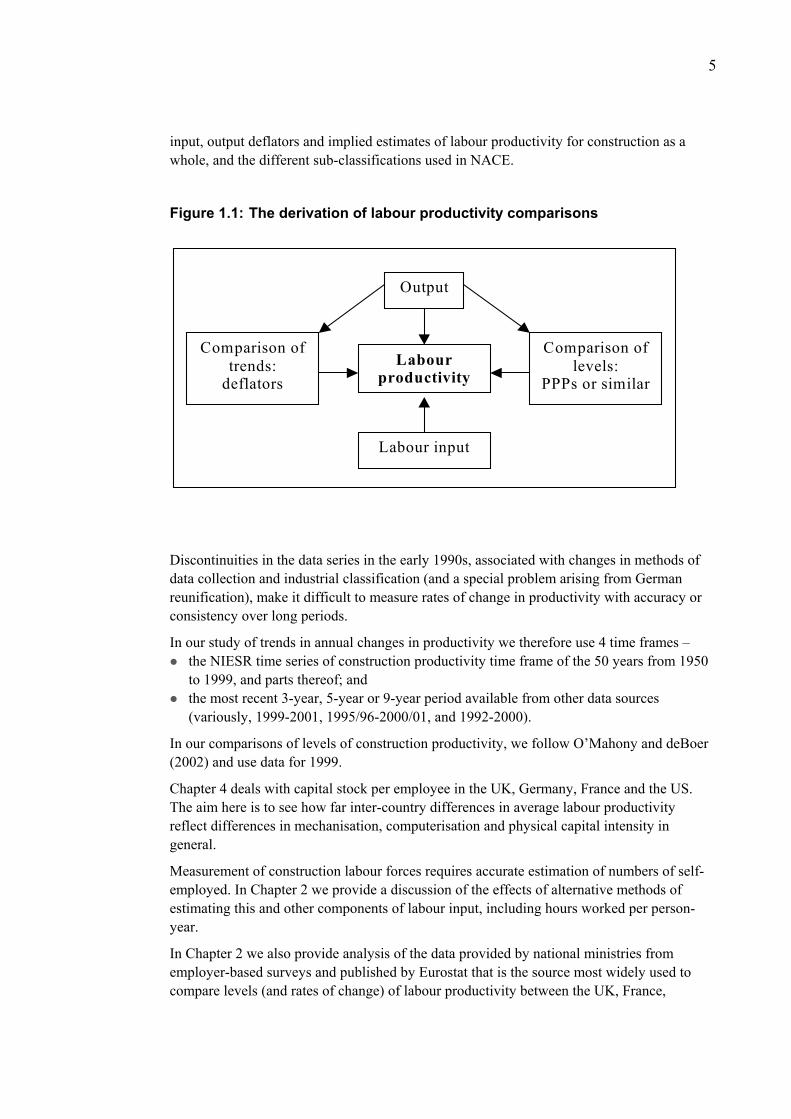
The basic shape of this research is shown in the flow chart given in Figure 1.1. It illustrates that labour productivity is a function of measures of output (usually value-added) and labour inputs (either numbers engaged in construction activities, numbers of jobs, total labour hours worked or the costs of employment). In order to compare trends over time appropriate deflators are required and in order to compare levels in different countries purchasing power parities are used rather than exchange rates.

Contents

In Chapter 2 we begin by examining, for construction, the findings, sources and methods of the main recent set of attempts to study international sectoral productivities; viz. the NIESR 2002 database, O’Mahony (1999) and O’Mahony and deBoer (2002). We do this by comparing productivity levels, rank orders and ratios in the UK, USA, France and Germany. This Chapter of the report uses both construction-product relative price levels and construction PPPs and whole-economy or GDP PPPs. We identify the 3-digit sub-sectors of construction for which comparative international data are available, and examine the extent to which particular sub-sectors are responsible for international differences in productivity in construction. Then in Chapter 3 we estimate rates of change in output, employment and labour productivity for construction as a whole and also by specialisation of firm in the UK, France and Germany. This part of the report uses annual changes in value-added, labour

5

input, output deflators and implied estimates of labour productivity for construction as a whole, and the different sub-classifications used in NACE.

Figure 1.1: The derivation of labour productivity comparisons

Output

Labour productivity

Comparison of trends:

deflators

Comparison of levels:

PPPs or similar

Labour input

Discontinuities in the data series in the early 1990s, associated with changes in methods of data collection and industrial classification (and a special problem arising from German reunification), make it difficult to measure rates of change in productivity with accuracy or consistency over long periods.

In our study of trends in annual changes in productivity we therefore use 4 time frames – the NIESR time series of construction productivity time frame of the 50 years from 1950 to 1999, and parts thereof; and

the most recent 3-year, 5-year or 9-year period available from other data sources (variously, 1999-2001, 1995/96-2000/01, and 1992-2000).

In our comparisons of levels of construction productivity, we follow O’Mahony and deBoer (2002) and use data for 1999.

Chapter 4 deals with capital stock per employee in the UK, Germany, France and the US. The aim here is to see how far inter-country differences in average labour productivity reflect differences in mechanisation, computerisation and physical capital intensity in general.

Measurement of construction labour forces requires accurate estimation of numbers of self-employed. In Chapter 2 we provide a discussion of the effects of alternative methods of estimating this and other components of labour input, including hours worked per person-year.

In Chapter 2 we also provide analysis of the data provided by national ministries from employer-based surveys and published by Eurostat that is the source most widely used to compare levels (and rates of change) of labour productivity between the UK, France,

6

Germany and all other member countries of the EU. We conclude that, so far as UK construction is concerned, this data is inappropriate for comparative use and has flaws that have led users to draw unsound and misleading conclusions.

In Chapter 3 our discussion of trends in productivity includes a special discussion of the US data, which appears to show a startling long run decline in US construction productivity, and explain the shortcomings of the US data.

In Chapter 5 we compare productivity in the construction industry with productivity in the motor vehicle industry. The aim is to use output and labour data for both new and repair and maintenance sub-sectors in both construction and motor vehicle industries. In Chapter 6 we summarise addressing the terms of reference. Finally in Chapter 7 we conclude with recommendations and a summary of our main findings.

Acknowledgements

Abby Sneade, DTI; Paul Thomas, DLC; Frances Pottier, DTI; Mary O’Mahony, NIESR; Chris Nicholls, ODPM; Geoff Mason, DTI; Christopher Moir, DTI

7

2 International comparison of levels of construction industry productivity

This chapter compares, for 1999, labour productivity, output, labour input, and unit labour costs in the UK, US, France and Germany. The purpose of this comparison is to show the relative productivity performance of the UK in the context of broadly similar and, indirectly, competitor economies.

Compared with the main internationally-traded sectors, productivity-level comparison for construction is both harder to do and, in some senses, less urgently required. It is less urgent because a construction productivity gap does not have the same direct impact, via comparative unit costs, on international trade competitiveness of the industry, and thus on construction output and GDP levels. It is more difficult to do because of exceptional difficulties of both output and input measurement, and problems of finding appropriate rates of conversion to common purchasing-power units are increased by the heterogeneity of construction output and complexity of national differences in output mix and quality.

Focus on labour productivity

It is preferable in principle to compare both labour (LP) and total factor-productivities (TFP), rather than only the former. However, not only does TFP estimation require the analyst to make a series of assumptions (about forms of the production function, growth theory and income distribution theory) not required for simple LP calculation; but also it encounters formidable additional problems in the measurement of capital and human capital inputs, neither of which have ‘natural’ units or are surveyed as thoroughly or accurately as is labour input (by US Current Population Survey and European Labour Force Survey).

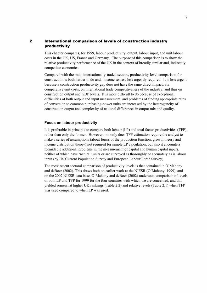
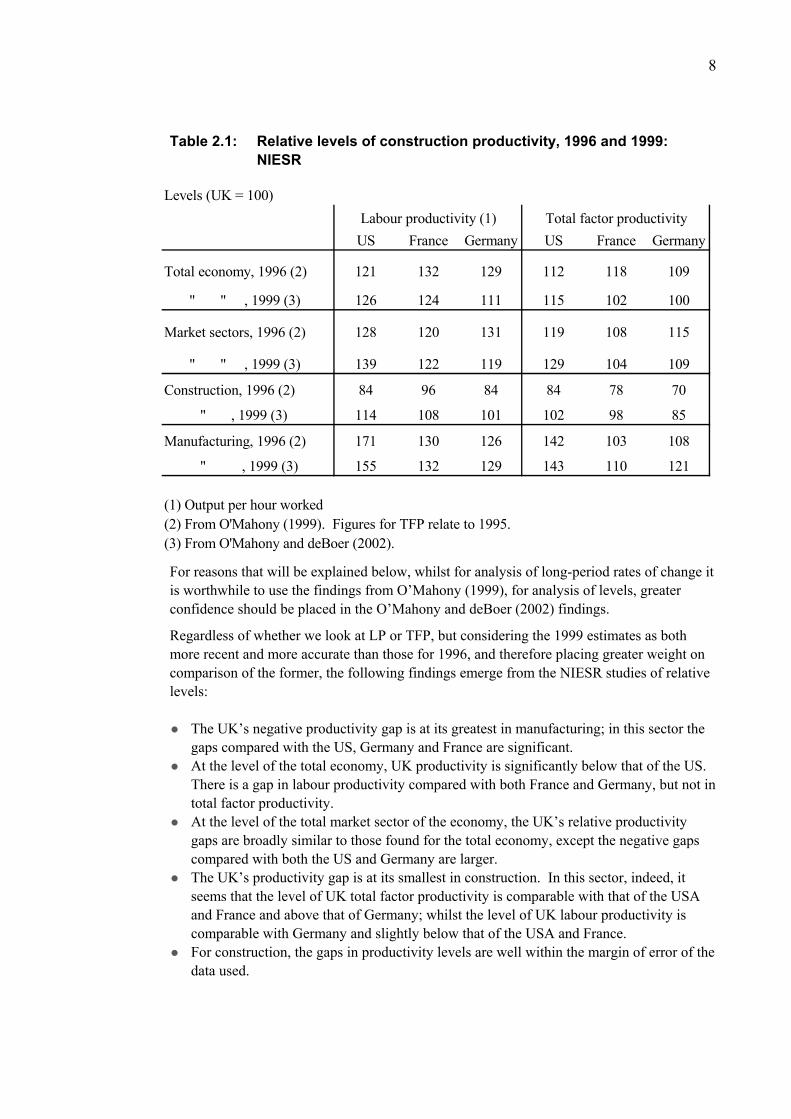
The most recent sectoral comparison of productivity levels is that contained in O’Mahony and deBoer (2002). This draws both on earlier work at the NIESR (O’Mahony, 1999), and on the 2002 NIESR data base. O’Mahony and deBoer (2002) undertook comparison of levels of both LP and TFP for 1999 for the four countries with which we are concerned, and this yielded somewhat higher UK rankings (Table 2.2) and relative levels (Table 2.1) when TFP was used compared to when LP was used.

8

Table 2.1: Relative levels of construction productivity, 1996 and 1999: NIESR

Levels (UK = 100)

US France Germany US France Germany

Total economy, 1996 (2) 121 132 129 112 118 109

" " , 1999 (3) 126 124 111 115 102 100

Market sectors, 1996 (2) 128 120 131 119 108 115

" " , 1999 (3) 139 122 119 129 104 109

Construction, 1996 (2) 84 96 84 84 78 70

" , 1999 (3) 114 108 101 102 98 85

Manufacturing, 1996 (2) 171 130 126 142 103 108

" , 1999 (3) 155 132 129 143 110 121

(1) Output per hour worked(2) From O'Mahony (1999). Figures for TFP relate to 1995.(3) From O'Mahony and deBoer (2002).

Labour productivity (1) Total factor productivity

For reasons that will be explained below, whilst for analysis of long-period rates of change it is worthwhile to use the findings from O’Mahony (1999), for analysis of levels, greater confidence should be placed in the O’Mahony and deBoer (2002) findings.

Regardless of whether we look at LP or TFP, but considering the 1999 estimates as both more recent and more accurate than those for 1996, and therefore placing greater weight on comparison of the former, the following findings emerge from the NIESR studies of relative levels:

The UK’s negative productivity gap is at its greatest in manufacturing; in this sector the gaps compared with the US, Germany and France are significant.

At the level of the total economy, UK productivity is significantly below that of the US. There is a gap in labour productivity compared with both France and Germany, but not in total factor productivity. At the level of the total market sector of the economy, the UK’s relative productivity gaps are broadly similar to those found for the total economy, except the negative gaps compared with both the US and Germany are larger. The UK’s productivity gap is at its smallest in construction. In this sector, indeed, it seems that the level of UK total factor productivity is comparable with that of the USA and France and above that of Germany; whilst the level of UK labour productivity is comparable with Germany and slightly below that of the USA and France. For construction, the gaps in productivity levels are well within the margin of error of the data used.

9

Construction is of course a labour-intensive industry in all these countries. Plant hire and leasing practices make its capital stock data particularly prone to error. Consequently, subsequent analyses in this report focus mainly on labour productivity. There is, however, a discussion of the relative capital stock and capital per worker in a later section (Chapter 4).

Table 2.2: Rank orders, construction productivity levels, 1996 and 1999: NIESR

Rank orders, construction productivity levels

(A) 1996LP TFP

UK 1 UK 1France 2 US 2

US 3= France 3Germany 3= Germany 4

(B) 1999LP TFP

US 1 US 1France 2 UK 2

UK 3 France 3Germany 4 Germany 4

Explanation of the differences between relative productivity levels, in O’Mahony (1999) and O’ Mahony and deBoer (2002)

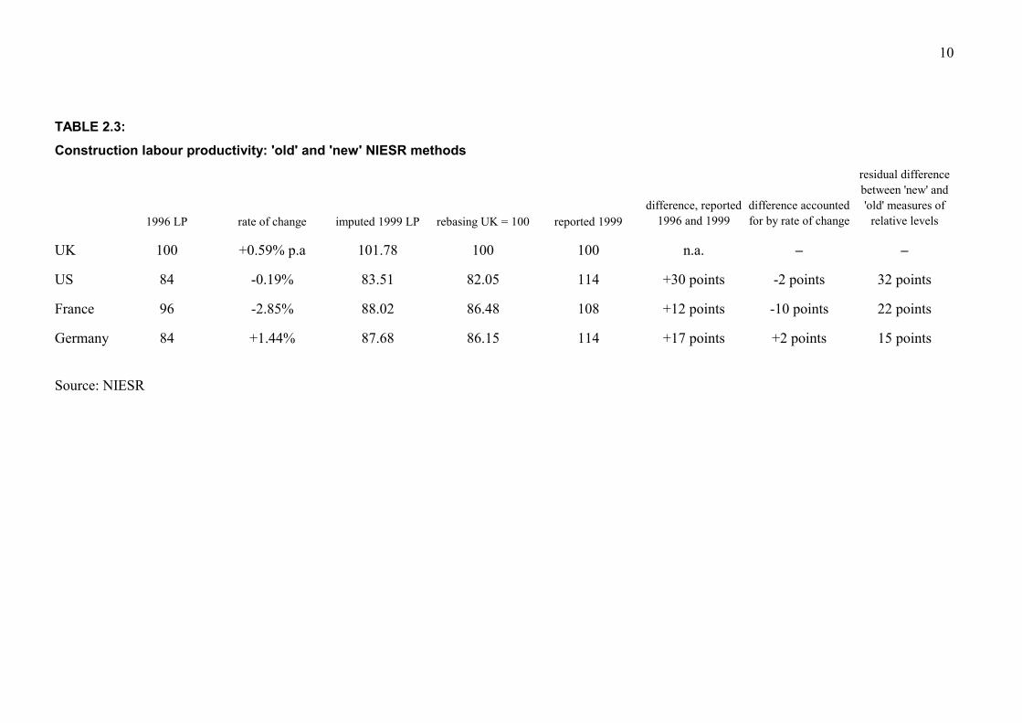
A part of the change might be attributable to differences in rates of productivity growth over the three-year period. However, in fact this accounts for only a negligible part, in one case (Germany), and yields a change in the ‘wrong’ direction in the other cases.

Taking the levels reported (O’Mahony, 1999) for 1996, and applying the annual rates of change reported for the period 1995-99 to those levels, we can derive imputed ‘old basis’ levels for 1999. These can then be compared to the ‘new basis’ reported levels for that year (O’Mahony and deBoer, 2002). See Table 2.3.

The last column of Table 2.3 gives an indication of the impact on estimation of relative construction productivity levels of the changes in the data sets and methods used by NIESR between O’Mahony (1999) and O’Mahony and deBoer (2002).

It is thus clear that these changes in methods require further comment and examination.

10

TABLE 2.3:

Construction labour productivity: 'old' and 'new' NIESR methods

1996 LP rate of change imputed 1999 LP rebasing UK = 100 reported 1999difference, reported

1996 and 1999difference accounted for by rate of change

residual difference between 'new' and 'old' measures of

relative levels

UK 100 +0.59% p.a 101.78 100 100 n.a. – –

US 84 -0.19% 83.51 82.05 114 +30 points -2 points 32 points

France 96 -2.85% 88.02 86.48 108 +12 points -10 points 22 points

Germany 84 +1.44% 87.68 86.15 114 +17 points +2 points 15 points

Source: NIESR

11

The biggest difference between the ‘old’ and ‘new’ NIESR methods as regards construction concerns differences in the approach taken to estimation of the sizes of the construction labour force, specifically its self-employed component.

Table 2.4: Estimates of size of UK construction labour force

Persons engaged (NIESR, 1999) and total jobs (Blue Book, 2000) in thousands

NIESR BB NIESR BB NIESR BB NIESR BB NIESR BBConstruction 1,189 1,729 1,226 1,738 1,269 1,750 1,600 2,053 -25.7% -15.8%Agriculture 529 546 524 548 528 583 571 621 -7.4% -12.1%Total economy 25,160 26,347 24,819 26,058 24,367 25,666 25,319 26,467 -0.6% 0.0%

Sources: O'Mahony (1999), Table B; ONS (2000), UK National Accounts, Table 2.5

%change1991-19961996 1995 1994 1991

For the total economy, the difference between NIESR (1999) ‘persons engaged’ and Blue Book ‘jobs’ is relatively small in all years (1,187,000 or +4.7% to ‘persons engaged’ in 1996; 1,148,000 or +4.5% to ‘persons engaged’ in 1991). This difference is readily mostly attributable to the minority of persons holding two jobs, and this is how it is interpreted in O’Mahony (1999).

However, for construction the difference is relatively large (540,000 or +45.4% to ‘persons engaged’ in 1996; 453,000 or +28.3% to ‘persons engaged’ in 1991), and is surely not to any significant degree attributable to construction workers holding two or more jobs at the same time. Instead, it requires an alternative explanation.

In principle:

(1) Persons engaged (NIESR, 1999) = employee jobs (firm-based surveys) – adjustment for employees with two jobs + estimated self employed (inter/extrapolation method)

(2) Total employed (BB) = employee jobs (firm-based surveys) + estimated self-employed jobs (Labour Force Survey)

Since O’Mahony (1999) uses the same employer surveys as the Blue Book to calculate employee jobs, most (though not all) of the difference between the NIESR and Blue Book figures for the total construction workforce must be attributable to differences in estimates of self-employment. For this the Blue Book uses the Labour Force Survey, whereas O’Mahony does not, but extrapolates from Population Census results for 1981 and 1991 using the intercensal 1981-91 rate of change in the share of self-employed in the total construction labour force.

This results, for the period 1991-96 for example, in significant discrepancies in the respective BB and NIESR figures for the sizes and rates of change in the construction labour force and thus in construction labour productivity.

12

Table 2.5: Construction output, labour force and productivity change

NIESR (1999)1991 1996 % change

Index of real output (1993 = 100) 105.5 104.5 -0.9%Number of persons engaged 1600 1189 -25.7%Rate of growth in output per person engaged (100) (133.3) +33.3%

Blue Book (2000)1991 1996 % change

GVA at 1995 base prices (1995 = 100) 102.3 101.5 -0.8%Total jobs 2053 1729 -15.8%Rate of growth in output per job (100) (117.8) +17.8%

Sources: O'Mahony (1999), Tables A and B; ONS (2000), UK National Accounts, Tables 2.4 and 2.5

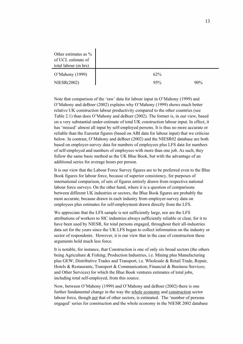
Table 2.6: Different estimates of UK labour input

Number of persons engaged (000s)

1991 1996 1999

O’Mahony (1999) 1,600 1,189

NIESR (2002) 2,053 1,729 1,767

Blue Book (2000), ‘jobs’

2,053 1,729 1,767

UCL (=LFS) 1,825 1,961

Average hours worked per person

O’Mahony (1999) 1,822 1,815

NIESR (2002) 1,914 1,907 1,935

UCL (=NIESR2002) 1,907 1,935

Total labour input (millions of hours)

O’Mahony (1999) 2,915 2,158

NIESR (2002 3,929 3,297 3,419

UCL (= LFS persons x NIESR02 hours

3,480 3,795

13

Other estimates as % of UCL estimate of total labour (m hrs)

O’Mahony (1999) 62%

NIESR(2002) 95% 90%

Note that comparison of the ‘raw’ data for labour input in O’Mahony (1999) and O’Mahony and deBoer (2002) explains why O’Mahony (1999) shows much better relative UK construction labour productivity compared to the other countries (see Table 2.1) than does O’Mahony and deBoer (2002). The former is, in our view, based on a very substantial under-estimate of total UK construction labour input. In effect, it has ‘missed’ almost all input by self-employed persons. It is thus no more accurate or reliable than the Eurostat figures (based on ABI data for labour input) that we criticise below. In contrast, O’Mahony and deBoer (2002) and the NIESR02 database are both based on employer-survey data for numbers of employees plus LFS data for numbers of self-employed and numbers of employees with more than one job. As such, they follow the same basic method as the UK Blue Book, but with the advantage of an additional series for average hours per person.

It is our view that the Labour Force Survey figures are to be preferred even to the Blue Book figures for labour force, because of superior consistency, for purposes of international comparison, of sets of figures entirely drawn from respective national labour force surveys. On the other hand, where it is a question of comparisons between different UK industries or sectors, the Blue Book figures are probably the most accurate, because drawn in each industry from employer-survey data on employees plus estimates for self-employment drawn directly from the LFS.

We appreciate that the LFS sample is not sufficiently large, nor are the LFS attributions of workers to SIC industries always sufficiently reliable or clear, for it to have been used by NIESR, for total persons engaged, throughout their all-industries data set for the years since the UK LFS began to collect information on the industry or sector of respondents. However, it is our view that in the case of construction these arguments hold much less force.

It is notable, for instance, that Construction is one of only six broad sectors (the others being Agriculture & Fishing; Production Industries, i.e. Mining plus Manufacturing plus GEW; Distributive Trades and Transport, i.e. Wholesale & Retail Trade, Repair, Hotels & Restaurants, Transport & Communication; Financial & Business Services; and Other Services) for which the Blue Book ventures estimates of total jobs, including total self-employed, from this source.

Now, between O’Mahony (1999) and O’Mahony and deBoer (2002) there is one further fundamental change in the way the whole economy and construction sector labour force, though not that of other sectors, is estimated. The ‘number of persons engaged’ series for construction and the whole economy in the NIESR 2002 database

14

(on which O’Mahony and deBoer 2002 is based) are identical, for the period 1991 to 1999, to the figures for ‘number of jobs’ given in the Blue Book, and taken, as far as self-employment jobs are concerned, directly from the LFS. Thus, O’Mahony has switched, at the level of the whole economy and for construction, from counting persons to counting jobs.

At the level of the construction sector, between O’Mahony (1999) and O’Mahony and deBoer (2002) the inter/extrapolation method (described below) for estimating self-employment has been abandoned, and replaced by use of LFS estimates. This accounts for almost all the differences between O’Mahony (1999) and O’Mahony and deBoer (2002) in the estimates for relative levels of UK construction productivity. Whereas the 1999 NIESR study found UK construction productivity levels to be somewhat higher than those of France, Germany and the US, the 2002 NIESR study found the reverse. Rather than treat these as two different but both valid attempts to estimate ‘actual’ relative construction productivity levels, we incline to relative confidence in the latter (2002) estimate.

Labour input was measured by both O’Mahony (1999) and O’Mahony and deBoer (2002) as ‘persons engaged’ and ‘number of hours’. For most of the period covered by O’Mahony (1999), the UK’s Census of Employment did not classify the self-employed to sector. Thus in O’Mahony (1999) ‘persons engaged’ in each sector comprised reported employees in employment (number of jobs, not persons) plus an estimate of the share of self-employment, based on the share of each sector’s self-employed as a proportion of total persons engaged in that sector as reported in the decennial Population Census.

Thus, between Population Census years, O’Mahony’s (1999) estimate for self-employment in a sector (say, construction) rises or falls in a set proportion to the rise or fall in the reported number of employees in employment in that sector. This proportion is derived by linear interpolation. Thus, suppose that the 1971 Census reported that out of every 100 persons engaged in construction, 20 were self-employed and that the 1981 Census reported that 30 out of every 100 were self-employed. By linear interpolation, the assumption is that in, say, 1976, 25% of the construction workforce would be self-employed. If reported employees in employment in construction in 1976 were X thousand, then total persons engaged, Y, would be estimated as X / (1–0.25) and total self-employed, S, as Y–X.

The overall effect is simply to average-out any change in the proportion of self-employed over a decade as if that change occurred smoothly, as a constant rate. Where, in reality, the changes in S/Y were sharp, discontinuous and reversed, this method introduces significant error into estimations of short-period rates of change in construction labour productivity, and some error into estimates of relative international levels.

Interpolation can obviously only be used to estimate self-employment backwards from the latest available population census. It is clear that estimates for years 1992-96 in O’Mahony (1999) must have been based on extrapolation (the latest Population Census cited as a source on pp. 43-44 is that for 1991). Its estimates for self-employment by sector for 1992-96 must be based on extrapolation of the linear rate of

15

change in the share of self-employed in sector workforces during the previous decade, 1981 to 1991.

This obviously introduced considerable probable error into these estimates. For a sector where self-employment is very important (construction, but also agriculture) it would imply that we should be circumspect in interpreting O’Mahony (1999) results for labour productivity levels and trends post-1991.

A sharp rise and then sharp fall in the proportion of self-employed in persons engaged in construction during the 1990s is reported in DTI’s series for Manpower (Construction Statistics Annual) and in the Labour Force Survey. This then explains the drop, between O’Mahony (1999) and O’Mahony and deBoer (2002) in NIESR’s measure of the UK’s construction labour productivity relative level.

By 2002, the NIESR dataset had switched to the use of Labour Force Survey data to measure self-employment in construction and number of persons with more than one job. The main difference between this and the Census of Employment is described in O’Mahony and deBoer (2002) thus: that the former counts persons whereas the latter counts jobs.

Now, whilst it is true that this is an important difference, it is by no means the only difference. O’Mahony notes one such difference thus: ‘In practice there are also differences in average annual hours worked measures from establishment and household surveys (i.e. between Census of Employment and Labour Force Surveys) which cannot be explained fully by the distinction between employment and jobs’ (O’Mahony and deBoer, 2002, p. 41).

The NIESR ‘old’ method is based on data from establishment surveys, supplemented by separate NSI estimates of ‘time lost’. It thus excludes unpaid overtime hours, and provides no direct measure of the hours worked by the self-employed. The NIESR ‘new’ method is still not based on LFS data for hours worked. We recommend: further international research, in association with NIESR, into the feasibility of using this LFS data as source for hours worked per person for the broad industry sectors (single-digit industry groups), including construction, for each of the countries (or at least for UK, France, Germany and USA, if not for Japan) in the NIESR dataset. Again, the advantage potentially would be greater international comparability of national data. In some countries, this would imply consideration of adding a question on ‘industry’ to the present household survey instrument. On some of the difficulties that would have to be overcome, see below.

Meager (1992) notes a further point, likely to affect measured self-employment. If self-employment data (in some countries) is derived from surveys of establishments or from tax or social insurance data, it will tend to reflect official definitions of who should count as self-employed. If it comes from the LFS, on the other hand, it will reflect workers’ self-perception of their employment status. The discrepancy will perhaps mainly concern working proprietors in small but incorporated business. Legally, these are employees. But in self-reporting many will surely be reported as self-employed.

16

Labour Force Survey as source of estimates for construction labour input

We concentrated our investigation into sources and methods for labour input data onto the European LFS and its close US equivalent, the Survey of Current Population, because this permits us to use closely comparable sources for all the four countries.

In each country the LFS covers “persons aged 16 and over, living in private households”. It is in each country based on a survey of households. It excludes persons living in ‘collective households’. For construction, the significance of this is that it excludes workers provided with temporary accommodation by employers at construction sites, or living in hostels or similar accommodation near to sites. However, if the permanent address of such workers is surveyed, it may be that other members of their private household respond on their behalf.

It uses common definitions, based on ILO recommendations. For our purposes, one key point is that it is supposed to use the respondent’s own assessment of their employment status, that is, whether they are an ‘employee’ or ‘self-employed’.

LFS in the UK

Before 1992, the UK LFS was an annual survey of some 80,000 addresses, with a response rate of 80-90%. Since 1992, it comprises a quarterly survey of five ‘waves’, each containing about 12,000 households. Thus there is a total of about 60,000 household-responses per annum (though panel construction of the survey means many of these households have responded more than once within the year).

These 60,000 ‘household units’ per annum yield some 138,000 responses for individuals per year.

Persons responding are a 1/300 sample of the estimated population of persons (it is not a sample of one in three hundred households) [0.33%]. The UK economically active population is about 29 million. Thus the ‘population sampling’ fraction is about 0.45% if each ‘response’ is counted separately, whether by the same respondent as others or not.

Unlike some other countries, it collects data on ‘industry’ in which respondent is economically active. This data is not used directly in producing figures for ‘employees by industry’ (this still comes from surveys of employers, in all industries), but it is used, together with responses to the self-employment question, to estimate the ‘self-employment by industry’ sub-totals to be added to the former to produce industry totals for ‘employment’ and for ‘jobs’. Sample size and thus numbers of respondents in each quarter is too small to permit this source to be used to produce estimates for each 2-digit SIC industry. However, it is used to produce estimates for single-digit industry groups, of which construction is one.

Those in employment include employees, the self-employed, those on government training schemes, family workers and those who did not state their employment status.

In 2000, 15% of all male and 7% of all female respondents reported themselves as ‘self-employed’. This converts to approximately 2.3 million self-employed men in the economically active population. Of those men, some 27% say they work in the

17

construction industry. This ‘grosses up’ to 620,000 male self-employed construction workers. The number of female self-employed construction workers is tiny by comparison (1% of 800,000) at 8,000.

There are an unknown number of non-EU nationals without UK work permits who are nevertheless working (illegally) in the UK. They are likely to be concentrated in labour-intensive and low-paid occupations. They are unlikely to be included in employers returns and most will also escape the LFS.

Analysis of results of the 2001 Population Census has led to some downward revisions in former LFS-based estimates of the size of the UK workforce (LFS grossing factors for particular sub-groups of the population were found to have become too large).

LFS in France

In France the LFS consists of a single annual survey of some 65,000 households, two-thirds of which are used for 2 consecutive years. This is a 1/300 (0.33%) sample of households – that is, there are around 20 million households in France.

Small internally homogeneous cluster areas are used, in the same basic manner as in the UK.

Each year, the survey includes a question on ‘employment status’ (whether self-employed) and industry in which respondent is economically active.

Presumably, this data on ‘industry’ can be used, as in the UK but unlike Germany, to produce estimates of the number of self-employed in each main industry group, of which construction would be one. We have not been able to establish whether or not any such adjustment is actually made to the French series for construction employment. It may be that the number of self-employed construction respondents in the French LFS is too small to permit a ‘grossing’ estimate for the construction industry on its own.

Data refer to March of each year.

Corrections to LFS estimates are made after data from each decennial population census becomes available. The latest available Census is used to create a system of weighting for the LFS for the following decade. The population census does not ask for ‘industry’ in which someone works. Thus it cannot be used to update or correct ‘industry’ weights, and thus no such weights are used in the LFS.

LFS in Germany

The German LFS is conducted once annually “together with the microcensus”. Most key LFS questions are integrated within the questionnaire of the microcensus. Thus respondents may not even be aware that they are contributing to the LFS. There is a special law regarding the Mikrozensus under which it is compulsory for a person to answer all questions in the microcensus if they are selected in its sample. It is hard to know what the effect of this compulsion element (absent elsewhere) might be. In France and the UK, non-response (in whole or in part) creates significant problems. Complete refusal to respond requires replacement within the sample, which in turn creates problems of discontinuity for ‘panels’. Partial non-response is dealt with in

18

UK by instructions to interviewers on some key questions not to move on until the question is answered. If no answer is forthcoming, the whole interview should then be discarded. This may encourage interviewers to ‘make up’ some responses. Again, in UK and France, people who, for whatever reason, dislike being objects of ‘official’ attention or supplying information to “the authorities” can simply refuse to participate, and thus will not be represented in LFS results. In Germany, compulsion may mean that everyone selected obeys, or it may mean that some persons go to great efforts to avoid being found.

The microcensus is a 1% annual sample survey covering all Census enumeration districts. Thus there is no geographical clustering. Some 45% (federal average) of households included in the microcensus are also asked (integrated) LFS questions. The remaining 55% are only asked microcensus questions. Some additional LFS questions are voluntary, and are asked on a separate form.

Thus 0.45% of German households complete LFS survey questionnaires each year.

Data refer to March of each year.

One compulsory question in the microcensus asks for citizenship as recorded in a person’s passport. It allows, however, self-declaration of citizenship by the respondent, without documentary support. Non-EU nationals without full rights to work in Germany may, if surveyed, therefore respond by claiming to be German (or another EU nationality), if they fear answers pass to the Immigration authorities. Likewise, ‘lump’ workers not paying German income taxes or social insurance may, even if EU citizens, try to avoid being ‘found’ or, if found, not to report their employment status accurately.

Other (non-LFS) data on employment in Germany comes from the various social insurance schemes. Though in principle compulsory and comprehensive, these are estimated to cover only about 80% of the economically active population. For those so covered, data is returned by employers to local social insurance offices, processed by them, and forwarded to the Federal Institute for Employment (BfA). This in turn supplies data to the Federal and Lander Statistical Offices.

This data set excludes: Employees working less than 50 days a year, or less than 15 hours a week.

All self-employed, because these are not eligible for the social insurance scheme. Foreign workers who are not participants in the social insurance scheme.

It is this social insurance data set that collects data on economic branch of employment, including industry.

Thus, German employment data originating from the social insurance schemes will understate the real size of the total workforce and, perhaps especially, the size of the construction industry workforce, since both foreign and self-employed workers are likely to be disproportionately present in construction.

Whilst aggregate estimates for employment in the whole economy can be adjusted using data from the German LFS, it would appear that industry-specific adjustments cannot be made from this source, other than by assumption.

19

Summary on LFS

It is far from being a perfect source. It suffers from some failure to capture migrant workers and workers in temporary accommodation. Its sample size can be too small to yield reliable estimates for ‘cells’ containing only a small fraction of the economically active population. Its self-definition approach makes it hard to reconcile results with those based on legal or fiscal or other official definitions. Nevertheless, it is far better to have it and be able to use it than not.

Its main potential industry-level uses are: As a cross-check on employer-survey-based estimates of employees in employment. This is especially useful in industries such as construction where a significant proportion of employment is by firms employing less than 20 persons. Such firms are usually either not surveyed at all in employer-based surveys, or surveyed at a very low sampling fraction and with reduced-scope questionnaires.

As the best and main source of industry-level data on all those falling outside the scope of such employer-based or social-insurance-based censuses; whether because they are self-employed, foreign, working illegally, or for some other reason. It is much better as a source for self-employment than for the other categories of worker excluded from the other sources of data. As the best source for hours worked per person (including self-employed persons).

Further research would be needed to establish whether or not present UK construction labour force estimates (employees from firm-based inquiries plus self-employed from the LFS) are consistent with those for France. It is however fairly clear that they cannot be consistent with those for Germany, where it would seem to be impossible at present for anyone to estimate self-employment by industry. This could be solved by inclusion of an ‘industry’ question in the German LFS, however.

At present estimates of construction productivity are mostly (leaving aside NIESR02) either ‘per person’ or ‘per job’, and thus not directly comparable with DTI and ONS recommended methodology for international comparisons of productivity (ICP). That methodology is set out in Harley and Jones (1998) who recommend, where the data is robust, use of ‘hours’ as the measure of labour input. There is a special problem of lack of robustness in construction industry ‘hours’ data. The data collected is from surveys of employers, and relates only to employees. The only feasible source of an ‘hours’ estimate for the self-employed would be from the LFS. However, what is required is ‘hours worked per year’ and there would be difficulties in inferring this with confidence from four relatively small, quarterly surveys asking about ‘the last week’. Also, “a study in Finland” (quoted in Richardson, 2001) “suggests that the self-employed…tend to over-estimate their hours worked”.

Conversion of national outputs into equivalents: PPPs

Both NIESR studies used the following basic method. Bilateral ratios of nominal output in the construction sector were converted by the ratios of the countries’ output prices. This approach was adopted because of the absence of any appropriate indicator of physical output quantity.

20

The heterogeneity of construction output (and absence of Bills of Quantities in other countries) made it impossible to compute and use ‘unit value ratios’ (the ratios of values of sales divided by quantities produced) and thus the price ratios for construction used to convert nominal output value added were based on purchasing power parities (the ratios of final expenditure prices for construction goods, i.e. built products, as estimated by OECD).

Because construction produces mainly final and not intermediate goods, the appropriate ratios are those of purchaser prices.

OECD provides PPPs (price ratios) for 150 categories of products over the whole economy. The price ratios for construction were based on PPPs for new buildings (and not for infrastructure, or for repair and maintenance work).

O’Mahony (1999) used OECD PPPs and price ratios for 1993, whilst O’Mahony and deBoer (2002) used 1996 PPPs.

Bilateral price ratios are turned into composite and transitive aggregate sector price ratios by weighting individual product PPPs by expenditure shares using the EKS multilateral weighting system. These weighted sector-specific price ratios were found to be broadly consistent with the PPPs used for the whole economies.

Relative reliability of manufacturing and construction national price ratios

It should be noted that, for manufacturing, O’Mahony (1999) did use unit value ratios (see above) to calculate relative national price levels and to convert nominal value added to a common equivalent, and thus to estimate relative productivity levels. Moreover, these unit value ratios were applied to data from manufacturing industries’ censuses of production rather than to data from national accounts. ‘The use of the census (of production) ensures that output and employment referred to the same firms, which was considered more reliable than the national accounts where output and employment are often derived from different sources.’ (O’Mahony, 1999, p. 38).

Query: Could this difference in source of the estimates for manufacturing from that for other sectors in part explain why the apparent differences in productivity levels are much greater in manufacturing than elsewhere?

Answer: It is possible that some part of the wider productivity gap found by O’Mahony (1999) for manufacturing than for most of the rest of the market sector may be accounted for by this difference in data source and method for comparing price levels. This seems worthy of further investigation, but lies outside the scope of this report.

21

Table 2.7: Purchasing power parities for construction and for all final expenditure (GDP) 1996 price levels

construction GDP constructionFrance 100 116 90Germany 126 122 108UK 74 91 84US 87 91 97

OECD total – – 103source: OECD (1996) pp. 142-5, Table A2

source: OECD (1999) pp. 118-21, Table 11

Table 2.7 shows, for 1996, firstly, the comparative price levels of all final expenditure (GDP) and final expenditure on construction, in each of the four countries being compared, and secondly, the ratio of relative construction prices to relative total final expenditure prices. Table 2.7 shows that UK relative purchasing power, and thus output valued on an internationally-comparable basis, was in 1996 generally higher than would be indicated by a simple comparison of national outputs converted at exchange rates to a common currency, and that this is particularly so for construction (price ratio = 74, compared to OECD average of 100).

Table 2.8: Purchasing power parities 1993 price levels

over

all

resi

dent

ial

build

ings

non-

resi

dent

ial

build

ings

civi

l en

gine

erin

g w

orks

GD

P

over

all

resi

dent

ial

build

ings

non-

resi

dent

ial

build

ings

civi

l en

gine

erin

g w

orks

France 89 94 99 71 103 93 94 104 77Germany 115 138 118 81 113 108 125 112 78UK 74 71 86 66 85 93 82 105 86US 84 88 87 77 89 98 98 103 93OECD total – – – – – 105 101 107 110

comparative dollar price levels of final expenditure on GDP

(OECD = 100)

relative price levels of final expenditure on GDP

(GDP = 100)

source: OECD, Purchasing Power Parities. GK Results 1993 , Vol.II,

source: OECD (1995) pp. 32-3, Table 1.6

Table 2.8 shows the same price ratios as Table 2.7, but for 1993. Comparing Tables 2.7 and 2.8, we see that, although the relative price ratios for UK total final expenditure changed between 1993 and 1996, this was not so for the construction

22

price ratio (a fall in nominal UK construction prices relative to other UK prices offsetting a rise in all UK prices relative to other countries).

Eurostat and OECD regularly (every 3 years) produce Purchasing Power Parities (PPPs) for construction outputs as part of wider surveys of price levels in EU and OECD member (and EU candidate) countries. Construction PPPs are derived from a survey based on a small panel of national experts pricing bills of quantities representing different types of construction work. The results are then weighted to represent the composition of national construction output.

Although the surveys and related work have been undertaken for the past twenty-five years, the methodology used and the results obtained are not particularly reliable. DLC have been involved as national experts since 1980 and as Eurostat survey co-ordinators since 2000. Work is currently in-hand to improve the quality of the surveys and to disseminate survey results, but it will be some time before reliable construction price level indicators are available.

On the other hand, PPPs are preferable to simple unadjusted exchange rates in making inter-country comparisons of price levels. It is our view, however, that general GDP PPPs (dominated by consumption goods and services) are preferable, for application to construction goods, to construction-specific PPPs, at least for the time being.

We would therefore recommend further ICP (international comparisons of productivity) research using NIESR and LFS data sets, sources and methods, but using general GDP and not sector-specific PPPs to convert construction output prices to a common unit of measurement.

The measurement of nominal value added of the construction industry

Two published sources exist for construction value added. One comprises national censuses of production, such as the UK’s ABI. The other is National Accounts value added, published after reconciling three sources of data: factor incomes data; aggregate final expenditure data; and output (production) data. The ability to subject production-inquiry-based data to cross-checks with expenditure, income and input-output data for other industries gives National Accounts industry value added estimates a considerable advantage in terms of likely accuracy.

Production-inquiries have varied both over time and between countries in their completeness of coverage and methods. Even where there have been improvements over time (as in the UK, with the replacement of the CoP by the ABI) these have the effect of introducing discontinuities into time series derived from this source. By comparison, National Accounts estimates of industry value added almost certainly have greater consistency through time.

Both sources face the problem of unrecorded output, and of accurate apportionment of final-demand into value added at each stage in the value chain (sequence of industries producing intermediate products).

All production-based inquiries begin by asking firms to report, firstly, their gross output, and then their purchases from other industries. They do not normally ask

23

directly for gross profit income. Instead this is imputed: gross value added is imputed by deducting purchases from gross output; then gross profits are imputed by deducting ‘compensation of employees’ from value added. The estimates of factor-shares in value added (income) derived in this way are therefore at some risk of error.

A further complication is that firms report, as their gross output, sales to all other firms whatsoever. This includes sales to other construction-industry firms (sales by subcontractors to main contractors). For the concept of gross output of an ‘industry’ it is necessary to ‘net-out’ or disregard such sales, because they do not cross the boundary of the industry.

Query : Would it be preferable, on the grounds that “The use of the census of production ensures that output and employment refer to the same firms, whereas in the national accounts output and employment are often derived from different sources”, to use data from the censuses of production for construction, rather than use National Accounts data for output and LFS data for employment?

Answer: Almost certainly it would not. The large number of construction firms not surveyed because employing less than 20 persons, incompleteness in the ABI (and other countries’ equivalents) database of construction firms, and the prevalence of self-employment, all mean that National Accounts data is almost certainly more reliable than Census of Production (ABI) data as a basis for measuring both construction employment and output. The unreliability of the ABI data for UK construction is discussed more fully in the following section of this report.

Productivity: the problems with the UK Eurostat data on value added and labour input

In this study we had hoped to use NewCronos Eurostat data from national Censuses of Production (equivalent to UK’s former Census of Production and Construction and new ABI) to compare: levels and rates of change in value added, turnover, numbers employed and employment costs, both for whole construction industries and across sub-sectors of the UK, French and German industries.

Unfortunately, examination of the data revealed major and unexplained ‘jumps’ for the UK, between 1996 and 1999 (in the case of data for enterprises employing 20+, i.e. those actually surveyed) and between 1995 and 1999 (in the case of data for all enterprises).

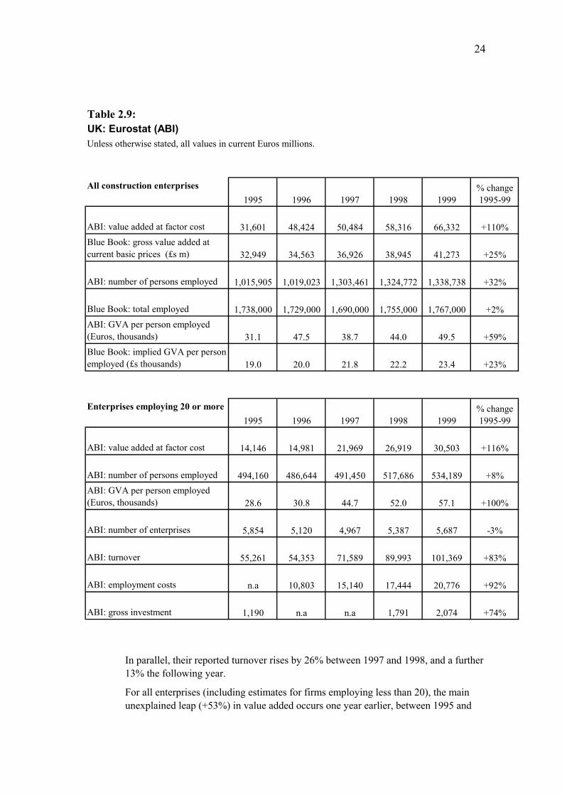
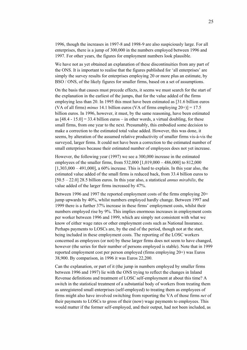
Table 2.9 shows the problem. For enterprises actually surveyed (employing 20+) there is an unexplained ‘leap’ upwards in value added of 47% between 1996 and 1997. This is not matched by any increase in the corresponding numbers of firms, or their numbers of employees, though there is also a (lesser) reported leap in their turnover of +32%. Naturally enough, this yields an apparent jump upward in the labour productivity of these firms. There is then a further increase of 23% in their value added between 1997 and 1998, and a further 13% increase the following year.

24

Table 2.9:UK: Eurostat (ABI)Unless otherwise stated, all values in current Euros millions.

All construction enterprises1995 1996 1997 1998 1999

ABI: value added at factor cost 31,601 48,424 50,484 58,316 66,332 +110%Blue Book: gross value added at current basic prices (£s m) 32,949 34,563 36,926 38,945 41,273 +25%

ABI: number of persons employed 1,015,905 1,019,023 1,303,461 1,324,772 1,338,738 +32%

Blue Book: total employed 1,738,000 1,729,000 1,690,000 1,755,000 1,767,000 +2%ABI: GVA per person employed (Euros, thousands) 31.1 47.5 38.7 44.0 49.5 +59%Blue Book: implied GVA per person employed (£s thousands) 19.0 20.0 21.8 22.2 23.4 +23%

Enterprises employing 20 or more1995 1996 1997 1998 1999

ABI: value added at factor cost 14,146 14,981 21,969 26,919 30,503 +116%

ABI: number of persons employed 494,160 486,644 491,450 517,686 534,189 +8%ABI: GVA per person employed (Euros, thousands) 28.6 30.8 44.7 52.0 57.1 +100%

ABI: number of enterprises 5,854 5,120 4,967 5,387 5,687 -3%

ABI: turnover 55,261 54,353 71,589 89,993 101,369 +83%

ABI: employment costs n.a 10,803 15,140 17,444 20,776 +92%

ABI: gross investment 1,190 n.a n.a 1,791 2,074 +74%

% change 1995-99

% change 1995-99

In parallel, their reported turnover rises by 26% between 1997 and 1998, and a further 13% the following year.

For all enterprises (including estimates for firms employing less than 20), the main unexplained leap (+53%) in value added occurs one year earlier, between 1995 and

25

1996, though the increases in 1997-8 and 1998-9 are also suspiciously large. For all enterprises, there is a jump of 300,000 in the numbers employed between 1996 and 1997. For other years, the figures for employment numbers look plausible.

We have not as yet obtained an explanation of these discontinuities from any part of the ONS. It is important to realise that the figures published for ‘all enterprises’ are simply the survey results for enterprises employing 20 or more plus an estimate, by BSO / ONS, of the likely figures for smaller firms, based on a set of assumptions.

On the basis that causes must precede effects, it seems we must search for the start of the explanation in the earliest of the jumps, that for the value added of the firms employing less than 20. In 1995 this must have been estimated as [31.6 billion euros (VA of all firms) minus 14.1 billion euros (VA of firms employing 20+)] = 17.5 billion euros. In 1996, however, it must, by the same reasoning, have been estimated as [48.4 - 15.0] = 33.4 billion euros – in other words, a virtual doubling, for these small firms, from one year to the next. Presumably, this embodied some decision to make a correction to the estimated total value added. However, this was done, it seems, by alteration of the assumed relative productivity of smaller firms vis-à-vis the surveyed, larger firms. It could not have been a correction to the estimated number of small enterprises because their estimated number of employees does not yet increase.

However, the following year (1997) we see a 300,000 increase in the estimated employees of the smaller firms, from 532,000 [1,019,000 – 486,000] to 812,000 [1,303,000 – 491,000], a 60% increase. This is hard to explain. In this year also, the estimated value added of the small firms is reduced back, from 33.4 billion euros to [50.5 – 22.0] 28.5 billion euros. In this year also, a statistical annus mirabilis, the value added of the larger firms increased by 47%.

Between 1996 and 1997 the reported employment costs of the firms employing 20+ jump upwards by 40%, whilst numbers employed hardly change. Between 1997 and 1999 there is a further 37% increase in these firms’ employment costs, whilst their numbers employed rise by 9%. This implies enormous increases in employment costs per worker between 1996 and 1999, which are simply not consistent with what we know of either wage rates or other employment costs such as National Insurance. Perhaps payments to LOSCs are, by the end of the period, though not at the start, being included in these employment costs. The reporting of the LOSC workers concerned as employees (or not) by these larger firms does not seem to have changed, however (the series for their number of persons employed is stable). Note that in 1999 reported employment cost per person employed (firms employing 20+) was Euros 38,900. By comparison, in 1996 it was Euros 22,200.

Can the explanation, or part of it (the jump in numbers employed by smaller firms between 1996 and 1997) lie with the ONS trying to reflect the changes in Inland Revenue definitions and treatment of LOSC self-employment at about this time? A switch in the statistical treatment of a substantial body of workers from treating them as unregistered small enterprises (self-employed) to treating them as employees of firms might also have involved switching from reporting the VA of those firms net of their payments to LOSCs to gross of their (now) wage payments to employees. This would matter if the former self-employed, and their output, had not been included, as

26

small enterprises, in the pre-1996 COP estimates of small firms’ output and employment.

On the other hand, taken at face value, the series imply that productivity in small (< 20) enterprises was: in 1995, higher (at €33,500) than in those employing 20+ (€28,600); in 1996, more than double that of larger firms (€62,800 c.f. €30,800); but substantially below that of the larger firms in 1997, 1998 and 1999. By 1999 this firm-size implied productivity differential stands at €57,000 (larger firms) to €44,500 (smaller firms). The direction and size of this differential at the end of the period are plausible on grounds of economic theory, whereas the differential at the start of the period is not so easy to explain.

We hesitate to suggest an even simpler explanation for some of the discrepancy between levels of value added reported in Eurostat and those in the original ABI. Is it possible that the Eurostat figures for 1995 value added are in fact in £s sterling and not, as of course they purport to be, in Euros?

However that may be, unexplained discontinuities such as these necessarily cause the user to lose confidence in the value of the data. If it was accurate up to 1995, then it is hard to see how it can also be accurate for the period 1995-99. If on the other hand, by 1999 it had become broadly accurate, then it must have been inaccurate for all earlier years. It is of course possible that it was inaccurate, but in different ways, both ‘before’ and ‘after’ these adjustments or jumps.

In contrast, the NewCronos COP data for the other EU construction industries looks plausible and ‘well-behaved’ as time series.

However, comparison of ABI data obtained directly from ONS/BSO, measured in £s, with the ABI data reported by Eurostat NewCronos, measured in €s, reveals that the former data set does not suffer from all of the problems of the latter. Therefore, in what follows we have to choose, at each point, between accuracy (original ONS data in £; only available for UK) and comparability (Eurostat data, with its known inaccuracies for the UK). Naturally, the consequence is that we are unable to use the data with confidence to make comparisons with France and Germany.

It is important that the problems affecting the Eurostat data for the UK be noted by the relevant UK government bodies, and that an effort be made, either by them or by Eurostat, to go back to the original UK CoP data (in £s) and recompute their conversion into Euros, for each sub-sector of construction and for each year from 1995 to the present. Pending this, the affected Eurostat data should be withdrawn from the NewCronos database. Unless this is done, other researchers and analysts may take the Eurostat data for the UK for 1995 to 2001 at face value, and draw seriously erroneous conclusions as a result.

Let the user beware

To illustrate this point, in the following section we show the apparent results if one takes Eurostat NewCronos Census of Production (ABI and equivalent) data for gross value-added at basic prices per head at ‘face value’ as a measure of productivity.

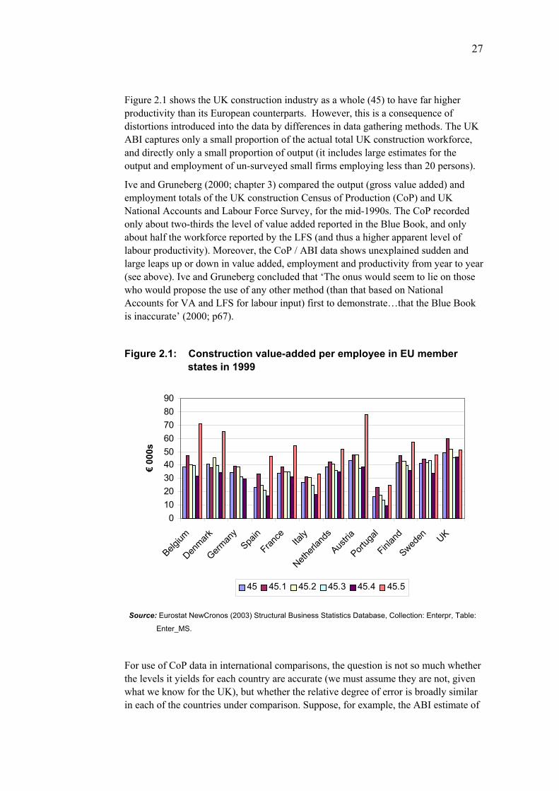
27

Figure 2.1 shows the UK construction industry as a whole (45) to have far higher productivity than its European counterparts. However, this is a consequence of distortions introduced into the data by differences in data gathering methods. The UK ABI captures only a small proportion of the actual total UK construction workforce, and directly only a small proportion of output (it includes large estimates for the output and employment of un-surveyed small firms employing less than 20 persons).

Ive and Gruneberg (2000; chapter 3) compared the output (gross value added) and employment totals of the UK construction Census of Production (CoP) and UK National Accounts and Labour Force Survey, for the mid-1990s. The CoP recorded only about two-thirds the level of value added reported in the Blue Book, and only about half the workforce reported by the LFS (and thus a higher apparent level of labour productivity). Moreover, the CoP / ABI data shows unexplained sudden and large leaps up or down in value added, employment and productivity from year to year (see above). Ive and Gruneberg concluded that ‘The onus would seem to lie on those who would propose the use of any other method (than that based on National Accounts for VA and LFS for labour input) first to demonstrate…that the Blue Book is inaccurate’ (2000; p67).

Figure 2.1: Construction value-added per employee in EU member states in 1999

0102030405060708090

Belgium

Denmark

German

ySpa

in

France Ita

ly

Netherl

ands

Austria

Portug

al

Finlan

d

Sweden UK

€ 00

0s

45 45.1 45.2 45.3 45.4 45.5

Source: Eurostat NewCronos (2003) Structural Business Statistics Database, Collection: Enterpr, Table:

Enter_MS.

For use of CoP data in international comparisons, the question is not so much whether the levels it yields for each country are accurate (we must assume they are not, given what we know for the UK), but whether the relative degree of error is broadly similar in each of the countries under comparison. Suppose, for example, the ABI estimate of

28

UK construction labour productivity is of the order of 30% too high. This does not matter, for a study of relative levels, if the Eurostat estimates for each other country also err in the same direction and by the same proportion. However, given the profound differences in industry structures and methods of data collection used in the CoPs, this would be an heroic assumption.

Figure 2.2 shows another misleading indicator of the relative position of UK value-added to labour. Unlike Fig. 2.1, it does not depend on exchange rates or PPPs for the comparison. Figure 2.2 shows the reported ratios of value-added to costs of employment. This is the inverse of the share of labour in value added. Thus a labour share of 76%, (the UK share for 1999, in NIESR02) would imply a ratio of 1.3 in VA per unit of employment costs. However, Figure 2.2 shows a much higher ratio, over 1.8. In Figure 2.2 the ratio of value-added to UK employment costs was slightly higher (i.e. the implied labour share in VA and unit labour cost was lower) than in several other countries including France, the Netherlands and Denmark.

Figure 2.2: Construction value-added per €1 of employment costs in EU member states in 1999

0.0

0.5

1.0

1.5

2.0

2.5

3.0

3.5

Belgium

Denmark

German

ySpa

in

France Ita

ly

Netherl

ands

Austria

Portug

al

Finlan

d

Sweden UK

€

45 45.1 45.2 45.3 45.4 45.5

Source: Eurostat NewCronos (2003) Structural Business Statistics Database, Collection: Enterpr, Table: Enter_MS.

This, of course, is because employment income (especially in the UK) is being underestimated, because of the exclusion of the ‘labour’ element in the mixed incomes of the self-employed (only a minority of whom are working proprietors, the remainder being LOSC workers).

The relationship between reported value-added per head and the ratio of VA to employment costs is shown in Figure 2.3. A linear regression shows a slight tendency for the value-added over employment costs to decline (i.e. for unit labour costs to increase) as value-added per employee increases. This appears to support the notion

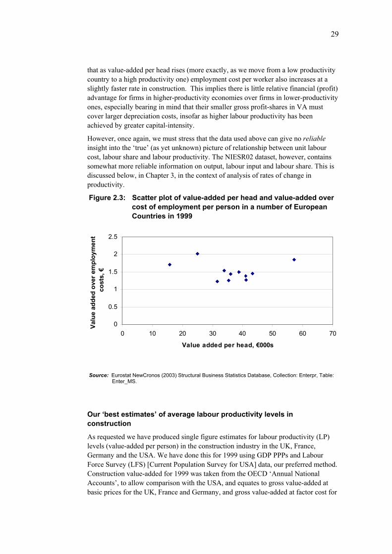
29

that as value-added per head rises (more exactly, as we move from a low productivity country to a high productivity one) employment cost per worker also increases at a slightly faster rate in construction. This implies there is little relative financial (profit) advantage for firms in higher-productivity economies over firms in lower-productivity ones, especially bearing in mind that their smaller gross profit-shares in VA must cover larger depreciation costs, insofar as higher labour productivity has been achieved by greater capital-intensity.

However, once again, we must stress that the data used above can give no reliable insight into the ‘true’ (as yet unknown) picture of relationship between unit labour cost, labour share and labour productivity. The NIESR02 dataset, however, contains somewhat more reliable information on output, labour input and labour share. This is discussed below, in Chapter 3, in the context of analysis of rates of change in productivity.

Figure 2.3: Scatter plot of value-added per head and value-added over cost of employment per person in a number of European Countries in 1999

0

0.5

1

1.5

2

2.5

0 10 20 30 40 50 60 70

Value added per head, €000s

Valu

e ad

ded

over

em

ploy

men

t co

sts,

€

Source: Eurostat NewCronos (2003) Structural Business Statistics Database, Collection: Enterpr, Table:

Enter_MS.

Our ‘best estimates’ of average labour productivity levels in construction

As requested we have produced single figure estimates for labour productivity (LP) levels (value-added per person) in the construction industry in the UK, France, Germany and the USA. We have done this for 1999 using GDP PPPs and Labour Force Survey (LFS) [Current Population Survey for USA] data, our preferred method. Construction value-added for 1999 was taken from the OECD ‘Annual National Accounts’, to allow comparison with the USA, and equates to gross value-added at basic prices for the UK, France and Germany, and gross value-added at factor cost for

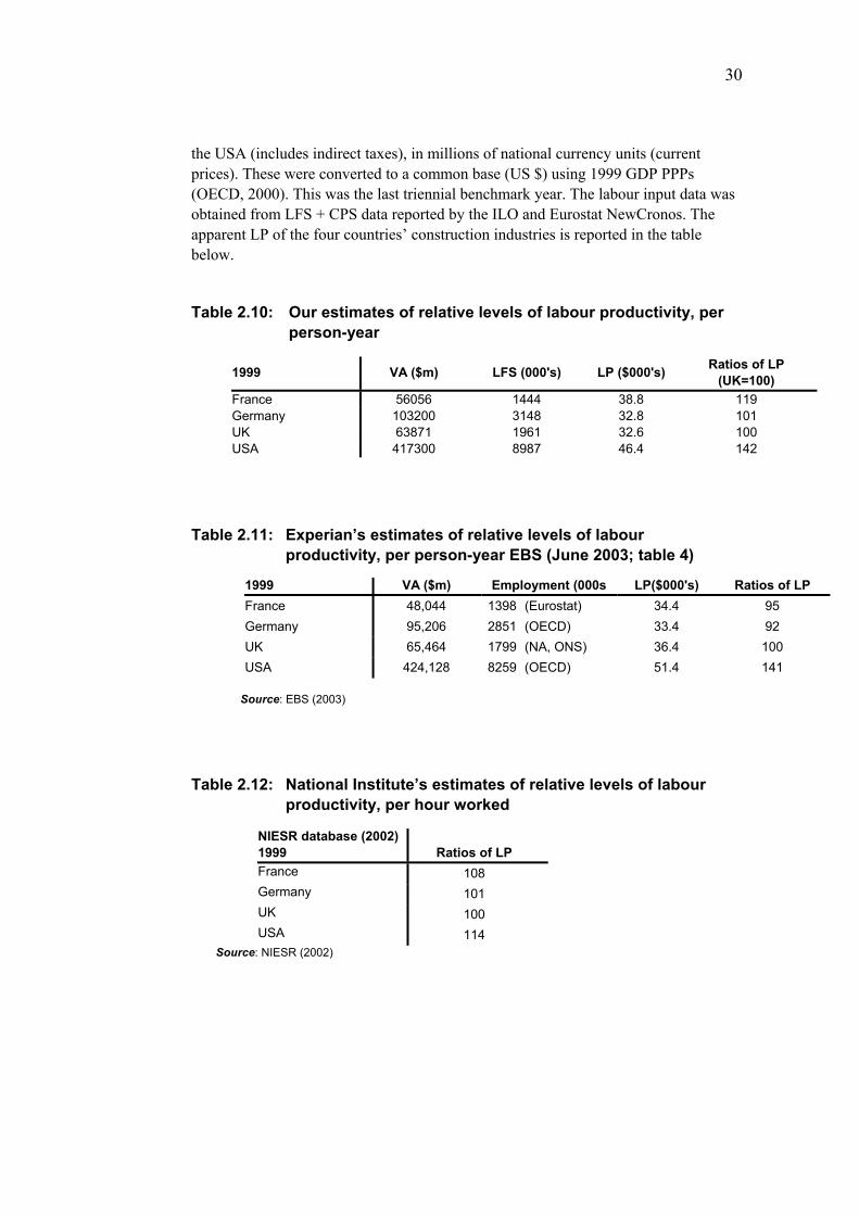
30

the USA (includes indirect taxes), in millions of national currency units (current prices). These were converted to a common base (US $) using 1999 GDP PPPs (OECD, 2000). This was the last triennial benchmark year. The labour input data was obtained from LFS + CPS data reported by the ILO and Eurostat NewCronos. The apparent LP of the four countries’ construction industries is reported in the table below.

Table 2.10: Our estimates of relative levels of labour productivity, per person-year

1999 VA ($m) LFS (000's) LP ($000's) Ratios of LP (UK=100)

France 56056 1444 38.8 119 Germany 103200 3148 32.8 101 UK 63871 1961 32.6 100 USA 417300 8987 46.4 142

Table 2.11: Experian’s estimates of relative levels of labour productivity, per person-year EBS (June 2003; table 4)

1999 VA ($m) Employment (000s LP($000's) Ratios of LP France 48,044 1398 (Eurostat) 34.4 95 Germany 95,206 2851 (OECD) 33.4 92 UK 65,464 1799 (NA, ONS) 36.4 100 USA 424,128 8259 (OECD) 51.4 141

Source: EBS (2003)

Table 2.12: National Institute’s estimates of relative levels of labour productivity, per hour worked

NIESR database (2002) 1999

Ratios of LP

France 108 Germany 101 UK 100 USA 114

Source: NIESR (2002)

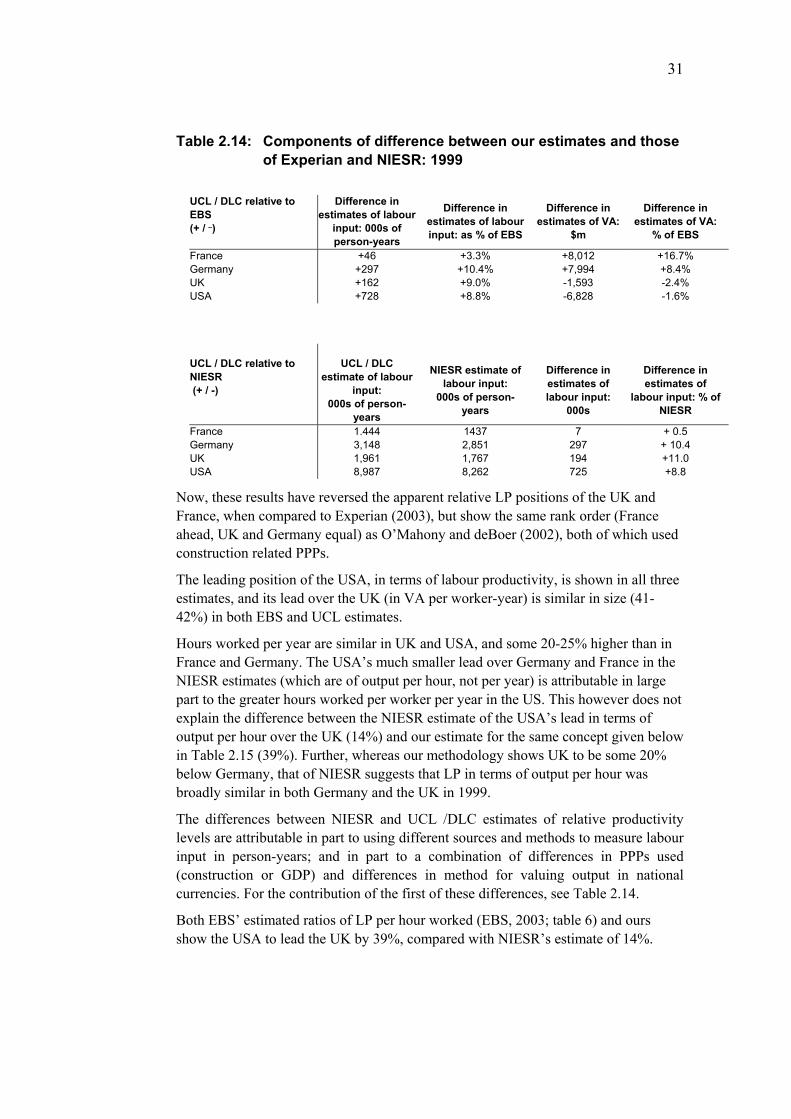
31

Table 2.14: Components of difference between our estimates and those of Experian and NIESR: 1999

UCL / DLC relative to EBS (+ / _)

Difference in estimates of labour

input: 000s of person-years

Difference in estimates of labour input: as % of EBS

Difference in estimates of VA:

$m

Difference in estimates of VA:

% of EBS

France +46 +3.3% +8,012 +16.7% Germany +297 +10.4% +7,994 +8.4% UK +162 +9.0% -1,593 -2.4% USA +728 +8.8% -6,828 -1.6% UCL / DLC relative to NIESR (+ / -)

UCL / DLC

estimate of labour input:

000s of person-years

NIESR estimate of

labour input: 000s of person-

years

Difference in estimates of labour input:

000s

Difference in estimates of

labour input: % of NIESR

France 1.444 1437 7 + 0.5 Germany 3,148 2,851 297 + 10.4 UK 1,961 1,767 194 +11.0 USA 8,987 8,262 725 +8.8

Now, these results have reversed the apparent relative LP positions of the UK and France, when compared to Experian (2003), but show the same rank order (France ahead, UK and Germany equal) as O’Mahony and deBoer (2002), both of which used construction related PPPs.

The leading position of the USA, in terms of labour productivity, is shown in all three estimates, and its lead over the UK (in VA per worker-year) is similar in size (41-42%) in both EBS and UCL estimates.

Hours worked per year are similar in UK and USA, and some 20-25% higher than in France and Germany. The USA’s much smaller lead over Germany and France in the NIESR estimates (which are of output per hour, not per year) is attributable in large part to the greater hours worked per worker per year in the US. This however does not explain the difference between the NIESR estimate of the USA’s lead in terms of output per hour over the UK (14%) and our estimate for the same concept given below in Table 2.15 (39%). Further, whereas our methodology shows UK to be some 20% below Germany, that of NIESR suggests that LP in terms of output per hour was broadly similar in both Germany and the UK in 1999.

The differences between NIESR and UCL /DLC estimates of relative productivity levels are attributable in part to using different sources and methods to measure labour input in person-years; and in part to a combination of differences in PPPs used (construction or GDP) and differences in method for valuing output in national currencies. For the contribution of the first of these differences, see Table 2.14.

Both EBS’ estimated ratios of LP per hour worked (EBS, 2003; table 6) and ours show the USA to lead the UK by 39%, compared with NIESR’s estimate of 14%.

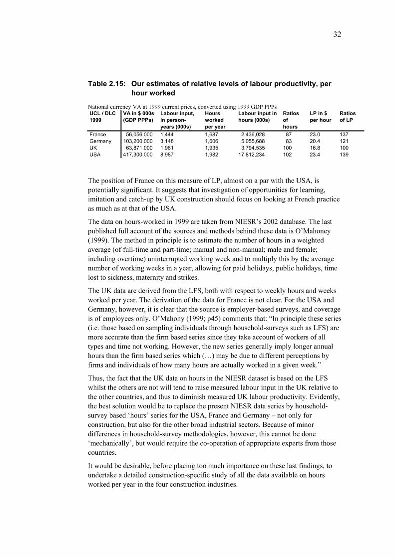
32

Table 2.15: Our estimates of relative levels of labour productivity, per hour worked

National currency VA at 1999 current prices, converted using 1999 GDP PPPs UCL / DLC 1999

VA in $ 000s (GDP PPPs)

Labour input, in person-years (000s)

Hours worked per year

Labour input in hours (000s)

Ratios of hours

LP in $ per hour

Ratios of LP

France 56,056,000 1,444 1,687 2,436,028 87 23.0 137 Germany 103,200,000 3,148 1,606 5,055,688 83 20.4 121 UK 63,871,000 1,961 1,935 3,794,535 100 16.8 100 USA 417,300,000 8,987 1,982 17,812,234 102 23.4 139

The position of France on this measure of LP, almost on a par with the USA, is potentially significant. It suggests that investigation of opportunities for learning, imitation and catch-up by UK construction should focus on looking at French practice as much as at that of the USA.

The data on hours-worked in 1999 are taken from NIESR’s 2002 database. The last published full account of the sources and methods behind these data is O’Mahoney (1999). The method in principle is to estimate the number of hours in a weighted average (of full-time and part-time; manual and non-manual; male and female; including overtime) uninterrupted working week and to multiply this by the average number of working weeks in a year, allowing for paid holidays, public holidays, time lost to sickness, maternity and strikes.

The UK data are derived from the LFS, both with respect to weekly hours and weeks worked per year. The derivation of the data for France is not clear. For the USA and Germany, however, it is clear that the source is employer-based surveys, and coverage is of employees only. O’Mahony (1999; p45) comments that: “In principle these series (i.e. those based on sampling individuals through household-surveys such as LFS) are more accurate than the firm based series since they take account of workers of all types and time not working. However, the new series generally imply longer annual hours than the firm based series which (…) may be due to different perceptions by firms and individuals of how many hours are actually worked in a given week.”

Thus, the fact that the UK data on hours in the NIESR dataset is based on the LFS whilst the others are not will tend to raise measured labour input in the UK relative to the other countries, and thus to diminish measured UK labour productivity. Evidently, the best solution would be to replace the present NIESR data series by household-survey based ‘hours’ series for the USA, France and Germany – not only for construction, but also for the other broad industrial sectors. Because of minor differences in household-survey methodologies, however, this cannot be done ‘mechanically’, but would require the co-operation of appropriate experts from those countries.

It would be desirable, before placing too much importance on these last findings, to undertake a detailed construction-specific study of all the data available on hours worked per year in the four construction industries.

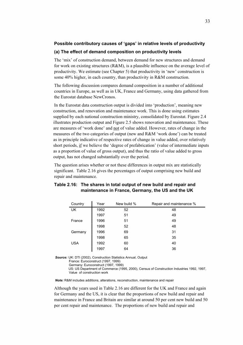
33

Possible contributory causes of ‘gaps’ in relative levels of productivity

(a) The effect of demand composition on productivity levels

The ‘mix’ of construction demand, between demand for new structures and demand for work on existing structures (R&M), is a plausible influence on the average level of productivity. We estimate (see Chapter 5) that productivity in ‘new’ construction is some 40% higher, in each country, than productivity in R&M construction.

The following discussion compares demand composition in a number of additional countries in Europe, as well as in UK, France and Germany, using data gathered from the Eurostat database NewCronos.

In the Eurostat data construction output is divided into ‘production’, meaning new construction, and renovation and maintenance work. This is done using estimates supplied by each national construction ministry, consolidated by Eurostat. Figure 2.4 illustrates production output and Figure 2.5 shows renovation and maintenance. These are measures of ‘work done’ and not of value added. However, rates of change in the measures of the two categories of output (new and R&M ‘work done’) can be treated as in principle indicative of respective rates of change in value added, over relatively short periods, if we believe the ‘degree of prefabrication’ (value of intermediate inputs as a proportion of value of gross output), and thus the ratio of value added to gross output, has not changed substantially over the period.

The question arises whether or not these differences in output mix are statistically significant. Table 2.16 gives the percentages of output comprising new build and repair and maintenance.

Table 2.16: The shares in total output of new build and repair and maintenance in France, Germany, the US and the UK

Country Year New build % Repair and maintenance % UK 1992 52 48 1997 51 49 France 1996 51 49 1998 52 48 Germany 1996 69 31 1998 65 35 USA 1992 60 40 1997 64 36

Source: UK: DTI (2002), Construction Statistics Annual, Output

France: Euroconstruct (1997, 1999) Germany: Euroconstruct (1997, 1999)

US: US Department of Commerce (1995, 2000), Census of Construction Industries 1992, 1997, Value of construction work

Note: R&M includes additions, alterations, reconstruction, maintenance and repair

Although the years used in Table 2.16 are different for the UK and France and again for Germany and the US, it is clear that the proportions of new build and repair and maintenance in France and Britain are similar at around 50 per cent new build and 50 per cent repair and maintenance. The proportions of new build and repair and

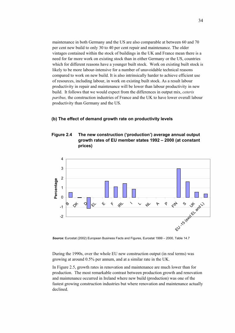
34

maintenance in both Germany and the US are also comparable at between 60 and 70 per cent new build to only 30 to 40 per cent repair and maintenance. The older vintages contained within the stock of buildings in the UK and France mean there is a need for far more work on existing stock than in either Germany or the US, countries which for different reasons have a younger built stock. Work on existing built stock is likely to be more labour-intensive for a number of unavoidable technical reasons compared to work on new build. It is also intrinsically harder to achieve efficient use of resources, including labour, in work on existing built stock. As a result labour productivity in repair and maintenance will be lower than labour productivity in new build. It follows that we would expect from the differences in output mix, ceteris paribus, the construction industries of France and the UK to have lower overall labour productivity than Germany and the US.

(b) The effect of demand growth rate on productivity levels

Figure 2.4 The new construction (‘production’) average annual output growth rates of EU member states 1992 – 2000 (at constant prices)

-2

-1

0

1

2

3

4

B DK D EL E F IRL I L NL A P FIN S UK

EU -15 (

excl

EL and

L)

Perc

enta

ge

Source: Eurostat (2002) European Business Facts and Figures, Eurostat 1999 – 2000, Table 14.7

During the 1990s, over the whole EU new construction output (in real terms) was growing at around 0.5% per annum, and at a similar rate in the UK.

In Figure 2.5, growth rates in renovation and maintenance are much lower than for production. The most remarkable contrast between production growth and renovation and maintenance occurred in Ireland where new build (production) was one of the fastest growing construction industries but where renovation and maintenance actually declined.

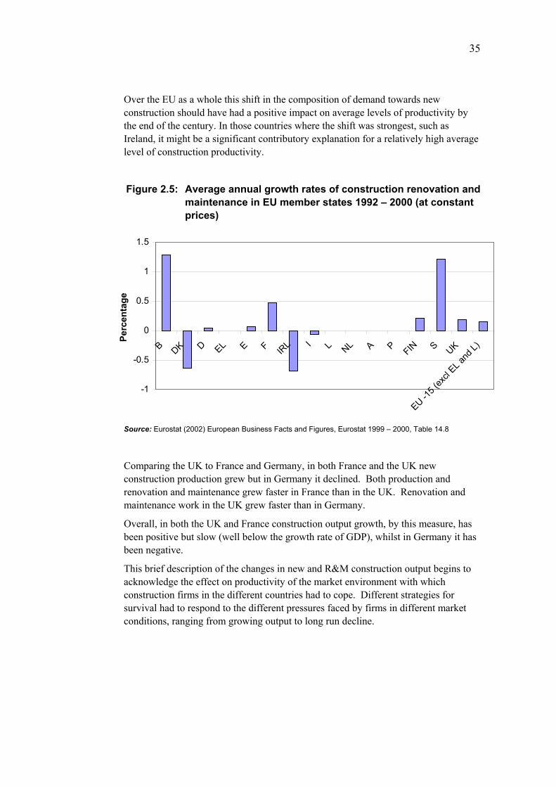
35

Over the EU as a whole this shift in the composition of demand towards new construction should have had a positive impact on average levels of productivity by the end of the century. In those countries where the shift was strongest, such as Ireland, it might be a significant contributory explanation for a relatively high average level of construction productivity.

Figure 2.5: Average annual growth rates of construction renovation and maintenance in EU member states 1992 – 2000 (at constant prices)

-1

-0.5

0

0.5

1

1.5

B DK D EL E F IRL I L NL A P FIN S UK

EU -15 (

excl

EL and

L)

Perc

enta

ge

Source: Eurostat (2002) European Business Facts and Figures, Eurostat 1999 – 2000, Table 14.8

Comparing the UK to France and Germany, in both France and the UK new construction production grew but in Germany it declined. Both production and renovation and maintenance grew faster in France than in the UK. Renovation and maintenance work in the UK grew faster than in Germany.

Overall, in both the UK and France construction output growth, by this measure, has been positive but slow (well below the growth rate of GDP), whilst in Germany it has been negative.

This brief description of the changes in new and R&M construction output begins to acknowledge the effect on productivity of the market environment with which construction firms in the different countries had to cope. Different strategies for survival had to respond to the different pressures faced by firms in different market conditions, ranging from growing output to long run decline.

36

(c) The effect of activity-composition of output on productivity levels

Building of structures, Installation, Completion

It is possible in principle to compare these three main sub-sectors of construction activity using Eurostat NewCronos data. It is just possible that the severe reservations about this data source expressed above do not invalidate its use to measure relative productivity levels in the sub-sectors of a single country

Table 2.17 shows that in France, Germany and the UK differences in reported labour productivity between 45.1, 45.2, 45.3 and 45.4 are modest. In each country, 45.1 (site preparation) has somewhat higher productivity than the average for 45.

Table 2.17: Construction value-added per employee 1999-2001 (€ 000s)

45 1999 2000 2001 45.3 1999 2000 2001 Germany 34.4 34.5 34 Germany 31.2 31.1 32.2 France 31.5 34.1 35.7 France 32.3 34.7 36.3 UK 44 49.5 55.9 UK 38.8 45.3 47.9 45.1 1999 2000 2001 45.4 1999 2000 2001 Germany 41.8 39.2 36.5 Germany 28.8 29.5 28.5 France 36.5 38.9 41.2 France 28.4 31 32.7 UK 50.5 59.8 61.6 UK 37.9 45.9 49.2 45.2 1999 2000 2001 45.5 1999 2000 2001 Germany 38.6 38.7 37.9 Germany na na 61 France 32.2 34.9 36.4 France 49.1 54.7 50.6 UK 47.1 51.9 60.7 UK 52.5 51.3 57.4

Source: Eurostat NewCronos (2003) Structural Business Statistics Database, Collection: Enterpr, Table:

Enter_MS.

If, in each of the UK, France and Germany, we set LP per employee in the whole of SIC 45 as 100, then Table 2.18 shows the highest and lowest relative levels of productivity in any of the three substantial 3-digit sub-sectors i.e. excluding 45.1 and 45.5 (see pp39-40 for the case for their exclusion).

These results are in the direction expected, given the greater technical possibilities for mechanisation in building of structures and civil engineering (45.2), and indeed in UK and Germany (though not in France) we find relatively higher levels of GFCF-P (gross capital expenditure on plant and machinery) per head in this sub-sector than in 45.3 and 45.4.

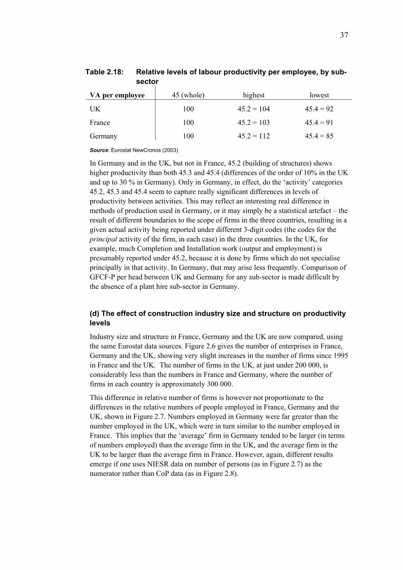
37

Table 2.18: Relative levels of labour productivity per employee, by sub-sector

VA per employee 45 (whole) highest lowest

UK 100 45.2 = 104 45.4 = 92

France 100 45.2 = 103 45.4 = 91

Germany 100 45.2 = 112 45.4 = 85

Source: Eurostat NewCronos (2003)

In Germany and in the UK, but not in France, 45.2 (building of structures) shows higher productivity than both 45.3 and 45.4 (differences of the order of 10% in the UK and up to 30 % in Germany). Only in Germany, in effect, do the ‘activity’ categories 45.2, 45.3 and 45.4 seem to capture really significant differences in levels of productivity between activities. This may reflect an interesting real difference in methods of production used in Germany, or it may simply be a statistical artefact – the result of different boundaries to the scope of firms in the three countries, resulting in a given actual activity being reported under different 3-digit codes (the codes for the principal activity of the firm, in each case) in the three countries. In the UK, for example, much Completion and Installation work (output and employment) is presumably reported under 45.2, because it is done by firms which do not specialise principally in that activity. In Germany, that may arise less frequently. Comparison of GFCF-P per head between UK and Germany for any sub-sector is made difficult by the absence of a plant hire sub-sector in Germany.

(d) The effect of construction industry size and structure on productivity levels

Industry size and structure in France, Germany and the UK are now compared, using the same Eurostat data sources. Figure 2.6 gives the number of enterprises in France, Germany and the UK, showing very slight increases in the number of firms since 1995 in France and the UK. The number of firms in the UK, at just under 200 000, is considerably less than the numbers in France and Germany, where the number of firms in each country is approximately 300 000.

This difference in relative number of firms is however not proportionate to the differences in the relative numbers of people employed in France, Germany and the UK, shown in Figure 2.7. Numbers employed in Germany were far greater than the number employed in the UK, which were in turn similar to the number employed in France. This implies that the ‘average’ firm in Germany tended to be larger (in terms of numbers employed) than the average firm in the UK, and the average firm in the UK to be larger than the average firm in France. However, again, different results emerge if one uses NIESR data on number of persons (as in Figure 2.7) as the numerator rather than CoP data (as in Figure 2.8).

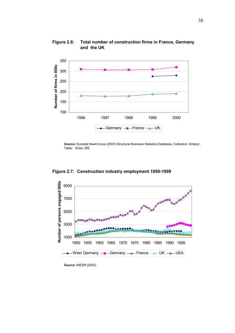
38

Figure 2.6: Total number of construction firms in France, Germany and the UK

100

150

200

250

300

350

1996 1997 1998 1999 2000

Num

ber o

f firm

s in

000

s

Germany France UK

Source: Eurostat NewCronos (2003) Structural Business Statistics Database, Collection: Enterpr, Table: Enter_MS.

Figure 2.7: Construction industry employment 1950-1999

1000

3000

5000

7000

9000

1950 1955 1960 1965 1970 1975 1980 1985 1990 1995Num

ber o

f per

sons

eng

aged

000

s

West Germany Germany France UK USA

Source: NIESR (2003)

39

Figure 2.8: Number of persons employed in construction (SIC 45) 1996-2000

500

1,000

1,500

2,000

2,500

1996 1997 1998 1999 2000

Num

ber o

f em

ploy

ees

000s

Germany France UK

Source: Eurostat NewCronos (2003) Structural Business Statistics Database, Collection: Enterpr,

Table:Enter_MS.

Figure 2.9: Number of all construction firms employing 20 or more

persons

0

5

10

15

20

25

30

1995 1996 1997 1998 1999 2000

Num

ber o

f firm

s 00

0s

Germany France UK

Source: Eurostat NewCronos (2003) Structural Business Statistics Database, Collection: Enterpr, Table:

ENT_L_MS.

Of all enterprises in each of these countries less than 10 per cent of firms employ 20 persons or more. In France the proportion is less than 3 per cent. Figure 2.9 shows the number of firms employing 20 or more persons in each respective country. The main feature shown in Figure 2.9 is the marked decline in the number of these larger

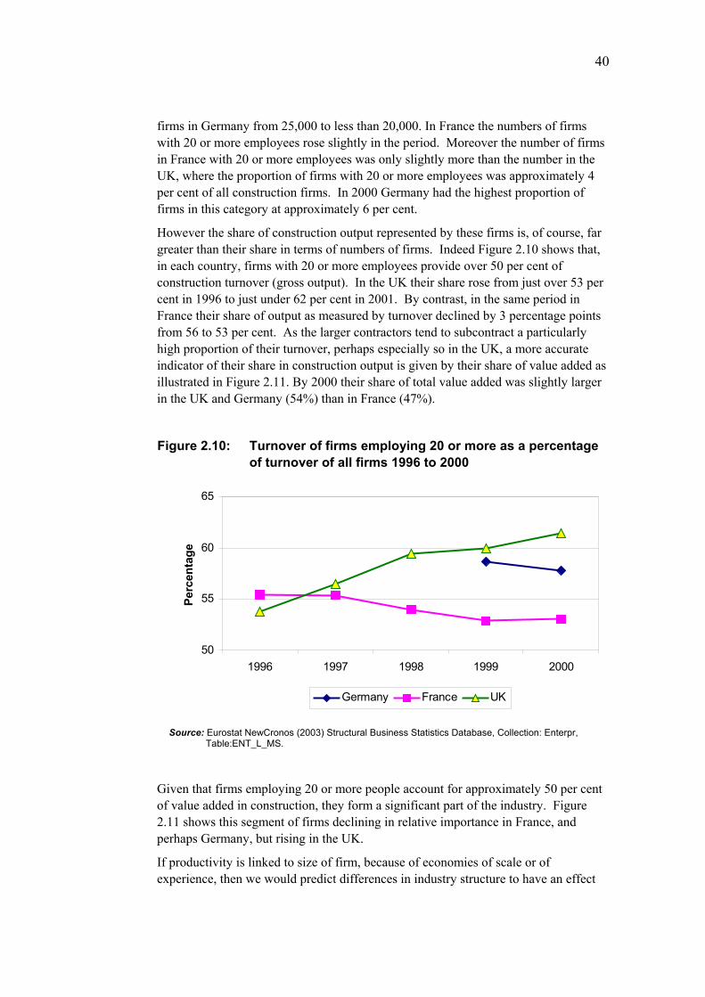
40

firms in Germany from 25,000 to less than 20,000. In France the numbers of firms with 20 or more employees rose slightly in the period. Moreover the number of firms in France with 20 or more employees was only slightly more than the number in the UK, where the proportion of firms with 20 or more employees was approximately 4 per cent of all construction firms. In 2000 Germany had the highest proportion of firms in this category at approximately 6 per cent.

However the share of construction output represented by these firms is, of course, far greater than their share in terms of numbers of firms. Indeed Figure 2.10 shows that, in each country, firms with 20 or more employees provide over 50 per cent of construction turnover (gross output). In the UK their share rose from just over 53 per cent in 1996 to just under 62 per cent in 2001. By contrast, in the same period in France their share of output as measured by turnover declined by 3 percentage points from 56 to 53 per cent. As the larger contractors tend to subcontract a particularly high proportion of their turnover, perhaps especially so in the UK, a more accurate indicator of their share in construction output is given by their share of value added as illustrated in Figure 2.11. By 2000 their share of total value added was slightly larger in the UK and Germany (54%) than in France (47%).

Figure 2.10: Turnover of firms employing 20 or more as a percentage of turnover of all firms 1996 to 2000

50

55

60

65

1996 1997 1998 1999 2000

Perc

enta

ge

Germany France UK

Source: Eurostat NewCronos (2003) Structural Business Statistics Database, Collection: Enterpr, Table:ENT_L_MS.

Given that firms employing 20 or more people account for approximately 50 per cent of value added in construction, they form a significant part of the industry. Figure 2.11 shows this segment of firms declining in relative importance in France, and perhaps Germany, but rising in the UK.

If productivity is linked to size of firm, because of economies of scale or of experience, then we would predict differences in industry structure to have an effect

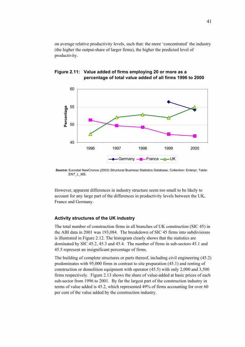
41

on average relative productivity levels, such that: the more ‘concentrated’ the industry (the higher the output-share of larger firms), the higher the predicted level of productivity.

Figure 2.11: Value added of firms employing 20 or more as a percentage of total value added of all firms 1996 to 2000

45

50

55

60

1996 1997 1998 1999 2000

Perc

enta

ge

Germany France UK

Source: Eurostat NewCronos (2003) Structural Business Statistics Database, Collection: Enterpr, Table: ENT_L_MS.

However, apparent differences in industry structure seem too small to be likely to account for any large part of the differences in productivity levels between the UK, France and Germany.

Activity structures of the UK industry

The total number of construction firms in all branches of UK construction (SIC 45) in the ABI data in 2001 was 193,084. The breakdown of SIC 45 firms into subdivisions is illustrated in Figure 2.12. The histogram clearly shows that the statistics are dominated by SIC 45.2, 45.3 and 45.4. The number of firms in sub-sectors 45.1 and 45.5 represent an insignificant percentage of firms.

The building of complete structures or parts thereof, including civil engineering (45.2) predominates with 95,000 firms in contrast to site preparation (45.1) and renting of construction or demolition equipment with operator (45.5) with only 2,000 and 3,500 firms respectively. Figure 2.13 shows the share of value-added at basic prices of each sub-sector from 1996 to 2001. By far the largest part of the construction industry in terms of value added is 45.2, which represented 49% of firms accounting for over 60 per cent of the value added by the construction industry.

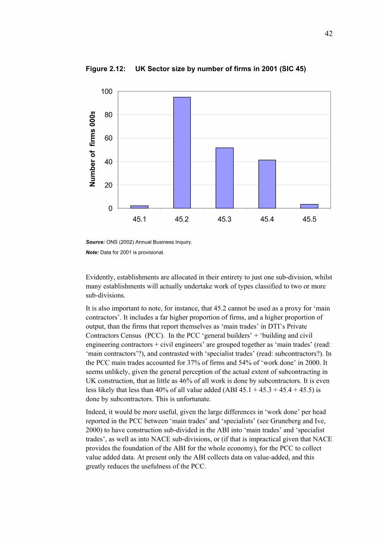
42

Figure 2.12: UK Sector size by number of firms in 2001 (SIC 45)

0

20

40

60

80

100

45.1 45.2 45.3 45.4 45.5

Num

ber o

f fir

ms

000s

Source: ONS (2002) Annual Business Inquiry.

Note: Data for 2001 is provisional.

Evidently, establishments are allocated in their entirety to just one sub-division, whilst many establishments will actually undertake work of types classified to two or more sub-divisions.

It is also important to note, for instance, that 45.2 cannot be used as a proxy for ‘main contractors’. It includes a far higher proportion of firms, and a higher proportion of output, than the firms that report themselves as ‘main trades’ in DTI’s Private Contractors Census (PCC). In the PCC ‘general builders’ + ‘building and civil engineering contractors + civil engineers’ are grouped together as ‘main trades’ (read: ‘main contractors’?), and contrasted with ‘specialist trades’ (read: subcontractors?). In the PCC main trades accounted for 37% of firms and 54% of ‘work done’ in 2000. It seems unlikely, given the general perception of the actual extent of subcontracting in UK construction, that as little as 46% of all work is done by subcontractors. It is even less likely that less than 40% of all value added (ABI 45.1 + 45.3 + 45.4 + 45.5) is done by subcontractors. This is unfortunate.

Indeed, it would be more useful, given the large differences in ‘work done’ per head reported in the PCC between ‘main trades’ and ‘specialists’ (see Gruneberg and Ive, 2000) to have construction sub-divided in the ABI into ‘main trades’ and ‘specialist trades’, as well as into NACE sub-divisions, or (if that is impractical given that NACE provides the foundation of the ABI for the whole economy), for the PCC to collect value added data. At present only the ABI collects data on value-added, and this greatly reduces the usefulness of the PCC.

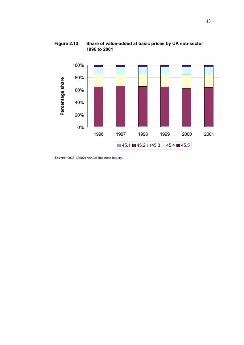
43

Figure 2.13: Share of value-added at basic prices by UK sub-sector 1996 to 2001

0%

20%

40%

60%

80%

100%

1996 1997 1998 1999 2000 2001

Perc

enta

ge s

hare

45.1 45.2 45.3 45.4 45.5

Source: ONS, (2002) Annual Business Inquiry.

44

3 International comparison of rates of change and trends of construction productivity

International comparison of productivity growth rates serves different purposes to that of comparison of levels. It is now perhaps most commonly used to benchmark performance improvement. One exceptional difficulty, for comparison of rates of change in construction productivity, arises from the very different methods adopted internationally in deflation of output value to constant prices.

Introduction: Price deflators to convert construction output to constant prices

Output, in the NIESR data set, is gross value added at constant prices. In the UK these are at constant factor cost, and are as given in the Blue Book. For the US and Germany, constant price VA is ‘double deflated’ and is calculated as gross output deflated by producer prices minus intermediate output deflated by intermediate input prices. We will see below (in the special section on US construction productivity) that this method, as applied in practice, is believed to create major distortion because of the absence of accurate indices for construction industry intermediate input and construction output prices.

During their work for Eurostat on construction PPPs, DLC have reviewed the scope and reliability of general construction output price deflators in EU and OECD countries. With very few exceptions, notably the UK and Finland, the construction deflators available are limited in both scope and coverage. Generally, input cost indices are available, but output price indices much less so. Within this generic limitation, housing and infrastructure indices tend to be more widely available, and based on better data sets, than indices for non-residential building work.

For countries that use input cost indices as output deflators, the real question that a user of the data interested in productivity trends must ask is not: ‘what do the data appear to show for changes in value of construction output at constant prices (and thus what do they show for productivity change when brought alongside a labour input series)?’; but rather: ‘what assumptions about or what methods of estimation of the rate of productivity change have already been made by those producing the output series?’ For example, it is commonplace for repair & maintenance ‘price’ deflators to be in reality cost indices based on an assumption of constant labour productivity (so that a wage index can be used as a labour cost index). In this case an assumed rate of productivity growth (zero) has already been built-in. It is pointless to try to then use the resulting series for ‘constant price’ output to estimate that very rate.

In short-run comparisons of rates of productivity change, ‘price’ deflators based on input-cost indices suffer from a further disadvantage: namely, the tendency for the ratio of construction output prices to input prices to widen (grow) during construction booms and then to shrink (fall) during recessions.

It may sometimes be preferable to use a general ‘GDP deflator’ or a deflator for prices of all capital goods, rather than specific construction ‘price’ deflators that are really input-cost indices.

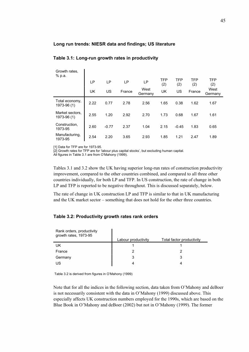
45

Long run trends: NIESR data and findings; US literature

Table 3.1: Long-run growth rates in productivity

Growth rates, % p.a.

LP LP LP LP TFP (2)

TFP (2)

TFP (2)

TFP (2)

UK US France West

Germany UK US France West Germany

Total economy, 1973-96 (1) 2.22 0.77 2.78 2.56 1.65 0.38 1.62 1.67

Market sectors, 1973-96 (1) 2.55 1.20 2.92 2.70 1.73 0.68 1.67 1.61

Construction, 1973-95 2.60 -0.77 2.37 1.04 2.15 -0.45 1.83 0.65

Manufacturing, 1973-95 2.54 2.20 3.65 2.93 1.85 1.21 2.47 1.89

[1] Data for TFP are for 1973-95. [2] Growth rates for TFP are for ‘labour plus capital stocks’, but excluding human capital.

All figures in Table 3.1 are from O’Mahony (1999).

Tables 3.1 and 3.2 show the UK having superior long-run rates of construction productivity improvement, compared to the other countries combined, and compared to all three other countries individually, for both LP and TFP. In US construction, the rate of change in both LP and TFP is reported to be negative throughout. This is discussed separately, below.

The rate of change in UK construction LP and TFP is similar to that in UK manufacturing and the UK market sector – something that does not hold for the other three countries.

Table 3.2: Productivity growth rates rank orders

Rank orders, productivity growth rates, 1973-95

Labour productivity Total factor productivity UK 1 1 France 2 2 Germany 3 3 US 4 4

Table 3.2 is derived from figures in O’Mahony (1999)

Note that for all the indices in the following section, data taken from O’Mahony and deBoer is not necessarily consistent with the data in O’Mahony (1999) discussed above. This especially affects UK construction numbers employed for the 1990s, which are based on the Blue Book in O’Mahony and deBoer (2002) but not in O’Mahony (1999). The former

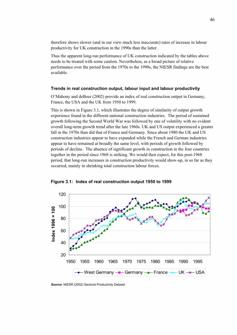
46

therefore shows slower (and in our view much less inaccurate) rates of increase in labour productivity for UK construction in the 1990s than the latter.

Thus the apparent long-run performance of UK construction indicated by the tables above needs to be treated with some caution. Nevertheless, as a broad picture of relative performance over the period from the 1970s to the 1990s, the NIESR findings are the best available.

Trends in real construction output, labour input and labour productivity

O’Mahony and deBoer (2002) provide an index of real construction output in Germany, France, the USA and the UK from 1950 to 1999.

This is shown in Figure 3.1, which illustrates the degree of similarity of output growth experience found in the different national construction industries. The period of sustained growth following the Second World War was followed by one of volatility with no evident overall long-term growth trend after the late 1960s. UK and US output experienced a greater fall in the 1970s than did that of France and Germany. Since about 1980 the UK and US construction industries appear to have expanded while the French and German industries appear to have remained at broadly the same level, with periods of growth followed by periods of decline. The absence of significant growth in construction in the four countries together in the period since 1968 is striking. We would then expect, for this post-1968 period, that long-run increases in construction productivity would show-up, in so far as they occurred, mainly in shrinking total construction labour forces.

Figure 3.1: Index of real construction output 1950 to 1999

20

40

60

80

100

120

1950 1955 1960 1965 1970 1975 1980 1985 1990 1995

Inde

x 19

96 =

100

West Germany Germany France UK USA

Source: NIESR (2002) Sectoral Productivity Dataset

47

Figure 3.2 compares the trends in number employed of the national construction industries of the four countries from 1950 to 1999, including the break caused by German re-unification. While the trends in employment appear to have followed a similar pattern in all the European countries shown, peaking in the late 1960s or early 1970s, and slowly falling thereafter, the trend in employment in the construction industry in the USA appears to show a rapidly increasing trend in the number of persons engaged in construction activities. This is discussed below, in the special section on the US.

Figure 3.2: Construction industry employment 1950 to 1999

0

2

4

6

8

10

1950

1953

1956

1959

1962

1965

1968

1971

1974

1977

1980

1983

1986

1989

1992

1995

1998

Num

ber o

f per

sons

in m

illio

ns

West Germany Germany France UK USA

Source: NIESR (2002) Sectoral Productivity Dataset

A clue that these differences might be due in part to factors outside construction is given by Figure 3.3, which shows construction employment as a percentage of total employment in the different countries studied. The growth in employment in construction in the USA is not reflected in growth in its share of total employment. In other words, employment in the US construction industry expanded at the same rate as employment in other sectors.

However, whereas in the period up to 1968, this growing level of employment in US construction is modest and arises largely because construction output in the US is growing rapidly (and the growth in employment is slower than the growth in output, signalling a rising trend in labour productivity), after that date it seems to indicate a significant and sustained decline in US construction productivity, as only thus could so many more workers be required to produce an output that grew only relatively slowly.

On the other hand, in the three European countries, total employment in the whole economy rose, after 1970, much more slowly than in the US, but this was still sufficient (given the absence of construction output, and thus employment, growth after 1970) to cause construction’s share in total employment to fall slowly. Indeed following a period of relative

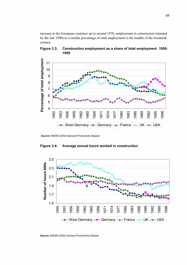
48

increase in the European countries up to around 1970, employment in construction returned by the late 1990s to a similar percentage of total employment to the middle of the twentieth century.

Figure 3.3: Construction employment as a share of total employment 1950-1999

4

5

6

7

8

9

10

11

1950

1953

1956

1959

1962

1965

1968

1971

1974

1977

1980

1983

1986

1989

1992

1995

1998

Perc

enta

ge o

f tot

al e

mpl

oym

ent

West Germany Germany France UK USA

Source: NIESR (2002) Sectoral Productivity Dataset

Figure 3.4: Average annual hours worked in construction

1.5

1.7

1.9

2.1

2.3

2.5

1950

1953

1956

1959

1962

1965

1968

1971

1974

1977

1980

1983

1986

1989

1992

1995

1998

Num

ber o

f hou

rs 0

00s

West Germany Germany France UK USA

Source: NIESR (2002) Sectoral Productivity Dataset

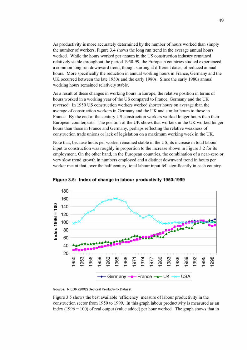
49

As productivity is more accurately determined by the number of hours worked than simply the number of workers, Figure 3.4 shows the long run trend in the average annual hours worked. While the hours worked per annum in the US construction industry remained relatively stable throughout the period 1950-99, the European countries studied experienced a common long run downward trend, though starting at different dates, of reduced annual hours. More specifically the reduction in annual working hours in France, Germany and the UK occurred between the late 1950s and the early 1980s. Since the early 1980s annual working hours remained relatively stable.

As a result of these changes in working hours in Europe, the relative position in terms of hours worked in a working year of the US compared to France, Germany and the UK reversed. In 1950 US construction workers worked shorter hours on average than the average of construction workers in Germany and the UK and similar hours to those in France. By the end of the century US construction workers worked longer hours than their European counterparts. The position of the UK shows that workers in the UK worked longer hours than those in France and Germany, perhaps reflecting the relative weakness of construction trade unions or lack of legislation on a maximum working week in the UK.

Note that, because hours per worker remained stable in the US, its increase in total labour input to construction was roughly in proportion to the increase shown in Figure 3.2 for its employment. On the other hand, in the European countries, the combination of a near-zero or very slow trend growth in numbers employed and a distinct downward trend in hours per worker meant that, over the half century, total labour input fell significantly in each country.

Figure 3.5: Index of change in labour productivity 1950-1999

20

40

60

80

100

120

140

160

180

1950

1953

1956

1959

1962

1965

1968

1971

1974

1977

1980

1983

1986

1989

1992

1995

1998

Inde

x 19

96 =

100

Germany France UK USA

Source: NIESR (2002) Sectoral Productivity Dataset

Figure 3.5 shows the best available ‘efficiency’ measure of labour productivity in the construction sector from 1950 to 1999. In this graph labour productivity is measured as an index (1996 = 100) of real output (value added) per hour worked. The graph shows that in

50

the last quarter of the 20th century both France and the UK increased their productivity per annum while productivity fell in the US. Although this implies that the productivity gap narrowed it does not, of course, imply that productivity in the European countries studied had caught up or overtaken the US by 1999.

Table 3.3 shows that from 1950 to 1999, while productivity in France and the UK improved by 3 per cent per annum and 2 per cent per annum respectively, productivity in the US construction industry, according to the data, declined by 0.76 per cent per annum. Having followed a pattern of annual productivity improvements from 1950 to 1965, the index of labour productivity declined until 1981. In this period, 1965-81, US construction output fell somewhat but the number of persons engaged in the US construction industry increased by 50 per cent in the same period. (See section on the US at the end of this chapter.)

Table 3.3: Long run average annual productivity growth rate 1950 to 1999

Country Log regression annual average rate of change R2

France 3.00 0.97 Germany 0.3 0.33 USA -0.76 0.37 UK 2.00 0.96

Note: Based on data given in the NIESR (2002) Sectoral Productivity Dataset

Unfortunately, the NIESR dataset does not contain values for construction real output (value added at constant prices), but only indices for real output. Consequently, it likewise only contains indices for labour productivity. Relative levels (but not values) of productivity are given for 1996 and 1999.

Estimation of relative levels for other years is possible by applying the respective NIESR productivity indices to these base-year relative levels. However, it is then impossible to make direct comparison of NIESR estimates for values of real output in a particular year with alternative estimates.

Thus, of the three possible constituent sources of differences in estimates between NIESR and others for levels of labour productivity at any point in time:

Differences in estimated constant-price national currency value of output (arising from use of different primary value added data or from different base years for deflators or methods of deflation);

Differences in method used for converting national currencies to a common unit in terms of purchasing power equivalence; Differences in estimated labour input;

we are able directly only to observe the third.

Interpreting the US time series for construction productivity

There is a substantial literature on this topic, most of it recently focusing upon apparent discrepancies between estimates of construction productivity trends derived from aggregate data (which show long-term and continuing declines in construction labour productivity,

51

broadly in line with the NIESR findings reported above) and estimates derived from site-based or activity-based studies (which show increases in construction labour productivity over time).

Goodrum et al (2002), Goodrum and Haas (2002) and Allmon et al (2000) provide good overviews of this literature, as well as containing significant new contributions thereto. Griliches (1988) and Eisner (1994) are important slightly older contributions that also question the apparent productivity decline.

Activity-sampling studies (Goodrum et al, 2002) show rising labour productivity for those activities that remain on-site. Partial reconciliation with aggregate data showing falling productivity, without invalidating the latter, would require that the remaining on-site activities (at the end of a long period of increasing prefabrication) have, on average, lower labour productivity than those activities formerly undertaken on-site but since transferred off-site. However, this would imply a dynamic rather than static effect of economic incentives on the drive to prefabricate. Ordinarily, in comparative static analyses, the incentive to prefabricate will be greatest for activities with below-average levels of on-site labour productivity, because here the savings in construction labour cost will be proportionately greater. But, more dynamically: some on-site activities will be technically easier to mechanise (efficiently) than others. We would expect the ‘mechanisable’ activities to remain on-site, and show above average increases in labour productivity over time reflecting this increased mechanisation (increased plant and equipment per worker); and expect the effort to switch activities off-site to focus on the less mechanisable activities. If the more ‘mechanisable’ activities began the period with lower-than-average labour productivity, this version of choice of path of technique (choice between mechanisation and prefabrication of activities) could help to some extent to reconcile the findings of the site-based and aggregate studies.

However this may be, it cannot explain all of the discrepancy. Most recent researchers have come to the conclusion that it is the aggregate data which is flawed, and which gives a misleading picture of ‘actual’ productivity trends.

The US data on construction output (and value added) at current prices is probably neither more nor less accurate in its capture of actual rates of change than that of the other countries in this study. That is, in all cases there is a significant amount of unrecorded output, for which some attempted correction is made by the national statistical institutes, using input-output data and other sources. In all cases, the net result is probably a figure that understates ‘actual’ construction industry output. This need not, however, invalidate either cross-country or time series analyses, so long as the relative proportion of unrecorded output (a) is similar between countries (for cross-country comparisons) and/or (b) remains stable over time in each country (for time series analyses). The latter is more plausible than the former, perhaps.

The main problem with the US data on construction output comes when it is attempted to deflate output at current prices into a time series of output at constant prices. The method used in the US is this. Starting with series for gross output of construction and for intermediate inputs into construction, a series for construction value added is derived by a method called ‘double deflation’. In this method, gross output is deflated by a price index which attempts to measure purchasers’ prices paid (‘market prices’, including indirect taxes

52

and any margin charged by intermediaries such as developers, on top of producers’ prices received), whilst intermediate input is deflated by a materials cost index (which attempts to measure prices paid by construction firms to purchase inputs, but which in some cases measures prices received by materials producers).

Unfortunately, the gross output deflator used is in fact largely a housing price index, the Census Bureau Single-Family Houses Under Construction Index (more than half of all US construction output is deflated using this index). The assumptions behind use of this index are:

(a) that the great majority of new houses are built by contractors working to order to a non-construction-industry client, so that a construction contract is placed whose value includes only payments to a construction firm for construction work, with no element of land price; or

(b) that the firm making the return is able accurately to deduct land value (called ‘lot price’); or

(c) that the NSI has an alternative accurate source for lot prices, enabling it to make the deduction; and

(d) that an index of new housing construction price can be applied as representative of prices for all types of construction work.

None of these assumptions appears likely to be valid. In the case of assumptions (a) to (c), problems will arise if owner-occupiers either purchase new houses together with the land on which they stand (from builder-developers), or purchase the construction output from a real estate development company that is not classified as belonging to the construction industry (and which has itself engaged a contractor or contractors).

In the case of assumption (d), the problems are perhaps too obvious to require further elaboration. There is anyway clear evidence that this index is affected by conditions in the US housing market, that have only marginal relevance for the construction contract prices of non-housing new projects, or for the contract prices of repair & maintenance work of any kind.

The US government statistical service is forced to resort to this expedient because of the absence in the US of an equivalent to the UK system of Bills of Quantities. It is this system that, in the UK, permits construction tender and output price indices to be produced. Heterogeneous projects all comprise various measured quantities of the same set of constituent elements, each of which is priced by the contractor. The price index tracks changes in the prices of a representative ‘basket’ of these elements.

Thus, the US Bureau of Labor Statistics, for example, produces time series and indices for productivity in every other major industry in the US economy, but declines to do so for construction, because of its awareness of the extreme inadequacies of the only available price deflator for construction output.

Broadly, it seems likely that prices paid by purchasers of new houses (after deducting ‘estimated’ lot price) have been rising faster than actual all-construction output prices, in part because of (unadjusted) improvements in housing quality, and in part because long financial

53

and housing market booms have stimulated all house prices, including prices paid for new houses.

It is also possible, insofar as the Single-Family Houses Under Construction Index reflects costs of production at all, that it is unrepresentative because labour productivity in housebuilding has not increased as rapidly as in other new construction, thus causing housebuilding costs to rise faster than costs of other construction.

‘More than half of the Census Value of Construction Put in Place is converted to real output using the Single-Family Houses Under Construction Index’ (Goodrum et all, 2002, p. 416). The remainder is deflated using contractors’ input cost indices.

Real construction VA appears to have been broadly constant (more exactly: to fluctuate around a constant mean level) in the US since the late 1960s (O’Mahony, 1999, Table A). A widespread view adopted in the academic literature is that construction VA has actually been growing over this long period. The argument is as follows. Real VA appears constant only because:

(a) the house price index used to deflate over half of gross output shows increases over time well in excess of the true increases in prices for quality-improvement-adjusted units of all construction gross output;

(b) construction cost indices, including labour costs as well as intermediate input costs, produced by some agencies and private firms (Turner; Handy-Whitman; Bureau of Reclamation), and used to deflate the remainder of construction gross output, also show increases over time in excess of the ‘true’ increases in construction output prices.

Deflating output using input cost indices for units of labour and materials implies: (a) that contractors’ gross mark-ups are constant, and (b) that physical output productivity per ‘bundle’ of physical inputs is itself constant (Pieper, 1989).

The only price index, the Single-Family House index, is calculated from data on speculative housing sales prices, less estimated or reported lot (land) value, regressed on ten house characteristics including floor area, lot size, number of bathrooms, presence of garage, fireplace and air conditioning, and location (Goodrum et al, 2002).

The estimates of construction output price inflation produced by these methods are high, and do not accord with experienced industry participants’ views of actual rates of output price inflation. Moreover, deflating in this way makes no allowance for improvements in output quality over time (greater proportions of new output incorporating HVAC systems, fire protection, earthquake protection, ‘intelligent’ systems, etc.).

However, though there is overwhelming evidence that the methods of deflation currently in use will tend to understate the true level of output, and considerable evidence (based on the lack of any quality adjustment and assumption of constant ratios of output to input, including labour input) that the understatement problem will be cumulative and become more severe over time, we also need to be able to explain why the deflated output series only seems to suffer from these problems from around 1970 onwards.

Here, the ultimate explanation seems to lie in fundamental changes in construction labour market institutions and conditions that occurred at just that time.

54

From 1950 to 1968, construction real wages rose continually and by 1968 were (at between $16 and $18 1990 dollars per hour) at least 50% higher than wages in manufacturing (Goodrum et al, 2002). From 1968 to 1998, the total manufacturing real wage rate was almost constant, at around $11 1990 dollars. Over the same period, the construction real wage rate fell continuously, through most rapidly from 1972 to 1980, to around $12 1990 dollars, a fall of up to one third.

In brief, the argument is that up until 1968, exceptionally strong trade unions had successfully restricted entry to the construction labour force (not only by controlling numbers of apprenticeships and by ‘closed shops’, but also by excluding non-white workers from the industry altogether) (Linder, 1999). Thereafter, the employers launched a successful ‘open shop’ movement, defeated a series of union strikes and other forms of opposition, and opened the industry to non-union labour and to Afro-American, Hispanic and recent-migrant workers. This enabled them to recruit the required number of workers, and to increase their total workforce very considerably, whilst paying wages that were much lower both absolutely and relative to wages in manufacturing. Trade union ‘density’ in construction fell from around 70% to less than 20% over this period.

This sudden easing of labour shortages and lowering of wage rates enabled firms to be less ‘economical’ in their use of construction labour. Thus, total capital input to US construction ceased to rise after reaching a peak in 1979, and fell in total by 20% between 1979 and 1995, a period over which the labour force employed rose by 16% and ‘apparent’ real output rose by 12% (O’Mahony, 1999; Tables E, B and A).

The number of workers employed in US construction had risen only modestly during the long post-war construction boom (from 3.5 million in 1950 to 4.3 million in 1968), but then rocketed upwards to 6.0 million in 1979 and then to 7.2 million by 1996. The new and non-union workers seem to have been less productive (though cheaper to employ) than the former unionised workers.

The change over any period in apparent construction real output is a very poor predictor of the change in construction employment, in the US, over the same period. But the change in construction real wage rates is a good predictor of the change in construction capital-intensity and (inversely) in employment. The economic model at work seems to be neo-classical rather than Keynesian. In turn, the changes in construction employment (upward) and capital-intensity (downward) predict the direction of change in labour productivity (downward) – all this dependent upon a sudden relatively abundant labour supply at the wage rate offered in other sectors of the economy.

Allmon (2000) and Oppedahl (2000) agree that the fall in construction real wage rates has been caused by a rapid decrease in unionisation and in trade union power over the labour supply, by a deskilling of the workforce, and by greatly increased numbers of migrant workers in the industry.

Thus, the US shows very different trends for labour productivity when labour input is measured in physical units (numbers engaged or labour hours) than when labour input is measured in value terms, as unit labour cost.

O’Mahony (1999) points out that, as unit labour costs (the labour cost of producing one unit of output) can be defined as employment income per unit of labour input divided by

55

productivity (output per unit of labour input), and since both numerator and denominator contain labour input, this can be simplified to employment income divided by output, for the economy or for a sector. This ratio is better known as the labour share (employment income) in value added (output).

For US construction, unit labour costs (as represented by the labour share in value added) declined from the early 1950s to the late 1960s, because though wage rates rose, labour productivity rose even faster. From the late 1960s onward, these unit labour costs appear to behave cyclically, rising from 1967 to 1974, then falling to 1977, then rising to 1981, then falling to 1986, then rising to 1993. This suggests that ULC rises at the end of booms and falls in recessions and their aftermaths.

Allmon et al (2000) also use unit labour cost. They find generally declining trends for ULC, but use gross output or physical units rather than value added to measure units of output.

One recent author who has argued that construction labour productivity has declined continually, though slowly (-0.48% p.a.) over the last 30 years is Teicholz (2000; 2001). This author uses the aggregate gross output series of the Census Bureau, and its deflators (see above), and Bureau of Labor Statistics series for person-hours of labour input. This involves, inter alia, assuming that R&M output has changed over time exactly in line with new output (the Census Bureau series is for total value of new and refurbishment construction contracts).

Recently Goodrum and Haas (2001) have argued that the fall in construction real wages has contributed to keeping down the series for nominal value of construction gross output, by allowing contractors to pass on lower wage bills in lower contract prices, and thus current price values; whilst these falls in wage rates are missed by the housing price index used to deflate most of output.

Summary on the US data

Overall, we believe the best interpretation of the US data is as follows. In the late 1960s and the 1970s and into the early 1980s, there was almost certainly an actual fall in average labour productivity, as non-unionised, less skilled and much lower-paid labour replaced unionised, more skilled and higher-paid labour.

Thus at least a significant part of the fall shown by the time series for labour productivity for that period is ‘actual’.

However, since then, we believe that the problems in the deflators have tended chronically to understate the actual rate of construction real output growth, and thus to understate the rate of construction labour productivity growth, to the extent of changing its estimated sign (from positive to negative growth).

Apparent recent short run rates of change: ABI, Eurostat, NIESR

In this section we review two of the main published sources for recent international year-on-year changes in productivity: the NIESR dataset for both LP and TFP; and Eurostat NewCronos for LP, and the main national source for the UK, the ABI.

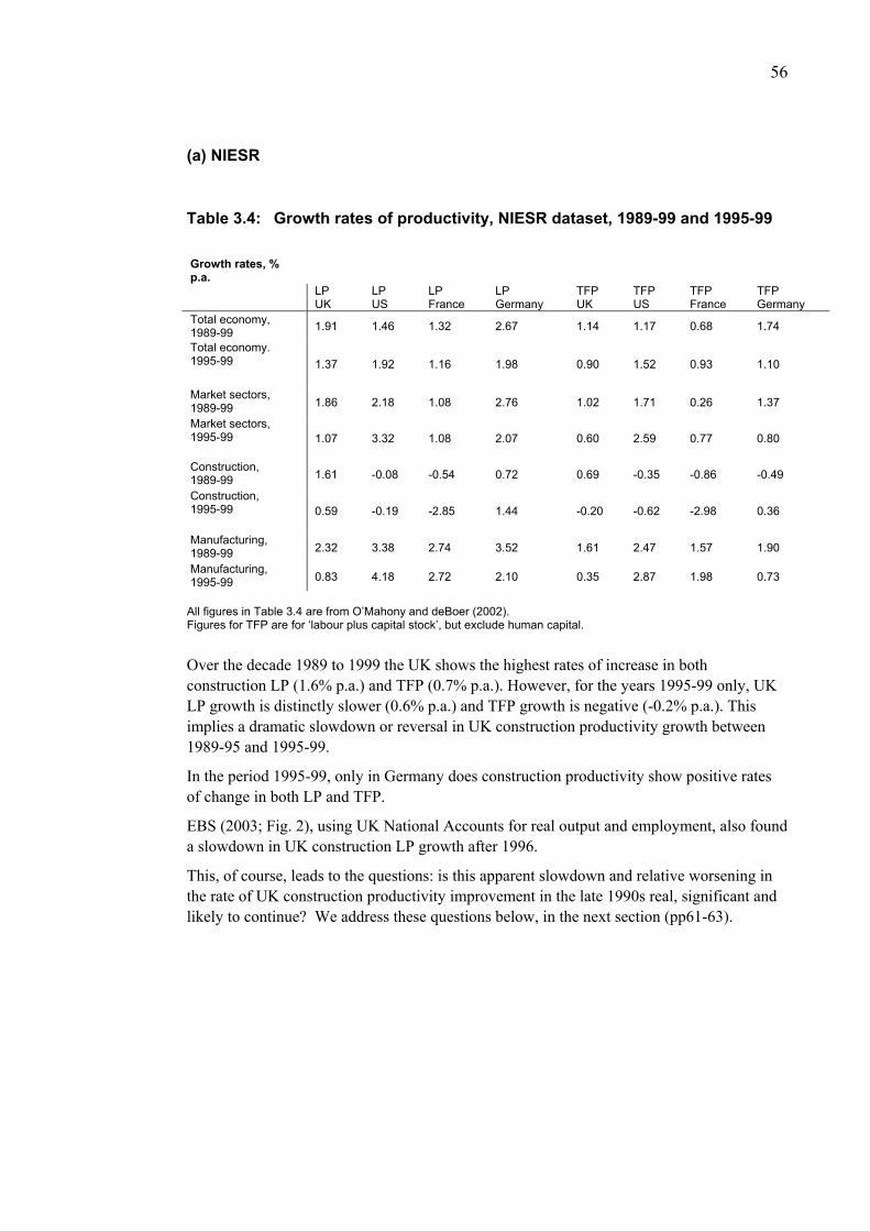
56

(a) NIESR

Table 3.4: Growth rates of productivity, NIESR dataset, 1989-99 and 1995-99

Growth rates, % p.a.

LP LP LP LP TFP TFP TFP TFP UK US France Germany UK US France Germany Total economy, 1989-99 1.91 1.46 1.32 2.67 1.14 1.17 0.68 1.74

Total economy. 1995-99 1.37 1.92 1.16 1.98 0.90 1.52 0.93 1.10

Market sectors, 1989-99 1.86 2.18 1.08 2.76 1.02 1.71 0.26 1.37

Market sectors, 1995-99 1.07 3.32 1.08 2.07 0.60 2.59 0.77 0.80

Construction, 1989-99 1.61 -0.08 -0.54 0.72 0.69 -0.35 -0.86 -0.49

Construction, 1995-99 0.59 -0.19 -2.85 1.44 -0.20 -0.62 -2.98 0.36

Manufacturing, 1989-99 2.32 3.38 2.74 3.52 1.61 2.47 1.57 1.90

Manufacturing, 1995-99 0.83 4.18 2.72 2.10 0.35 2.87 1.98 0.73

All figures in Table 3.4 are from O’Mahony and deBoer (2002). Figures for TFP are for ‘labour plus capital stock’, but exclude human capital.

Over the decade 1989 to 1999 the UK shows the highest rates of increase in both construction LP (1.6% p.a.) and TFP (0.7% p.a.). However, for the years 1995-99 only, UK LP growth is distinctly slower (0.6% p.a.) and TFP growth is negative (-0.2% p.a.). This implies a dramatic slowdown or reversal in UK construction productivity growth between 1989-95 and 1995-99.

In the period 1995-99, only in Germany does construction productivity show positive rates of change in both LP and TFP.

EBS (2003; Fig. 2), using UK National Accounts for real output and employment, also found a slowdown in UK construction LP growth after 1996.

This, of course, leads to the questions: is this apparent slowdown and relative worsening in the rate of UK construction productivity improvement in the late 1990s real, significant and likely to continue? We address these questions below, in the next section (pp61-63).

57

Table 3.5: Productivity growth rank orders Rank orders, construction productivity growth rates

LP. 1989-99 LP. 1995-99 TFP, 1989-99 TFP. 1995-99

UK 1 2 1 2 Germany 2 1 3 1 US 3 3 2 3 France 4 4 4 4

Source: O’Mahony and de Boer (2002)

ABI: apparent UK short-run changes

This section examines a number of aspects of productivity in the UK construction industry based on the Annual Business Inquiry (ABI). The ABI (2002) provides data coverage for the period 1996-2001 for most variables, however some (in particular total employment) are only available from 1998 onwards and our analysis is constrained accordingly. It gives the most recent available data, up to 2001 instead of to 1999. It also, in principle, permits disaggregation of SIC 45 into its sub-sectors.

Figure 3.6: Value added (in constant £ sterling) per employee in the UK construction industry 1985-2001

0

5

10

15

20

25

30

1985

1986

1987

1988

1989

1990

1991

1992

1993

1994

1995

1996

1997

1998

1999

2000

2001

cost

ant £

000

s

CoP ABI

Source: ONS (1988, 1992, 1998) CoP; ONS (2002) ABI

Figure 3.6 shows value added per employee in the UK construction industry over the period 1985-2001. The time series contains data from both the old Census of Production (CoP) and the new ABI. The figure clearly highlights the differences between the CoP and the ABI.

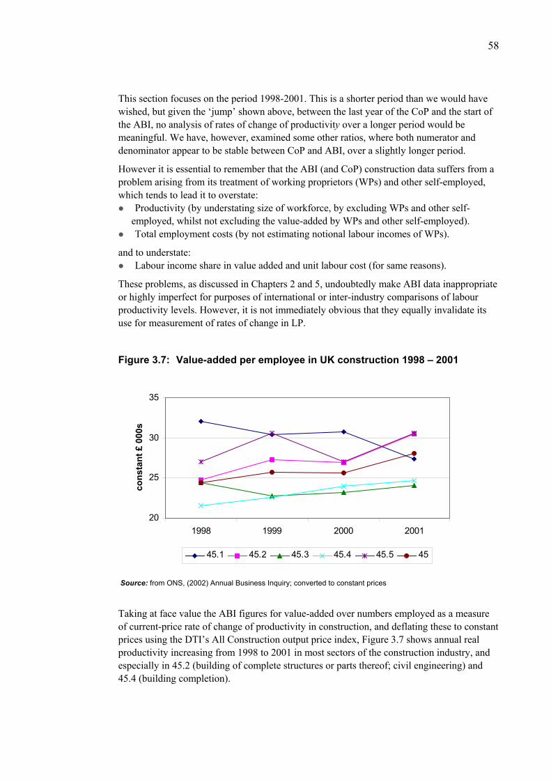
58

This section focuses on the period 1998-2001. This is a shorter period than we would have wished, but given the ‘jump’ shown above, between the last year of the CoP and the start of the ABI, no analysis of rates of change of productivity over a longer period would be meaningful. We have, however, examined some other ratios, where both numerator and denominator appear to be stable between CoP and ABI, over a slightly longer period.

However it is essential to remember that the ABI (and CoP) construction data suffers from a problem arising from its treatment of working proprietors (WPs) and other self-employed, which tends to lead it to overstate:

Productivity (by understating size of workforce, by excluding WPs and other self-employed, whilst not excluding the value-added by WPs and other self-employed).

Total employment costs (by not estimating notional labour incomes of WPs).

and to understate: Labour income share in value added and unit labour cost (for same reasons).

These problems, as discussed in Chapters 2 and 5, undoubtedly make ABI data inappropriate or highly imperfect for purposes of international or inter-industry comparisons of labour productivity levels. However, it is not immediately obvious that they equally invalidate its use for measurement of rates of change in LP.

Figure 3.7: Value-added per employee in UK construction 1998 – 2001

20

25

30

35

1998 1999 2000 2001

cons

tant

£ 0

00s

45.1 45.2 45.3 45.4 45.5 45

Source: from ONS, (2002) Annual Business Inquiry; converted to constant prices

Taking at face value the ABI figures for value-added over numbers employed as a measure of current-price rate of change of productivity in construction, and deflating these to constant prices using the DTI’s All Construction output price index, Figure 3.7 shows annual real productivity increasing from 1998 to 2001 in most sectors of the construction industry, and especially in 45.2 (building of complete structures or parts thereof; civil engineering) and 45.4 (building completion).

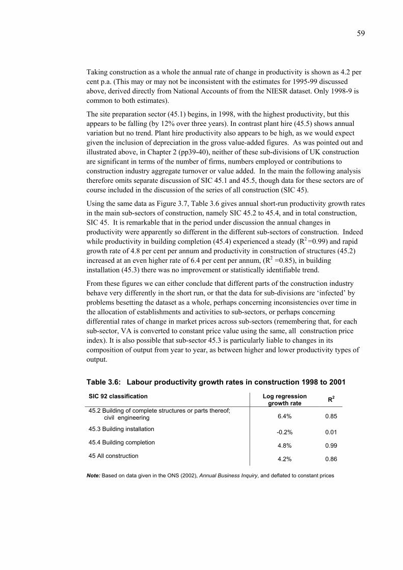
59

Taking construction as a whole the annual rate of change in productivity is shown as 4.2 per cent p.a. (This may or may not be inconsistent with the estimates for 1995-99 discussed above, derived directly from National Accounts of from the NIESR dataset. Only 1998-9 is common to both estimates).

The site preparation sector (45.1) begins, in 1998, with the highest productivity, but this appears to be falling (by 12% over three years). In contrast plant hire (45.5) shows annual variation but no trend. Plant hire productivity also appears to be high, as we would expect given the inclusion of depreciation in the gross value-added figures. As was pointed out and illustrated above, in Chapter 2 (pp39-40), neither of these sub-divisions of UK construction are significant in terms of the number of firms, numbers employed or contributions to construction industry aggregate turnover or value added. In the main the following analysis therefore omits separate discussion of SIC 45.1 and 45.5, though data for these sectors are of course included in the discussion of the series of all construction (SIC 45).

Using the same data as Figure 3.7, Table 3.6 gives annual short-run productivity growth rates in the main sub-sectors of construction, namely SIC 45.2 to 45.4, and in total construction, SIC 45. It is remarkable that in the period under discussion the annual changes in productivity were apparently so different in the different sub-sectors of construction. Indeed while productivity in building completion (45.4) experienced a steady (R2 =0.99) and rapid growth rate of 4.8 per cent per annum and productivity in construction of structures (45.2) increased at an even higher rate of 6.4 per cent per annum, (R2 =0.85), in building installation (45.3) there was no improvement or statistically identifiable trend.

From these figures we can either conclude that different parts of the construction industry behave very differently in the short run, or that the data for sub-divisions are ‘infected’ by problems besetting the dataset as a whole, perhaps concerning inconsistencies over time in the allocation of establishments and activities to sub-sectors, or perhaps concerning differential rates of change in market prices across sub-sectors (remembering that, for each sub-sector, VA is converted to constant price value using the same, all construction price index). It is also possible that sub-sector 45.3 is particularly liable to changes in its composition of output from year to year, as between higher and lower productivity types of output.

Table 3.6: Labour productivity growth rates in construction 1998 to 2001

SIC 92 classification Log regression growth rate R2

45.2 Building of complete structures or parts thereof; civil engineering 6.4% 0.85

45.3 Building installation -0.2% 0.01

45.4 Building completion 4.8% 0.99

45 All construction 4.2% 0.86

Note: Based on data given in the ONS (2002), Annual Business Inquiry, and deflated to constant prices

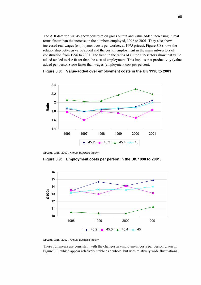
60

The ABI data for SIC 45 show construction gross output and value added increasing in real terms faster than the increase in the numbers employed, 1998 to 2001. They also show increased real wages (employment costs per worker, at 1995 prices). Figure 3.8 shows the relationship between value added and the cost of employment in the main sub-sectors of construction from 1996 to 2001. The trend in the ratios of all the sub-sectors show that value added tended to rise faster than the cost of employment. This implies that productivity (value added per person) rose faster than wages (employment cost per person).

Figure 3.8: Value-added over employment costs in the UK 1996 to 2001

1.4

1.6

1.8

2

2.2

2.4

1996 1997 1998 1999 2000 2001

Rat

io

45.2 45.3 45.4 45

Source: ONS (2002), Annual Business Inquiry.

Figure 3.9: Employment costs per person in the UK 1998 to 2001.

10

11

12

13

14

15

16

1998 1999 2000 2001

£ 00

0s

45.2 45.3 45.4 45

Source: ONS (2002), Annual Business Inquiry.

These comments are consistent with the changes in employment costs per person given in Figure 3.9, which appear relatively stable as a whole, but with relatively wide fluctuations

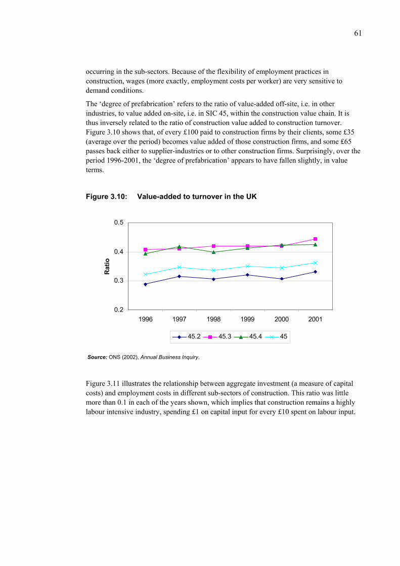
61

occurring in the sub-sectors. Because of the flexibility of employment practices in construction, wages (more exactly, employment costs per worker) are very sensitive to demand conditions.

The ‘degree of prefabrication’ refers to the ratio of value-added off-site, i.e. in other industries, to value added on-site, i.e. in SIC 45, within the construction value chain. It is thus inversely related to the ratio of construction value added to construction turnover. Figure 3.10 shows that, of every £100 paid to construction firms by their clients, some £35 (average over the period) becomes value added of those construction firms, and some £65 passes back either to supplier-industries or to other construction firms. Surprisingly, over the period 1996-2001, the ‘degree of prefabrication’ appears to have fallen slightly, in value terms.

Figure 3.10: Value-added to turnover in the UK

0.2

0.3

0.4

0.5

1996 1997 1998 1999 2000 2001

Rat

io

45.2 45.3 45.4 45

Source: ONS (2002), Annual Business Inquiry.

Figure 3.11 illustrates the relationship between aggregate investment (a measure of capital costs) and employment costs in different sub-sectors of construction. This ratio was little more than 0.1 in each of the years shown, which implies that construction remains a highly labour intensive industry, spending £1 on capital input for every £10 spent on labour input.

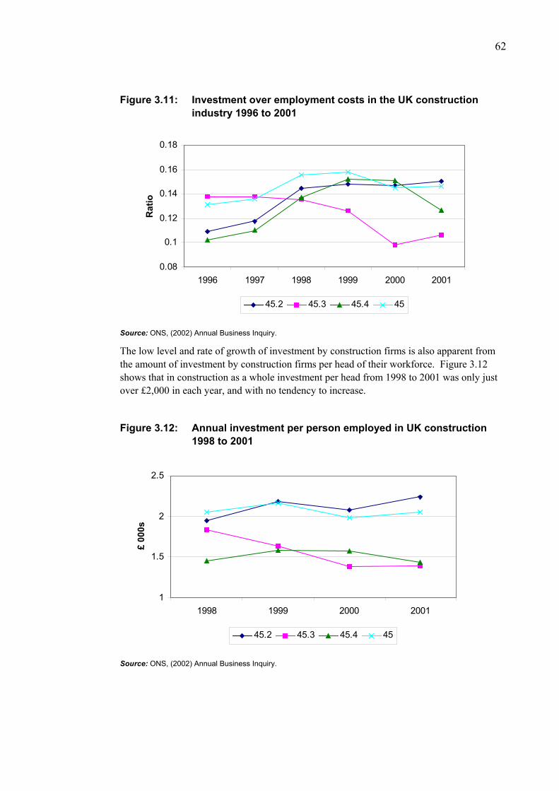
62

Figure 3.11: Investment over employment costs in the UK construction industry 1996 to 2001

0.08

0.1

0.12

0.14

0.16

0.18

1996 1997 1998 1999 2000 2001

Rat

io

45.2 45.3 45.4 45

Source: ONS, (2002) Annual Business Inquiry.

The low level and rate of growth of investment by construction firms is also apparent from the amount of investment by construction firms per head of their workforce. Figure 3.12 shows that in construction as a whole investment per head from 1998 to 2001 was only just over £2,000 in each year, and with no tendency to increase.

Figure 3.12: Annual investment per person employed in UK construction 1998 to 2001

1

1.5

2

2.5

1998 1999 2000 2001

£ 00

0s

45.2 45.3 45.4 45

Source: ONS, (2002) Annual Business Inquiry.

63

Thus it seems that neither a rising degree of prefabrication (of ex-site activities with below-average-productivity) nor rising mechanisation can explain the most recent (1998-2001) apparent increase in construction labour productivity in the UK.

(c) Eurostat NewCronos

The problems affecting the NewCronos data series for UK construction for 1995 onward were discussed at length in Chapter 2. These same problems invalidate its use for international comparisons of rates of change of labour productivity, if these comparisons are to include the UK. Thus no interpretation based on this flawed data is offered here, beyond the following comments:

Eurostat data is derived from ABI and its foreign equivalents.

We have produced estimates of short-period rates of change in LP in different sectors (45.1 to 45.5) of the three European countries’ construction industries including time series of LP for the various sub-sectors of construction. However we have been unable to find this kind of data for the USA. The source used for this was the Eurostat NewCronos database (data are in €s at current prices). Data availability has restricted the analysis to 3 years, namely 1999-2001, thus meaningful trends will be difficult to identify, although the data provides a starting point. It is essential to note that this data must not be used for comparison of levels (say, of LP levels in 45.1 in UK and in France or Germany). For the reasons discussed above, in Chapter 2, the Eurostat data seriously overstates UK construction labour productivity compared to that of Germany and, above all, France. What is true for the aggregate (SIC 45) is of course true for its components, which simply sum to the reported aggregate.

Because the reported rates of change in LP (taken from Eurostat) exclude a large, and potentially variable (see Table 3.7, below), proportion of the actual labour force in Germany and the UK (though are much more nearly ‘complete’ in coverage for France) then, even if their value added numerators are accurate, it follows that the unreliable denominators mean that we must be extremely cautious in using this source even to measure rates of change in LP.

Table 3.7: Alternative estimates of labour force: European Labour Force Surveys and Eurostat from Employer Surveys

Number employed, in 2000

ELFS (household

survey); 000s

Eurostat NewCronos;

000s

Difference, as % of ELFS

France 1501 1437 -4% Germany 3075 2263 -26% UK 1917 1339 -28%

Source: ILO (2003); Eurostat NewCronos (2003)

Recent (i.e. 1999 onwards) Eurostat data for the UK, replicate some of the problems we reported (in Chapter 2) for slightly earlier years. They appear to show ABI value added converted to euros using exchange rates, i.e. neither construction-based nor GDP-based PPPs have been used. Thus though we have tried to use Eurostat data for all three countries to maintain a consistent approach, we have very little confidence in the integrity of the data. Specifically, for the industry as a whole, i.e. SIC 45, Eurostat shows the UK’s current-price

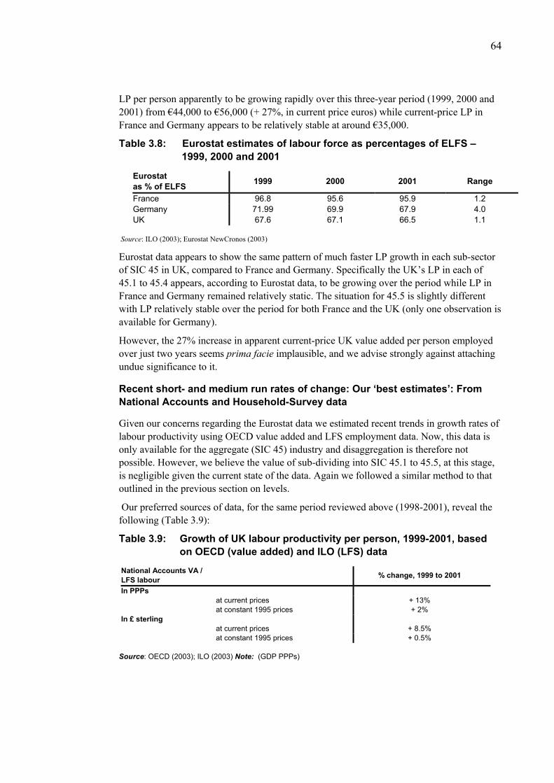
64

LP per person apparently to be growing rapidly over this three-year period (1999, 2000 and 2001) from €44,000 to €56,000 (+ 27%, in current price euros) while current-price LP in France and Germany appears to be relatively stable at around €35,000.

Table 3.8: Eurostat estimates of labour force as percentages of ELFS – 1999, 2000 and 2001

Eurostat as % of ELFS 1999 2000 2001 Range

France 96.8 95.6 95.9 1.2 Germany 71.99 69.9 67.9 4.0 UK 67.6 67.1 66.5 1.1

Source: ILO (2003); Eurostat NewCronos (2003)

Eurostat data appears to show the same pattern of much faster LP growth in each sub-sector of SIC 45 in UK, compared to France and Germany. Specifically the UK’s LP in each of 45.1 to 45.4 appears, according to Eurostat data, to be growing over the period while LP in France and Germany remained relatively static. The situation for 45.5 is slightly different with LP relatively stable over the period for both France and the UK (only one observation is available for Germany).

However, the 27% increase in apparent current-price UK value added per person employed over just two years seems prima facie implausible, and we advise strongly against attaching undue significance to it.

Recent short- and medium run rates of change: Our ‘best estimates’: From National Accounts and Household-Survey data

Given our concerns regarding the Eurostat data we estimated recent trends in growth rates of labour productivity using OECD value added and LFS employment data. Now, this data is only available for the aggregate (SIC 45) industry and disaggregation is therefore not possible. However, we believe the value of sub-dividing into SIC 45.1 to 45.5, at this stage, is negligible given the current state of the data. Again we followed a similar method to that outlined in the previous section on levels.

Our preferred sources of data, for the same period reviewed above (1998-2001), reveal the following (Table 3.9):

Table 3.9: Growth of UK labour productivity per person, 1999-2001, based on OECD (value added) and ILO (LFS) data

National Accounts VA / LFS labour

% change, 1999 to 2001

In PPPs at current prices + 13% at constant 1995 prices + 2% In £ sterling at current prices + 8.5% at constant 1995 prices + 0.5%

Source: OECD (2003); ILO (2003) Note: (GDP PPPs)

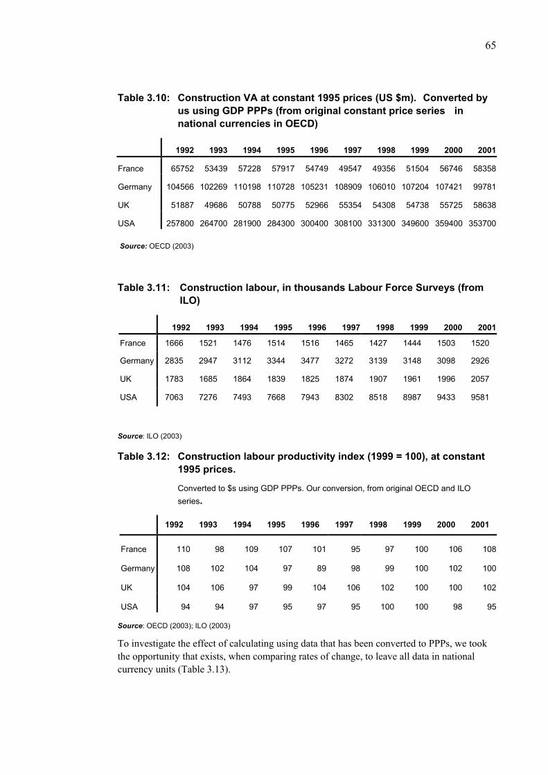
65

Table 3.10: Construction VA at constant 1995 prices (US $m). Converted by us using GDP PPPs (from original constant price series in national currencies in OECD)

1992 1993 1994 1995 1996 1997 1998 1999 2000 2001

France 65752 53439 57228 57917 54749 49547 49356 51504 56746 58358

Germany 104566 102269 110198 110728 105231 108909 106010 107204 107421 99781

UK 51887 49686 50788 50775 52966 55354 54308 54738 55725 58638

USA 257800 264700 281900 284300 300400 308100 331300 349600 359400 353700

Source: OECD (2003)

Table 3.11: Construction labour, in thousands Labour Force Surveys (from ILO)

1992 1993 1994 1995 1996 1997 1998 1999 2000 2001

France 1666 1521 1476 1514 1516 1465 1427 1444 1503 1520

Germany 2835 2947 3112 3344 3477 3272 3139 3148 3098 2926

UK 1783 1685 1864 1839 1825 1874 1907 1961 1996 2057

USA 7063 7276 7493 7668 7943 8302 8518 8987 9433 9581

Source: ILO (2003)

Table 3.12: Construction labour productivity index (1999 = 100), at constant 1995 prices.

Converted to $s using GDP PPPs. Our conversion, from original OECD and ILO series.

1992 1993 1994 1995 1996 1997 1998 1999 2000 2001

France 110 98 109 107 101 95 97 100 106 108

Germany 108 102 104 97 89 98 99 100 102 100

UK 104 106 97 99 104 106 102 100 100 102

USA 94 94 97 95 97 95 100 100 98 95

Source: OECD (2003); ILO (2003)

To investigate the effect of calculating using data that has been converted to PPPs, we took the opportunity that exists, when comparing rates of change, to leave all data in national currency units (Table 3.13).

66

Table 3.13: Construction labour productivity index (1999 = 100), at constant 1995 prices.

In national currency units. From OECD and ILO.

1992 1993 1994 1995 1996 1997 1998 1999 2000 2001

France 112 110 113 110 104 97 99 100 103 102

Germany 117 112 112 102 94 99 100 100 99 98

UK 99 104 98 99 103 103 102 100 100 101

USA 94 94 97 95 97 95 100 100 98 95

Source: OECD (2003); ILO (2003)

Our results suggest that none of the four national industries shows a significant positive trend rate of growth in labour productivity. However, all show substantial year-on-year fluctuation, perhaps related to the demand cycle.

Annual average growth rates in (GDP PPP) construction labour productivity (per person-year), 1992-2001, are:

France -0.11%

Germany -0.16%

UK -0.06%

USA +0.16%

Reasons for recent rates of change and relative productivity performance

The recent negative rate of change in labour productivity in Germany and in France may in part be attributable to the demand context in those countries in the last decade. When French and German construction output (final demand) grew over time, those industries developed ways of raising labour productivity so as to produce that growing output with a more or less constant labour force. These ways seem to have involved relatively secure long-term employment conditions, to encourage investment in human capital, and rising levels of investment per worker.

However, when faced with declining or highly volatile construction demand, these solutions may have turned into problems, giving firms higher fixed costs, and making it hard for them to cut total costs or labour input in proportion to total revenues or output in periods when revenues and output fall. Falling profits may then in turn have led to lower investment in human and fixed capital per worker, thus turning the fall in labour productivity into a long-term phenomenon.

In contrast, the UK construction industry relies on high labour flexibility, achieved by temporary- and self-employment. This is beneficial for the profit-share in value added and for labour productivity during demand downturns, but probably bad for the profit-share and bad for labour productivity towards the end of periods of demand growth, because it tends to limit labour-productivity-raising investment in human or fixed capital. Thus, especially if its construction workforce shrinks over time, the UK may be facing increasingly tight ‘capacity’

67

constraints on labour productivity (declining marginal productivity as total employment rises) whenever demand rises over a sustained period, or rises particularly rapidly. If this interpretation is correct, one would expect to see UK labour productivity growth begin to slow down if the rate of output growth experienced since 2000 continues into 2004 and beyond.

The US construction industry is different again. There, demand is still tending to increase over time. The requisite increase in output is achieved by an equally strong long-run increase in the size of the construction labour force, probably with some real increase in labour productivity as a secondary source of increased capacity. In the US as in the UK the construction labour market appears to be flexible, but with greater labour reserves to draw upon when required, to prevent labour shortages during demand upswings.

68

4 International comparison of levels of capital input per worker or per unit of output

Having described output, labour input and labour productivity we now turn to one of the main “causes” of labour productivity improvements, namely capital inputs.

Long-run changes

O’Mahony and deBoer (2002) analysed long-run changes in total asset and capital equipment levels per worker. NIESR’s method applies the same, US, assumptions on asset lifespans and economic depreciation rates to national capital formation data to derive ‘perpetual inventory’ estimates of capital stocks from capital investment data consistently across countries.

The United States started the period (1950) with much more capital intensive methods of construction production than in western Europe, perhaps due in part to the different types of building erected, especially in the central business districts of all the major cities of the USA, in part to relatively high construction wage levels in the US, and in part to a general all-economy difference in capital intensity.

The decline in US capital intensity in the last quarter of the century may have reflected the greater volatility of construction output after 1970 and a greater reluctance on the part of contractors in these conditions to invest in capital equipment, or it may simply have reflected the sharp increase in available labour supply and fall in real construction wages starting around 1968 (see section on US in Chapter 3, pp 47-52). However, in the 1990s, perhaps because of the increase in productivity made possible by innovations in IT, US contractors once again began to invest, especially in ICT, at a rate sufficient to increase the capital stock at a faster rate than the rate of increase in the labour force. In 1999, the amount of ICT capital per worker in the US construction industry was estimated by NIESR to be 330% higher than in the UK, and 500% higher than in France (O’Mahony and deBoer, 2002; p 29, Table 12).

However, because of differences that we believe exist in the relative prevalence of hire of construction plant owned by firms classified to other industries and capital leasing, strengthened by implausibilities in the implied ICORs (see below), it is necessary to treat the data on capital per worker with great caution. The NIESR dataset has data broken down into asset types. Namely: structures, computers, software, communication equipment, non-ICT equipment and vehicles. The capital equipment figures below are based on total assets minus structures.

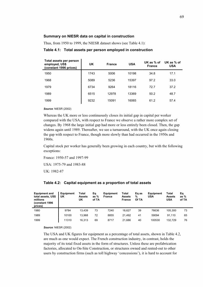
69

Summary on NIESR data on capital in construction

Thus, from 1950 to 1999, the NIESR dataset shows (see Table 4.1):

Table 4.1: Total assets per person employed in construction

Total assets per person employed, US$ (constant 1996 prices)

UK France USA UK as % of France

UK as % of USA

1950 1743 5006 10198 34.8 17.1

1968 5089 5236 15397 97.2 33.0

1979 6734 9264 18116 72.7 37.2

1989 6515 12978 13369 50.2 48.7

1999 9232 15091 16065 61.2 57.4

Source: NIESR (2002)

Whereas the UK more or less continuously closes its initial gap in capital per worker compared with the USA, with respect to France we observe a rather more complex set of changes. By 1968 the large initial gap had more or less entirely been closed. Then, the gap widens again until 1989. Thereafter, we see a turnaround, with the UK once again closing the gap with respect to France, though more slowly than had occurred in the 1950s and 1960s.

Capital stock per worker has generally been growing in each country, but with the following exceptions:

France: 1950-57 and 1997-99

USA: 1975-79 and 1983-88

UK: 1982-87

Table 4.2: Capital equipment as a proportion of total assets

Equipment and total assets, US$ millions (constant 1996 prices)

Equipment UK

Total Assets UK

Eq as % of TA

Equipment France

Total Assets France

Eq as % Of TA

Equipment USA

Total Assets USA

Eq as % of TA

1980 9784 13,439 73 7240 18,627 39 76636 105,300 73

1989 10100 13,968 72 8855 21,492 41 59094 91,110 65

1999 11310 16,313 69 8717 21,686 40 100530 132,729 76

Source: NIESR (2002)

The USA and UK figures for equipment as a percentage of total assets, shown in Table 4.2, are much as one would expect. The French construction industry, in contrast, holds the majority of its total fixed assets in the form of structures. Unless these are prefabrication factories, allocated to On-Site Construction, or structures owned and rented-out to other users by construction firms (such as toll highway ‘concessions’), it is hard to account for

70

this, since by definition on-site construction occurs in premises (structures that are fixed assets) owned by others (the industries’ clients), requiring only administrative offices and depots, for storing equipment and some materials, to be owned by construction firms.

Capital equipment per person employed is shown in Figure 4.1, below. We see that the UK both started and ended the period with levels of equipment per head very similar to those found in France; and that the UK has substantially reduced the gap between it and the USA in equipment per person employed (Fig. 4.1 is in US$ at constant 1996 prices), largely because equipment per worker fell almost by 50% in the USA between 1975 and 1987.

Figure 4.1: Capital equipment per person employed

0

5

10

15

20

1950

1953

1956

1959

1962

1965

1968

1971

1974

1977

1980

1983

1986

1989

1992

1995

1998

$ 00

0s

Germany France UK USA

Source: NIESR (2002) Sectoral Productivity Dataset

Figure 4.2 shows the ratio of the capital stock over the average annual hours worked in construction multiplied by the number of people employed. Both France and the UK show a steady rise in capital intensity since the Second World War in contrast to the United States where the rise in capital per hour worked from 1950 to 1975 was followed by a decline in the ratio until the late 1980s. Once again, this decline in capital per hour worked was caused by the rise in the number of people engaged in construction in the US since 1975 without an equivalent rise in capital to accompany the enlarged workforce.

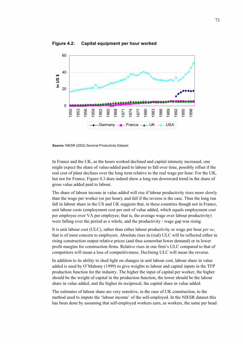
71

Figure 4.2: Capital equipment per hour worked

0

20

40

60

1950

1953

1956

1959

1962

1965

1968

1971

1974

1977

1980

1983

1986

1989

1992

1995

1998

in U

S $

Germany France UK USA

Source: NIESR (2002) Sectoral Productivity Dataset

In France and the UK, as the hours worked declined and capital intensity increased, one might expect the share of value-added paid to labour to fall over time, possibly offset if the real cost of plant declines over the long term relative to the real wage per hour. For the UK, but not for France, Figure 4.3 does indeed show a long run downward trend in the share of gross value added paid to labour.

The share of labour income in value added will rise if labour productivity rises more slowly than the wage per worker (or per hour), and fall if the reverse is the case. Thus the long run fall in labour share in the US and UK suggests that, in these countries though not in France, unit labour costs (employment cost per unit of value added, which equals employment cost per employee over VA per employee; that is, the average wage over labour productivity) were falling over the period as a whole, and the productivity / wage gap was rising.

It is unit labour cost (ULC), rather than either labour productivity or wage per hour per se, that is of most concern to employers. Absolute rises in (real) ULC will be reflected either in rising construction output relative prices (and thus somewhat lower demand) or in lower profit margins for construction firms. Relative rises in one firm’s ULC compared to that of competitors will mean a loss of competitiveness. Declining ULC will mean the reverse.

In addition to its ability to shed light on changes in unit labour cost, labour share in value added is used by O’Mahony (1999) to give weights to labour and capital inputs in the TFP production function for the industry. The higher the input of capital per worker, the higher should be the weight of capital in the production function, the lower should be the labour share in value added, and the higher its reciprocal, the capital share in value added.

The estimates of labour share are very sensitive, in the case of UK construction, to the method used to impute the ‘labour income’ of the self-employed. In the NIESR dataset this has been done by assuming that self-employed workers earn, as workers, the same per head

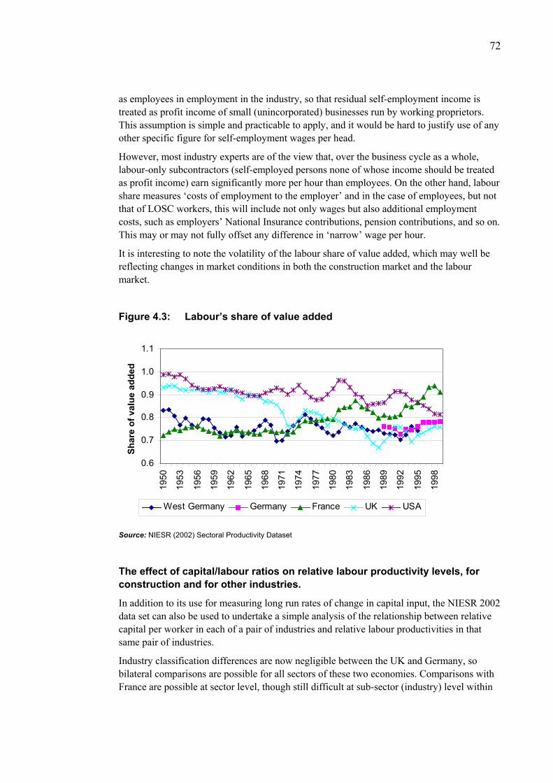
72

as employees in employment in the industry, so that residual self-employment income is treated as profit income of small (unincorporated) businesses run by working proprietors. This assumption is simple and practicable to apply, and it would be hard to justify use of any other specific figure for self-employment wages per head.

However, most industry experts are of the view that, over the business cycle as a whole, labour-only subcontractors (self-employed persons none of whose income should be treated as profit income) earn significantly more per hour than employees. On the other hand, labour share measures ‘costs of employment to the employer’ and in the case of employees, but not that of LOSC workers, this will include not only wages but also additional employment costs, such as employers’ National Insurance contributions, pension contributions, and so on. This may or may not fully offset any difference in ‘narrow’ wage per hour.

It is interesting to note the volatility of the labour share of value added, which may well be reflecting changes in market conditions in both the construction market and the labour market.

Figure 4.3: Labour’s share of value added

0.6

0.7

0.8

0.9

1.0

1.1

1950

1953

1956

1959

1962

1965

1968

1971

1974

1977

1980

1983

1986

1989

1992

1995

1998

Shar

e of

val

ue a

dded

West Germany Germany France UK USA

Source: NIESR (2002) Sectoral Productivity Dataset

The effect of capital/labour ratios on relative labour productivity levels, for construction and for other industries.

In addition to its use for measuring long run rates of change in capital input, the NIESR 2002 data set can also be used to undertake a simple analysis of the relationship between relative capital per worker in each of a pair of industries and relative labour productivities in that same pair of industries.

Industry classification differences are now negligible between the UK and Germany, so bilateral comparisons are possible for all sectors of these two economies. Comparisons with France are possible at sector level, though still difficult at sub-sector (industry) level within

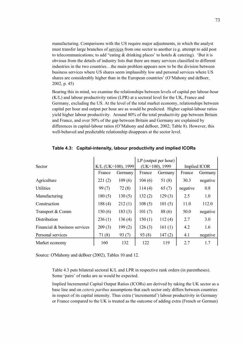
73

manufacturing. Comparisons with the US require major adjustments, in which the analyst must transfer large branches of services from one sector to another (e.g. attempt to add post to telecommunications; to add “eating & drinking places’ to hotels & catering). ‘But it is obvious from the details of industry lists that there are many services classified to different industries in the two countries…the main problem appears now to be the division between business services where US shares seem implausibly low and personal services where US shares are considerably higher than in the European countries’ (O’Mahony and deBoer, 2002, p. 45)

Bearing this in mind, we examine the relationships between levels of capital per labour-hour (K/L) and labour productivity ratios (LPR) at a sectoral level for the UK, France and Germany, excluding the US. At the level of the total market economy, relationships between capital per hour and output per hour are as would be predicted. Higher capital-labour ratios yield higher labour productivity. Around 80% of the total productivity gap between Britain and France, and over 50% of the gap between Britain and Germany are explained by differences in capital-labour ratios (O’Mahony and deBoer, 2002; Table 8). However, this well-behaved and predictable relationship disappears at the sector level.

Table 4.3: Capital-intensity, labour productivity and implied ICORs

SectorFrance Germany France Germany France Germany

Agriculture 221 (2) 109 (6) 104 (6) 51 (8) 30.3 negative

Utilities 99 (7) 72 (8) 114 (4) 65 (7) negative 0.8

Manufacturing 180 (5) 130 (5) 132 (2) 129 (3) 2.5 1.0

Construction 188 (4) 212 (1) 108 (5) 101 (5) 11.0 112.0

Transport & Comm 150 (6) 183 (3) 101 (7) 88 (6) 50.0 negative

Distribution 236 (1) 136 (4) 150 (1) 112 (4) 2.7 3.0

Financial & business services 209 (3) 199 (2) 126 (3) 161 (1) 4.2 1.6

Personal services 71 (8) 93 (7) 93 (8) 147 (2) 4.1 negative

Market economy 160 132 122 119 2.7 1.7

Source: O'Mahony and deBoer (2002), Tables 10 and 12.

K/L (UK=100), 1999LP (output per hour)

(UK=100), 1999 Implied ICOR

Table 4.3 puts bilateral sectoral K/L and LPR in respective rank orders (in parentheses). Some ‘pairs’ of ranks are as would be expected.

Implied Incremental Capital Output Ratios (ICORs) are derived by taking the UK sector as a base line and on ceteris paribus assumptions that each sector only differs between countries in respect of its capital intensity. Thus extra (‘incremental’) labour productivity in Germany or France compared to the UK is treated as the outcome of adding extra (French or German)

74

levels of capital per worker-hour compared to UK levels of capital per hour. The ratio of the ‘extra’ output per hour to the extra capital per hour is described as the ‘implied ICOR’ (removing ‘per labour hour’ from the denominators, the ratio of capital per hour to output per hour becomes the capital-output ratio).

For UK compared to France, Distribution (K/L rank 1; LPR rank 1), Financial & Business services (3; 3) and Personal services (8; 8) show positive relationships between K/L and LP consistent with an implied capital-output ratio broadly similar to that for the whole market economy, of 3 to 1 (an extra 60 units of capital yielding an extra 22 units of output in the case of the French market economy). The implied ICOR for manufacturing is 2.5 to 1.

However, in one sector the sign of the relationship is negative (Gas, Electricity and Water), and in several sectors (including construction) the implied ICORs (incremental capital-output ratios) are very high: agriculture 10 to 1; construction 11 to 1; transport & comm. 50 to 1.

For the UK compared to Germany, Financial & Business services (K/L rank 2; LPR rank 1) and Distribution (4; 4) show positive relationships and implied ICORs in the expected range. Some sectors show positive relationships but very low implied ICORs (GEW, ‘ICOR’ of 0.8; Manufacturing, ‘ICOR’ of 1). Some sectors show negative relationships between relative (Germany to the UK) capital per hour and relative labour productivity (Agriculture, Transport & Comm., Personal Services). Construction shows a positive but very weak relationship, with an implied ICOR of 112.

How should we interpret these findings? One route is to seek sectoral peculiarities in the respective real production functions. However, before we do this it is necessary to note the severe imperfections in the data purporting to measure the input of capital services in the economy at large (capital assets weighted by acquisition price rather than by annual user cost; i.e. a measure of the size of capital stock rather than of the annual flow of capital services) and in those data, crucially for this purpose, purporting to allocate the national capital stock to sectors.

It is relatively unlikely that the systems of national accounts fail to pick up at all significant amounts of capital formation. However, it is much more likely that they allocate it to the ‘wrong’ sector, relative to its actual use. The NIESR 2002 method of measuring capital stocks is based on the Perpetual Inventory Method but using the same assumptions for asset lifespans and depreciation rates in all the countries (in fact, those used in the US national accounts). Thus we can ignore possible failures to pick up asset retirements as an explanation for weak or ‘wrong sign’ relationships. This leaves misattribution of assets to sectors. The basic source of the data (expenditure on purchases of capital assets) identifies owners, who are not necessarily the users of those assets. Whereas, the concept of capital per hour worked refers to assets used by a sector, but not necessarily owned by it. This difference in concept and measure did not matter greatly in an age when the vast majority of capital assets, other than specialist real estate (housing), were owned by their users. Today, in an age of increasingly elaborate forms of financial engineering designed to remove assets and liabilities from the balance sheets of the users of those assets, or simply lease or hire arrangements designed to give greater flexibility and higher rates of asset utilisation, it has become a fundamental problem.

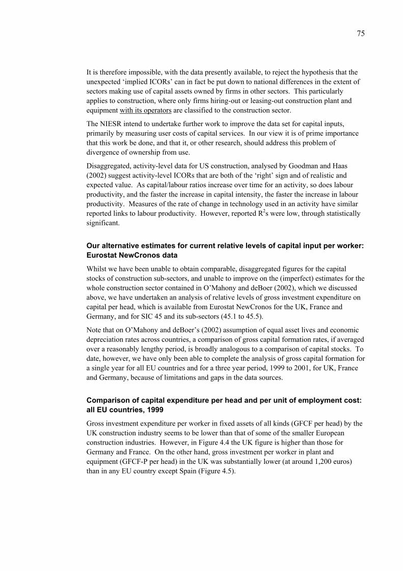
75

It is therefore impossible, with the data presently available, to reject the hypothesis that the unexpected ‘implied ICORs’ can in fact be put down to national differences in the extent of sectors making use of capital assets owned by firms in other sectors. This particularly applies to construction, where only firms hiring-out or leasing-out construction plant and equipment with its operators are classified to the construction sector.

The NIESR intend to undertake further work to improve the data set for capital inputs, primarily by measuring user costs of capital services. In our view it is of prime importance that this work be done, and that it, or other research, should address this problem of divergence of ownership from use.

Disaggregated, activity-level data for US construction, analysed by Goodman and Haas (2002) suggest activity-level ICORs that are both of the ‘right’ sign and of realistic and expected value. As capital/labour ratios increase over time for an activity, so does labour productivity, and the faster the increase in capital intensity, the faster the increase in labour productivity. Measures of the rate of change in technology used in an activity have similar reported links to labour productivity. However, reported R2s were low, through statistically significant.

Our alternative estimates for current relative levels of capital input per worker: Eurostat NewCronos data

Whilst we have been unable to obtain comparable, disaggregated figures for the capital stocks of construction sub-sectors, and unable to improve on the (imperfect) estimates for the whole construction sector contained in O’Mahony and deBoer (2002), which we discussed above, we have undertaken an analysis of relative levels of gross investment expenditure on capital per head, which is available from Eurostat NewCronos for the UK, France and Germany, and for SIC 45 and its sub-sectors (45.1 to 45.5).

Note that on O’Mahony and deBoer’s (2002) assumption of equal asset lives and economic depreciation rates across countries, a comparison of gross capital formation rates, if averaged over a reasonably lengthy period, is broadly analogous to a comparison of capital stocks. To date, however, we have only been able to complete the analysis of gross capital formation for a single year for all EU countries and for a three year period, 1999 to 2001, for UK, France and Germany, because of limitations and gaps in the data sources.

Comparison of capital expenditure per head and per unit of employment cost: all EU countries, 1999

Gross investment expenditure per worker in fixed assets of all kinds (GFCF per head) by the UK construction industry seems to be lower than that of some of the smaller European construction industries. However, in Figure 4.4 the UK figure is higher than those for Germany and France. On the other hand, gross investment per worker in plant and equipment (GFCF-P per head) in the UK was substantially lower (at around 1,200 euros) than in any EU country except Spain (Figure 4.5).

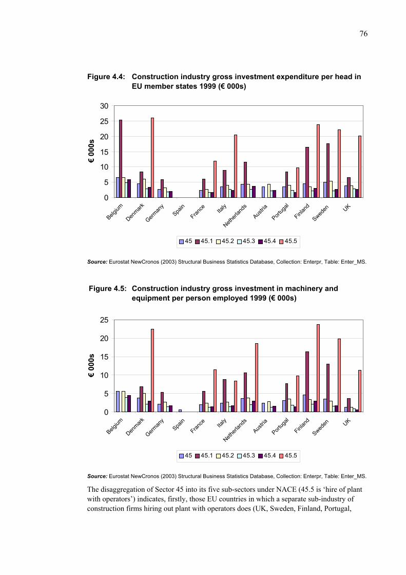
76

Figure 4.4: Construction industry gross investment expenditure per head in EU member states 1999 (€ 000s)

0

5

10

15

20

25

30

Belgium

Denmark

German

ySpa

in

France Ita

ly

Netherl

ands

Austria

Portug

al

Finlan

d

Sweden UK

€ 00

0s

45 45.1 45.2 45.3 45.4 45.5

Source: Eurostat NewCronos (2003) Structural Business Statistics Database, Collection: Enterpr, Table: Enter_MS.

Figure 4.5: Construction industry gross investment in machinery and equipment per person employed 1999 (€ 000s)

0

5

10

15

20

25

Belgium

Denmark

German

ySpa

in

France Ita

ly

Netherl

ands

Austria

Portug

al

Finlan

d

Sweden UK

€ 00

0s

45 45.1 45.2 45.3 45.4 45.5

Source: Eurostat NewCronos (2003) Structural Business Statistics Database, Collection: Enterpr, Table: Enter_MS.

The disaggregation of Sector 45 into its five sub-sectors under NACE (45.5 is ‘hire of plant with operators’) indicates, firstly, those EU countries in which a separate sub-industry of construction firms hiring out plant with operators does (UK, Sweden, Finland, Portugal,

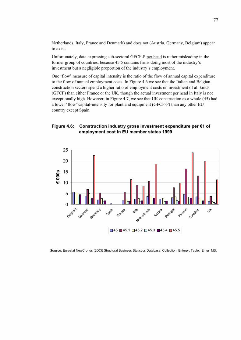
77

Netherlands, Italy, France and Denmark) and does not (Austria, Germany, Belgium) appear to exist.

Unfortunately, data expressing sub-sectoral GFCF-P per head is rather misleading in the former group of countries, because 45.5 contains firms doing most of the industry’s investment but a negligible proportion of the industry’s employment.

One ‘flow’ measure of capital intensity is the ratio of the flow of annual capital expenditure to the flow of annual employment costs. In Figure 4.6 we see that the Italian and Belgian construction sectors spend a higher ratio of employment costs on investment of all kinds (GFCF) than either France or the UK, though the actual investment per head in Italy is not exceptionally high. However, in Figure 4.7, we see that UK construction as a whole (45) had a lower ‘flow’ capital-intensity for plant and equipment (GFCF-P) than any other EU country except Spain.

Figure 4.6: Construction industry gross investment expenditure per €1 of employment cost in EU member states 1999

0

5

10

15

20

25

Belgium

Denmark

German

ySpa

in

France Ita

ly

Netherl

ands

Austria

Portug

al

Finlan

d

Sweden UK

€ 00

0s

45 45.1 45.2 45.3 45.4 45.5

Source: Eurostat NewCronos (2003) Structural Business Statistics Database, Collection: Enterpr, Table: Enter_MS.

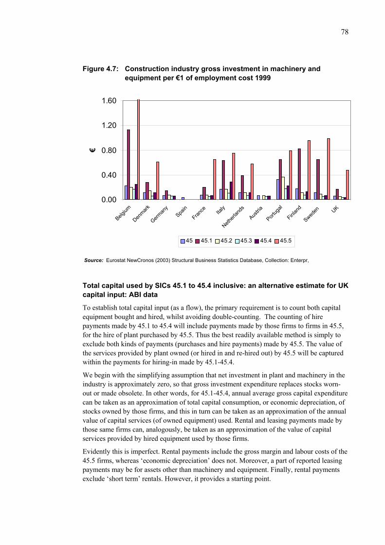
78

Figure 4.7: Construction industry gross investment in machinery and equipment per €1 of employment cost 1999

0.00

0.40

0.80

1.20

1.60

Belgium

Denmark

German

ySpa

in

France Ita

ly

Netherl

ands

Austria

Portug

al

Finlan

d

Sweden UK

€

45 45.1 45.2 45.3 45.4 45.5

Source: Eurostat NewCronos (2003) Structural Business Statistics Database, Collection: Enterpr,

Total capital used by SICs 45.1 to 45.4 inclusive: an alternative estimate for UK capital input: ABI data

To establish total capital input (as a flow), the primary requirement is to count both capital equipment bought and hired, whilst avoiding double-counting. The counting of hire payments made by 45.1 to 45.4 will include payments made by those firms to firms in 45.5, for the hire of plant purchased by 45.5. Thus the best readily available method is simply to exclude both kinds of payments (purchases and hire payments) made by 45.5. The value of the services provided by plant owned (or hired in and re-hired out) by 45.5 will be captured within the payments for hiring-in made by 45.1-45.4.

We begin with the simplifying assumption that net investment in plant and machinery in the industry is approximately zero, so that gross investment expenditure replaces stocks worn-out or made obsolete. In other words, for 45.1-45.4, annual average gross capital expenditure can be taken as an approximation of total capital consumption, or economic depreciation, of stocks owned by those firms, and this in turn can be taken as an approximation of the annual value of capital services (of owned equipment) used. Rental and leasing payments made by those same firms can, analogously, be taken as an approximation of the value of capital services provided by hired equipment used by those firms.

Evidently this is imperfect. Rental payments include the gross margin and labour costs of the 45.5 firms, whereas ‘economic depreciation’ does not. Moreover, a part of reported leasing payments may be for assets other than machinery and equipment. Finally, rental payments exclude ‘short term’ rentals. However, it provides a starting point.

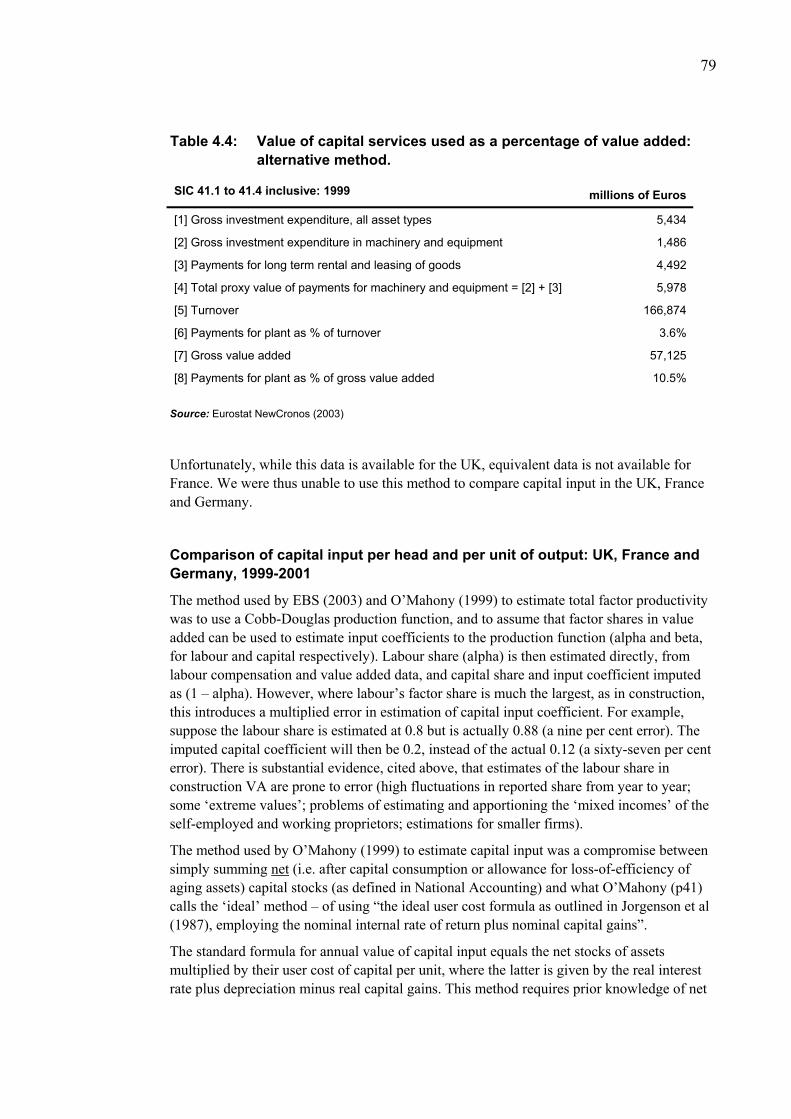
79

Table 4.4: Value of capital services used as a percentage of value added: alternative method.

SIC 41.1 to 41.4 inclusive: 1999 millions of Euros

[1] Gross investment expenditure, all asset types 5,434

[2] Gross investment expenditure in machinery and equipment 1,486

[3] Payments for long term rental and leasing of goods 4,492

[4] Total proxy value of payments for machinery and equipment = [2] + [3] 5,978

[5] Turnover 166,874

[6] Payments for plant as % of turnover 3.6%

[7] Gross value added 57,125

[8] Payments for plant as % of gross value added 10.5%

Source: Eurostat NewCronos (2003)

Unfortunately, while this data is available for the UK, equivalent data is not available for France. We were thus unable to use this method to compare capital input in the UK, France and Germany.

Comparison of capital input per head and per unit of output: UK, France and Germany, 1999-2001

The method used by EBS (2003) and O’Mahony (1999) to estimate total factor productivity was to use a Cobb-Douglas production function, and to assume that factor shares in value added can be used to estimate input coefficients to the production function (alpha and beta, for labour and capital respectively). Labour share (alpha) is then estimated directly, from labour compensation and value added data, and capital share and input coefficient imputed as (1 – alpha). However, where labour’s factor share is much the largest, as in construction, this introduces a multiplied error in estimation of capital input coefficient. For example, suppose the labour share is estimated at 0.8 but is actually 0.88 (a nine per cent error). The imputed capital coefficient will then be 0.2, instead of the actual 0.12 (a sixty-seven per cent error). There is substantial evidence, cited above, that estimates of the labour share in construction VA are prone to error (high fluctuations in reported share from year to year; some ‘extreme values’; problems of estimating and apportioning the ‘mixed incomes’ of the self-employed and working proprietors; estimations for smaller firms).

The method used by O’Mahony (1999) to estimate capital input was a compromise between simply summing net (i.e. after capital consumption or allowance for loss-of-efficiency of aging assets) capital stocks (as defined in National Accounting) and what O’Mahony (p41) calls the ‘ideal’ method – of using “the ideal user cost formula as outlined in Jorgenson et al (1987), employing the nominal internal rate of return plus nominal capital gains”.

The standard formula for annual value of capital input equals the net stocks of assets multiplied by their user cost of capital per unit, where the latter is given by the real interest rate plus depreciation minus real capital gains. This method requires prior knowledge of net

80

stocks, which in turn requires knowledge of asset lives, as well as retirement patterns and the shape and value of relative-efficiency functions over time. Information on actual asset service lives is scarce, and the choice of form chosen for the loss-of-efficiency function is largely a matter of assumption.

Accordingly, we have tried to follow an alternative method for estimating capital input. This is based on decomposing the value of capital services per period into a ‘capital consumption’ and a ‘return on capital’ component; estimating the former; and assuming the latter is similar in each national industry under study.

If we can estimate ‘capital consumption’ as a flow of value added, rather than as a proportion of an (unknown) capital stock, then we can work backwards to estimate the capital stock implied by a given value of capital consumption. We have simply assumed that, on average, capital consumption is just offset by gross capital expenditure, thus maintaining a constant capital stock. We follow Jorgenson et al, but assume that the only capital ‘gains’ are negative, i.e. depreciation.

These assumptions yield a series of ‘pairs’ of possible values for average capital asset lives and for rates of return on capital, in each national industry, that are consistent with any given capital input coefficient in the production function. These can then be judged in terms of plausibility.

We have produced estimates, not of average physical capital stocks per employee, but of capital consumption per employee per year. In principle, this should be proportionate to the average relative ‘user cost’ value of capital services per employee in the construction industries of the three countries for which data was available.

The actual data series we have used is for gross fixed capital expenditure by construction firms, including plant hire firms. We have had simply to assume that the industry is in static long-run equilibrium with respect to its actual capital stock (in terms of efficiency of that stock), so that net investment is on average, over an n-year period, zero. In that case, annual average gross investment expenditure can be taken as a proxy for the value of capital stock used-up (efficiency lost) each year, which should in turn be proportionate to the relative user-cost of capital-services provided by that stock in each country, if we can assume that interest-rates are broadly the same in each country.

[Imagine that all capital equipment, in each country, was rented, without operators, by its user-firms, or by plant-hire-with-operator intermediaries, from owners outside the industry. The annual user-cost of total capital services, V, is the flow of value added that would just enable the financial firms renting-out all this capital equipment to break-even, after allowing for their cost of capital (interest rate plus risk-adjustment) and economic depreciation. Thus, if initial capital stock, K, is 100, economic depreciation is 10, and required return for waiting and risk, r, is 12, then the annual user-cost of the 100 units of K will, in equilibrium, be 22 - the value that leaves a net return of 12 on capital of 100. The relationship is: V = (d.K) + (r.K); where d = 1 / L, and L = average asset life].

Clearly, it is only relative values across countries that can meaningfully be compared using this method, which may yield estimates proportionate to, but not an absolute or cardinal measure of, the value of fixed capital services per period.

81

[This method is an alternative to the theoretical option of taking data for 45.1 to 45.4 only (i.e. excluding 45.5, plant-hire with operators) for gross capital expenditure plus data on payments by them to plant-hire firms. The Eurostat NewCronos database does not in fact contain data on payments for plant hire for France, but only for UK and Germany, thus limiting the value of this option.]

Our source is the Eurostat NewCronos database, which has disaggregated data on total gross capital expenditure and gross capital expenditure on machinery & equipment. Again data availability for UK, France and Germany has restricted the analysis to three years, 1999-2001. Ideally we would have preferred to have data for the whole of a business cycle. Eventually, as new years’ data is added into the NewCronos database, this should become possible. The analysis includes the three European industries but we have been unable to find this sort of disaggregated data for the USA.

The caveats affecting reliability of the NewCronos dataset as a source for labour input apply with much less force to its use as source for capital expenditure, if we can assume that relatively little capital expenditure is actually undertaken by the self-employed, as seems plausible.

This short period for which we have consistent data on gross fixed capital formation makes it impractical, now and in the relevant future, to apply a perpetual-inventory method to estimate capital stocks. Such a measure is useful for dynamic (as opposed to comparative static) studies of the contribution of fixed capital; that is, its contribution to long-run economic growth. Such a method requires a data series for gross fixed capital formation (GFCF), and a derived series for capital consumption, that extend as long as the longest-lived class of capital asset in use by the industry (see: ONS [1998], UK National Accounts: concepts, sources and methods, chapters 4 and 16). It might be worthwhile to explore the possibilities of ‘chaining’ ABI data on GFCF back onto Census of Production data, for the UK construction industry. It seems however that no satisfactory disaggregated long historical series exist for GFCF by the construction industries of France and Germany.

For the ‘mature’ economies under comparison here (UK, France and Germany), we regard slow long-term construction output growth (at ± 0.5% pa) as the relevant ‘stylised fact’ (see, for example, Bon and Crosthwaite, 2000; see also Chapter 3, above). We therefore take the view that it is acceptable to assume a constant long-run capital stock for these industries (no significant long-run capacity-adding ‘accelerator’ or Harrod-Domar effect), subject only to changes in technical knowledge, in rates of ‘catch-up’ with the technical frontier and in relative factor prices.

Using the three-year average of GFCF as a proxy measure of annual capital consumption (as described above) has implications for the interpretation of year-on-year variance of such expenditure. A constant desired capital stock is kept in being by variable annual GFCF if either: the age-profile of the stock is uneven, resulting in uneven values of annual ‘retirements’; or, expected demand levels fluctuate (expectations are revised), so that only over time is the actual stock adjusted to equal the desired stock. With adjustment lags, there may be single years when gross investment is negligible, because, after retirements, actual stock still exceeds desired stock. It may also be that in the short-run, investment expenditure fluctuates in response to immediate past profits. The theoretical approach adopted above has the implication that, for consistency, we do not also try to interpret changes over the n-years

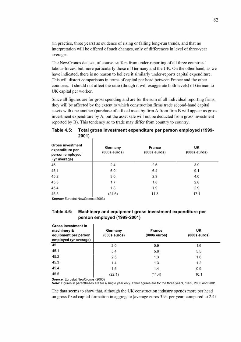
82

(in practice, three years) as evidence of rising or falling long-run trends, and that no interpretation will be offered of such changes, only of differences in level of three-year averages.

The NewCronos dataset, of course, suffers from under-reporting of all three countries’ labour-forces, but more particularly those of Germany and the UK. On the other hand, as we have indicated, there is no reason to believe it similarly under-reports capital expenditure. This will distort comparisons in terms of capital per head between France and the other countries. It should not affect the ratio (though it will exaggerate both levels) of German to UK capital per worker.

Since all figures are for gross spending and are for the sum of all individual reporting firms, they will be affected by the extent to which construction firms trade second-hand capital assets with one another (purchase of a fixed asset by firm A from firm B will appear as gross investment expenditure by A, but the asset sale will not be deducted from gross investment reported by B). This tendency so to trade may differ from country to country.

Table 4.5: Total gross investment expenditure per person employed (1999-2001)

Gross investment expenditure per person employed (yr average)

Germany (000s euros)

France (000s euros)

UK (000s euros)

45 2.4 2.6 3.9 45.1 6.0 6.4 9.1 45.2 3.0 2.9 4.0 45.3 1.7 1.8 2.8 45.4 1.8 1.9 2.9 45.5 (24.6) 11.3 17.1 Source: Eurostat NewCronos (2003)

Table 4.6: Machinery and equipment gross investment expenditure per person employed (1999-2001)

Gross investment in machinery & equipment per person employed (yr average)

Germany (000s euros)

France (000s euros)

UK (000s euros)

45 2.0 0.9 1.6 45.1 5.4 5.6 5.5 45.2 2.5 1.3 1.6 45.3 1.4 1.3 1.2 45.4 1.5 1.4 0.9 45.5 (22.1) (11.4) 10.1 Source: Eurostat NewCronos (2003) Note: Figures in parentheses are for a single year only. Other figures are for the three years, 1999, 2000 and 2001.

The data seems to show that, although the UK construction industry spends more per head on gross fixed capital formation in aggregate (average euros 3.9k per year, compared to 2.4k

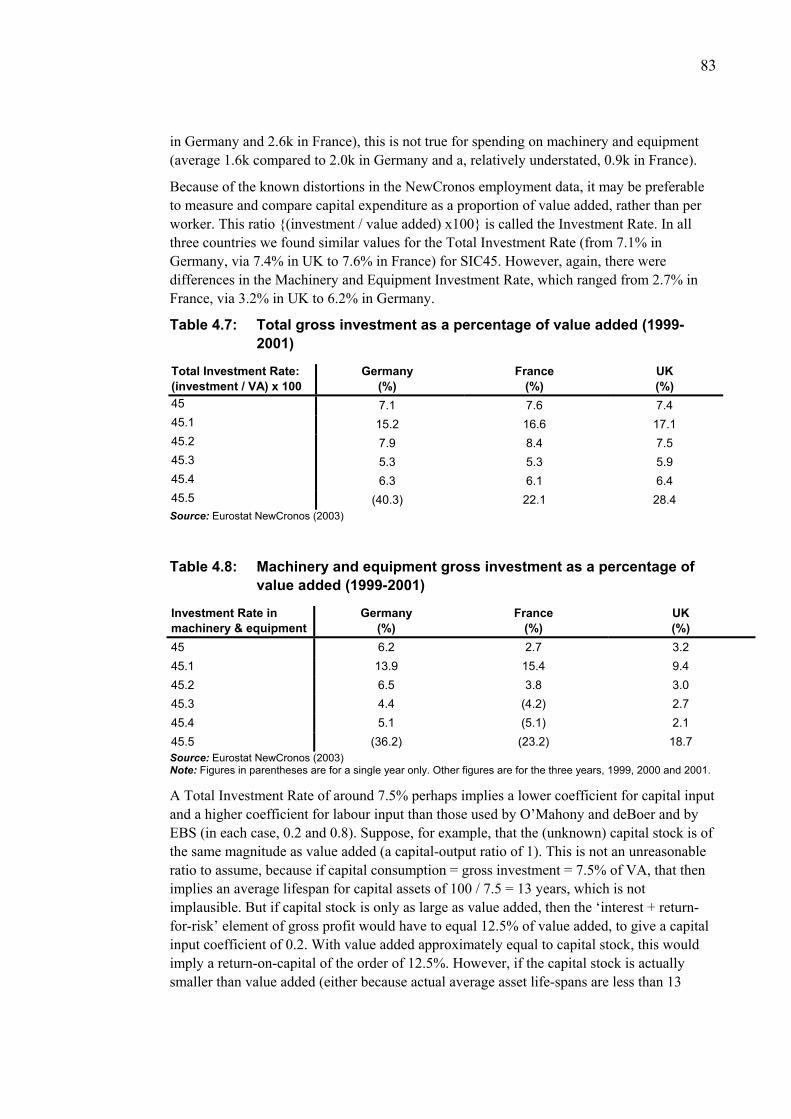
83

in Germany and 2.6k in France), this is not true for spending on machinery and equipment (average 1.6k compared to 2.0k in Germany and a, relatively understated, 0.9k in France).

Because of the known distortions in the NewCronos employment data, it may be preferable to measure and compare capital expenditure as a proportion of value added, rather than per worker. This ratio {(investment / value added) x100} is called the Investment Rate. In all three countries we found similar values for the Total Investment Rate (from 7.1% in Germany, via 7.4% in UK to 7.6% in France) for SIC45. However, again, there were differences in the Machinery and Equipment Investment Rate, which ranged from 2.7% in France, via 3.2% in UK to 6.2% in Germany.

Table 4.7: Total gross investment as a percentage of value added (1999-2001)

Total Investment Rate: (investment / VA) x 100

Germany (%)

France (%)

UK (%)

45 7.1 7.6 7.4 45.1 15.2 16.6 17.1 45.2 7.9 8.4 7.5 45.3 5.3 5.3 5.9 45.4 6.3 6.1 6.4 45.5 (40.3) 22.1 28.4 Source: Eurostat NewCronos (2003)

Table 4.8: Machinery and equipment gross investment as a percentage of value added (1999-2001)

Investment Rate in machinery & equipment

Germany (%)

France (%)

UK (%)

45 6.2 2.7 3.2 45.1 13.9 15.4 9.4 45.2 6.5 3.8 3.0 45.3 4.4 (4.2) 2.7 45.4 5.1 (5.1) 2.1 45.5 (36.2) (23.2) 18.7 Source: Eurostat NewCronos (2003) Note: Figures in parentheses are for a single year only. Other figures are for the three years, 1999, 2000 and 2001.

A Total Investment Rate of around 7.5% perhaps implies a lower coefficient for capital input and a higher coefficient for labour input than those used by O’Mahony and deBoer and by EBS (in each case, 0.2 and 0.8). Suppose, for example, that the (unknown) capital stock is of the same magnitude as value added (a capital-output ratio of 1). This is not an unreasonable ratio to assume, because if capital consumption = gross investment = 7.5% of VA, that then implies an average lifespan for capital assets of 100 / 7.5 = 13 years, which is not implausible. But if capital stock is only as large as value added, then the ‘interest + return-for-risk’ element of gross profit would have to equal 12.5% of value added, to give a capital input coefficient of 0.2. With value added approximately equal to capital stock, this would imply a return-on-capital of the order of 12.5%. However, if the capital stock is actually smaller than value added (either because actual average asset life-spans are less than 13

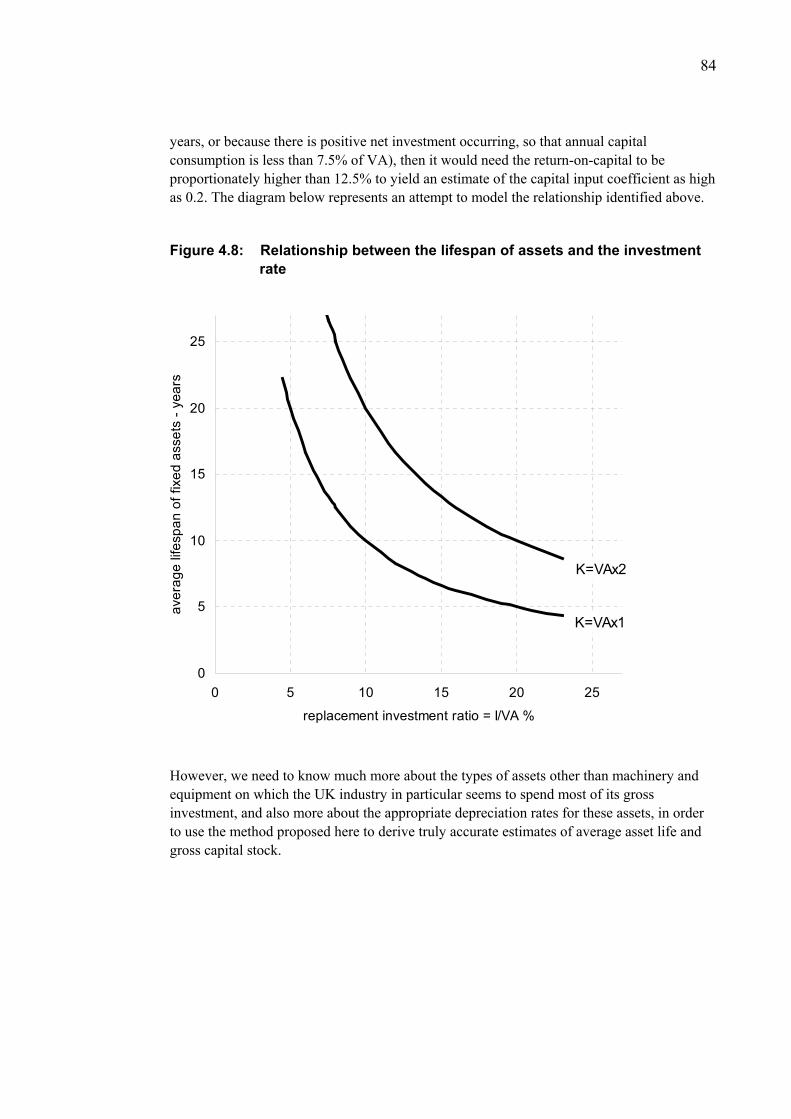
84

years, or because there is positive net investment occurring, so that annual capital consumption is less than 7.5% of VA), then it would need the return-on-capital to be proportionately higher than 12.5% to yield an estimate of the capital input coefficient as high as 0.2. The diagram below represents an attempt to model the relationship identified above.

Figure 4.8: Relationship between the lifespan of assets and the investment rate

0

5

10

15

20

25

0 5 10 15 20 25

replacement investment ratio = I/VA %

aver

age

lifes

pan

of fi

xed

asse

ts -

year

s

K=VAx2

K=VAx1

However, we need to know much more about the types of assets other than machinery and equipment on which the UK industry in particular seems to spend most of its gross investment, and also more about the appropriate depreciation rates for these assets, in order to use the method proposed here to derive truly accurate estimates of average asset life and gross capital stock.

85

5

The UK construction and motor vehicle industries The comparison of construction and motor vehicles manufacturing and repair in this chapter is based on data from 1996 to 2001 taken from the Annual Business Inquiry 2002, supplemented (for some ratios) by data from earlier sources for earlier years. As a critique of the data is given elsewhere, this chapter examines the implications of the published material, used without adjustment. However, it is essential to remember that the ABI data suffers from problems arising both from its exclusion of LOSC self-employed labour and from its treatment of working proprietors (WPs). More specifically, value-added by WPs is included in the value-added figures, but the WPs are not included in the employment figures. It is unclear how much of the value added produced by non-counted LOSCs is included within ABI value added, but it seems likely that some is.

The effect of these measurement problems associated with self-employment is that the ABI seriously overstates actual UK construction labour productivity. This must be borne in mind by the reader throughout this chapter, especially where it deals with apparent relative levels of productivity between construction and vehicles industries.

We begin with a general discussion of the performance of the new construction and vehicle manufacturing industries since 1980. This is followed by a comparison, for 1996-2001, of all construction with MVPR (motor vehicle production and repair) in aggregate and its two constituent parts (SIC 34 and 50.2), beginning with examination of data on labour inputs, followed by investment and ending with a discussion on productivity.

Comparison of the new construction and vehicles manufacturing industries

New construction (about half of the output of SIC 45, ‘the construction industry’) and motor vehicle production (SIC 34) (‘the vehicles manufacturing industry’) are sensible to compare because both are ‘assembly’ industries.

SIC 34 comprises three sub-industries: 34.1 Manufacture of motor vehicles 34.2 Manufacture of motor vehicle bodies 34.3 Manufacture of parts, accessories for motor vehicles

A full comparison of the whole value-chains behind these two (construction and vehicles) respective (largely sub-assembly and assembly) sets of activities would be a major undertaking, completely beyond the scope of this study.

The SIC 34 data on the ratio of value added to turnover shows this to be now only 20% – see below. Moreover, by dividing ABI ‘turnover’ for the whole of industry 34 (£39174m) by number of vehicles produced (1,685,238) [Motor Vehicle Production Inquiry] we can see that the implied ‘turnover per vehicle produced’ in 2001 was £23,245. This is not unrealistic as an approximation of average selling price of a finished vehicle. Thus SIC 34.3 cannot in fact include most of the integrated chain of firms manufacturing parts used in motor vehicle production. No such ‘value chain’ comparison is attempted, and nothing is said here about the respective productivities of the many materials and component manufacturing industries that lie behind the respective final assembly industries.

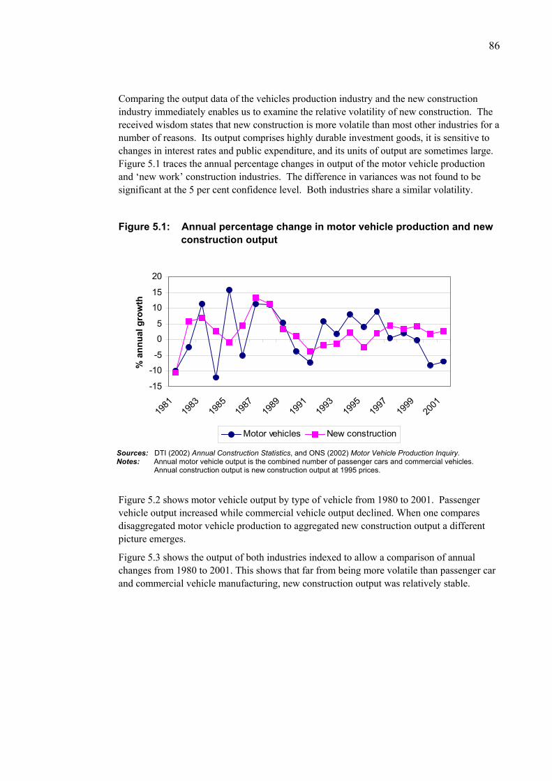
86

Comparing the output data of the vehicles production industry and the new construction industry immediately enables us to examine the relative volatility of new construction. The received wisdom states that new construction is more volatile than most other industries for a number of reasons. Its output comprises highly durable investment goods, it is sensitive to changes in interest rates and public expenditure, and its units of output are sometimes large. Figure 5.1 traces the annual percentage changes in output of the motor vehicle production and ‘new work’ construction industries. The difference in variances was not found to be significant at the 5 per cent confidence level. Both industries share a similar volatility.

Figure 5.1: Annual percentage change in motor vehicle production and new construction output

-15

-10

-5

0

5

10

15

20

1981

1983

1985

1987

1989

1991

1993

1995

1997

1999

2001

% a

nnua

l gro

wth

Motor vehicles New construction

Sources: DTI (2002) Annual Construction Statistics, and ONS (2002) Motor Vehicle Production Inquiry. Notes: Annual motor vehicle output is the combined number of passenger cars and commercial vehicles. Annual construction output is new construction output at 1995 prices.

Figure 5.2 shows motor vehicle output by type of vehicle from 1980 to 2001. Passenger vehicle output increased while commercial vehicle output declined. When one compares disaggregated motor vehicle production to aggregated new construction output a different picture emerges.

Figure 5.3 shows the output of both industries indexed to allow a comparison of annual changes from 1980 to 2001. This shows that far from being more volatile than passenger car and commercial vehicle manufacturing, new construction output was relatively stable.

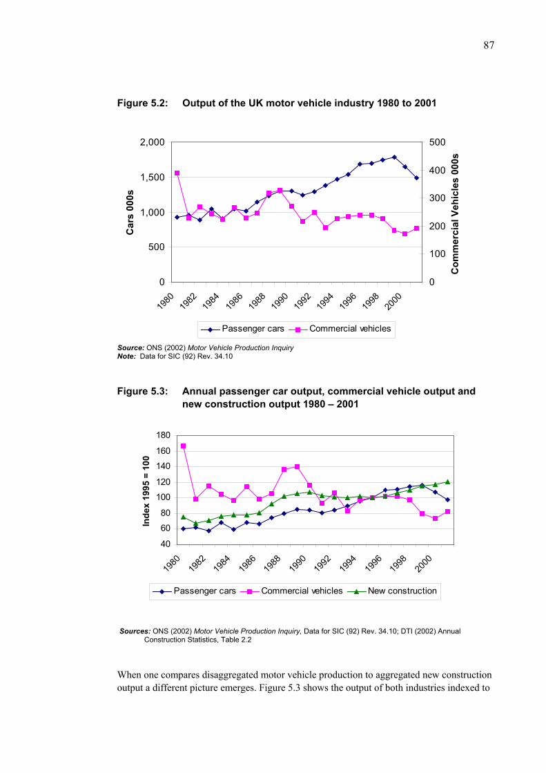
87

Figure 5.2: Output of the UK motor vehicle industry 1980 to 2001

0

500

1,000

1,500

2,000

1980

1982

1984

1986

1988

1990

1992

1994

1996

1998

2000

Car

s 00

0s

0

100

200

300

400

500

Com

mer

cial

Veh

icle

s 00

0s

Passenger cars Commercial vehicles

Source: ONS (2002) Motor Vehicle Production Inquiry Note: Data for SIC (92) Rev. 34.10

Figure 5.3: Annual passenger car output, commercial vehicle output and new construction output 1980 – 2001

40

60

80

100

120

140

160

180

1980

1982

1984

1986

1988

1990

1992

1994

1996

1998

2000

Inde

x 19

95 =

100

Passenger cars Commercial vehicles New construction

Sources: ONS (2002) Motor Vehicle Production Inquiry, Data for SIC (92) Rev. 34.10; DTI (2002) Annual Construction Statistics, Table 2.2

When one compares disaggregated motor vehicle production to aggregated new construction output a different picture emerges. Figure 5.3 shows the output of both industries indexed to

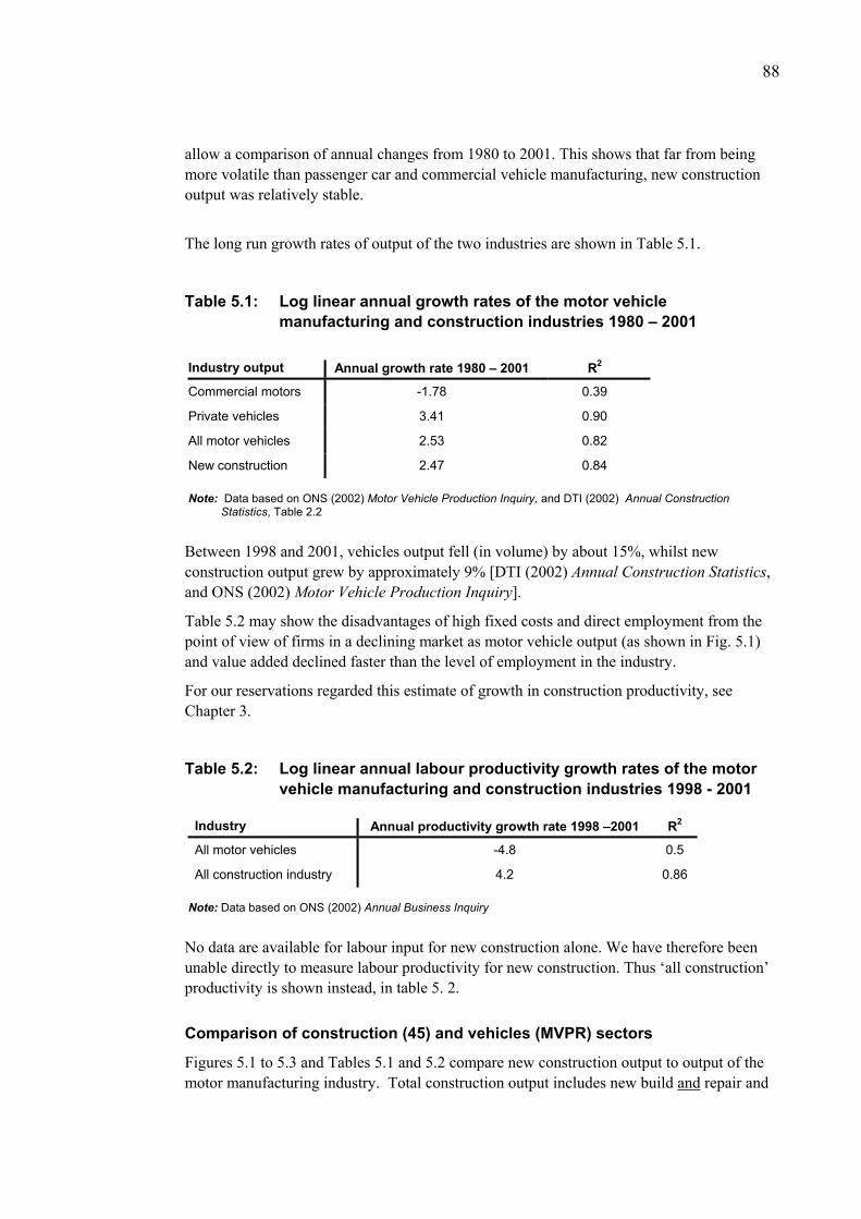
88

allow a comparison of annual changes from 1980 to 2001. This shows that far from being more volatile than passenger car and commercial vehicle manufacturing, new construction output was relatively stable.

The long run growth rates of output of the two industries are shown in Table 5.1.

Table 5.1: Log linear annual growth rates of the motor vehicle manufacturing and construction industries 1980 – 2001

Industry output Annual growth rate 1980 – 2001 R2

Commercial motors -1.78 0.39

Private vehicles 3.41 0.90

All motor vehicles 2.53 0.82

New construction 2.47 0.84

Note: Data based on ONS (2002) Motor Vehicle Production Inquiry, and DTI (2002) Annual Construction Statistics, Table 2.2

Between 1998 and 2001, vehicles output fell (in volume) by about 15%, whilst new construction output grew by approximately 9% [DTI (2002) Annual Construction Statistics, and ONS (2002) Motor Vehicle Production Inquiry].

Table 5.2 may show the disadvantages of high fixed costs and direct employment from the point of view of firms in a declining market as motor vehicle output (as shown in Fig. 5.1) and value added declined faster than the level of employment in the industry.

For our reservations regarded this estimate of growth in construction productivity, see Chapter 3.

Table 5.2: Log linear annual labour productivity growth rates of the motor vehicle manufacturing and construction industries 1998 - 2001

Industry Annual productivity growth rate 1998 –2001 R2

All motor vehicles -4.8 0.5

All construction industry 4.2 0.86 Note: Data based on ONS (2002) Annual Business Inquiry

No data are available for labour input for new construction alone. We have therefore been unable directly to measure labour productivity for new construction. Thus ‘all construction’ productivity is shown instead, in table 5. 2.

Comparison of construction (45) and vehicles (MVPR) sectors

Figures 5.1 to 5.3 and Tables 5.1 and 5.2 compare new construction output to output of the motor manufacturing industry. Total construction output includes new build and repair and

89

maintenance, whereas vehicle manufacturing is only equivalent to new build. We now attempt to allow for that by defining and measuring a Motor Vehicles Production and Repair (MVPR) sector, which can more appropriately be compared to the whole construction industry.

Definition of MVPR sector

Table 5.3 gives an indication of the distribution of vehicle repair and maintenance activity across various service industries (corresponding to 3-digit SIC codes). Table 5.3 shows that, for example, the retail distributors industry had greater workshop receipts than the repairs and servicing industry in 1994. This means that the repairs and servicing industry does not account for even half of repair and maintenance activity in the motor trades.

‘Workshop’ sales essentially represent mainly value added (see note 3 to Table 5.3). They are certainly the nearest equivalent ‘sales’ measure to construction industry R&M value added. For some purposes (comparison of outputs), therefore, the total of the column headed ‘Workshop’ is the most useful figure.

However, employment and other data for vehicle R&M is only available by industry, not by activity. Therefore, the best that can be done, for productivity comparison purposes, is to take SIC industry 50.2 (‘Repairs and servicing’) as representative of this activity. The other four 3-digit parts of SIC 50 predominantly engage in retailing, though with repair and maintenance as a significant secondary activity. Therefore they cannot properly be included in their entirety in a comparison with SIC 45 (construction).

However, their exclusion results in too-low a relative weight being given to R&M as against new production in the calculation of an ‘average’ productivity of the motor vehicles sector as a whole (MVPR), and thus has the effect of raising that apparent average.

Thus total value added of 50.2 in 2001 was only around half that of SIC 34, giving a 2:1 ratio of ‘new production’ to R&M for vehicles. Inclusion of value added in R&M activities in the other sub-industries within SIC 50 would certainly raise this ratio to be much closer to the 1:1 ratio of construction (gross) R&M and new outputs.

Table 5.3: Analysis of motor trades sales and receipts in 1994 (£m)

All (1) Parts (2) Workshop (3) Bonuses (4)

All motor trades 21941 16032 4504 1405

Retail distributors 9914 6637 2498 778

Wholesale distributors 6665 5920 451 294

Repairs and servicing 4993 3245 1438 310

Petrol filling stations 370 230 117 22 Source: ONS (1996) SDA 27 Results of the 1994 Motor Trades Survey, Table 6, p.18

(1) All other motor trades sales and receipts (incl. parts and accessories, repair and servicing, campaign bonuses and caravans (2) Sales of parts and accessories (incl. those used in repair and servicing work) (3) Workshop receipts (excl. parts and accessories) (4) All other motor trades sales (incl. bonuses and caravans)

90

Note also that, though the sum of columns 2 and 3 in Table 5.3 (‘parts’ plus ‘workshop’) is the nearest we have to an equivalent of construction R&M ‘output’ (in the sense that term is used in the DTI construction statistics), it is far from being an exact equivalent because it includes a considerable value of sales of parts for DIY use.

Thus, although vehicle manufacturing has sometimes been compared to the construction industry, we believe that a better comparison of the two sectors can be made by including repair and maintenance of motor vehicles. This makes sense because both sectors involve the production of durable goods that require maintenance. The construction sector data (SIC 45) includes a very large element of repair and maintenance whereas the vehicles sector is divided between motor vehicle manufacturing (SIC 34) and a service industry (SIC 50) comprising sub-industries engaged in activities including both vehicle retailing and vehicle repair & maintenance. For reasons described above, in the rest of this chapter the vehicles sector is represented by the combination of SIC 34 and SIC 50.2, to form motor vehicle production and repair (MVPR).

Labour intensity and unit labour cost

Investment decisions by firms, and hence the labour intensity of the production process, are influenced by the cost of employment per person. Figure 5.4 shows (according to ABI data) the cost of employment per person in the construction and MVPR sectors. As expected the cost of employment per person in construction is less than the cost of employment per person in motor vehicle production, but more than in vehicles repair and servicing, leaving it lower overall. This difference or gap narrowed substantially between 1998 and 2001, as employment cost per head fell in SIC 34, but rose in both SIC 50.2 and 45.

We must however draw attention to the low level of the figures reported in the ABI for construction industry and vehicle repair industry employment cost per head. In our view they are too low, in absolute terms, to be plausibly accurate, unless part-time employment is prevalent in either industry (a substantial recent reduction in average hours worked per person per year in SIC 34 might explain some of the recent reported decline in its productivity per person per year). Certainly, part-time employment is not widespread in the construction industry, for which the ABI estimate of employment cost per head is lower than the level implied by alternative sources (National Accounts for labour income and LFS for number of workers; or New Earnings Survey). Again the WP problem identified earlier (page 56) affects vehicle repair as well as construction.

Employment cost over turnover may be used as a rough-and-ready measure of unit labour cost. [We ordinarily prefer for this purpose, and use below, labour share in value added. However, there are particular problems affecting the ABI data for both labour share in value added and employment cost share in turnover.] In Figure 5.5 the proportion of employment costs to sales is shown as just below 20 per cent in construction compared to approximately 15 per cent in the MVPR industry.

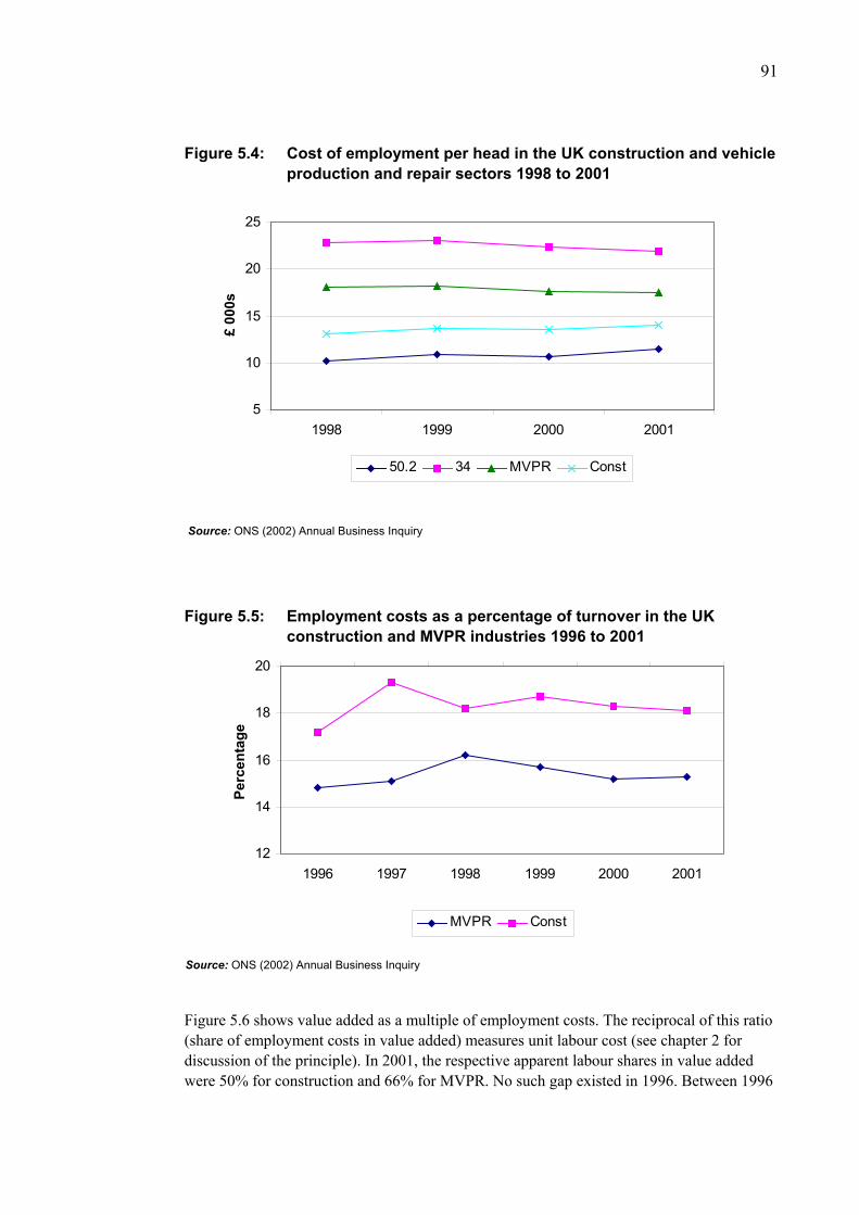
91

Figure 5.4: Cost of employment per head in the UK construction and vehicle production and repair sectors 1998 to 2001

5

10

15

20

25

1998 1999 2000 2001

£ 00

0s

50.2 34 MVPR Const

Source: ONS (2002) Annual Business Inquiry

Figure 5.5: Employment costs as a percentage of turnover in the UK construction and MVPR industries 1996 to 2001

12

14

16

18

20

1996 1997 1998 1999 2000 2001

Perc

enta

ge

MVPR Const

Source: ONS (2002) Annual Business Inquiry

Figure 5.6 shows value added as a multiple of employment costs. The reciprocal of this ratio (share of employment costs in value added) measures unit labour cost (see chapter 2 for discussion of the principle). In 2001, the respective apparent labour shares in value added were 50% for construction and 66% for MVPR. No such gap existed in 1996. Between 1996

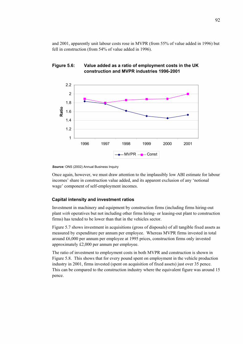
92

and 2001, apparently unit labour costs rose in MVPR (from 55% of value added in 1996) but fell in construction (from 54% of value added in 1996).

Figure 5.6: Value added as a ratio of employment costs in the UK construction and MVPR industries 1996-2001

1

1.2

1.4

1.6

1.8

2

2.2

1996 1997 1998 1999 2000 2001

Rat

io

MVPR Const

Source: ONS (2002) Annual Business Inquiry

Once again, however, we must draw attention to the implausibly low ABI estimate for labour incomes’ share in construction value added, and its apparent exclusion of any ‘notional wage’ component of self-employment incomes.

Capital intensity and investment ratios

Investment in machinery and equipment by construction firms (including firms hiring-out plant with operatives but not including other firms hiring- or leasing-out plant to construction firms) has tended to be lower than that in the vehicles sector.

Figure 5.7 shows investment in acquisitions (gross of disposals) of all tangible fixed assets as measured by expenditure per annum per employee. Whereas MVPR firms invested in total around £6,000 per annum per employee at 1995 prices, construction firms only invested approximately £2,000 per annum per employee.

The ratio of investment to employment costs in both MVPR and construction is shown in Figure 5.8. This shows that for every pound spent on employment in the vehicle production industry in 2001, firms invested (spent on acquisition of fixed assets) just over 35 pence. This can be compared to the construction industry where the equivalent figure was around 15 pence.

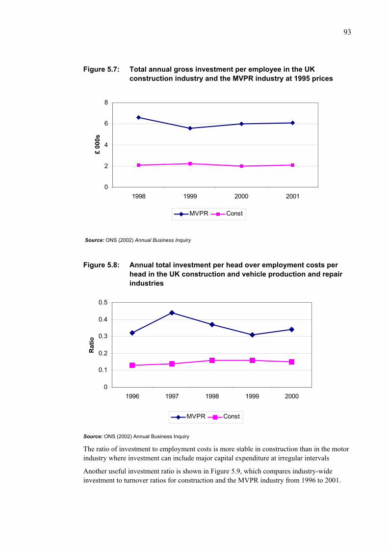
93

Figure 5.7: Total annual gross investment per employee in the UK construction industry and the MVPR industry at 1995 prices

0

2

4

6

8

1998 1999 2000 2001

£ 00

0s

MVPR Const

Source: ONS (2002) Annual Business Inquiry

Figure 5.8: Annual total investment per head over employment costs per head in the UK construction and vehicle production and repair industries

0

0.1

0.2

0.3

0.4

0.5

1996 1997 1998 1999 2000

Rat

io

MVPR Const

Source: ONS (2002) Annual Business Inquiry

The ratio of investment to employment costs is more stable in construction than in the motor industry where investment can include major capital expenditure at irregular intervals

Another useful investment ratio is shown in Figure 5.9, which compares industry-wide investment to turnover ratios for construction and the MVPR industry from 1996 to 2001.

94

As a sector the data shows that MVPR invests a higher proportion of its turnover, between 4 and 6 per cent, than does construction, approximately 2 to 3 per cent. One use of this ratio is to make comparison with net profit margins, the ratio of profit to turnover. If the ratio of the net margin is approximately equal to the investment / turnover ratio, it indicates that an industry is in a position to finance its investment requirements from its profits (whether directly, with no debt or interest but all profits retained; or indirectly, with both distributions of interest from net profits but also new debt consistent with a constant gearing ratio). The construction industry investment / turnover ratio in this sense appears quite high when we consider construction profit margins are often as low as 1 to 3 per cent of turnover.

Nevertheless, the difference in investment / turnover ratios between the motor vehicle industry and construction seems to be related to the fact that the car industry enjoys higher profit margins than construction. As a result a greater proportion of turnover can be used for investment out of the profits generated from any given volume of sales, compared to construction, where profit margins on turnover are among the lowest of any industry. Causality here may, in the long term, run in both directions, and thus be cumulative: higher margins permit the financing of higher investment / turnover ratios, but this investment (now and in the past) permits and generates the higher margins.

Figure 5.9: Ratio of annual investment in acquisitions of fixed assets to turnover in the UK construction and vehicle production and repair industries

0

0.02

0.04

0.06

0.08

1996 1997 1998 1999 2000

Rat

io

MVPR Const

Source: ONS, (2002) Annual Business Inquiry

Overall, the picture that emerges is that the vehicles sector (MVPR) invests more per head and a greater proportion of its turnover and value added than does construction. One would therefore expect the vehicles sector (MVPR) to be more capital intensive (in the strict sense, i.e. a higher value of capital services used per year per unit of labour services) than construction (which it may well be) and therefore to have higher labour productivity.

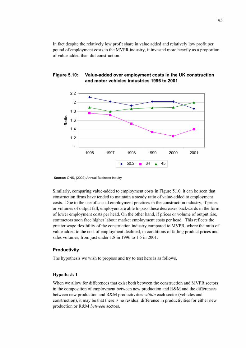
95

In fact despite the relatively low profit share in value added and relatively low profit per pound of employment costs in the MVPR industry, it invested more heavily as a proportion of value added than did construction.

Figure 5.10: Value-added over employment costs in the UK construction and motor vehicles industries 1996 to 2001

1

1.2

1.4

1.6

1.8

2

2.2

1996 1997 1998 1999 2000 2001

Rat

io

50.2 34 45

Source: ONS, (2002) Annual Business Inquiry

Similarly, comparing value-added to employment costs in Figure 5.10, it can be seen that construction firms have tended to maintain a steady ratio of value-added to employment costs. Due to the use of casual employment practices in the construction industry, if prices or volumes of output fall, employers are able to pass these decreases backwards in the form of lower employment costs per head. On the other hand, if prices or volume of output rise, contractors soon face higher labour market employment costs per head. This reflects the greater wage flexibility of the construction industry compared to MVPR, where the ratio of value added to the cost of employment declined, in conditions of falling product prices and sales volumes, from just under 1.8 in 1996 to 1.5 in 2001.

Productivity

The hypothesis we wish to propose and try to test here is as follows.

Hypothesis 1

When we allow for differences that exist both between the construction and MVPR sectors in the composition of employment between new production and R&M and the differences between new production and R&M productivities within each sector (vehicles and construction), it may be that there is no residual difference in productivities for either new production or R&M between sectors.

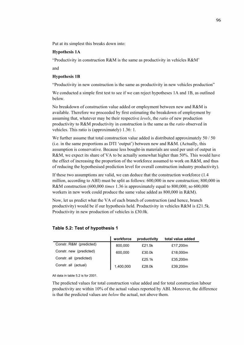
96

Put at its simplest this breaks down into:

Hypothesis 1A

“Productivity in construction R&M is the same as productivity in vehicles R&M’

and

Hypothesis 1B

“Productivity in new construction is the same as productivity in new vehicles production”

We conducted a simple first test to see if we can reject hypotheses 1A and 1B, as outlined below.

No breakdown of construction value added or employment between new and R&M is available. Therefore we proceeded by first estimating the breakdown of employment by assuming that, whatever may be their respective levels, the ratio of new production productivity to R&M productivity in construction is the same as the ratio observed in vehicles. This ratio is (approximately) 1.36: 1.

We further assume that total construction value added is distributed approximately 50 / 50 (i.e. in the same proportions as DTI ‘output’) between new and R&M. (Actually, this assumption is conservative. Because less bought-in materials are used per unit of output in R&M, we expect its share of VA to be actually somewhat higher than 50%. This would have the effect of increasing the proportion of the workforce assumed to work on R&M, and thus of reducing the hypothesised prediction level for overall construction industry productivity).

If these two assumptions are valid, we can deduce that the construction workforce (1.4 million, according to ABI) must be split as follows: 600,000 in new construction; 800,000 in R&M construction (600,000 times 1.36 is approximately equal to 800,000; so 600,000 workers in new work could produce the same value added as 800,000 in R&M).

Now, let us predict what the VA of each branch of construction (and hence, branch productivity) would be if our hypothesis held. Productivity in vehicles R&M is £21.5k. Productivity in new production of vehicles is £30.0k.

Table 5.2: Test of hypothesis 1

workforce productivity total value added Constr. R&M (predicted) 800,000 £21.5k £17,200m Constr. new (predicted) 600,000 £30.0k £18,000m Constr. all (predicted) £25.1k £35,200m Constr. all (actual) 1,400,000 £28.0k £39,200m

All data in table 5.2 is for 2001.

The predicted values for total construction value added and for total construction labour productivity are within 10% of the actual values reported by ABI. Moreover, the difference is that the predicted values are below the actual, not above them.

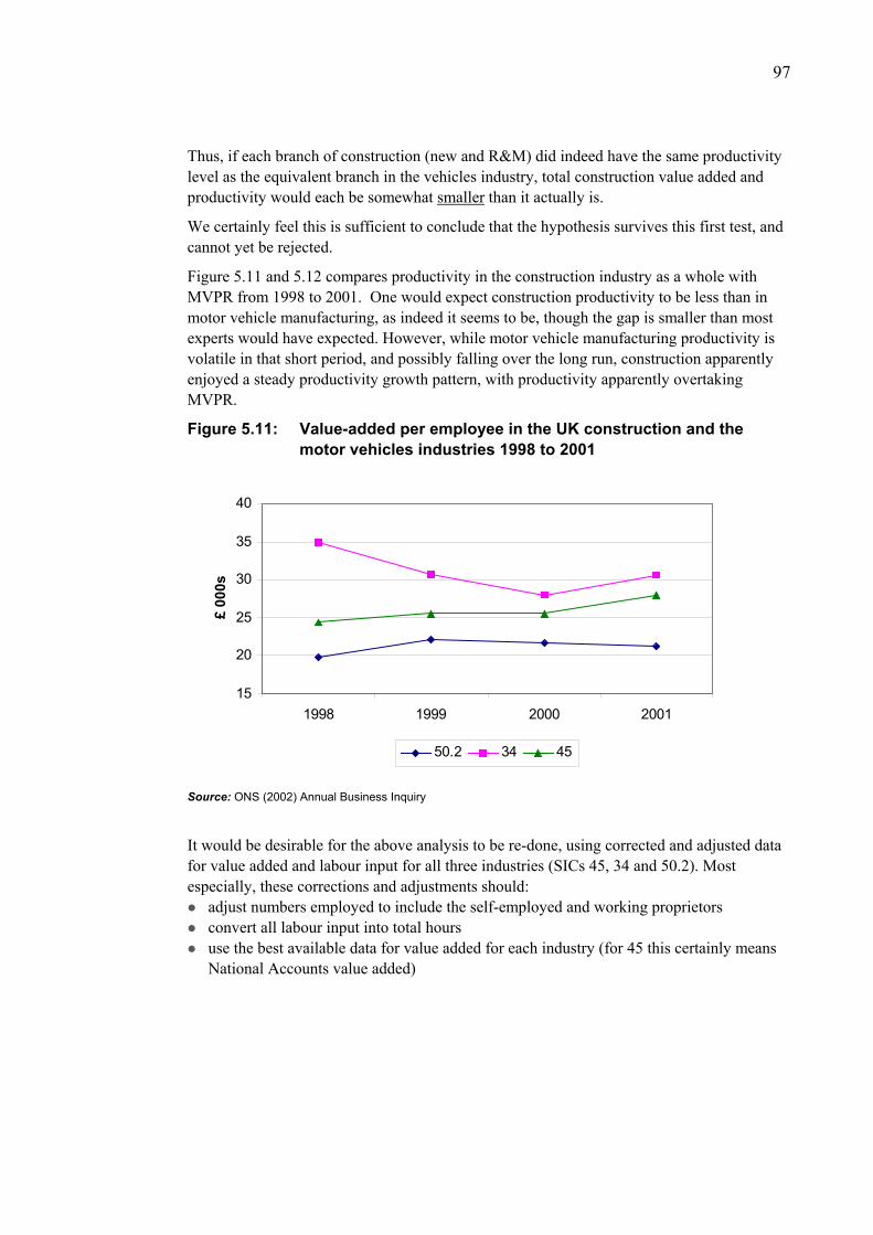
97

Thus, if each branch of construction (new and R&M) did indeed have the same productivity level as the equivalent branch in the vehicles industry, total construction value added and productivity would each be somewhat smaller than it actually is.

We certainly feel this is sufficient to conclude that the hypothesis survives this first test, and cannot yet be rejected.

Figure 5.11 and 5.12 compares productivity in the construction industry as a whole with MVPR from 1998 to 2001. One would expect construction productivity to be less than in motor vehicle manufacturing, as indeed it seems to be, though the gap is smaller than most experts would have expected. However, while motor vehicle manufacturing productivity is volatile in that short period, and possibly falling over the long run, construction apparently enjoyed a steady productivity growth pattern, with productivity apparently overtaking MVPR.

Figure 5.11: Value-added per employee in the UK construction and the motor vehicles industries 1998 to 2001

15

20

25

30

35

40

1998 1999 2000 2001

£ 00

0s

50.2 34 45

Source: ONS (2002) Annual Business Inquiry

It would be desirable for the above analysis to be re-done, using corrected and adjusted data for value added and labour input for all three industries (SICs 45, 34 and 50.2). Most especially, these corrections and adjustments should:

adjust numbers employed to include the self-employed and working proprietors

convert all labour input into total hours use the best available data for value added for each industry (for 45 this certainly means National Accounts value added)

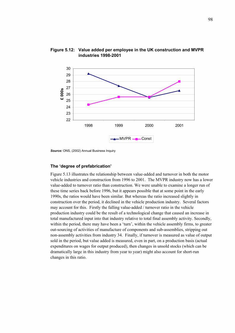
98

Figure 5.12: Value added per employee in the UK construction and MVPR industries 1998-2001

22

2324

2526

27

2829

30

1998 1999 2000 2001

£ 00

0s

MVPR Const

Source: ONS, (2002) Annual Business Inquiry

The ‘degree of prefabrication’

Figure 5.13 illustrates the relationship between value-added and turnover in both the motor vehicle industries and construction from 1996 to 2001. The MVPR industry now has a lower value-added to turnover ratio than construction. We were unable to examine a longer run of these time series back before 1996, but it appears possible that at some point in the early 1990s, the ratios would have been similar. But whereas the ratio increased slightly in construction over the period, it declined in the vehicle production industry. Several factors may account for this. Firstly the falling value-added / turnover ratio in the vehicle production industry could be the result of a technological change that caused an increase in total manufactured input into that industry relative to total final assembly activity. Secondly, within the period, there may have been a ‘turn’, within the vehicle assembly firms, to greater out-sourcing of activities of manufacture of components and sub-assemblies, stripping out non-assembly activities from industry 34. Finally, if turnover is measured as value of output sold in the period, but value added is measured, even in part, on a production basis (actual expenditures on wages for output produced), then changes in unsold stocks (which can be dramatically large in this industry from year to year) might also account for short-run changes in this ratio.

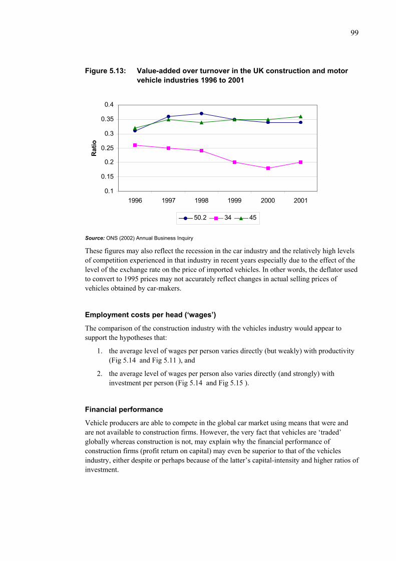
99

Figure 5.13: Value-added over turnover in the UK construction and motor vehicle industries 1996 to 2001

0.1

0.15

0.2

0.25

0.3

0.35

0.4

1996 1997 1998 1999 2000 2001

Rat

io

50.2 34 45

Source: ONS (2002) Annual Business Inquiry

These figures may also reflect the recession in the car industry and the relatively high levels of competition experienced in that industry in recent years especially due to the effect of the level of the exchange rate on the price of imported vehicles. In other words, the deflator used to convert to 1995 prices may not accurately reflect changes in actual selling prices of vehicles obtained by car-makers.

Employment costs per head (‘wages’)

The comparison of the construction industry with the vehicles industry would appear to support the hypotheses that:

1. the average level of wages per person varies directly (but weakly) with productivity (Fig 5.14 and Fig 5.11 ), and

2. the average level of wages per person also varies directly (and strongly) with investment per person (Fig 5.14 and Fig 5.15 ).

Financial performance

Vehicle producers are able to compete in the global car market using means that were and are not available to construction firms. However, the very fact that vehicles are ‘traded’ globally whereas construction is not, may explain why the financial performance of construction firms (profit return on capital) may even be superior to that of the vehicles industry, either despite or perhaps because of the latter’s capital-intensity and higher ratios of investment.

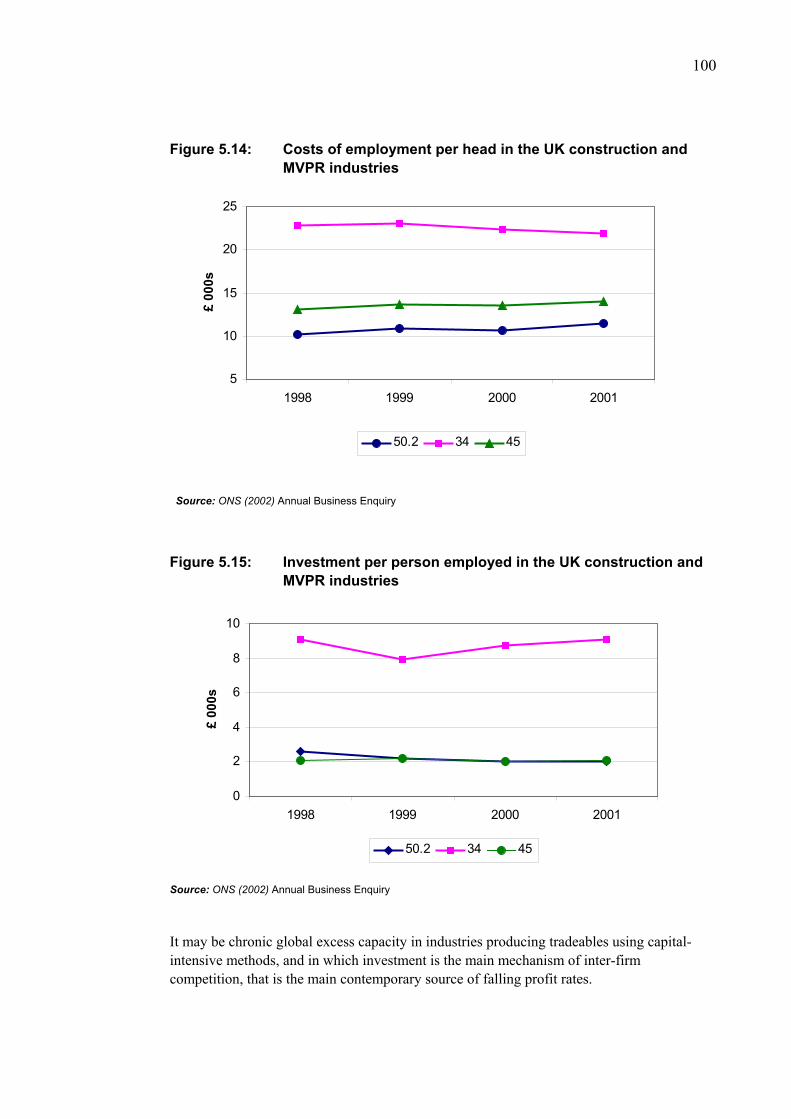
100

Figure 5.14: Costs of employment per head in the UK construction and MVPR industries

5

10

15

20

25

1998 1999 2000 2001

£ 00

0s

50.2 34 45

Source: ONS (2002) Annual Business Enquiry

Figure 5.15: Investment per person employed in the UK construction and MVPR industries

0

2

4

6

8

10

1998 1999 2000 2001

£ 00

0s

50.2 34 45

Source: ONS (2002) Annual Business Enquiry

It may be chronic global excess capacity in industries producing tradeables using capital-intensive methods, and in which investment is the main mechanism of inter-firm competition, that is the main contemporary source of falling profit rates.

101

The ‘best of both worlds’, for construction, would be to experience an equivalent stimulus to productivity to that given by global competition, but without the depressing effect on capacity utilisation and profit rates that follows from that same globalisation.

Summary

The most striking findings from this comparison would appear to be:

1. that the much higher levels of capital per worker found in SIC 34 compared to new construction, yield it only a modest labour productivity advantage over new construction.

2. that construction R&M activity may have higher, or at least comparable, productivity than vehicles R&M activity.

3. that new construction activity may have higher, or at least comparable, total factor productivity than vehicles production.

102

6 Summary addressing the terms of reference

Introduction

Our terms of reference were to produce best estimates, including descriptions of methodologies used, for the following within the constraints/limits of the currently available data:

Estimates of average labour productivity levels in different sectors of construction in the UK, France, Germany and the USA;

Estimates of recent trends in annual growth rates of labour productivity in different sectors of the four countries’ construction industries; Estimates of average physical capital stocks per employee (or employee-hour) in the different sectors of the four countries’ construction industries. Estimates of average labour productivity levels in new and repair & maintenance construction as compared with motor vehicle manufacturing and repair

It was envisaged at commissioning that this would be done for the UK, France and Germany using the Eurostat NewCronos dataset, to give results for the five sub-sectors of construction defined by NACE, 45.1 to 45.5; and that the authors would investigate the possibilities of finding and converting US sub-sectoral data to make it comparable with NACE 3-digit sub sectors. In course of executing the research, it became clear that:

We had no fully satisfactory whole-sector (all construction) baselines for either relative levels or rates of growth of labour productivities on which to draw The Eurostat NewCronos data, based on the ABI and its European counterparts, was too seriously flawed to be the basis for a sub-sectoral comparison of relative productivity levels, and could only with major caveats be used even for a comparison of sub-sectoral rates of change in productivities The statistics would not support any sub-sectoral measurement of gross capital investment and capital consumption by the four national construction industries on a consistent and comparable basis over a sufficiently long period to apply a Perpetual Inventory Method to yield direct estimates of net capital stocks for the sub-sectors

It also became clear that the NACE 3-digit sub-sectors were not in fact a particularly useful starting-point for an investigation of the differences between productivities in branches of construction, and the contribution these might make to overall levels and rates of growth of construction productivity. In this report, therefore, whilst we have, wherever possible, produced estimates of productivities using the sources and methods originally envisaged, we have had to caution the reader against placing reliance on these estimates, and to outline and / or offer alternative sources and methods.

Therefore the work done has had to ‘begin at the beginning’, and to attempt to develop better solutions for the basic problems of

Measurement of labour input to construction on an internationally comparable basis

103

Appropriate deflators to produce internationally comparable series for output at constant prices

Appropriate purchasing power parities to produce comparable international valuations of output

We believe nonetheless that this report makes a significant contribution to the understanding of the relative productivity performance of the UK, French, German and US construction industries. We have confidence that our final estimates of comparative labour productivity levels and rates of change for the construction industry as a whole are the best produced to date.

We also believe that we have both Demonstrated the sensitivity of our results, and those of others, to critical changes in assumptions and methods; and Identified a set of remaining possible further improvements to the data and further investigations that helps identify an agenda for further research on construction productivity measurement

Average labour productivity levels in construction

As requested we have produced single figure estimates for labour productivity (LP) levels (value-added per person) in the construction industry in the UK, France, Germany and the USA. We have done this for 1999 using GDP PPPs and Labour Force Survey (LFS) [Current Population Survey for USA] data, our preferred method. Construction value-added for 1999 was taken from the OECD ‘Annual National Accounts’, to allow comparison with the USA, and equates to gross value-added at basic prices for the UK, France and Germany, and gross value-added at factor cost for the USA (includes indirect taxes), in millions of national currency units (current prices). These were converted to a common base (US $) using 1999 GDP PPPs (OECD, 2000). This was the last triennial benchmark year. The labour input data was obtained from LFS + CPS data reported by the ILO and Eurostat NewCronos. The apparent LP of the four countries’ construction industries is reported in the table below.

Table 6.1: Our estimates of relative levels of labour productivity, per person-year

1999 VA ($m) LFS (000's) LP ($000's) Ratios of LP

(UK=100)

France 56056 1444 38.8 119

Germany 103200 3148 32.8 101

UK 63871 1961 32.6 100

USA 417300 8987 46.4 142

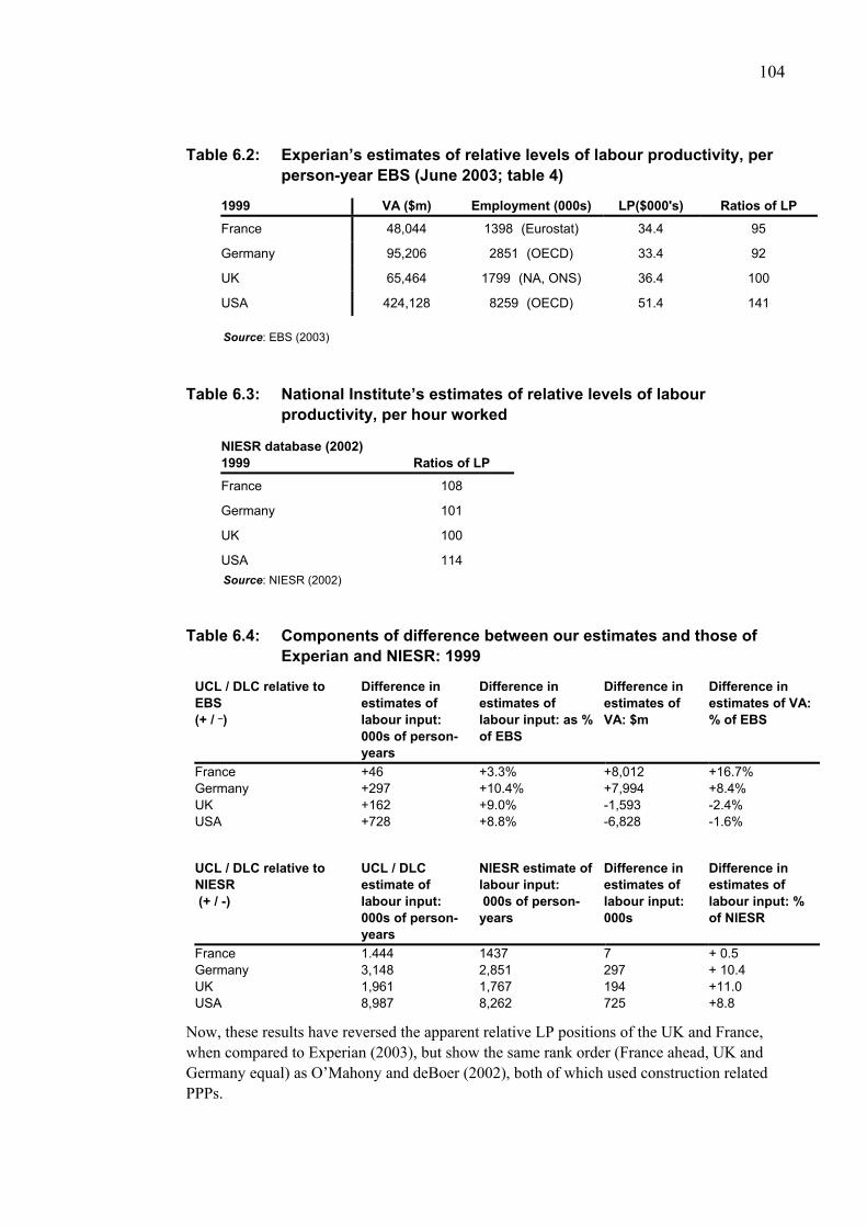
104

Table 6.2: Experian’s estimates of relative levels of labour productivity, per person-year EBS (June 2003; table 4)

1999 VA ($m) Employment (000s) LP($000's) Ratios of LP

France 48,044 1398 (Eurostat) 34.4 95

Germany 95,206 2851 (OECD) 33.4 92

UK 65,464 1799 (NA, ONS) 36.4 100

USA 424,128 8259 (OECD) 51.4 141

Source: EBS (2003)

Table 6.3: National Institute’s estimates of relative levels of labour productivity, per hour worked

NIESR database (2002) 1999

Ratios of LP

France 108

Germany 101

UK 100

USA 114 Source: NIESR (2002)

Table 6.4: Components of difference between our estimates and those of Experian and NIESR: 1999

UCL / DLC relative to EBS (+ / _)

Difference in estimates of labour input: 000s of person-years

Difference in estimates of labour input: as % of EBS

Difference in estimates of VA: $m

Difference in estimates of VA: % of EBS

France +46 +3.3% +8,012 +16.7% Germany +297 +10.4% +7,994 +8.4% UK +162 +9.0% -1,593 -2.4% USA +728 +8.8% -6,828 -1.6%

UCL / DLC relative to NIESR (+ / -)

UCL / DLC estimate of labour input: 000s of person-years

NIESR estimate of labour input: 000s of person-years

Difference in estimates of labour input: 000s

Difference in estimates of labour input: % of NIESR

France 1.444 1437 7 + 0.5 Germany 3,148 2,851 297 + 10.4 UK 1,961 1,767 194 +11.0 USA 8,987 8,262 725 +8.8

Now, these results have reversed the apparent relative LP positions of the UK and France, when compared to Experian (2003), but show the same rank order (France ahead, UK and Germany equal) as O’Mahony and deBoer (2002), both of which used construction related PPPs.

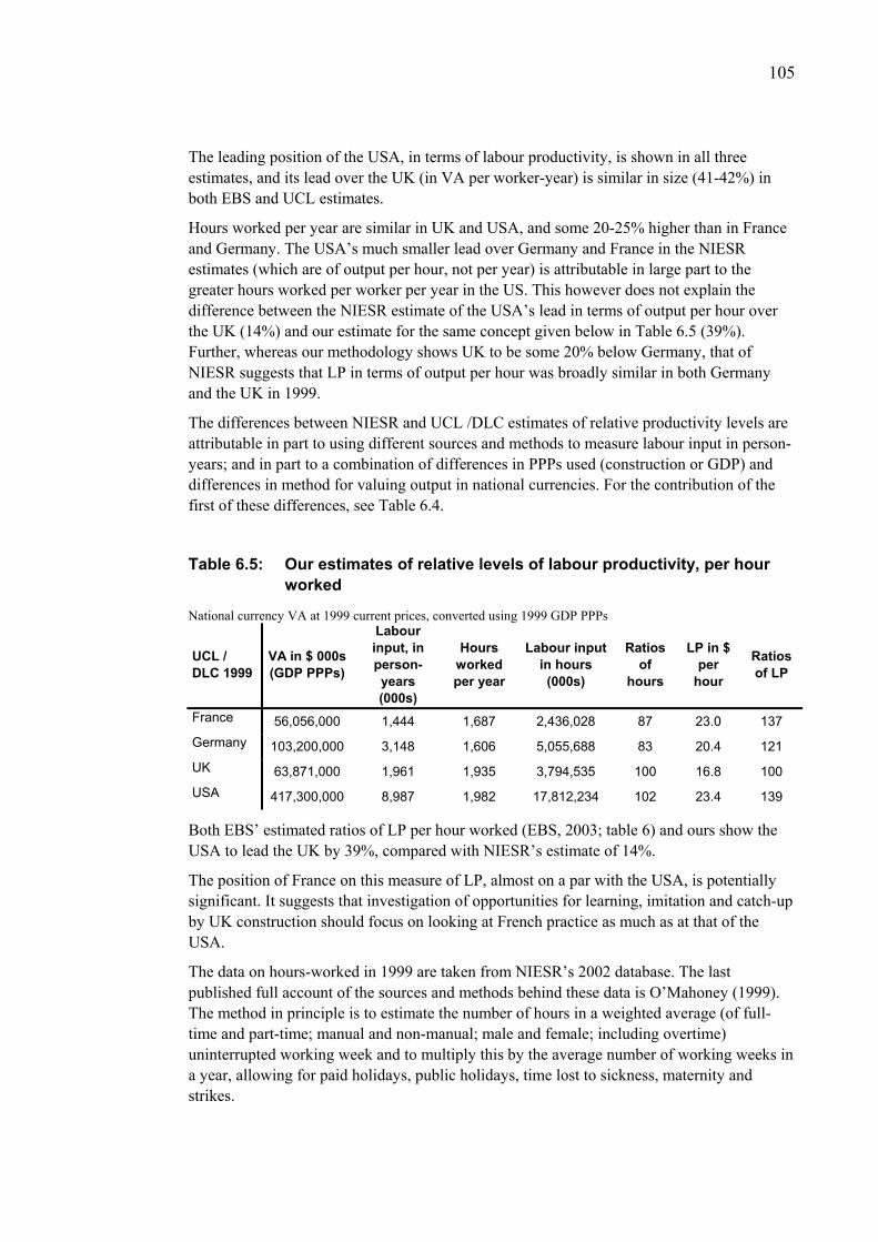
105

The leading position of the USA, in terms of labour productivity, is shown in all three estimates, and its lead over the UK (in VA per worker-year) is similar in size (41-42%) in both EBS and UCL estimates.

Hours worked per year are similar in UK and USA, and some 20-25% higher than in France and Germany. The USA’s much smaller lead over Germany and France in the NIESR estimates (which are of output per hour, not per year) is attributable in large part to the greater hours worked per worker per year in the US. This however does not explain the difference between the NIESR estimate of the USA’s lead in terms of output per hour over the UK (14%) and our estimate for the same concept given below in Table 6.5 (39%). Further, whereas our methodology shows UK to be some 20% below Germany, that of NIESR suggests that LP in terms of output per hour was broadly similar in both Germany and the UK in 1999.

The differences between NIESR and UCL /DLC estimates of relative productivity levels are attributable in part to using different sources and methods to measure labour input in person-years; and in part to a combination of differences in PPPs used (construction or GDP) and differences in method for valuing output in national currencies. For the contribution of the first of these differences, see Table 6.4.

Table 6.5: Our estimates of relative levels of labour productivity, per hour worked

National currency VA at 1999 current prices, converted using 1999 GDP PPPs

UCL / DLC 1999

VA in $ 000s (GDP PPPs)

Labour input, in person-years (000s)

Hours worked per year

Labour input in hours (000s)

Ratios of

hours

LP in $ per

hour

Ratios of LP

France 56,056,000 1,444 1,687 2,436,028 87 23.0 137 Germany 103,200,000 3,148 1,606 5,055,688 83 20.4 121 UK 63,871,000 1,961 1,935 3,794,535 100 16.8 100 USA 417,300,000 8,987 1,982 17,812,234 102 23.4 139

Both EBS’ estimated ratios of LP per hour worked (EBS, 2003; table 6) and ours show the USA to lead the UK by 39%, compared with NIESR’s estimate of 14%.

The position of France on this measure of LP, almost on a par with the USA, is potentially significant. It suggests that investigation of opportunities for learning, imitation and catch-up by UK construction should focus on looking at French practice as much as at that of the USA.

The data on hours-worked in 1999 are taken from NIESR’s 2002 database. The last published full account of the sources and methods behind these data is O’Mahoney (1999). The method in principle is to estimate the number of hours in a weighted average (of full-time and part-time; manual and non-manual; male and female; including overtime) uninterrupted working week and to multiply this by the average number of working weeks in a year, allowing for paid holidays, public holidays, time lost to sickness, maternity and strikes.

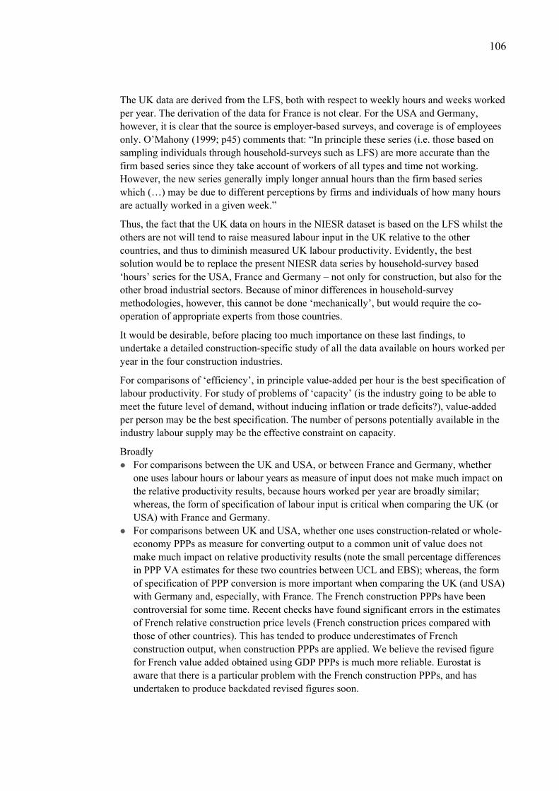
106

The UK data are derived from the LFS, both with respect to weekly hours and weeks worked per year. The derivation of the data for France is not clear. For the USA and Germany, however, it is clear that the source is employer-based surveys, and coverage is of employees only. O’Mahony (1999; p45) comments that: “In principle these series (i.e. those based on sampling individuals through household-surveys such as LFS) are more accurate than the firm based series since they take account of workers of all types and time not working. However, the new series generally imply longer annual hours than the firm based series which (…) may be due to different perceptions by firms and individuals of how many hours are actually worked in a given week.”

Thus, the fact that the UK data on hours in the NIESR dataset is based on the LFS whilst the others are not will tend to raise measured labour input in the UK relative to the other countries, and thus to diminish measured UK labour productivity. Evidently, the best solution would be to replace the present NIESR data series by household-survey based ‘hours’ series for the USA, France and Germany – not only for construction, but also for the other broad industrial sectors. Because of minor differences in household-survey methodologies, however, this cannot be done ‘mechanically’, but would require the co-operation of appropriate experts from those countries.

It would be desirable, before placing too much importance on these last findings, to undertake a detailed construction-specific study of all the data available on hours worked per year in the four construction industries.

For comparisons of ‘efficiency’, in principle value-added per hour is the best specification of labour productivity. For study of problems of ‘capacity’ (is the industry going to be able to meet the future level of demand, without inducing inflation or trade deficits?), value-added per person may be the best specification. The number of persons potentially available in the industry labour supply may be the effective constraint on capacity.

Broadly For comparisons between the UK and USA, or between France and Germany, whether one uses labour hours or labour years as measure of input does not make much impact on the relative productivity results, because hours worked per year are broadly similar; whereas, the form of specification of labour input is critical when comparing the UK (or USA) with France and Germany.

For comparisons between UK and USA, whether one uses construction-related or whole-economy PPPs as measure for converting output to a common unit of value does not make much impact on relative productivity results (note the small percentage differences in PPP VA estimates for these two countries between UCL and EBS); whereas, the form of specification of PPP conversion is more important when comparing the UK (and USA) with Germany and, especially, with France. The French construction PPPs have been controversial for some time. Recent checks have found significant errors in the estimates of French relative construction price levels (French construction prices compared with those of other countries). This has tended to produce underestimates of French construction output, when construction PPPs are applied. We believe the revised figure for French value added obtained using GDP PPPs is much more reliable. Eurostat is aware that there is a particular problem with the French construction PPPs, and has undertaken to produce backdated revised figures soon.

107

For comparisons between USA and Germany, whether one uses household-survey data, on the one hand, or OECD figures on the other, for the size of the labour force does not make much impact on the relative productivity results (in both countries the [LFS and CPS] household survey shows a labour force some 8 to 10% larger than the OECD figures, which are derived by making adjustments to employer-survey-derived data for employees).

However, the OECD figure for the UK labour-force is an obvious serious understatement (it measures only employees, with no self-employment adjustment). For this reason, the OECD figure was not used by EBS. The difference between the OECD and UCL estimates for 2000 is very large (1.32m as compared to 1.92m). The reason the difference between UCL and EBS estimates is much smaller (for 1999, 162000; 1.96m as against 1.80m) is that, for the UK only, EBS chose not to use OECD, but to take their estimate from the ONS ‘Blue Book’ (National Accounts), which is itself partially adjusted to reflect the LFS data (it is based on LFS for its estimate of self-employment, and DTI’s employer-based survey for its estimate of employees). Because of the extent of self-employment in UK construction, it obviously has an enormous impact on relative productivity results if a measure of labour-force is used that only captures employees. For comparisons of France with the UK, USA and Germany, it makes a significant impact on relative productivity results if one uses OECD (or Eurostat) data for labour-force rather than household-survey based data. This is simply because, for France but for none of the other countries, the OECD reports LFS-based estimates of the labour-force. Thus OECD-derived comparisons of France with the other three countries are not like-for-like. For Germany (by 300,000), UK (by 600,000) and USA (by 800,000), OECD reports figures for labour-force that are much smaller than the household-survey figures. For France, Eurostat reports a labour-force just slightly below the LFS figure (a difference of only 64,000 workers in 2000), whereas for the other two European countries, the Eurostat figure is much smaller than the LFS figure (a difference of 500,000 for Germany and 600,000 for the UK). Switching from OECD (or Eurostat) to LFS-derived estimates for labour forces significantly increases the measured size of the labour-force in the other three countries (a fortiori, in the UK), but not, of course, in France. Much of France’s higher placement in the ‘UCL league table’ compared to the ‘EBS league table’ is attributable to this. For comparisons of the UK with Germany and the USA, it makes little impact on relative productivity results whether one uses EBS’s hybrid-data (Blue Book for UK, OECD for Germany and USA) or household-survey data. In each country, the latter is some 8 to 10% larger than the former. For comparisons of levels of LP between UK construction and other UK industries (such as vehicles), it is important to recognize that, for those other industries, LFS data on labour input will not normally be available. Because the LFS delivers an estimate of the labour force in construction some 9% bigger than the next-highest set of multi-industry estimates (the Blue Book), its use will tend to depress relative construction productivity in comparison with other industries. Use of ABI data for this purpose, on the other hand, suffers the opposite problem (see chapter 5). Single-year comparisons of relative LP levels are highly sensitive to the choice of year. This is especially so when comparing UK or USA with France or Germany. See Table 6.13, below. There are wide fluctuations from year to year in French and German LP,

108

simply because, in these countries, year-on-year change in labour input is lagged about one year behind change in value added. Disaggregated data on LP are not available on a comparable basis for the US. For the remaining three countries, only in Germany did we find significant differences in level of LP between the NACE sub-sectors 45.2, 45.3 and 45.4 (the sub-sectors that employ over 90% of the total workforce). There would seem therefore to be limited value in pursuing further disaggregated studies of relative productivity using the NACE categories. However, differences in labour productivity by output-type (new construction compared to R&M; civil engineering compared to building) are probably more significant, and should be the focus of any further disaggregated investigation or proposals to improve data collection.

Recent trends in annual growth rates of labour productivity in construction

[A] From Eurostat data, derived from ABI and its foreign equivalents

We have produced estimates of short-period rates of change in LP in different sectors (45.1 to 45.5) of the three European countries’ construction industries including time series of LP for the various sub-sectors of construction. However we have been unable to find this kind of data for the USA. The source used for this was the Eurostat NewCronos database (data is in €s at current prices). Data availability has restricted the analysis to 3 years, namely 1999-2001, thus meaningful trends are impossible to identify at present, although the data provides a starting point and will become more useful if it continues to be collected on a consistent basis.

It is essential to note that this data must not be used for comparison of levels (say, of LP levels in 45.1 or 45.2 in UK and in France or Germany). For the reasons discussed above, the Eurostat data seriously overstates UK construction labour productivity compared to that of Germany and, above all, France. What is true for the aggregate (SIC 45) is of course true for its components, which simply sum to the reported weighted mean.

Because the reported rates of change in LP (taken from Eurostat) exclude a large, and potentially variable (see Table 6.7, below), proportion of the actual labour force in Germany and the UK (though are much more nearly ‘complete’ in coverage for France) then, even if their value added numerators are accurate, it follows that the unreliable denominators mean that we must be extremely cautious in using this source even to measure rates of change in LP.

Table 6.6: Alternative estimates of labour force: European Labour Force Surveys and Eurostat from Employer Surveys

Number employed, in 2000

ELFS (household

survey); 000s

Eurostat NewCronos;

000s

Difference, as % of ELFS

France 1501 1437 -4% Germany 3075 2263 -26% UK 1917 1339 -28%

Source: ILO (2003); Eurostat NewCronos (2003)

109

Table 6.7: Eurostat estimates as percentages of ELFS – 1999, 2000 and 2001 Eurostat as % of ELFS

1999 2000 2001 Range

France 96.8 95.6 95.9 1.2 Germany 72.0 69.9 67.9 4.0 UK 67.6 67.1 66.5 1.1

Source: Eurostat NewCronos (2003)

Recent (i.e. 1999 onwards) Eurostat data for the UK show some, but not all, of the problems we reported on in Chapters 2 and 3. They appear to show, for example, ABI value added converted to euros using exchange rates, i.e. neither construction-based nor GDP-based PPPs have been used.

Thus though we have tried to use Eurostat data for all three countries to maintain a consistent approach, we have very little confidence in the integrity of the data.

Specifically, for the industry as a whole, i.e. SIC 45, Eurostat shows the UK’s LP per person apparently to be growing rapidly over this three-year period (1999, 2000 and 2001) from €44,000 to €56,000 (+ 27%, in current price euros) while LP in France and Germany appears to be relatively stable at around €35,000.

Eurostat data appears to show the same pattern of much faster LP growth in each sub-sector of SIC 45 in UK, compared to France and Germany. Specifically the UK’s LP in each of 45.1 to 45.4 appears, according to Eurostat data, to be growing over the period while LP in France and Germany remained relatively static. The situation for 45.5 is slightly different with LP relatively stable over the period for both France and the UK (only one observation is available for Germany).

However, this 27% increase in apparent current-price UK value added per person employed over just two years seems prima facie implausible, and we advise strongly against attaching undue significance to it.

[B] Our ‘best estimates’: From National Accounts and Household-Survey data.

Direct comparison with our preferred sources of data for the same period reveals the following (Table 6.8):

Table 6.8: Growth of UK labour productivity, 1999-2001

National Accounts VA / LFS labour % change, 1999 to 2001

In PPPs at current prices + 13% at constant 1995 prices + 2% In £ sterling at current prices + 8.5% at constant 1995 prices + 0.5%

Source: OECD (2003); ILO (2003)

110

Given our concerns regarding the Eurostat data we estimated recent trends in growth rates of labour productivity using OECD and LFS data. Now, this data is only available for the aggregate (SIC 45) industry and disaggregation is therefore not possible. However, we believe the value of sub-dividing into SIC 45.1 to 45.5, is negligible given the current state of the data, and for the reasons given above in Section 6.2. Again we followed a similar method to that outlined in the previous section on levels.

Table 6.9: Construction VA at constant 1995 prices (US $m). Converted by us using GDP PPPs (from original constant price series in national currencies in OECD)

1992 1993 1994 1995 1996 1997 1998 1999 2000 2001

France 65752 53439 57228 57917 54749 49547 49356 51504 56746 58358

Germany 104566 102269 110198 110728 105231 108909 106010 107204 107421 99781

UK 51887 49686 50788 50775 52966 55354 54308 54738 55725 58638

USA 257800 264700 281900 284300 300400 308100 331300 349600 359400 353700

Source: OECD (2003)

Table 6.10: Construction labour, in thousands. Labour Force Surveys (from ILO)

1992 1993 1994 1995 1996 1997 1998 1999 2000 2001

France 1666 1521 1476 1514 1516 1465 1427 1444 1503 1520

Germany 2835 2947 3112 3344 3477 3272 3139 3148 3098 2926

UK 1783 1685 1864 1839 1825 1874 1907 1961 1996 2057

USA 7063 7276 7493 7668 7943 8302 8518 8987 9433 9581

Source: ILO (2003)

Table 6.11: Construction labour productivity index (1999 = 100), at constant

1995 prices. Converted to $s using GDP PPPs. Our conversion

1992 1993 1994 1995 1996 1997 1998 1999 2000 2001

France 110 98 109 107 101 95 97 100 106 108

Germany 108 102 104 97 89 98 99 100 102 100

UK 104 106 97 99 104 106 102 100 100 102

USA 94 94 97 95 97 95 100 100 98 95

Source: OECD (2003); ILO (2003)

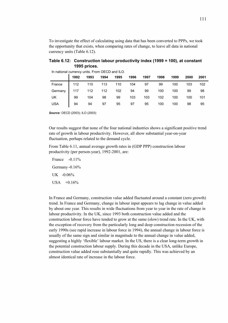
111

To investigate the effect of calculating using data that has been converted to PPPs, we took the opportunity that exists, when comparing rates of change, to leave all data in national currency units (Table 6.12).

Table 6.12: Construction labour productivity index (1999 = 100), at constant 1995 prices.

In national currency units. From OECD and ILO. 1992 1993 1994 1995 1996 1997 1998 1999 2000 2001

France 112 110 113 110 104 97 99 100 103 102

Germany 117 112 112 102 94 99 100 100 99 98

UK 99 104 98 99 103 103 102 100 100 101

USA 94 94 97 95 97 95 100 100 98 95

Source: OECD (2003); ILO (2003)

Our results suggest that none of the four national industries shows a significant positive trend rate of growth in labour productivity. However, all show substantial year-on-year fluctuation, perhaps related to the demand cycle.

From Table 6.11, annual average growth rates in (GDP PPP) construction labour productivity (per person-year), 1992-2001, are:

France -0.11%

Germany -0.16%

UK -0.06%

USA +0.16%

In France and Germany, construction value added fluctuated around a constant (zero growth) trend. In France and Germany, change in labour input appears to lag change in value added by about one year. This results in wide fluctuations from year to year in the rate of change in labour productivity. In the UK, since 1993 both construction value added and the construction labour force have tended to grow at the same (slow) trend rate. In the UK, with the exception of recovery from the particularly long and deep construction recession of the early 1990s (see rapid increase in labour force in 1994), the annual change in labour force is usually of the same sign and similar in magnitude to the annual change in value added, suggesting a highly ‘flexible’ labour market. In the US, there is a clear long-term growth in the potential construction labour supply. During this decade in the USA, unlike Europe, construction value added rose substantially and quite rapidly. This was achieved by an almost identical rate of increase in the labour force.

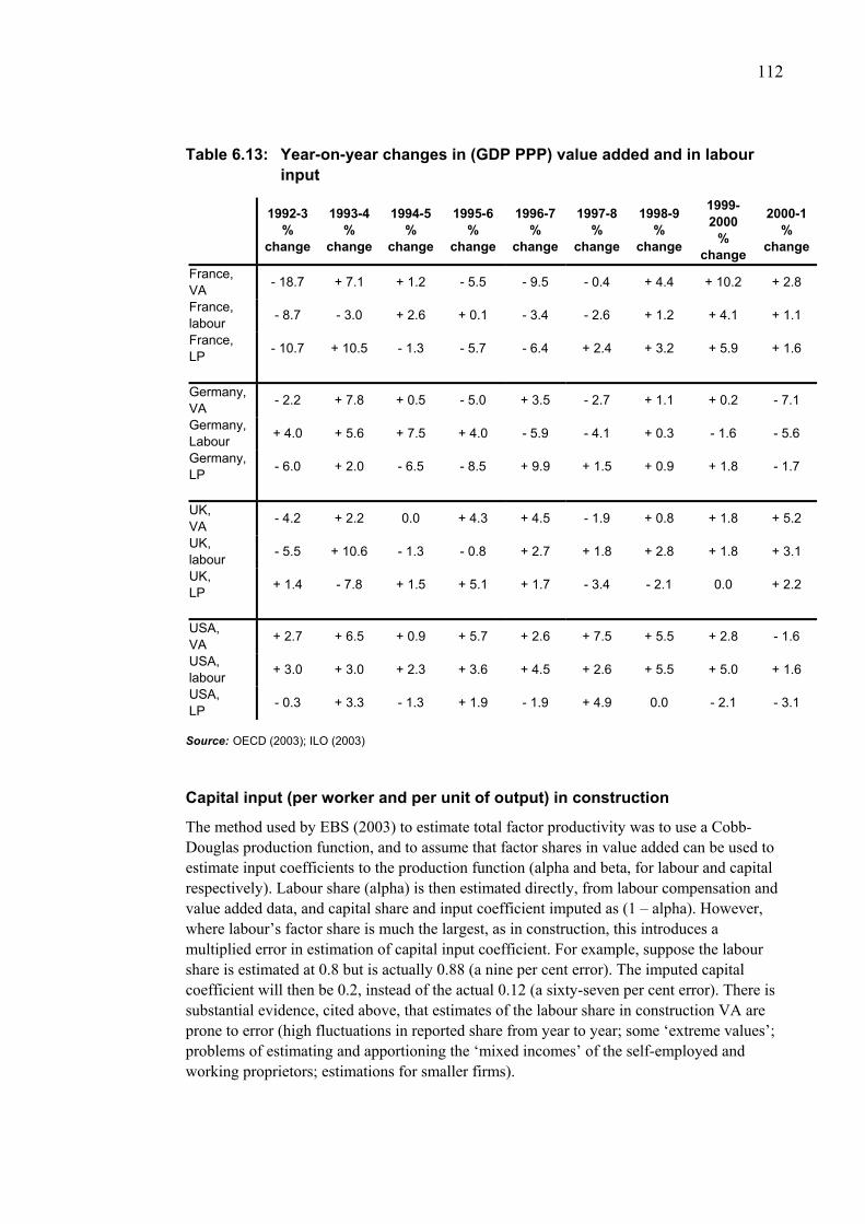
112

Table 6.13: Year-on-year changes in (GDP PPP) value added and in labour input

1992-3

% change

1993-4 %

change

1994-5 %

change

1995-6 %

change

1996-7 %

change

1997-8 %

change

1998-9 %

change

1999-2000

% change

2000-1 %

change

France, VA - 18.7 + 7.1 + 1.2 - 5.5 - 9.5 - 0.4 + 4.4 + 10.2 + 2.8

France, labour - 8.7 - 3.0 + 2.6 + 0.1 - 3.4 - 2.6 + 1.2 + 4.1 + 1.1

France, LP - 10.7 + 10.5 - 1.3 - 5.7 - 6.4 + 2.4 + 3.2 + 5.9 + 1.6

Germany, VA - 2.2 + 7.8 + 0.5 - 5.0 + 3.5 - 2.7 + 1.1 + 0.2 - 7.1

Germany, Labour + 4.0 + 5.6 + 7.5 + 4.0 - 5.9 - 4.1 + 0.3 - 1.6 - 5.6

Germany, LP - 6.0 + 2.0 - 6.5 - 8.5 + 9.9 + 1.5 + 0.9 + 1.8 - 1.7

UK, VA - 4.2 + 2.2 0.0 + 4.3 + 4.5 - 1.9 + 0.8 + 1.8 + 5.2

UK, labour - 5.5 + 10.6 - 1.3 - 0.8 + 2.7 + 1.8 + 2.8 + 1.8 + 3.1

UK, LP + 1.4 - 7.8 + 1.5 + 5.1 + 1.7 - 3.4 - 2.1 0.0 + 2.2

USA, VA + 2.7 + 6.5 + 0.9 + 5.7 + 2.6 + 7.5 + 5.5 + 2.8 - 1.6

USA, labour + 3.0 + 3.0 + 2.3 + 3.6 + 4.5 + 2.6 + 5.5 + 5.0 + 1.6

USA, LP - 0.3 + 3.3 - 1.3 + 1.9 - 1.9 + 4.9 0.0 - 2.1 - 3.1

Source: OECD (2003); ILO (2003)

Capital input (per worker and per unit of output) in construction

The method used by EBS (2003) to estimate total factor productivity was to use a Cobb-Douglas production function, and to assume that factor shares in value added can be used to estimate input coefficients to the production function (alpha and beta, for labour and capital respectively). Labour share (alpha) is then estimated directly, from labour compensation and value added data, and capital share and input coefficient imputed as (1 – alpha). However, where labour’s factor share is much the largest, as in construction, this introduces a multiplied error in estimation of capital input coefficient. For example, suppose the labour share is estimated at 0.8 but is actually 0.88 (a nine per cent error). The imputed capital coefficient will then be 0.2, instead of the actual 0.12 (a sixty-seven per cent error). There is substantial evidence, cited above, that estimates of the labour share in construction VA are prone to error (high fluctuations in reported share from year to year; some ‘extreme values’; problems of estimating and apportioning the ‘mixed incomes’ of the self-employed and working proprietors; estimations for smaller firms).

113

The method used by O’Mahony (1999) to estimate capital input was a compromise between simply summing net (i.e. after capital consumption or allowance for loss-of-efficiency of aging assets) capital stocks (as defined in National Accounting) and what O’Mahony (p41) calls the ‘ideal’ method – of using “the ideal user cost formula as outlined in Jorgenson et al (1987), employing the nominal internal rate of return plus nominal capital gains”. The standard formula for annual value of capital input equals the net stocks of assets multiplied by their user cost of capital, where the latter is given by the real interest rate plus depreciation minus real capital gains. This method requires prior knowledge of net stocks, which in turn requires knowledge of asset lives, as well as retirement patterns and the shape and value of relative-efficiency functions over time. Information on actual asset service lives is scarce, and the choice of form chosen for the loss-of-efficiency function is largely a matter of assumption.

Accordingly, we have tried to follow an alternative method for estimating capital input. This is based on decomposing the value of capital services per period into a ‘capital consumption’ and a ‘return on capital’ component; estimating the former; and assuming the latter is similar in each national industry under study. If we can estimate ‘capital consumption’ as a flow of value added, rather than as a proportion of an (unknown) capital stock, then we can work backwards to estimate the capital stock implied by a given value of capital consumption. We have simply assumed that, on average, capital consumption is just offset by gross capital expenditure, thus maintaining a constant capital stock. We follow Jorgenson et al, but assume that the only capital ‘gains’ are negative, i.e. depreciation. These assumptions yield a series of ‘pairs’ of possible values for average capital asset lives and for rates of return on capital, in each national industry, that are consistent with any given capital input coefficient in the production function. These can then be judged in terms of plausibility.

We have produced estimates, not of average physical capital stocks per employee, but of capital consumption per employee per year. In principle, this should be proportionate to the average relative ‘user cost’ value of capital services per employee in the construction industries of the three countries for which data was available.

Clearly, it is only relative values across countries that can meaningfully be compared using this method, which may yield estimates proportionate to, but not an absolute or cardinal measure of, the value of fixed capital services per period.

[This method is an alternative to the theoretical option of taking data for 45.1 to 45.4 only (i.e. excluding 45.5, plant-hire with operators) for gross capital expenditure plus data on payments by them to plant-hire firms. The Eurostat NewCronos database does not in fact contain data on payments for plant hire for France, but only for UK and Germany, thus limiting the value of this option.]

Our source is the Eurostat NewCronos database, which has disaggregated data on total gross capital expenditure and gross capital expenditure on machinery & equipment. Again data availability has restricted the analysis to three years, 1999-2001. Ideally we would have preferred to have data for the whole of a business cycle. Eventually, as new years’ data is added into the NewCronos database, this should become possible. The analysis includes the three European industries but we have been unable to find this sort of disaggregated data for the USA.

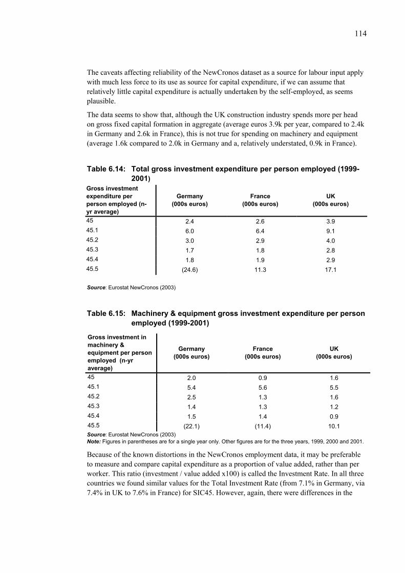
114

The caveats affecting reliability of the NewCronos dataset as a source for labour input apply with much less force to its use as source for capital expenditure, if we can assume that relatively little capital expenditure is actually undertaken by the self-employed, as seems plausible.

The data seems to show that, although the UK construction industry spends more per head on gross fixed capital formation in aggregate (average euros 3.9k per year, compared to 2.4k in Germany and 2.6k in France), this is not true for spending on machinery and equipment (average 1.6k compared to 2.0k in Germany and a, relatively understated, 0.9k in France).

Table 6.14: Total gross investment expenditure per person employed (1999-2001)

Gross investment expenditure per person employed (n-yr average)

Germany (000s euros)

France (000s euros)

UK (000s euros)

45 2.4 2.6 3.9 45.1 6.0 6.4 9.1 45.2 3.0 2.9 4.0 45.3 1.7 1.8 2.8 45.4 1.8 1.9 2.9 45.5 (24.6) 11.3 17.1

Source: Eurostat NewCronos (2003)

Table 6.15: Machinery & equipment gross investment expenditure per person employed (1999-2001)

Gross investment in machinery & equipment per person employed (n-yr average)

Germany (000s euros)

France (000s euros)

UK (000s euros)

45 2.0 0.9 1.6 45.1 5.4 5.6 5.5 45.2 2.5 1.3 1.6 45.3 1.4 1.3 1.2 45.4 1.5 1.4 0.9 45.5 (22.1) (11.4) 10.1 Source: Eurostat NewCronos (2003) Note: Figures in parentheses are for a single year only. Other figures are for the three years, 1999, 2000 and 2001.

Because of the known distortions in the NewCronos employment data, it may be preferable to measure and compare capital expenditure as a proportion of value added, rather than per worker. This ratio (investment / value added x100) is called the Investment Rate. In all three countries we found similar values for the Total Investment Rate (from 7.1% in Germany, via 7.4% in UK to 7.6% in France) for SIC45. However, again, there were differences in the

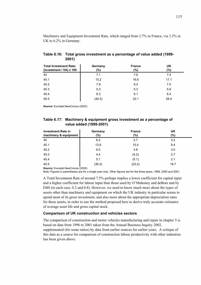
115

Machinery and Equipment Investment Rate, which ranged from 2.7% in France, via 3.2% in UK to 6.2% in Germany.

Table 6.16: Total gross investment as a percentage of value added (1999-2001)

Total Investment Rate: (investment / VA) x 100

Germany (%)

France (%)

UK (%)

45 7.1 7.6 7.4 45.1 15.2 16.6 17.1 45.2 7.9 8.4 7.5 45.3 5.3 5.3 5.9 45.4 6.3 6.1 6.4 45.5 (40.3) 22.1 28.4

Source: Eurostat NewCronos (2003)

Table 6.17: Machinery & equipment gross investment as a percentage of value added (1999-2001)

Investment Rate in machinery & equipment

Germany (%)

France (%)

UK (%)

45 6.2 2.7 3.2 45.1 13.9 15.4 9.4 45.2 6.5 3.8 3.0 45.3 4.4 (4.2) 2.7 45.4 5.1 (5.1) 2.1 45.5 (36.2) (23.2) 18.7 Source: Eurostat NewCronos (2003) Note: Figures in parentheses are for a single year only. Other figures are for the three years, 1999, 2000 and 2001.

A Total Investment Rate of around 7.5% perhaps implies a lower coefficient for capital input and a higher coefficient for labour input than those used by O’Mahoney and deBoer and by EBS (in each case, 0.2 and 0.8). However, we need to know much more about the types of assets other than machinery and equipment on which the UK industry in particular seems to spend most of its gross investment, and also more about the appropriate depreciation rates for these assets, in order to use the method proposed here to derive truly accurate estimates of average asset life and gross capital stock.

Comparison of UK construction and vehicles sectors

The comparison of construction and motor vehicles manufacturing and repair in chapter 5 is based on data from 1996 to 2001 taken from the Annual Business Inquiry 2002, supplemented (for some ratios) by data from earlier sources for earlier years. A critique of this data as a source for comparison of construction labour productivity with other industries has been given above.

116

In the case of the vehicles sector, however, our generally preferred source for labour input (LFS) is not available. Thus, if any comparison is to be made, it must perforce use ABI data. Chapter 5 examines the implications of the published material, used without adjustment.

The effect of the measurement problems associated with self-employment is that the ABI seriously overstates actual UK construction labour productivity. This must be borne in mind by the reader throughout chapter 5, especially where it deals with apparent relative levels of productivity between construction and vehicles industries, and thus in interpreting the findings summarised below.

An approximate quantification of this effect can be obtained by comparing UCL / DLC preferred estimate of construction LP in 1999, at current prices = £21,200

ABI-based estimate of construction LP in 1999 at current prices = £29,300 Thus the ABI-based estimate for construction LP is 38% higher than the UCL / DLC estimate

We recognise, however, than our LFS-based method for measuring construction labour, whilst the best method for international comparisons with other construction industries, is not ideal for comparisons with other UK industries for which no LFS-based estimates of labour input are available.

The ABI-based estimate of MVPR (motor vehicles production and repair) LP in 1999 at constant 1995 prices is £27,300, a weighted average of

£31,000 LP in SIC 34 (vehicles production) £22,000 LP in SIC 50.2 (vehicle repair and servicing)

The ABI-based estimate of all construction LP in 1999 at constant 1995 prices is £25,700.

The UCL / DLC estimate of construction LP in 1999 at constant 1995 prices is £18,100.

Adjusting MVPR labour upward by 18% (to allow for the fact that LFS reports a 18% larger figure for numbers employed across the whole economy than does ABI) gives adjusted LP for MVPR in 1999 at constant 1995 prices of £23,100. This is some 27% higher than our estimate for LP in 1999 in construction (£18,100) in constant 1995 prices.

The most striking findings from the comparison, undertaken using ABI data, would appear to be:

1. that the much higher levels of capital per worker found in SIC 34 (motor vehicles manufacture) compared to SIC 45 (all construction), yield it only a relatively modest labour productivity advantage over all construction.

2. that in each sector (motor vehicles and construction) much higher levels of labour productivity are found in new production than in repair activity

3. that construction R&M activity may have higher, or at least comparable, productivity than vehicles R&M activity.

4. that some major branches of new construction activity may have at least comparable productivity to vehicles production activity.

117

5. that the estimated relative labour productivity of the vehicles sector as a whole (production and repair) compared to construction as a whole depends heavily upon the weights used for production and repair; and it seems clear that the weight used for repair (by taking 50.2 only to stand for all repair and servicing activity) is too low, understating the relative size of the lower-productivity vehicle repair sub-sector.

6. that the rate of change in labour productivity per person in recent years (1998-2001) has probably been better in construction than in motor vehicles production; this differential remains even when one compares ABI-based data for output and labour, and thus for productivity change, in vehicles production with our preferred method (National Accounts data for output and LFS data for labour) for construction

• this shows LP falling in motor vehicles production by 4% p.a., and constant LP in construction

We undertook our investigation to compare productivities in construction and MVPR in parallel with our investigation into the alternative methods available for measuring construction LP.

In the light of the findings of the latter, it is now clear with hindsight that it would be desirable for the analysis on which the above findings are based to be re-done, using corrected and adjusted data for value added and labour input for all three industries (SICs 45, 34 and 50.2). Most especially, these corrections and adjustments should:

adjust numbers employed to include the self-employed and working proprietors

convert all labour input into total hours use the best available data for value added for each industry (for 45 this certainly means National Accounts value added)

Summing-up

Our headline finding suggests that the LP level of the UK construction industry is relatively poor compared to the three other countries studied, especially the USA and France. This is in partial contrast to other recent studies (O’Mahony and de Boer, 2002; Experian, 2003).

In addition, we find similar (negligible) rates of labour productivity growth in all four countries, for the period 1992 to 2001.

However, our analysis of various sectoral and sub-sectoral measures (data from Eurostat) suggests that the relative investment performance of the UK construction industry is surprisingly good in aggregate, but poor in terms of investment in machinery and equipment only.

Finally, definitive findings, even as to national rank orders in terms of productivity levels, are simply not possible at this stage, in the present state of the data. The table below indicates the main sources of error and the likely direction of the result of the correction of that error in the relative rankings and ratios of the four countries’ estimated construction productivities.

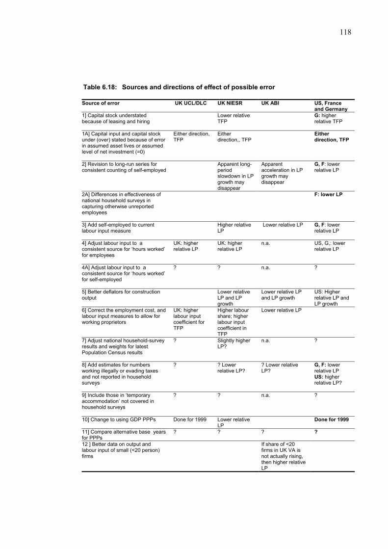
118

Table 6.18: Sources and directions of effect of possible error

Source of error UK UCL/DLC UK NIESR UK ABI US, France and Germany

1] Capital stock understated because of leasing and hiring

Lower relative TFP

G: higher relative TFP

1A] Capital input and capital stock under (over) stated because of error in assumed asset lives or assumed level of net investment (=0)

Either direction, TFP

Either direction,, TFP

Either direction, TFP

2] Revision to long-run series for consistent counting of self-employed

Apparent long-period slowdown in LP growth may disappear

Apparent acceleration in LP growth may disappear

G, F: lower relative LP

2A] Differences in effectiveness of national household surveys in capturing otherwise unreported employees

F: lower LP

3] Add self-employed to current labour input measure

Higher relative LP

Lower relative LP G, F: lower relative LP

4] Adjust labour input to a consistent source for ‘hours worked’ for employees

UK: higher relative LP

UK: higher relative LP

n.a. US, G,: lower relative LP

4A] Adjust labour input to a consistent source for ‘hours worked’ for self-employed

? ? n.a. ?

5] Better deflators for construction output

Lower relative LP and LP growth

Lower relative LP and LP growth

US: Higher relative LP and LP growth

6] Correct the employment cost, and labour input measures to allow for working proprietors

UK: higher labour input coefficient for TFP

Higher labour share; higher labour input coefficient in TFP

Lower relative LP

7] Adjust national household-survey results and weights for latest Population Census results

? Slightly higher LP?

n.a. ?

8] Add estimates for numbers working illegally or evading taxes and not reported in household surveys

? ? Lower relative LP?

? Lower relative LP?

G, F: lower relative LP US: higher relative LP?

9] Include those in ‘temporary accommodation’ not covered in household surveys

? ? n.a. ?

10] Change to using GDP PPPs Done for 1999 Lower relative LP

Done for 1999

11] Compare alternative base years for PPPs

? ? ? ?

12 ] Better data on output and labour input of small (<20 person) firms

If share of <20 firms in UK VA is not actually rising, then higher relative LP

119

13 ] Revise (add to) estimated unrecorded output incorporated in National Accounts

? ? n.a. ?

14 ] Convert US value added to basic prices, to remove sales taxes levied on construction output

US: lower relative LP and TFP

15] Use alternative years for comparison of levels of LP

? ? ? ?

120

7 Conclusions, principal findings and recommendations

This report gives a picture of productivity in the construction industry from available data. There are two types of flaws in the data. The first concerns data gathering techniques which are the professional concern of statisticians. The main weaknesses in the data concern the definition of industrial classifications within the construction industry in SIC and NACE, missing data and the problems of international comparability.

The second concerns the differences between the quantitative information supplied and a qualitative account of the construction industry based on a variety of sources such as academic papers and the experience of those engaged in the industry. The picture of productivity in the UK construction industry that emerges from the data and statistics we have been able to obtain and analyse is that UK construction industry performance appears to be very different from that in the USA.

This picture however, has to be qualified, qualitative differences in the output both in terms of finishes and in terms of different building types are not fully captured by the data. Perhaps they never could be.

Conclusions and recommendations

1. The best available dataset for international comparison of construction productivity levels or for study of trends is that of the NIESR. This is superior in several ways to ABI / CoP-derived international datasets, principally that held by Eurostat.

2. However, further work is required to improve the construction element of the NIESR dataset

• On PPPs

• On deflators (outside UK)

• On self-employment (outside UK)

3. Research is required comparing each country’s LFS results for employees (as well as self-employed) in construction with that country’s employer-based survey results for employees.

4. It would be highly desirable to add questions eliciting value added to the DTI’s PCC survey of construction firms.

5. An investigation is needed definitively to determine what has been happening to the methods and assumptions underlying the UK CoP / ABI data for construction since 1995.

6. Research is needed on developing a feasible but reasonably accurate method for measuring the value of capital inputs in each country’s construction industry, but especially in the UK.

121

Findings

1. For construction, the reported ‘productivity gaps’ for levels between the UK and the US, France and Germany appear quite large but may be within the margins of error of the data used.

2. Further work removing sources of error might either widen or narrow these reported gaps.

3. Definitive findings, even as to national rank orders in terms of productivity levels, are simply not possible at this stage, in the present state of the data.

4. All that we can do here is to indicate the main sources of error and the likely direction of the result of correction of that error in the relative rankings and ratios of the four countries’ estimated construction productivities.

5. Recent rates of change in labour productivity, in all four countries, appear to be negligible.

6. Labour productivity in each ‘branch’ of construction (new construction and repair & maintenance) may be surprisingly close to labour productivity in the equivalent branch (motor vehicle production and motor vehicle servicing and repair) of the vehicles industries.

7. The UK construction industry has surprisingly high labour productivity, given its apparently much lower levels of capital per worker, compared with either:

a) the construction industries of other countries (especially, Germany) b) the motor vehicles production and repair industries in the UK

122

References

Allmon E, Haas C, Borcherding J and Goodrum P (2000) ‘US construction labour productivity trends, 1970-1998’, Journal of Construction Engineering and Management, March / April, 126, 97-104

Bon, R & Crosthwaite, D (2000) The Future of International Construction, Thomas Telford, London.

DTI (2002) Annual Construction Statistics, www.dti.gov.uk/statistics/constat2002

Daffin C (2001) ‘Introducing new and improved labour productivity data’, Economic Trends, No. 570, May

Daffin C and E Lau (2002) ‘Labour productivity measures from the Annual Business Inquiry’, Economic Trends, No. 589, December

Dodge (1998) Dodge cost guides, New York, McGraw Hill

Drew C, C Richardson and P Vaze (2001) ‘International comparisons of productivity – an update on developments’, Economic Trends, No. 570, May

EBS (2003) Sector Competitiveness Analysis for the Construction Industry, Experian Business Strategies, Draft.

Eisner R (1994) The misunderstood economy, Boston, Harvard Business School Press

Euroconstruct (1997) European Construction Trends 1996, CFR.

Euroconstruct (1999) European Construction Trends 1998, CFR.

Eurostat (2002) European Business Facts and Figures 1999 – 2000

Eurostat Working Paper (1998) Documentation of Eurostat’s database on international migration: labour data, WP 3 / 1998 /E / no. 16

Eurostat (2003) Structural Business Statistics Database, www.europa.eu.int/newcronos

Goodrum P, Haas C and Glover R (2002) ‘The divergence in aggregate and activity estimates of US construction productivity’, Construction Management and Economics, 20. 415-423

Goodrum P and Haas C (2002) ‘Partial factor productivity and equipment technology change at activity level in US construction industry’, Journal of Construction Engineering and Management, Nov / Dec, 128, 463-472

Goodrum P and Haas C (2001) ‘US construction productivity trends, 1970-1998: closure’, Journal of Construction Engineering and Management, Sept / Oct, 127, 428-429

Griliches Z (1988) ‘Productivity puzzles and R&D: another non-explanation’, Journal of Economic Perspectives, 2 (4), 9-21

Gruneberg S and G Ive (2000) Economics of the modern construction firm, Basingstoke, Macmillan

123

Gullickson W and Harper M (1999) ‘Possible measurement bias in aggregate productivity growth’, Monthly Labour Review, February, 47-67

Harley E and J Jones (1998) ‘International comparisons of productivity and wages’, Economic Trends, No. 530, January

ILO (2003) Labour Statistics, www.laborsta.ilo.org

Ive G and S Gruneberg (2000) Economics of the modern construction sector, Basingstoke, Macmillan

Linder M (1999) Wars of attrition, Iowa City, Fanpihua Press

Meager N (1992) ‘Self-employment in the European Community’, Paper presented at conference on Labour market institutions in Europe, Wissenschaftszentrum fur Sozialforschung, Berlin, December

Means Company (1998) Building construction cost data, Kingston Mass., Means Company Inc.

NIESR (2002) Sectoral Productivity Dataset, www.niesr.ac.uk/research/nisec

NIESR (1999) The National Institute Sectoral Productivity Database; Sources and Methods, www.niesr.ac.uk/research/nisec

OECD (2003) Annual National Accounts, www.oecd.org

ONS (2002) Annual Business Inquiry, London, The Stationery Office.

ONS (2002a) Motor Vehicle Production Inquiry, May 2002, BM PM 34.10

ONS (1996) Car and Commercial Vehicle Production, Oct 1996

ONS (2000) UK National Accounts: the Blue Book, London, The Stationery Office

ONS (1996) SDA 27 Results of the 1994 Motor Trades Survey

Sector Review Motor Trades (formerly SDA 27) for subsequent data

ONS (1998) Report on the Census of Production: summary volume, The Stationery Office, London.

ONS (1992) Report on the Census of Production: summary volume, The Stationery Office, London.

ONS (1988) Report on the Census of Production: summary volume, The Stationery Office, London.

O’Mahony M (1999) Britain’s productivity performance 1950-1996: an international perspective, London, NIESR

O’Mahony M. and deBoer W (2002) Britain’s relative productivity performance: updates to 1999. Final Report to DTI/Treasury/ONS

O’Mahony M and deBoer W (2002A) ‘Britain’s relative productivity performance: has anything changed?’ National Institute Economic Review, 179, 38-43

Oppedahl D (2000) ‘Understanding the (relative) rise and fall of construction real wages’, Chicago Fed. Letter, 155, July, 1-4

124

Pieper P (1990) ‘Measurement of construction prices: retrospect and prospect’ in Berndt E and Triplet J (eds.) Fifty years of economic measurement, Chicago, U of Chicago Press

Pieper P (1989) ‘Construction price statistics revisited’ in Jorgenson D and Landau R (eds.) Technology and capital formation, Cambridge, Mass., MIT Press

Pilat D (2002) ‘International comparisons of productivity – key findings and measurement issues’, OECD

Rees A (1980) ‘Improving productivity measurement’, American Economic Review, 70

Richardson C (2001) ‘International comparisons of productivity’, Economic Trends

Teicholz P (2001) ‘US construction labour productivity trends, 1970-98: discussion’, J of Construction Engineering and Management, Sept / Oct, 127, 427-428

Teicholz P (2000) ‘Productivity trends in the construction industry’, Proc. 2000 American Institute of Steel Construction Annual Convention, Chicago

US Bureau of Labor Statistics: http://stats.bls.gov

US Bureau of Labor Statistics (1997) Handbook of methods, Bulletin 2497

US Department of Commerce (2000) Census of Construction Industries 1997, Washington DC, Bureau of the Census.

US Department of Commerce (1998) Value of construction put in place, Construction Report Series C30, Bureau of the Census

US Department of Commerce (1995) Census of Construction Industries 1992, Washington DC, Bureau of the Census.

Whisler, T.R. (1999) The British Motor Industry 1945-1994, Oxford, OUP

World Bank (2001) World Development Indicators 2001

http://europa.eu.int/comm/eurostat/structuralindicators

http://qb.soc.surrey.ac.uk/surveys/lfs

www.statistics.gov.uk

www.data-archive.ac.uk

Appendices

Appendix A

Terms of reference

With reference to an email letter dated 15th November 2002 from Mr Chris Nicholls to Mr Graham Ive, the authors have been asked to produce a report (a) on levels of productivity and (b) on trends in annual changes in productivity (c) on estimates of capital stock per employee in construction in different countries, and (d) on a comparison between the UK’s construction industry’s new and repair and maintenance sectors with those of automotive manufacturing and repair and maintenance. In particular the report will show:

a) Estimates of average labour productivity levels in different sectors of construction in the UK, France, Germany and the USA.

b) Estimates of recent trends in annual growth rates of labour productivity in different sectors of construction in the UK, France, Germany and the USA.

c) Estimates of average physical capital stocks per employee (or employee-hour) in the different sectors of construction in the UK, France, Germany and the USA.

d) Estimates of average labour productivity levels in different sectors of construction in the UK compared with average labour productivity levels in comparable branches of the UK automotive industries (e.g. auto manufacturing, vehicle repair and maintenance).

e) Description of methodologies used for each section.

Appendix B

Sources and Methodology

General comments on the statistical sources.

We have based our report on data from Annual Construction Statistics (DTI), Eurostat, the Office of National Statistics and the NIESR. Unfortunately we found many of the tables we wished to use contained missing data. We also found discrepancies in the data on employment when we compared different sources. For this reason we have in the main followed advice from the NIESR that ONS employment data estimates of construction employment were more reliable than the data found in the Annual Construction Statistics. Although we would have liked to calculate capital stocks from data found in PRODCOM, we found the data to contain missing information, which we could not meaningfully estimate in the time available.

Levels of productivity

We use:

• All-construction (NACE 45) and NACE 451 to 455 value-added per annum at current prices

• All-construction (NACE 45) and NACE 451 to 455 labour input per annum

• The All New Construction Index to deflate all-construction (NACE 45) and NACE 451 to 455 value-added to constant prices and the implied GPD deflator to deflate the motor industry data (NACE 34).

• Derived or implied estimates of all-construction (NACE 45) and NACE 451 to 455 labour productivity (value-added in national currency units at constant prices per time unit of labour input).

Although the Eurostat data appears at first glance to offer the following information, many tables were incomplete to the extent that useful analysis and international comparisons of levels and trends were not practical in the time available.

The tables found contained the following variables:

Firms by employment size: 1- 9, 10 - 19, 20+, Total and 1 - 19.

Number of enterprises

VA at basic prices

VA at factor cost

Wages and salaries

Number employed

Number of unpaid persons employed

Number of employees

Gross VA per person (apparent labour productivity)

Gross VA per unit personnel cost (simple adjusted labour productivity)

Gross VA per employee

Gross VA per hour worked by employees

Labour cost per employee (unit labour cost)

VA at factor cost in production value

Turnover or gross premiums written

Production value

Turnover per person employed

Comments on the Eurostat data

The vast majority of tables give UK and French data for 1996-2000 but only 1999-2000 for Germany. Value-added at basic prices are only available for UK. Some UK series have no data for 1998 and some UK data for 2000 is given as provisional.

The best data sets are for size of firms in the 20+ class, where data for UK and France is from 1995-2000 and Germany 1996-2000, but even in this size group turnover per person employed is for UK and France only. Value added at basic prices is given for UK only but value added at factor cost is good for all 3 countries.

While it had been hoped to carry out an international comparison of annual changes in productivity by size of firm, this data was not readily available. In principle the data sets should have been published by Eurostat, but the information was found to be missing.

UK CI and vehicles manufacturing and R and M

Comparative data from the ONS based on the Annual Business Inquiry was used. Our main data source for the automotive industry is the Business Monitor 34.10, Motor Vehicle and Engine Production Inquiry (MVEPI) for physical output of cars.

For vehicle dealing and R and M, the Motor Trades Inquiry Annual Business Monitor SDA 27 contains turnover, stocks, employment costs, purchases, capital expenditure based on a stratified random sample of smaller firms. The SDQ 11 covers all services including motor trades.

We used the Annual Business Inquiry for the comparison of real output with the construction industry. The respective SIC’s are described below.

SIC 92 34 Manufacture of motor vehicles, trailers and semi-trailers

This class includes:

o Manufacture of passenger cars

o Manufacture of commercial vehicles:

Vans, lorries, over-the-road tractors for semi-trailers, dumpers for off road use, etc

o Manufacture of bodies for motor vehicles

o Manufacture of parts and accessories for motor vehicles

o Manufacture of buses, trolley-buses and coaches

o Manufacture of motor vehicle engines

o Manufacture of chassis fitted with engines

o Manufacture of other motor vehicles:

Snow mobiles, golf carts, amphibious vehicles, fire engines, street sweepers, travelling libraries and banks, etc

This class excludes:

Manufacture of agricultural and industrial tractors

Manufacture of electrical parts for motor vehicles

Maintenance, repair and alteration of motor vehicles

SIC 92 50.20 Maintenance and repair of motor vehicles

This class includes:

o Maintenance and repair of motor vehicles:

Mechanical repairs

Electrical repairs

Ordinary servicing

Bodywork repair

Repair of motor vehicle parts

Washing and polishing, etc

Spraying and painting

Repair of screens and windows

o Tyre and tube repair, fitting and replacement

o Anti-rust treatment

o Installation of parts and accessories

o Roadside assistance

This class excludes:

Retreading and rebuilding tyres

Maintenance and repair of caravans

Productivity and labour costs based on European Business Facts and Figures, Eurostat

It should be noted that the data set is incomplete and that ratios for several countries in several years are not available. However, using available data from Eurostat (European Business Facts and Figures 1999 – 2000, Eurostat) we have attempted a summary of international comparison of productivity ratios.

According to Eurostat approximately 6 million persons or 56% of total employment in the European construction industry could be accounted for under site preparation and construction activities in 2000, (European Business Facts and Figures 1999 – 2000, Eurostat, p. 288). The share of site preparation and construction activities in total construction VA was greater than in the other sub-sectors of construction, implying higher productivity.

Between 1992 and 2000 the wage-adjusted labour productivity ratio for NACE Groups 45.1 and 45.2 (site preparation and general construction) in most EU countries was generally above 110%. In 1999 it was above 120%. In 1997 the UK ratio had been 157.9%. The only countries, which dropped below 110% were France and the Netherlands in 1998 with 107.8% and 105.6% respectively. According to Eurostat, these figures may be explained by the relatively high labour costs in France and the Netherlands compared to the UK, though this contradicts the evidence given in Figure 2.18 in this report. While the average personnel costs per employee in site preparation and general construction in the EU was €35,300 in 1998, in the UK the equivalent cost per employee was only €31,800 in 1997. The lowest costs were in Portugal at €11,200.

Employment in the NACE Groups 45.3 and 45.4 (installation and completion) was estimated to be just under 5 million persons. This sub-division of the construction industry includes

• installation of electrical wiring and fittings

• insulation

• plumbing

• plastering

• joinery installation

• floor and wall covering

• painting and glazing, and

• other building and installation and completion activities

In 1999 the wage adjusted labour productivity ratio of this sub-division, taken as a whole, was less than 115%. According to Eurostat (European Business Facts and Figures 1999 – 2000, Eurostat, p.290), the lowest ratios occurred in Belgium at 101.8% and France at 105.8%, while the highest ratios were found in Finland at 127.7% and in the UK (in 1997)

with 141.7%. These differences arise from disparities in apparent labour productivity because Belgium, France, Finland and the UK all had very similar average personnel costs per employee in the installation and completion sub-sectors of between €28,500 in Finland and €30,300 in the UK.

In other words while differences in productivity in site preparation and general construction may be attributed to differences in employment costs, in installation and completion the differences may be accounted for by differences in apparent labour productivity.

Annual rates of change

To calculate average annual rates of change we have used the coefficient of the log regression, namely:

y = mlnx + c.

Comments on NIESR (2002) sources and methodology

Sector and data coverage

The NIESR (2002) dataset provides annual data for the post war period from 1950 to 1999 for five major industrial economies, the United States, the United Kingdom, France, Germany and Japan. The variables included in the dataset are real output, persons engaged, annual average hours worked, labour productivity, capital input, labour force skills and labour’s share of value added. Ten broad sectors are covered including the construction sector.

Industry classifications

The NIESR attempted as far as possible to match the industry classifications in the five countries. The starting point was taken to be the UK Standard Industrial Classification, 1992 version (SIC 92) and other countries classification systems were adjusted to render them as close as possible to the British system.

Output

Output data are presented in index form with 1996 set equal to 100. For each sector data were taken from the national accounts and generally are equal to gross value added at constant prices.

Persons engaged

Persons engaged includes all full-time and part-time employees and self-employed persons. In general standard sources include the self-employed but for the UK published sources by sector generally only include employees in employment. Therefore some additional estimation was required for the UK.

‘Official time series do not exist for the self-employed by sector in the UK’ (NIESR, 1999). The NIESR therefore resorted to the population census to estimate the proportion of self-employed in total persons engaged. Linear interpolation was used to estimate these proportions between census years. Adjustments to include self-employed had large impacts in various sectors but particularly in the construction sector.

Annual average hours worked

Average annual hours worked per employee were constructed for each of the five countries from a variety of sources. These series are less reliable and involve more non-comparabilities than number of persons engaged. Average annual hours worked is the product of two components, average weekly hours and average weeks worked per year. For reasons of international comparability hours worked are primarily based on firm level data (establishment surveys) on weekly hours combined with weeks worked per year.

The estimation of capital stocks

Investment data was largely taken from unpublished government sources. Net capital stocks were employed in the NIESR dataset calculated separately for equipment and structures. Published depreciation rates were used. These rates were available by asset type and were converted to sector specific depreciation rates for equipment and structures. In construction these were 0.161 for equipment and 0.0286 for structures.

In calculating relative levels of capital input, purchasing power parities were used to convert investment in domestic currencies to US $. The equipment PPPs were sector specific estimates, derived as weighted averages of PPPs for three asset types, machinery, vehicles and computers, with weights equal to each sector’s share of US investment in these assets. Leased assets were allocated where feasible to the sector of use rather than sector of ownership.

Labour’s share of value added

This is calculated as labour compensation (this includes wages and salaries for employees and non-wage labour costs such as employer’s contributions to national insurance and pensions) plus the imputed labour of the self-employed divided by nominal gross domestic product. The inclusion of imputed compensation for the self-employed is important in the construction sector, failure to take account of the self-employed would place far too high a weight on capital in the total factor productivity calculations. The basic sources were national accounts totals supplemented where necessary by information from annual censuses.

The estimation of relative productivity levels

In constructing productivity levels the most difficult problem is how to measure output in a manner, which is comparable across countries. There are two methods to achieve this; either deflate bilateral ratios of nominal output in a sector by the ratios of a country’s output prices or base output on some quantity indicator.

The price ratios used to deflate nominal value added can be based on price quotations for specific products, unit value ratios (the ratio of values of sales divided by quantities produced) or purchasing power parities (the ratio of final expenditure prices estimated periodically by international bodies such as Eurostat or OECD).

In the NIESR data purchasing power parities for 1996 were used to convert nominal outputs to £ sterling. Price ratios were calculated using unpublished data, provided by Eurostat, giving PPPs and expenditures for about 150 individual categories. The sector PPPs were constructed by choosing the items which corresponded most closely to the outputs of the sector. The price ratios for construction were based on PPPs for buildings.

In constructing aggregate sector price ratios individual PPPs were weighted by expenditure shares using the EKS multilateral weighting system for the four countries. The latter ensures that pair-wise comparisons between countries are transitive. The EKS system generates transitive international comparisons that minimise deviations from direct binary comparisons.

The NIESR (2002) research estimates productivity per joint units of labour and capital, measured as total factor productivity, using the method of growth accounting.