arX

iv:q

-bio

/030

9027

v1 [

q-bi

o.N

C]

16 A

pr 1

998

Measuring the dynamics of neural responses in primary

auditory cortex

Didier A.Depireux, Jonathan Z. Simon and Shihab A.Shamma

Electrical Engineering Department & Institute for Systems ResearchUniversity of Maryland

College Park MD 20742–3311, USA(301) 405-6842

We review recent developments in the measurement of the dynamics of the response propertiesof auditory cortical neurons to broadband sounds, which is closely related to the perception oftimbre. The emphasis is on a method that characterizes the spectro-temporal properties ofsingle neurons to dynamic, broadband sounds, akin to the drifting gratings used in vision.The method treats the spectral and temporal aspects of the response on an equal footing.

Keywords: Auditory cortex, Spatial frequency, Temporal frequency, Separability, Ripples

Contents

1 Introduction 31.1 Timbre . . . . . . . . . . . . . . . . . . . . . . . . . . . . . . . . . . . . . . . . . 31.2 Auditory Cortex . . . . . . . . . . . . . . . . . . . . . . . . . . . . . . . . . . . 3

2

2 Background 42.1 Response Field . . . . . . . . . . . . . . . . . . . . . . . . . . . . . . . . . . . . 42.2 Natural Sounds . . . . . . . . . . . . . . . . . . . . . . . . . . . . . . . . . . . . 52.3 Auditory Pathway (Monaural) . . . . . . . . . . . . . . . . . . . . . . . . . . . . 6

3 Principles 63.1 Guiding Principles . . . . . . . . . . . . . . . . . . . . . . . . . . . . . . . . . . 73.2 Response Field and Linearity . . . . . . . . . . . . . . . . . . . . . . . . . . . . 73.3 Spectro-Temporal Response Field . . . . . . . . . . . . . . . . . . . . . . . . . . 83.4 Transfer Functions . . . . . . . . . . . . . . . . . . . . . . . . . . . . . . . . . . 83.5 Full Separability . . . . . . . . . . . . . . . . . . . . . . . . . . . . . . . . . . . . 93.6 Quadrant Separability . . . . . . . . . . . . . . . . . . . . . . . . . . . . . . . . 103.7 Confirming Separability . . . . . . . . . . . . . . . . . . . . . . . . . . . . . . . 103.8 Confirming Linearity . . . . . . . . . . . . . . . . . . . . . . . . . . . . . . . . . 103.9 Characterizing the Response . . . . . . . . . . . . . . . . . . . . . . . . . . . . . 10

3.9.1 Amplitude of the response . . . . . . . . . . . . . . . . . . . . . . . . . . 113.9.2 Phase of the response . . . . . . . . . . . . . . . . . . . . . . . . . . . . . 11

4 Analytical Methods 124.1 The Ripple Stimulus . . . . . . . . . . . . . . . . . . . . . . . . . . . . . . . . . 134.2 Data Analysis . . . . . . . . . . . . . . . . . . . . . . . . . . . . . . . . . . . . . 144.3 Separability . . . . . . . . . . . . . . . . . . . . . . . . . . . . . . . . . . . . . . 154.4 Linearity . . . . . . . . . . . . . . . . . . . . . . . . . . . . . . . . . . . . . . . . 16

5 Experiment and Results 175.1 Experimental Details . . . . . . . . . . . . . . . . . . . . . . . . . . . . . . . . . 175.2 Obtaining the Transfer Functions . . . . . . . . . . . . . . . . . . . . . . . . . . 17

5.2.1 Spectral cross-section of the transfer function . . . . . . . . . . . . . . . 175.2.2 Temporal Cross-Section of the Transfer Function . . . . . . . . . . . . . 18

5.3 Quadrant Separability . . . . . . . . . . . . . . . . . . . . . . . . . . . . . . . . 215.4 Quadrant Linearity . . . . . . . . . . . . . . . . . . . . . . . . . . . . . . . . . . 215.5 Full-Quadrant Separability and Linearity . . . . . . . . . . . . . . . . . . . . . . 225.6 Response Characteristics . . . . . . . . . . . . . . . . . . . . . . . . . . . . . . . 22

6 Conclusions 22

7 Acknowledgements 25

8 References 25

List of Figures

1 Location and tonotopy of Primary Auditory Cortex . . . . . . . . . . . . . . . . 42 Examples of idealized RFs . . . . . . . . . . . . . . . . . . . . . . . . . . . . . . 53 Spectral envelope of a vowel . . . . . . . . . . . . . . . . . . . . . . . . . . . . . 5

3

4 Spectro-temporal envelope of a ripple . . . . . . . . . . . . . . . . . . . . . . . . 85 The w-Ω plane . . . . . . . . . . . . . . . . . . . . . . . . . . . . . . . . . . . . 96 Characterizing the phase of the transfer function . . . . . . . . . . . . . . . . . . 127 Phase curves . . . . . . . . . . . . . . . . . . . . . . . . . . . . . . . . . . . . . . 128 Generating the ripple stimulus . . . . . . . . . . . . . . . . . . . . . . . . . . . . 139 Schematic of the response . . . . . . . . . . . . . . . . . . . . . . . . . . . . . . 1410 Computing the transfer function . . . . . . . . . . . . . . . . . . . . . . . . . . . 1511 Computing the transfer function: worst-case scenario . . . . . . . . . . . . . . . 1612 Computing the transfer function: actual scenario . . . . . . . . . . . . . . . . . 1613 Measuring a spectral cross-section of the transfer function . . . . . . . . . . . . 1914 Measuring a temporal cross-section of the transfer function . . . . . . . . . . . . 2015 Experimental measurement of one-quadrant separability . . . . . . . . . . . . . 2116 Experimental measurement of one-quadrant linearity . . . . . . . . . . . . . . . 2317 Experimental measurement of quadrant linearity . . . . . . . . . . . . . . . . . . 24

1 Introduction

1.1 Timbre

We classify everyday natural sounds by their loudness (related to the intensity of the sound),their pitch (the perceived tonal height) and their timbre (the quality of the sound; that which isneither loudness nor pitch). The perception of timbre, which will be the main focus of this paper,is what allows us to tell the difference between two vowels spoken with the same pitch, or thedifference between a clarinet and an oboe playing the same note. When hearing several musicalinstruments simultaneously, we can usually tell which instruments are playing by identifyingthe different timbres present in the mixed sound. Additionally, the perception of timbre isquite robust in the presence of noise and echoes (or reverberations), or even severe degradationsuch as during a telephone conversation, in which the sound is severely band-passed. Timbreperception is therefore an essential attribute of our sense of hearing.

To understand how we extract these different aspects of a sound, we must unravel whatthe auditory representation is along the neural pathway. The approach presented here takesthe point of view that the principles used by neural systems are universal, once the stimulushas reached beyond the sensory epithelium (whether the cochlea’s basilar membrane or theretina). In particular the ideas presented here are frequently guided by considering the basilarmembrane as a spatial axis, analogous to a one-dimensional retina, and then using the methodsof visual gratings (drifting and otherwise), to study and characterize cells in the auditory cortex.

1.2 Auditory Cortex

A few general organizational features have long been recognized in Primary Auditory Cortex(AI), the location of which is shown in Figure 1. First is a spatially ordered tonotopic axis,along which cell responses are tuned from low to high frequencies1; this is alternatively called acochleotopic axis, which reflects the activity along the cochlea. Note that there are many fields

4

High

Low

AAF

AI

Area ofmagnification

Rostral Caudal

High

Low

Figure 1: The position of the Primary Auditory Cortex (AI) in the ferret brain. The location of theAnterior Auditory Field (AAF) for illustration purposes. On the right the tonotopic axis is overlaidfor both AI and AAF.

in the auditory cortical area (the Anterior Auditory Field is shown in Figure 1), most of whichdisplay a tonotopic organization.

Second, perpendicular to the tonotopic axis, cells are arranged in alternating bands accord-ing to binaural properties: bands of cells are alternatively excited or inhibited by stimulation ofthe ipsilateral ear (the contralateral ear usually produces an excitatory response2). The tono-topic and binaural dominance organization is analogous to the retinotopic and ocular dominancecolumns of visual cortex. Other parameters have also been used to describe characteristics thatchange systematically along isofrequency lines. Using combinations of two pure tones, one canmeasure the Response Area (RA), also known as frequency-threshold curve, i.e. the responsethreshold of a cell as a function of the tone frequency presented. It has been shown that mostRAs are topographically organized along the isofrequency lines according to the symmetry oftheir excitatory and inhibitory sidebands3. Other parameters have been also been shown tochange systematically in cat, such as threshold4, bandwidth5 and frequency modulation direc-tion selectivity3,6.

These properties of AI cells are derived using pure tones (or clicks) akin to using dots oflight (or flashes) to study cells in the visual pathway. Below we explain how to use the auditoryversion of drifting gratings7 to characterize response properties of cells to dynamic broadbandsounds. This is necessary to gain insight to how timbre is encoded. Another advantage of themethod presented here is that it allows us to determine the temporal and spectral properties ofa cell at the same time. In particular, one can study whether and to what extent the responsefield varies as a function of time, thereby characterizing the cell with a full spectro-temporalresponse field.

2 Background

2.1 Response Field

Traditionally, cells along the auditory pathway have been characterized by their RA, or tuningcurve. Determined using pure tones and by modifying the frequency of the stimulus whileadjusting its intensity, the RA is the frequency-intensity combinations that elicit a thresholdresponse, whether the sustained activity level or the strength of the onset response. In this

5

0

+

–

Frequency (kHz) [Octaves].5 [0] 1 [1] 2 [2] 4 [3] 8 [4] 16 [5]

Excitatory

Inhibitory

RF

Str

engt

h

Figure 2: Two idealized RFs at a given time. One RF (unbroken line) is centered on low frequenciesand is asymmetric, and the other (broken line) is centered on high frequencies and is symmetric.

0 1 2 3 40

40

80

Frequency (Hz)

Am

plitu

de

Figure 3: The spectrum of /aa/ spoken by one of the authors, with the spectral envelope superim-posed on it.

paper, we use the Response Field (RF), a function measured using broadband sounds. Asillustrated in Figure 2, it roughly reflects the range of frequencies that influence the dischargeproperties of the neuron under study. It is given in the form of a function, with positivevalues describing excitation (proportional to the RF’s amplitude) and negative values describinginhibition. In general, the RF is a spectro-temporal function, as opposed to the RA whichtypically describes only static properties (but see Nelken8 et al and Sutter9 et al). The definitionof RF will be made more precise later.

2.2 Natural Sounds

Natural sounds, such as environmental sounds, music and speech, are classified along severalperceptual axes. We typically describe a sound by its loudness, its pitch and its timbre. Pitchis what changes when we pronounce the same vowel with different tonal heights, e.g. the pitchof a female voice is typically higher than the pitch of a male voice. Timbre is what changeswhen, keeping the same tonal height, we pronounce different vowels (e.g. /ah/, /eh/, /ih/).Figure 3 illustrates the spectral profile or envelope of a sound. The envelope of a sound can beviewed as a low-order polynomial fit of the (time-windowed) spectrum of the sound. A commonmethod for the extraction of the envelope is the Linear Predictive Method (LPC)10; we will notgo into the details of LPC here, instead referring the reader to the intuitive notion of envelopeillustrated in Figure 3.

The percept of timbre has been typically ascribed to the extraction of the envelope of thespectrum, but it also includes the temporal variations in the spectral envelope (for instance,

6

the sound of a piano note played backwards sounds more like that of a wind organ, eventhough the amplitude of the Fourier transform of a sound and its time-reversed version areidentical). Therefore, the study of how timbre is encoded must include temporal as well asspectral properties of the system. For speech, the temporal variations in timbre involve time-scales of about 10 Hz, so that this dimension of time is different from the temporal frequenciesthat make up sounds. It is the extraction of the dynamic spectral envelope by the auditorycortex that we are concerned with. Because we are interested in timbre, we use pitchless,dynamic, broadband sounds as stimuli.

2.3 Auditory Pathway (Monaural)

The auditory pathway up to primary auditory cortex, ignoring structures usually considereddedicated to binaural aspects of sounds (such as localization) can be minimally described asfollows. The vibrations of the tympanic membrane are mechanically transformed into a travelingwave in the cochlea, with a profile that depends on the frequency content of the acousticspectrum. The vibrations of the basilar membrane are transformed by inner hair cells intopatterns of neural activity in the auditory nerve. For practical purposes, we can think of thebasilar membrane as a collection of 1/3 octave filters, performing a time-windowed Fouriertransform, with a time characteristic of about 30 ms. The auditory nerve projects to theCochlear Nucleus, which contains a variety of cells with different properties. These cells projectto the Lateral Lemniscus, then to the Inferior Colliculus, then to the Medial Geniculate Bodyin the Thalamus, and finally to the Auditory Cortex. As with all other sensory modalities,there are strong back projections for most forward projections.

Neurons at different stages of the auditory pathway respond to different time-scales. Neuronsin the mammalian auditory nerve phase-lock to a pure tone up to frequencies of about 4 kHz:that is, they tend to fire at a specific phase of the tonal input, even if they fire in a sustainedfashion at the maximum rate of about 200 spikes/second.11 In the cochlear nucleus certain cells(so-called lockers) can phase-lock to tones for frequencies up to about 2 kHz.12,13 By the InferiorColliculus, most cells phase-lock to variations in the stimulus up to about 200 Hz with somecells going up to 800 Hz.14,15 Finally, at the level of cortex, we have found that phase-lockingto variations in the stimulus is usually on the order of 10 Hz with a maximum of about 70Hz.16 Characterizing single units and their temporal features may ignore other potential codingstrategies based on population activity. In the cat’s cochlea, 3000 inner hair cells innervate50,000 auditory fibers,17 and by the auditory cortex, activity has been distributed over severalmillions of neurons.

Another important aspect of the organization of the auditory pathway is that cells tendto be organized in a tonotopic manner at each step: the frequency decomposition performedby the basilar membrane is along an axis which is logarithmic. Up through AI, cells that areequally spaced along a certain axis (which depends on the structure) respond best to soundsthat are linearly spaced on a logarithmic frequency axis.

3 Principles

7

3.1 Guiding Principles

The guiding principle behind our research program is that cells behave like a linear system withrespect to the spectral envelope. The proof of linearity is that when cells are presented with asound made of up the sum of several spectral envelopes, the response, as measured assuminga rate code, is the sum of the responses to the individual envelopes. A response linear infrequency and time is characterized by a two-dimensional impulse response (or time-dependentresponse field) or equivalently, its Fourier transform, a two-dimensional transfer function. Theextraction of this two-dimensional response field, a function of frequency and time, is the objectof this paper.

It is helpful to remember that because the cochlea performs in some sense a time-windowedFourier transform of the incoming waveform along its length, it is constructive to treat thefrequency axis as a spatial axis, not the Fourier transform of the time axis. Since the frequenciesare mapped logarithmically along the cochlear axis, the natural unit along the spectral axis isx = log(f). Much research on which the present work is based has dealt with the spectral,time-independent aspect of the response fields and linearity.18

3.2 Response Field and Linearity

Initially ignoring the dimension of time (or taking a delta function for the temporal impulse),the response of a cell with a response field RF (x), to a sound with a spectral envelope S(x),is given by y = ∫ S(x) ·RF (x)dx.1 Incorporating time (or allowing for more realistic temporalImpulse Response functions), we first limit our study to the case in which the temporal andspectral properties that characterize the cells’ responses are independent one from the other(separable). The response of a cell is then characterized by two functions, RF (x), whichdescribes the spectral properties, and IR(t), which describes the temporal properties of thecell. Then, the response of a cell is described by y(t) = (∫ S(x, t) ·RF (x) dx) ∗ IR(t) where ∗is the convolution operator. We will see that we can characterize certain cells in this way.

In the general situation, cells must be characterized by a full spectro-temporal description,i.e. a Spectro-Temporal Response Field, STRF (x, t). In this case the response is given byy(t) = ∫ S(x, t) ∗t STRF (x, t) dx, where the ∗t means convolution in the t direction (withmultiplication in the x direction).

In the following, it is useful to consider the Fourier transform of the two-dimensional im-pulse response function, STRF (−x, t), called the transfer function, T (Ω, w), where we defineT (Ω, w) = FΩ,w [STRF (−x, t)]. The coordinate dual to x is Ω, and the coordinate dual to t isw2.

1This is the standard convention used in hearing and vision in defining the Response Field; it is related tothe Spectral Impulse Response function, which is RF (−x).

2The coordinate dual to t is w, not f. This is because the spectro-temporal representation we are using isinspired by the cochlea’s time-windowed Fourier transform on the original (acoustic) input signal. The timecoordinate t used at higher levels in the auditory pathway is much coarser than the acoustic time, roughlycorresponding to a labelling of ”which” cochlear time-window is being referred to.

8

200 400 600 800 10000.25

.5

1

2

4

8

Time (ms)

Low

High

Fre

quen

cy (

kHz)

Figure 4: Spectrotemporal envelope of a ripple, moving downward in frequency with w = 3 Hz andΩ = 0.6 cycles/octave.

3.3 Spectro-Temporal Response Field

Our general problem can be formulated as follows: S(x, t) is the spectro-temporal envelope ofthe sound. Given the STRF (x, t) of a neuron, we can measure its response to any S(x, t).We obtain this STRF from measurements of the neuron’s response to a complete set of basisfunctions SΩw (x, t). A simple set of basis functions is SΩw(x, t) = sin 2π(Ω · x + w · t) whereS = 0 corresponds to a flat envelope of fixed loudness (i.e. noise). Any orthogonal basis willdo, but the use of a sinusoidal basis allows us to use the standard methods of Fourier analysis.Furthermore, because of non-linearities discussed below, the sinusoidal basis is robust againstdistortion. We use the sinusoidal basis functions, and call them ‘ripples’. For this reason Ω iscalled ripple frequency (in cycles/octave) and w is called ripple velocity (in cycles/second, orHertz).

The most prominent non-linear distortions are half-wave rectification and compression. Thehalf- wave rectification is due to the impossibility of negative spike rates (assuming the steady-state response to a flat spectrum to be zero, as will be seen to be the case); the distortion of asinusoid due to firing rate half-wave rectification does not affect the phase of the response, andits effect on the amplitude of the first Fourier component is a constant factor (independent ofΩ and w). The distortion due to compression does not affect the phase of the response.

3.4 Transfer Functions

By measuring the response yΩw (t) of a cell to a ripple of specific ripple frequency Ω and ripplevelocity w, we can obtain the transfer function T (Ω, w) at one point in Ω− w space.

yΩw (t) =∫∫

dx′dt′ STRF (x′, t′) sin 2π (Ωx′ + w (t− t′))

= ℑ∫∫

dx′dt′ STRF (x′, t′)e2jπ(Ωx′+w(t−t′))

= ℑ[

e2jπwt

∫∫

dx′dt′ STRF (x′, t′)e2jπ(Ωx′−wt′)

]

9

Ω

w

12

3 ( =1*) 4 ( =2*)

Figure 5: The Ω - w plane. The value of the transfer function at a point in quadrant 1 is thecomplex conjugate of the value at the corresponding reflected point in quadrant 3 (and similarly forthe quadrant pair 2 & 4). The ripple in Figure 4 corresponds to a pair of points in quadrants 1 and3.

= ℑ[

e2jπwt FΩ,w [STRF (−x′, t′)]]

= ℑ[

e2jπwt T (Ω, w)]

= ℑ[

e2jπwt |T (Ω, w)| ejΦ(Ω,w)]

= |T (Ω, w)| sin [2πwt+ Φ(Ω, w)] (1)

In this way, we derive the amplitude |T (Ω, w)| and phase Φ (Ω, w) of the complex transferfunction T (Ω, w) by measuring the amplitude and phase of the (real) response of the cell. Bythe definition of the transfer function, it follows that the inverse Fourier transform of T (Ω, w)is the STRF of the cell: STRF (x, t) = F−1

−x,t [TΩw].Because STRF (x, t) is real, but T (Ω, w) is complex, there is a complex conjugate symmetry,

T (Ω, w) = T ∗ (−Ω,−w) (2)

which holds for the Fourier transform of any real function of x and t.

3.5 Full Separability

Many cells possess transfer functions that are fully separable, i.e. the ripple transfer functionfactorizes into a function of Ω and a function of w over all quadrants: T (Ω, w) = F (Ω) ·G(w).This implies that STRF (x, t) is spectrum-time separable: STRF (x, t) = RF (x) ·IR(t). In thiscase, we only need to measure the transfer function for all Ω at an arbitrary w, and for all w atan arbitrary Ω. Then F (Ω) and G(w) are each complex-conjugate symmetric (because RF (x)and IR(t) are real), and we need only consider the positive values of each. This dramaticallydecreases the number of measurements needed to characterize the STRF.

10

3.6 Quadrant Separability

For cells that are not fully separable, we have found that they are still quadrant separable,16

i.e. the transfer function T (Ω, w) can be written as the product of two independent functions:

T (Ω, w) =

F1 (Ω) G1 (w) Ω > 0, w > 0F2 (Ω) G2 (w) Ω < 0, w > 0

(3)

where the subscript 1 indicates the Ω > 0, w > 0 quadrant, and the subscript 2 the Ω < 0, w > 0quadrant. Note that by reality of the STRF, the transfer function in quadrants 3 (Ω < 0, w < 0)and 4 is complex conjugate to quadrants 1 and 2 respectively. In this case, the STRF is notseparable in spectrum and time, but is the linear superposition of two functions, one withsupport only in quadrant 1 (and 3), and one with support only in quadrant 2 (and 4).

3.7 Confirming Separability

Separability is measured by comparing the measured transfer function taken along parallellines of constant Ω or constant w. If the sections of the transfer function differ only by aconstant amplitude and phase factor, then that section is independent of the perpendicularvariable and therefore the transfer function is separable. If in addition the section of thetransfer function is complex-conjugate symmetric about zero, then the transfer function is fullyseparable. Otherwise the transfer function is merely quadrant-separable.

3.8 Confirming Linearity

The method we use to characterize cortical cells depends on their being linear, so linearity mustbe assessed. To this end, we measure (as described above) the transfer function of a cell withsingle ripples, and then measure the extent to which we can predict the response of the cell toa linear combination of ripples. Confirmation of linearity comes from measuring the responseof the cell to linear combinations of ripples, thereby verifying the degree of linearity of theresponse.

Predicting the response of the cell to linear combinations of ripples for which the transferfunction was not measured directly, but only inferred via separability, verifies both linearityand separability simultaneously.

3.9 Characterizing the Response

The functions F (Ω) and G(w) are unconstrained theoretically. Physiologically, however, thereare constraints on the type of functions they may be. For instance, because F (Ω) is the Fouriertransform of RF (x) which is localized around a center frequency (fm in frequency space, xm

in logarithmic frequency space), the phases of F (Ω) must constructively interfere at xm, andthe amplitude of F (Ω) must be band limited. See, e.g. Figure 2 for examples of RFs, each ofwhich is band limited and centered at a different xm.

11

3.9.1 Amplitude of the response

The amplitude of the ripple frequency transfer function F (Ω) reaches a maximum at Ωm ≈(2BW )−1, where BW is the excitatory bandwidth of the RF in octaves, and then decreases:at higher ripple frequencies the modulations of the ripple’s spectral envelope cancel when inte-grated against the (more slowly varying) RF; at ripple frequencies lower than Ωm, the energyin the ripple’s spectrum is fairly constant over the width of the RF, including any negativesidebands, and therefore integrates to a smaller magnitude. Similarly, the amplitude of theripple velocity transfer function G(w) has a maximum at wm ≈ (2BWt)

−1, where BWt is thetemporal excitatory width of the IR. Because under anesthesia the steady state response to anysound with a constant envelope has a rate of zero in cortex, we get G(0) =

∫

dt IR (t) = 0.

3.9.2 Phase of the response

Because neurons in the auditory pathway are tonotopically arranged, each cell has a frequencyaround which the RF is centered which is independent of the ripple frequency Ω. Since thederivative of the phase of F (Ω) gives the mean frequency of the response for that ripple fre-quency, the phase of the transfer function is linear (plus a constant)3. Similarly, because IR iscausal, there is a group delay, and because of the biological nature of the neural process, thedelay is roughly independent of ripple velocity, which gives a constant derivative of the phaseof G(w).

Therefore the phase of the transfer function Φq (Ω, w) (see Equation (1)), q = 1, 2 (foreach quadrant), can be written as Φq (Ω, w) = 2πΩxq

m + 2πwτ qd + χq, where xqm = log f q

m isthe mean frequency around which the RF is centered, and τ qd is the delay of the IR, defined asthe mean of the envelope of the IR.4. χq is a constant phase angle. Tonotopy guarantees thatx1m ≈ x2

m, but depending on the precise inputs of the neuron, they may not agree completely,so that we can have different xm for upward and downward moving sounds. Similarly, τ 1d ≈ τ 2d ,but equality is not required. The reality of the response enforces complex-conjugate symmetryof the transfer functions, allowing for these six independent parameters to describe the phaseeverywhere in the Ω − −w plane. A convenient convention is to define constant phase anglesθ and φ such that χ1 = θ + φ, χ2 = θ − φ. With the complex-conjugate symmetry, and if theSTRF is separable, φ is the symmetry parameter of the RF and θ is the symmetry parameterof the IR (in Figure 2, φ = 90o for the left cell and φ = 0o for the right cell). Even in thenon-separable case, we will still call φ the RF symmetry and θ the IR polarity. If one restrictsmeasurements to one quadrant plus the w-axis (recall from above that the transfer functionvanishes on the Ω-axis), one can measure χ in that quadrant and, on the axis, the average ofχ1 and χ2, i.e. θ. There is an ambiguity in fixing θ and φ that allows us to restrict θ to liebetween 0o and 180o, while φ ranges the full −180o to +180o.

The phase curve does not truly have a discontinuity across the axis. For very small ripplefrequencies, the response becomes more independent of the best frequency of the cell, allowingthe slope to change continuously from its constant value to θ. At large ripple frequency the

3This is completely analogous to the derivative of the phase of the Fourier transform of a signal, dφ/dw,giving the characteristic delay (for that frequency) or the derivative of the angular frequency of a dispersionrelation, dw/dk, giving the group velocity (for that wave number). See, e.g. Papoulis19 and Cohen20.

4The envelope E(t) of a function with localized support can be defined as the modulus of the function plus jtimes its Hilbert transform. The mean of the envelope is then computed as 〈t〉 =

∫

dt tE(t)2. See, e.g. Cohen20.

12

Ω

w

Φ = 2πΩxm2+2πwτd

2+θ - φ

Φ = 2πΩxm1+2πwτd

1-θ - φ

Φ = 2πΩxm1+2πwτd

1+θ + φ

Φ = 2πΩxm2+2πwτd

2-θ + φ

Figure 6: The phase of the transfer function can be described by 6 parameters over most of therelevant regions of the Ω - w plane.

Phase

Slope = 2πxm1

Phase

Slope = -2πτd1

θ + φ

θ + φ

θ

Ω w > 0

θ − φSlope = 2πxm

2

Figure 7: Phase Curves. The slope is constant for most of the curves, after (left) 2πwτ qd has beenremoved from the corresponding quadrants, corresponding to a center frequency that is independentof the ripple frequency, and (right) after 2πΩx1

m has been removed, corresponding to a delay thatis independent of ripple velocity. At very small ripple frequencies (long ripple periodicity), centerfrequency is less meaningful, and similarly for small ripple velocity and delay, respectively. Atlarge ripple velocity the slope asymptotes to the signal-front delay, but when this occurs the smallamplitude of the transfer function makes it difficult to measure the phase (see Dong and Atick21

and Papoulis19).

slope may also diverge from its constant value, but at these ripple frequencies the amplitude issmall and so the particular values of the phase do not contribute. Similarly, the phase of G(w)is constant over its intermediate range but changes continuously to φ on the Ω-axis. Since theamplitude is zero on that axis, this is not so important.

4 Analytical Methods

13

0 1 2 3 4 5Octaves

0 1 2 3 4 5

Octaves

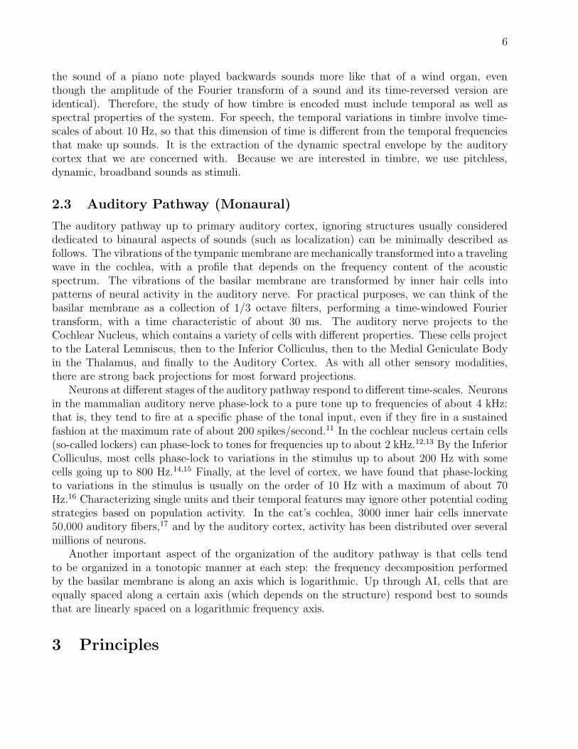
Figure 8: Left: A time slice of the stimulus: 101 tones equally spaced along the logarithmic axis.This ripple has a ripple frequency Ω of 0.4 cyc/oct with zero phase, and a linear modulation of50%, against an arbitrary intensity axis (see Equation (4)). Right: the spectral profile changes as afunction of time, giving a moving ripple, here with positive frequency (since the phase increases asa function of time).

4.1 The Ripple Stimulus

The auditory stimulus we use has a sinusoidal profile at any instant in time. Since it wouldbe hard to generate noise and then shape it with filters, we generate ripples over a range of5 octaves by taking 101 tones with logarithmically spaced (temporal) frequencies and random(temporal) phases. The amplitude S(x, t) of each tone of frequency f , with x = log2(ff0), f0the lower edge of the spectrum, is then adjusted as

S(x, t) = L (1 + ∆A · sin (2π (Ω · x+ w · t) + Φ)) , (4)

for a linear modulation. L is the overall base of the stimulus and is adjusted to a level typically10-15 dB above the lower threshold of the cell as determined with pure tones at the tonal bestfrequency. The overall level of a single-ripple stimulus is calculated from the level of its singlefrequency components: thus, a flat ripple of level L1 is composed of 101 components, each atL1 − 10 log (101) ≈ L1 − 20 dB.

Five parameters are sufficient to characterize the ripple stimulus:

• The ripple frequency Ω in cycles/octave,

• The ripple velocity w in Hz, so that a positive value of w and Ω corresponds to a ripplewhose envelope travels towards the low frequencies

• The level or base loudness of the ripple,

• The amplitude of the modulation ∆A of the ripple around the base,

• The ripple’s initial phase.

Since the tones that make up a ripple are logarithmically spaced, its pitch is indeterminate.

14

0 1 2 3 4 5

0 125 250 375 500

0

Octaves

Time (ms)

Figure 9: The top panel represents the spectral envelope of the stimulus at a given instant againstan arbitrary intensity axis. For the two cells represented in the middle panel (with IR (t) = δ (t)),one (unbroken) with the RF centered on low frequencies (xm = 1, asymmetric with φ = 90o), andthe other (broken) with the RF centered on high frequencies (xm = 4, symmetric with φ = 0o), theexpected responses to a 4 Hz ripple is shown in the bottom panel (unbroken and broken, respec-tively),against some measure of the response, for instance spikes/sec or the intracellular potential.In our case, the actual response is half-wave rectified, and measured in the form of a spike count,so that the bottom panel should really be seen as a spiking probability that can be measured bymeasuring the response of the cell to many presentations of the same stimulus.

4.2 Data Analysis

In this section, we show the data analysis we apply with the help of a simulation, but to keepthe graphs one-dimensional we assume that in Figure 9 and Figure 10, IR (t) = δ (t).

We use two paradigms to obtain the transfer function of a cell. First, we choose a ripplefrequency and present the cell with ripples of varying ripple velocities (typically, -24 Hz to 24Hz in cortex). Then, for a fixed ripple velocity, we present the cell with ripples of varying ripplefrequencies (typically, from -1.6 to 1.6 cyc/oct).

As indicated for a 4 Hz ripple in Figure 9, the response of a cell as a function of time ismodulated at the same (temporal) frequency as that of the stimulus. Therefore, we just haveto extract the phase and the amplitude of the response. The resulting transfer function for thesame two cells is shown in Figure 10. We have presented ripples to the idealized cells shown inpanel B. The amplitude of the response as a function of ripple frequency is shown in panel C,whereas the phase of the response is shown in the bottom panel. Note that the phase interceptφ is 0o for the symmetric cells and 90o for the antisymmetric cell.

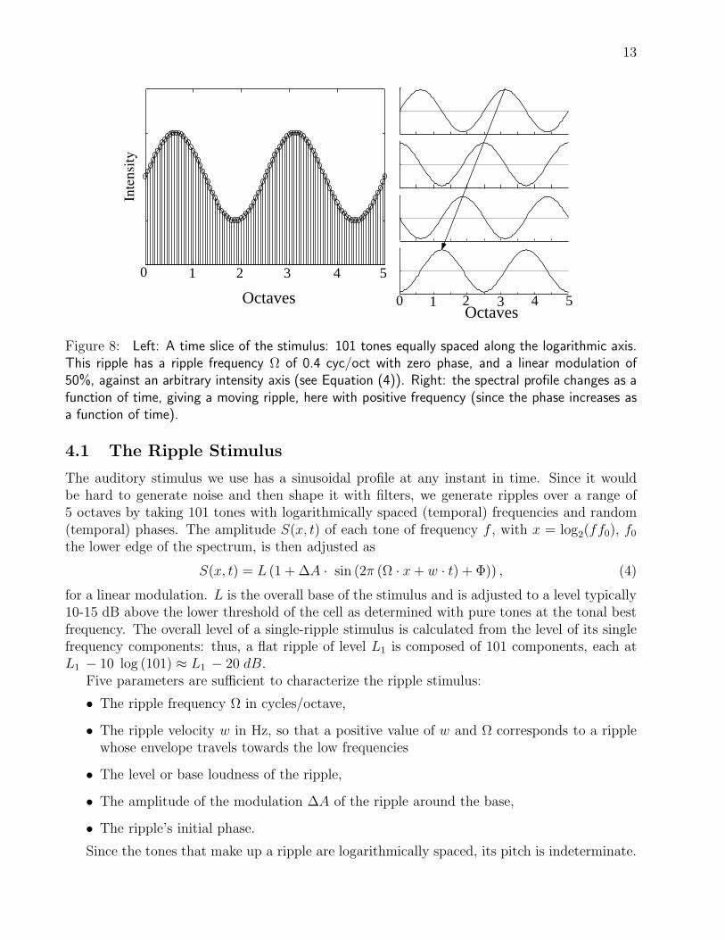
In the corresponding Ω−−w space, the ripple of Figure 8 corresponds to a pair of points.Therefore, to measure the complete ripple response transfer function of a cell we need to measureits response to all possible ripples, as shown in Figure 11. Note that since cells in cortex respond

15

0 1 2 3 4 5

0 1 2 3 4 5

0

0 0.4 0.8 1.2 1.6 2

0 0.4 0.8 1.2 1.6 200.1

π5 π

2 π

Octaves

Cycles/octave

A

B

C

D

0.2

Figure 10: The sounds with the spectrum shown in A (ripples with ripples frequencies of 0 (flatspectrum), 0.4 and 0.8 cycles/octave) are presented at various phases to the two cells in B, asin Figure 9. The amplitude (for instance in spikes/sec) (C) and phase (D) of the best fit to theresponse are shown.

only to transient stimuli, it is not necessary to present the stimuli along the w = 0 axis.

4.3 Separability

We have shown previously16,22 that within each quadrant, actual ripple transfer functions areseparable 5: for two fixed values of Ω, the transfer function as a function of w only changesbetween the two by an overall scale factor and an overall phase. The same is true when Ω andw are reversed. Hence, one is required only to study two lines in Ω − w space. Therefore weonly need to sample a line in each direction within each quadrant, as shown in Figure 12.

Without separability, whether full or quadrant, it would be extremely difficult to characterizea cell by its transfer function. Experimentally, given the time required to measure one pointof the transfer function, measuring the transfer function at the points indicated in Figure 12 isfeasible, whereas measuring the transfer function at all the points indicated in Figure 11 is not.

5Strictly speaking, we have shown it only for the first quadrant, i.e. for down-moving ripples.

16

w

Ω

Figure 11: To measure the complete ripple transfer function, we have to measure the responseof the cell to all the ripples represented by large circles above. The smallest circles correspond toredundant ripples, as inspection of Eq. (2) and Figure 5 shows.

w

Ω

Figure 12: Since we found experimentally that cells have separable transfer functions within eachquadrant, it is enough to measure the transfer function along two orthogonal lines in each quadrant.

4.4 Linearity

Linearity is confirmed by comparing the response to combinations of ripples with the responsepredicted by summing the responses to the individual ripples, i.e. the values of the transfer func-tion. A combination of ripples is computed such that its base loudness is the same as the individ-ual ripples’, and the amplitude of the modulation is scaled as in Equation (4). As an example, topresent the combination of two ripples (whose properties are described by subscripts 1 and 2), wecompute B = B1 sin (2π (Ω1 · x+ w1 · t) + Φ1) +B2 sin (2π (Ω2 · x+ w2 · t) + Φ2). For a mod-ulation of ∆A, the envelope is (in the manner of Equation (4)) L ·(1 + ∆A · B/max (B)), whereL is the base intensity level. The sound is generated from the envelope using 101 tones over 5octaves with logarithmically spaced (temporal) frequencies and random (temporal) phases.

17

5 Experiment and Results

5.1 Experimental Details

Data were collected from domestic ferrets (Mustela putorius). The ferrets were anesthetizedwith sodium pentobarbital and anesthesia was maintained throughout the experiment by con-tinuous intravenous infusion of either pentobarbital or ketamine and xylazine, with dextrose (inRinger’s solution) to maintain metabolic stability. The ectosylvian gyrus, which includes theprimary auditory cortex, was exposed by craniotomy and the dura reflected. The contralateralear canal (meatus) was exposed and partly resected, and a cone-shaped speculum containing aminiature speaker was sutured to the meatal stump. For details on the surgery see Shamma etal3.

All stimuli were computer synthesized, gated, and then fed through a common equalizer intothe earphone. Calibration of the sound delivery system (to obtain a flat frequency response upto 20 kHz at the level of the eardrum) was performed in situ using a 1/8-in. probe microphone.

Action potentials from single units were recorded using glass-insulated tungsten micro-electrodes with 5-6 MΩ tip impedances. Neural signals were fed through a window discriminatorand the time of spike occurrence relative to stimulus delivery was stored on a computer, whichalso controlled stimulus delivery, and created raster displays of the responses. In each animal,electrode penetrations were made orthogonal to the cortical surface. In each penetration, cellswere typically isolated at depths of 350-600 µm corresponding to cortical layers III and IV3.

5.2 Obtaining the Transfer Functions

As explained above, we measure the cells’ transfer functions by presenting first, at a fixed ripplefrequency, ripples of various velocities. Then, for a fixed ripple velocity, we present ripples ofvarying ripple frequencies.

5.2.1 Spectral cross-section of the transfer function

A typical example of the analysis is shown in Figure 13. Ripples were presented at 8 Hz, forripples frequencies from -1.6 cyc/oct to 1.6 cyc/oct in steps of 0.2 cyc/oct, with the ripplestarting to move at t = 0ms, but being acoustically turned on starting at 50 ms with a linearramping over 8 ms. Each action potential is denoted by a dot on the raster plot in A. One cansee the onset response to the ripple at about 70 ms (50 ms + delay due to the ramping up of thestimulus, + latency of the response). Each ripple is presented 15 times. Once the onset activityhas died away, the cell goes into a sort of steady-state response. For each ripple frequency, wecompute a period histogram starting at 120 ms (this excludes the onset response). Four ofthose histograms are shown in panel B. To assess the strength and phase of the phase-lockedresponse, we divide the histogram into 16 equal bins. The amplitude and phase of the responseis then evaluated by performing a Fourier transform of the data, and extracting the phase ofT (Ω, w = 8 Hz) from the first component of the Fourier transform, and the amplitude from

T (Ω, w = 8 Hz) = AC1 (Ω) ·|AC1 (Ω)|

√

∑8i=1 |ACi (Ω)|

2(5)

18

If the modulation of the response were that of a purely linear system, the higher coefficientsACi(Ω) would be negligible. But because of the half-wave rectification and other non-linearities,they usually are significant. Therefore we weight AC1(Ω) by the RMS of the other coefficientsof the ACi(Ω) to assess linearity.

The magnitude and phase of the transfer function is shown in panel C. In D, we have inverseFourier transformed separately the transfer function in quadrant 1 and 2, or equivalently fordown- and up-moving ripples, after removing the constant (temporal) phase factor 2πwτd + θ,where w = 8Hz. In this case, the up- and down-moving RFs match very well with each otherand with the RF obtained with a two-tone paradigm3.

Note that the period histograms shown in panel B correspond to periods starting at 120ms, so as to eliminate the effect of the onset response, whereas the second graph in panel Cshows phases sent back to 0 ms, at which point in time the phase of the ripples presented wereall 0 degrees.

5.2.2 Temporal Cross-Section of the Transfer Function

An example of the extraction of the temporal cross-section of the transfer function for the samecell as in Figure 13 is shown in Figure 14. Ripples are presented at 0.4 cyc/oct, for ripplevelocities from -24 Hz to 24 Hz in steps of 4 Hz, with the ripple starting to move at t = 0ms,being acoustically turned on starting at 50 ms with a linear ramping over 8 ms. Each actionpotential is denoted by a dot on the raster plot in A. One can see the onset response to theripple at about 70 ms (50 ms + delay due to the ramping up of the stimulus, + latency ofthe response). Each ripple is presented 15 times. Once the onset activity dies away, the cellgoes into a steady-state response. For each ripple frequency, we compute a period histogramstarting at 120 ms (so that the onset response is excluded). Four of those histograms are shownin panel B. To assess the strength and phase of the phase-locked response, we divide the periodinto 16 equal bins. The amplitude and phase of the response is then evaluated by performinga Fourier transform of the data, and extracting the phase of T (Ω = 0.4 cyc/oct, w) from thefirst component of the Fourier transform, and the amplitude from

T (Ω = 0.4 cyc/oct, w) = AC1 (w) ·|AC1 (w)|

√

∑8i=1 |ACi (w)|

2(6)

If the modulation of the response were that of a purely linear system, the higher coefficientsACi(w) would be negligible. But because of the half-wave rectification and other non-linearities,they usually are significant. Therefore we weight AC1(w) by the RMS of the other coefficientsof ACi(w) to assess linearity.

The magnitude and phase of the transfer function is shown in panel C. In D, we have inverseFourier transformed separately the transfer function in quadrant 1 and 2, or equivalently fordown- and up-moving ripples, after removing the constant (spectral) phase factor 2πΩxm + φ,where Ω = 0.4 cyc/oct. In this case, the up- and down-moving IRs match very well with eachother.

19

Transfer FunctionAmplitude

0

20

40

-1.6 -0.8 0 0.8 1.6−16 π−8 π

08 π

16 π

Ripple Frequeny (cyc/oct)

C

Transfer FunctionPhase

0

40 0 cyc/oct

0

40

-0.2 cyc/oct

0

200.2 cyc/oct

0

400.4 cyc/oct

0 25 50 75 100 125Time (ms)

B

0RF (Positive Freqs)

RF (Negative Freqs)

0 1 2 3 4 50

40

80

RF (Pure Tones)

0

5

5

Octaves

D

Am

plitu

deS

pike

cou

nt

70 dBRipple Frequency (cyc/oct) Ripple Velocity is 8 HzA

220/

38a0

6

Am

pl

it

ud

e

in

s

pi

ke

s/

bi

n

Figure 13: Data analysis using ripples of fixed velocity and varying frequencies. A: Raster plot ofresponses. Each point represents an action potential, and each paradigm is presented 15 times. B:Period histogram for 4 ripple frequencies. Note how the position of the peak of the best fit changeslinearly with ripple frequency. C: Magnitude and phase of the period histogram fits. D: Separateinverse Fourier transforms for positive and negative ripple frequencies of C, obtaining a slice of theRF. Also given for comparison is the response area as determined by the two-tone paradigm. 3

20

-6

0

6 IR (positive freqs)

0 50 100 150 200 250-6

0

6IR (negative freqs)

Time (ms)

D

-24 -16 -8 0 8 16 24

0

20

−2 π

−π

Ripple velocity (Hz)

C Transfer FunctionAmplitude

Transfer FunctionPhase

0

20 -12Hz

0 60 804020

0

40 -8Hz

0 75 100 1255025

0

80 -4Hz

0 150 200 25010050

0

8 0 Hz

0 1700Time (ms)

B

70 dBARipple Velocity (Hz) Ripple Frequency is 0.4 cyc/oct

Figure 14: Data analysis using ripples of fixed frequency and varying velocities. A: Raster plotof responses. Each point represents an action potential, and each paradigm is presented 15 times.B: Period histogram for 4 ripple velocities. Note how the peak of the best fit changes linearly withripple velocity (the 0 Hz case can be used to estimate noise). C: Magnitude and phase of the periodhistogram fits. D: Separate inverse Fourier transforms for positive and negative ripple velocities ofC, obtaining a slice of the IR.

21

w = 4 Hz w = 8 Hz w = 12 Hz

0.5 1 2 4 8 16-20

0

20

40

60

wm = 8 Hz

ρ 4,8 = 0.93ρ 12,8 = 0.99

ARF (x) Positive Frequencies

0 100 200 300 400 500

-4

0

4

Ωm = 0.4 cyc/oct

ρ 0.4, 0.8 = 0.89

ρ 0.4, 0.2 = 0.92

B

Time (ms)

Ω = 0.4 cyc/oct Ω = 0.8 cyc/oct Ω = 0.2 cyc/oct

IR(t) Positive Frequencies

Frequency (kHz)

Figure 15: Left The positive-frequency RF computed at constant ripple velocity for 3 differentripple velocities. The shapes should be the same if the system is separable. Right The positive-frequency IR at constant ripple frequency for 3 different ripple frequencies. The shapes should bethe same if the system is separable.

5.3 Quadrant Separability

RF (x) and IR(t), as illustrated in panels D of Figure 13 and Figure 14, are linear combina-tions of the transfer function evaluated along cross-sections of the Ω − w plane. Constancyof RF (x) computed for different w is equivalent to proportionality of T (Ω, w) for different w(and similarly for RF (x), Ω, and T (Ω, w)). This was the requirement given above to verifyquadrant separability. This has all been verified for many cells in the first quadrant16. While itis theoretically possible for the remaining independent quadrant to be nonseparable, it seemsunlikely in ferrets, humans, and most mammals (possible exceptions might include sonar-usinganimals, which could require further specialization). We are currently verifying separability inthe second quadrant.

Shown in Figure 15 are examples of the positive-frequency RF and positive-frequency IRfor two cells, as computed at the different sections indicated.

5.4 Quadrant Linearity

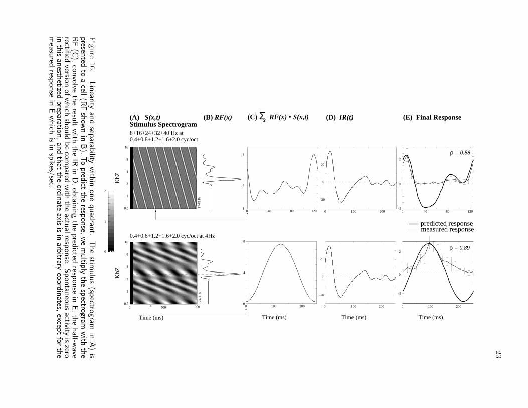
Linearity has been verified by presenting cells with a combination of ripples from differentquadrants16,22,23. As shown in Figure 16 for one cell, the correlation between the predicted andthe measured response is (as in most cases) very good. Note that the predicted response isshown in its non-half-wave rectified version: as cells do not have negative firing rates, and thepentobarbital anesthetic has reduced the spontaneous activity to zero, the comparison should bemade between the actual response and the half-wave rectified version of the predicted response.The correlation coefficient ρ in Figure 16 is the cross-correlation between the measured andthe predicted response. We have previously presented the correlation between prediction andresponse within a single quadrant for 55 cells and found 84% of the cells with ρ > 0.6.22 The

22

error bars on the measured response show the variability of cortical cells’ responses from sweepto sweep. Disparity is maximal between the prediction and the actual spike count where bothare small.

5.5 Full-Quadrant Separability and Linearity

The remainder of this discussion describes logical extensions that are currently under study.Thus far we have only verified separability in a single quadrant. In vision, some cortical simplecells are fully separable24, but all are at least quadrant separable25. We have found both typesin the auditory cortex as well; Figure 17 shows examples of each. A fully separable cell has anSTRF that is a simple product of an RF and an IR, as in A. A quadrant separable cell, as inB, does not, since it has different responses for upward and downward moving ripples (as canbe seen by inspection of its STRF (x, t): it is not symmetric about xm). The separability of acell does not affect the linearity of responses to ripple combinations.

5.6 Response Characteristics

The transfer function for a specific cell is typically tuned to a characteristic ripple frequencyand velocity. The population of cells shows a wide range of characteristic ripple frequencies andvelocities. Characteristic ripple velocities are mostly in the 8 - 16 Hz range, rarely exceeding30 Hz, and characteristic ripple frequencies are mostly in the 0.4 - 0.8 cycles per octave range,rarely exceeding 2 cycles per octave (in this anesthetized preparation). The slope of the transferfunction as a function of ripple frequency, xm, corresponds to the center frequency of the spectralenvelope, which ranges from 200 Hz to at least 24 kHz (above which our acoustic delivery systemis inadequate). The slope of the transfer function as a function of ripple velocity, τd, correspondsto the center of the temporal envelope, which ranges roughly from 10 ms to 60 ms. The RFsymmetry φ, which describes the effects of lateral inhibition and excitation, ranges roughlyfrom −90o to +90o (out of a possible −180o to +180o), clustered around 0o. The IR polarityθ, which describes the polarity of the temporal response, ranges roughly from 45o to 135o (outof a possible 0o to 180o).

6 Conclusions

The emphasis in this review has been on presenting a technique to describe neural responsepatterns of units in the cortex. More precisely, we use moving ripples to characterize theresponse fields of auditory cortical neurons, although this is a general method that can be usedanywhere responses are shown to be substantially linear for broadband stimuli.

Practically, we find that because of linearity of cortical responses with respect to spectralenvelope, we can use the ripple method to characterize auditory cortical cell responses todynamic, broadband sounds. The linearity of the cortical unit responses is quantified by thecorrelation coefficient between the predicted and the measured responses curves. While atthis point we do not have statistics to quantify the linearity of response to ripples moving inboth directions, linearity within one quadrant (to down-moving ripples) has been extensivelyquantified22, and we have no reason to expect linearity be any different for ripples moving in

23

2

0

-20 40 80 120

ρ = 0.88

2

0

-2

2001000

ρ = 0.89

(E) Final Response

predicted responsemeasured response

Time (ms)

2001000

-20

0

20

20

0

-20

0 100 200

(D) IR(t)

Time (ms)

1

4

8

0 40 80 120

(A) S(x,t)Stimulus Spectrogram

(B) RF(x) (C) Σx RF(x) . S(x,t)

8+16+24+32+40 Hz at0.4+0.8+1.2+1.6+2.0 cyc/oct

174/

11b

16

8

4

2

1

0.5

KhZ

0 100 2000

4

8

Time (ms)

174/

11b

1000500

Time (ms)

0

0.4+0.8+1.2+1.6+2.0 cyc/oct at 4Hz16

8

4

2

1

0.5

KhZ

0

1

2

Figu

re16:

Linearity

andsep

arability

with

inonequadran

t.Thestim

ulus(sp

ectrogramin

A)is

presented

toacell

(RFshow

nin

B).Topred

icttheresp

onse,

wemultip

lythespectrogram

with

the

RF(C

),con

volvetheresu

ltwith

theIR

inD,obtain

ingthepred

ictedresp

onse

inE,thehalf-w

averectifi

edversion

ofwhich

should

becom

pared

with

theactu

alresp

onse.

Spontan

eousactivity

iszero

inthisanesth

etizedprep

aration,andthat

theord

inate

axisisin

arbitrary

coord

inates,

exceptfor

the

measu

redresp

onse

inEwhich

isin

spikes/sec.

24

=

=

t*-50

0

50

.25

.5

1

2

4

8

B

0.25

0.5

1

2

4

8STRFStimulus SpectrogramA

time (ms)0 100 200

1

2

4

8

0.5

16

0 100 200

1

2

4

8

0.5

16

-20

0

20

time (ms)0 100 200

time (ms)

Response

PredictionResponse

Spike rate=0Spontaneous

t*F

requ

ency

(kH

z)F

requ

ency

(kH

z)

222/

14a0

7(13

)21

9/21

b06(

11)

Figure 17: Predictions of responses to complex dynamic spectra using the STRF. A The predictedresponse is computed by a convolution (along the time dimension) of the STRF with the spectrogram.The stimulus shown is composed of two ripples (0.4 cycles/octave at 12 Hz and -4 Hz). The predictedwaveform is shown juxtaposed to the actual response (crosses) over one period of the stimulus, inspikes/bin summed over 30 sweeps. B Another example: the stimulus consists of a combinationof ripples with ripple frequencies 0.2 cycles/octave at 4 Hz, 0.4 cycles/octave at 8 Hz, ... 1.2cycles/octave at 24 Hz, in cosine phase, resulting in an FM-like stimulus. In this Ketamine/Xylazinepreparation, the spontaneous activity was non-zero.

both directions. The separability of cells makes the ripple method practical, because of thetime needed to characterize a cell. One advantage of the method is the simultaneous probingof spectral and temporal characteristics. Temporal processing is becoming more and morerecognized as an essential part of cortical function, and the ripple method places it on an equalfooting with spectral processing. A caveat is that, thus far, the method only has been appliedto the steady state (i.e. periodic) response of cells.

We find that response fields in AI tend to have characteristic shapes both spectrally andtemporally. Specifically, AI cells are tuned to moving ripples, i.e., a cell responds well onlyto a small set of moving ripples around a particular spectral peak spacing and velocity. Wefind cortical cells with all center frequencies, all spectral symmetries, bandwidths, latencies andtemporal impulse response symmetries. One way to interpret this result is that AI decomposesthe input spectrum into different spectrally and temporally tuned channels. Another equivalentview is that a population of such cells, tuned around different moving ripple parameters, caneffectively represent the input spectrum at multiple scales. For example, spectrally narrow cellswill represent the fine features of the spectral profile, whereas broadly tuned cells represent thecoarse outlines of the spectrum. Similarly, dynamically sluggish cells will respond to the slowchanges in the spectrum, whereas fast cells respond to rapid onsets and transitions. In this

25

manner, AI is able to encode multiple different views of the same dynamic spectrum. From this,we conclude that the primary auditory cortex performs multi-dimensional, multi-scale wavelettransform of the auditory spectrum.

Pitch is very important to the auditory system. The spectral ripple responses presentedhere do not have pitch, since they are synthetized with logarithmically spaced carrier tones.We have not yet examined unit responses to a ripple spectra with harmonically related carriertones. Consequently, all our unit responses are due to the envelope or spectral profile of thebroadband stimulus, and are not dependent on the carrier tones. It is quite possible that thepitch of a harmonic series of tones will affect the responses. It is also possible that sufficientlynarrowly tuned cells might directly encode the harmonic spacing in a spectrum in a systematicmanner to encode the pitch as was discussed in detail in Wang and Shamma26. This is work inprogress.

The suggestion that cortical cells are linear might appear far-fetched given the non-linearresponse to pure tones, such as rate vs. intensity functions with threshold, saturation, andnon- monotonic behavior (Brugge and Merzenich27; Nelken et al.8). Nevertheless, we findthat the non-linearity observed with broadband ripple spectra is substantially smaller thanwith tonal stimuli, when it comes to predicting the response of a cell to a combination ofstimuli, knowing the response to individual ones. Furthermore, just as measuring linear systemsresponse properties with tones, such as bandwidth, rate-level functions, tuning quality factorand other measures is considered meaningful, characteristics of the ripple responses prove useful,and relate to the properties measured with tones18,16. Investigations currently under way inthe Inferior Colliculus will shed light on the mechanisms that allow cells to exhibit a linearbehavior in auditory cortex, so many synapses away from the auditory nerve.

7 Acknowledgements

This work is supported by a MURI grant N00014-97-1-0501 from the Office of Naval Research,a training grant NIDCD T32 DC00046-01 from the National Institute on Deafness and OtherCommunication Disorders, and a grant NSFD CD8803012 from the National Science Founda-tion. We would like to thank David Klein, Izumi Ohzawa and Alan Saul.

8 References

1. M.M. Merzenich, P.L. Knight and G.L. Roth, Representation of the cochlear partition on thesuperior temporal plane of the macaque monkey, Brain Res. 50, 231-249 (1975). R.A. Reale andT.J. Imig, Tonotopic organization in auditory cortex of the cat, J. Comp. Neurol. 192, 265-291(1980).

2. J.C. Middlebrooks, R.W. Dykes and M.M. Merzenich, Binaural response-specific bands in primaryauditory cortex of the cat: topographical organization orthogonal to isofrequency contours, BrainRes. 181, 31-48 (1980).

3. S.A. Shamma, J.W. Fleshman, P.R. Wiser and H. Versnel, Organization of response areas in ferretprimary auditory cortex, J. Neurophys. 69, 367-383 (1993).

4. C.E. Schreiner, J. Mendelson and M.L. Sutter, Functional topography of cat primary auditorycortex: representation of tone intensity, Exp. Brain Res. 92, 105-122 (1992).

26

5. C.E. Schreiner and M.L. Sutter, Topography of excitatory bandwidth in cat primary auditorycortex: single- versus multiple-neuron recordings, J. Neurophysiol. 68, 1487-1502 (1992).

6. J. Mendelson, C.E. Schreiner, M.L. Sutter and K. Grasse, Functional topography of cat primaryauditory cortex: selectivity to frequency sweeps, Exp. Brain Res. 94, 65-87 (1993).

7. R.L. De Valois and K.K. De Valois, Spatial Vision, Oxford University Press, New-York (1988).8. I. Nelken, Y. Prut, E. Vaadia and M. Abeles, Population responses to multifrequency sounds in

the cat auditory cortex: One- and two-parameter families of sounds, Hear. Res. 72, 206-222 (1994).9. M.L. Sutter,.W.C. Loftus and K.N. O’Connor, Temporal properties of two-tone inhibition in cat

primary auditory cortex, ARO midwinter meeting (1996).10. L.R. Rabiner and R.W. Schafer, Digital processing of speech signals, Prentice-Hall, New-Jersey

(1978).11. J.E. Rose, J.F. Brugge, D.J. Anderson and J.E. Hind, Phase-locked response to low-frequency

tones in single auditory nerve fibers of the squirrel monkey, J. Neurophys. 30, 769-793 (1967).12. W.S. Rhode and P.H. Smith, Encoding time and intensity in the central cochlear nucleus of the

cat, J. Neurophys. 56, 262-286 (1986).13. W.S. Rhode and S. Greenberg, Physiology of the cochlear nuclei, in The mammalian auditory

pathway: Neurophysiology, Popper, A.N. and Fay, R.R. editors, Springer-Verlag, New-York (1991).14. R. Lyon and S.A. Shamma, Timbre and pitch, in Auditory computation, H.L. Hawkins., T.A.

McMullen, A.N. Popper and R.R. Fay, editors, Springer-Verlag, New-York (1995).15. G. Langner, Periodicity coding in the auditory system, Hearing Res. 6, 115-142 (1992). D.A.

Depireux, D.J. Klein, J.Z. Simon and S.A. Shamma, Neuronal correlates of pitch in the InferiorColliculus, ARO midwinter meeting (1997).

16. N. Kowalski, D.A. Depireux and S.A. Shamma, Analysis of dynamic spectra in ferret primaryauditory cortex: I. Characteristics of single unit responses to moving ripple spectra, J. Neurophys.76, (5) 3503-3523 (1996).

17. D.K. Ryugo, The auditory nerve: peripheral innervation, cell body morphology, and central pro-jections, in The mammalian auditory pathway: neuroanatomy, D.B. Webster, A.N. Popper, andR.R. Fay, editors, Springer-Verlag, New-York, (1991).

18. C.E. Schreiner and B.M. Calhoun, Spatial frequency filters in cat auditory cortex. Auditory Neu-rosci. 1, 39-61 (1994). S.A. Shamma, H. Versnel and N. Kowalski, Ripple analysis in ferret primaryauditory cortex: I. Response characteristics of single units to sinusoidally rippled spectra. Audi-tory Neurosci. 1, 233-254 (1995). S.A. Shamma and H. Versnel, Ripple analysis in ferret primaryauditory cortex: II. Prediction of unit responses to arbitrary spectral profiles. Auditory Neurosci.1, 255-270 (1995). H. Versnel, N. Kowalski and S.A. Shamma, Ripple analysis in ferret primaryauditory cortex: III. Topographic distribution of ripple response parameters. Auditory Neurosci.1, 271-285 (1995).

19. A. Papoulis, The Fourier integral and its applications, McGraw-Hill (1962).20. L. Cohen, Time-frequency analysis, Prentice-Hall, New Jersey (1995).21. D. Dong and J.J. Atick, Temporal decorrelation: a theory of lagged and nonlagged cells in the

lateral geniculate nucleus, Network: Computation in Neural Systems 6, 159-178 (1995).22. N. Kowalski, D.A. Depireux and S.A. Shamma, Analysis of dynamic spectra in ferret primary

auditory cortex: II. Prediction of unit responses to arbitrary dynamic spectra. J. Neurophys. 76,(5) 3524–3534 (1996).

23. J.Z. Simon, D.A. Depireux and S.A. Shamma, Representation of complex dynamic spectra inauditory cortex, in Psychophysical and physiological advances in hearing, A.R. Palmer, A.Rees,A.Q. Summerfield and R. Meddis, editors, Whurr Publishers, London (1988).

24. J. McLean and L.A. Palmer, Organization of simple cell responses in the three-dimensional fre-

27

quency domain. Vis. Neurosc. 11, 295-306 (1994). G.C. DeAngelis, I. Ohzawa and R.D. Freeman,Receptive-field dynamics in the central visual pathways. Trends Neurosc. 18, 451-458 (1995).

25. B.W. Andrews and D.A. Pollen, Relationship between spatial frequency selectivity and receptivefield profile of simple cells, J. Physiol. (London) 287, 163-176 (1979). S.M. Friend and C.L. Baker,Spatio-temporal frequency separability in area 18 neurons of the cat, Vision Res. 33, 1765-1771(1993).

26. K. Wang and S. A. Shamma, Self-normalization and noise robustness in auditory representations.IEEE Trans. Audio. Speech. Proc. 2, 421-435 (1994).

27. J. F. Brugge and M. M. Merzenich, Responses of neurons in auditory cortex of the Macaquemonkey to monaural and binaural stimulation. J. Neurophysiol. 36, 1138-1158 (1973).