Measuring the Economic Impact of Civil War

Kosuke Imai and Jeremy Weinstein

CID Working Paper No. 51June 2000

Copyright 2000 Kosuke Imai and Jeremy Weinsteinand the President and Fellows of Harvard College

This paper can be downloaded in PDF format from:http://www.cid.harvard.edu/cidwp/051.pdf

Measuring the Economic Impact of Civil War

Jeremy M. Weinstein and Kosuke Imai

Abstract

Civil wars impose substantial costs on the domestic economy. We empiricallymeasure the economic impact of such internal wars. The paper contributes to the existingliterature both theoretically and methodologically. First, it explores the economicchannels through which civil war affects growth. Previous studies have shown thenegative growth effects of civil wars. We go a step further by identifying the channelsthrough which war strips a country of its growth potential. Our argument is that civil warnegatively impacts private investment through the process of portfolio substitution.

Methodologically, the paper improves on both the data and statistical models used in theexisting literature. Our data set includes better measurements of the intensity and scope ofcivil war as well as new economic and political data for the 1990s. Moreover, using amultiple imputation technique, we minimize the estimation bias due to missing data.Finally, to improve the model, we apply fixed and random effects models to the paneldata.

The evidence gives strong support to our argument indicating that the driving forcebehind the negative effects of civil war on economic growth is a decrease in privateinvestment.

Keywords: civil war, instability, economic growth, investment, fiscal balance

JEL codes: C23, E62, O11

Jeremy M. Weinstein is a PhD Candidate in Political Economy and Government atHarvard University. He is a Graduate Student Fellow of the Center for InternationalDevelopment and his research focuses on the intersection between political instabilityand economic development.

Kosuke Imai is a Ph.D. candidate in the Department of Government at HarvardUniversity. His interests include empirical methodology and political economy of war.

Contents

1 Introduction 1

2 Theory and Hypotheses 32.1 Effect through domestic investment . . . . . . . . . . . . . . . . . . . . . . . . . . . . 32.2 Effect through fiscal policy . . . . . . . . . . . . . . . . . . . . . . . . . . . . . . . . 52.3 Differentiating civil war . . . . . . . . . . . . . . . . . . . . . . . . . . . . . . . . . . 6

3 Existing Evidence 73.1 Growth effect of civil war . . . . . . . . . . . . . . . . . . . . . . . . . . . . . . . . . 73.2 Fiscal deficit effects of instability . . . . . . . . . . . . . . . . . . . . . . . . . . . . . 8

4 Empirical Analysis 84.1 Data . . . . . . . . . . . . . . . . . . . . . . . . . . . . . . . . . . . . . . . . . . . . . 84.2 Result 1: Growth effect . . . . . . . . . . . . . . . . . . . . . . . . . . . . . . . . . . 104.3 Result 2: Effect through investment . . . . . . . . . . . . . . . . . . . . . . . . . . . 114.4 Result 3: Effect through fiscal policy . . . . . . . . . . . . . . . . . . . . . . . . . . . 13

5 Improving Estimation 135.1 Multiple imputation method . . . . . . . . . . . . . . . . . . . . . . . . . . . . . . . . 145.2 Models for panel data . . . . . . . . . . . . . . . . . . . . . . . . . . . . . . . . . . . 145.3 Results . . . . . . . . . . . . . . . . . . . . . . . . . . . . . . . . . . . . . . . . . . . . 16

6 Reinterpretation of the Model Prediction 18

7 Conclusion 20

A Data description 22

B Replication of Collier(1999) 24

C Note on multiple imputation procedure 25

i

1 Introduction

Civil wars impose substantial costs on the domestic economy.1 These wars are destructive of human

lives and economic infrastructure. They also undermine the legitimacy of the state, threatening its

institutions, the security of property rights, and the rule of law. Moreover, internal wars introduce

tremendous uncertainty into the economic environment, making both public and private investment

riskier. While it might be readily apparent that war will impact economic production, there is little

understanding about the different channels through which civil war affects the aggregate economy.

How costly are these internal wars? What is the mechanism through which civil war negatively

impacts the domestic economy? Building on the emerging literature on the economics of civil war,

this paper measures the economic costs of war and identifies the ways in which civil war strips a

country of its growth potential.

This paper contributes to the existing analysis both theoretically and methodologically. In

particular, we explore the economic channels through which civil war affects growth by investigating

two theoretical arguments. First, civil war impacts the domestic economy by reducing the level

and growth of the capital stock. The occurrence of civil war initiates capital flight and thus

dramatically reduces private investment. Second, political economy models suggest that internal

conflicts affect the aggregate domestic economy by worsening the government’s fiscal balance.

Economically, governments shift expenditure from output enhancing activities into the conduct

of war. Politically, they face weaker incentives to maintain fiscal balance owing to a shorter time

horizon and weaker accountability to an electoral constituency. We directly test these two potential

explanations. Our results indicate that the driving force behind the negative effects of civil war on

economic growth is a decrease in domestic investment, and in particular, private investment.

The second goal of this paper is to provide a better measurement of the economic impacts of

civil war. To do so, we investigate the characteristics of civil war that are the most damaging for

the domestic economy. Civil wars vary tremendously in their scope. Some wars are fought entirely

in one region of the country, while in others the fighting extends throughout the countryside and

into urban areas. Some civil wars may involve high levels of civilian fatalities as in Sierra Leone,1We define civil wars to include both revolutionary wars, in which one group aims to overthrow the state or

establish control of an autonomous region, and ethnic conflicts, in which the government engages in armed conflictwith a national, ethnic, or religious minority. A more complete definition of civil war is included in Appendix A.

1

Mozambique, and Guatemala, while others may be fought largely between competing militaries. In

our empirical analysis, we find that the scope of the civil war significantly influences the magnitude

of the economic effects. Wars that spill out across the entire country, require the highest level of

military recruitment, and result in the greatest number of fatalities are the most damaging to the

domestic economy.

This paper also makes methodological improvements. First, we improve the data. The data

set used in the existing literature on the economic consequences of civil war contains a number of

missing observations despite the fact that it relies on the decade-average of economic indicators.

A significant problem is that these observations are not missing completely at random. In our

sample, the listwise deletion of missing observations leads to significant over-representation of war-

decades. Such non-random missing data is likely to bias the result of analysis. We utilize a multiple

imputation program developed by King et al. (2000) in order to exploit all available information.

The empirical analysis based on this improved data set gives a more accurate assessment of the

economic effects of civil war.

Second, we improve the model. The existing empirical literature exploring political influences

on growth has often applied a pooled Ordinary Least Squares to panel data. However, this approach

is problematic in that it ignores country specific effects, possibly leading to biased results. In this

paper, we test the robustness of our pooled OLS results by applying appropriate panel data models

to the analysis of economic growth and political conflicts.

Finally, we improve the interpretation of our statistical models following the suggestion of King

et al. (2000). We show that researchers often underestimate the uncertainty of the model prediction.

Economic data is by nature so noisy that many models fail to capture its dynamic structure.

Interpretation of the statistical results produced by such a model requires special caution. Whereas

researchers often pay attention to the estimation uncertainty around the coefficient, it is necessary

that we also take into consideration the fundamental uncertainty that remains unexplained by the

poorly-fit model. We use simulation to show how ignoring the fundamental uncertainty can result

in incorrect interpretation of statistical results.

In the next section, we set out the theoretical framework. Section 3 examines the existing evi-

dence in the literature. In section 4, we analyze a set of new economic and conflict-related variables

to conduct a direct test of our theory. Section 5 improves the estimation by using a multiple im-

2

putation technique to replace missing observations and by introducing different statistical models.

Section 6 estimates fundamental uncertainty of the model and reinterprets the results. Section 7

gives our conclusion.

2 Theory and Hypotheses

First, we examine the general hypothesis that civil war negatively impacts economic growth

(Knight, Loayza, and Villanueva 1996; Easterly and Levine 1997; Collier 1999).

Hypothesis 1 (Growth Hypothesis) Civil war has a negative impact on economic growth.

The main purpose of this paper is to explore the channels through which civil war affects the

domestic economy. In the following sections, we develop hypotheses about two potential sources

of the growth collapse: reduction in domestic investment and negative effects on the government

fiscal balance.

2.1 Effect through domestic investment

The capital stock of an economy represents its accumulated stock of residential structures, ma-

chinery, factories, and equipment that exist at a point in time and add to the productive power of

the economy. Increases in the capital stock are a crucial source of economic growth. Neo-classical

growth theory suggests that changes in the capital stock come from two sources: investment and

depreciation.

Change in the capital stock = I − dK

Civil war affects the capital stock in two ways. First, internal conflict reduces the existing stock

of capital. Residential structures, roads, bridges, ports, and factories are targeted and destroyed

by competing militaries in wartime. The level of the capital stock is also affected over time by

changes in investment and the rate of depreciation. In order for the capital stock to grow, the

level of investment in the maintenance and expansion of the capital stock must outpace the rate of

depreciation on the existing stock. Since civil war increases the rate of depreciation and reduces

3

investment, growth in the capital stock is stunted. Civil war, therefore, reduces both the level of

the capital stock and its rate of growth.

This suggests that a major way in which civil war affects the economy is through dramatic

reductions in domestic investment. According to this perspective, the flight of capital is the driving

force behind the economic costs of conflict. For example, Collier (1999) develops a model of

economic output that distinguishes between liquid and fixed capital. The distinction is that the

former is likely to be responsive to changes in the economic environment, while fixed capital such

as supplies of land, buildings, and unskilled labor is unlikely to move easily even as the economic

environment deteriorates. His model shows that the destructive effects of civil war reduce the stock

of potentially mobile capital.

The mechanism of this argument can be explained as follows. Holders of potentially liquid

capital must compare the marginal returns to their investments in-country relative to the acquisition

of foreign assets. Since civil war reduces the productivity of factors in production, this lowers the

rate of return on investments made in the domestic economy. Further, the destructive effect of

civil war increases the rate of depreciation. Again, this reduces the rate of return on domestic

investments. These effects encourage portfolio substitution from domestic to foreign investment.

Therefore, the implication of Collier’s argument is that civil war has a negative impact on economic

output as assets are shifted away from domestic investment.

Domestic investment has two components: private and public investment. Investment, from

both the private and public sector, is used to maintain and increase the capital stock. Civil war

increases uncertainty in the economic environment and, consequently, investment in domestic assets

becomes riskier. Private agents are more responsive to these changes and better able to substitute

away from domestic assets in their portfolios. Private investment suffers as people save less due to

shorter time horizons and liquid assets are shifted out of the country.

The effect on public investment is more ambiguous. Governments shift their expenditures

away from investment in the capital stock towards the maintenance and expansion of the military.

This suggests that negative changes in overall levels of domestic investment will be driven by both

private and public investment. However, the level of public investment depends on the government’s

ability to access international loans. This is particularly true in poor countries, where most civil

wars take place. If a government was in political hot-water before the conflict began, its access

4

to international capital markets would already have been limited. As a result, the occurrence of

a civil war might not reduce a government’s capacity to invest in the capital stock. Two testable

hypotheses follow from this theoretical perspective.

Hypothesis 2 (Gross Investment Hypothesis) Civil war negatively affects the domestic econ-omy by reducing gross domestic investment.

Hypothesis 3 (Private Investment Hypothesis) Civil war negatively affects the domestic econ-omy by reducing private domestic investment rather than public investment.

2.2 Effect through fiscal policy

Political economy models present a second channel through which civil war might affect economic

growth. Fischer (1993) argues that a stable macroeconomic framework is not sufficient but neces-

sary for sustainable growth. It is possible that civil war is a cause of poor macroeconomic policy:

high inflation, distorted foreign exchange markets, and large budget deficits.

A large literature has developed that explores political influences on the deficit. Alesina and

Tabellini (1990) show that the greater the probability of not being reelected and the greater the

degree of polarization of two political parties, the larger will be the budget deficit in a model where

the optimal policy is budget balance. Two features are important in this model: instability (the

likelihood that the government will be thrown out of office) and polarization (the degree to which

the other party has different preferences). These two factors create incentives for politicians to

behave myopically and incur large fiscal deficits while in power.

Imagine a civil war with two competing political actors. The incumbent in power faces military

competition from a domestic threat. The stronger this threat is, the more likely the incumbent will

not remain in power. Moreover, civil wars are often fought along ideological lines suggesting that

the opposition is likely to have different preferences from the government. Such a situation creates

strong incentives for deficit spending. A more complex extension would introduce further political

dimensions. As the state is weakened by an internal threat, it often turns on the civilian population,

using tools of coercion to maintain its power. Democratic practices are violated and government

accountability is lessened. In addition, as the conflict expands, the state finds itself resource-

constrained and increases its extraction of revenues from the population. Often, this cannot keep

pace with the rising costs of conflict. The result is that with limited electoral accountability and

5

high resource demands, there is an even stronger incentive to incur large deficits in a society torn

by civil war.

These political economy models imply an additional testable hypothesis. Civil wars negatively

affect the government’s fiscal balance.2 Since fiscal balance, as part of a stable macroeconomic

framework, is a key source of growth, poor fiscal policy may be a channel through which civil war

imposes costs on the economy.

Hypothesis 4 (Fiscal Policy Hypothesis) Civil war negatively affects the domestic economyby increasing the government budget deficit.

2.3 Differentiating civil war

Previous research on the costs of conflict has assumed away variation within the scope of civil

war (Knight, Loayza, and Villanueva 1996; Easterly and Levine 1997). With the exception of

war duration (Collier 1999), the assumption has been that all wars are alike. Casual observation

suggests the implausibility of this claim. Some civil wars are concentrated in a particular geographic

area like the rebellion of the Sendero Luminoso in Peru, while the rest of the economy functions

uninterrupted in bustling urban centers. Other wars are spread throughout the country, involving

massive armies on both sides, and resulting in significant fatalities among the civilian population

as in Mozambique’s deadly 14-year civil war. The economic costs of civil war cannot be adequately

assessed unless we take into account variation within the scope and scale of internal conflict.

We measure the scope and scale of the civil war with a variable for the geographical spread

of the civil war. Civil wars vary significantly in the portion of the country that is affected by

fighting. Some rebellions are centered in rural areas or are even launched from across the border

with very few direct impacts on major cities. This is particularly true in developing countries where

the limited technology of conflict precludes the use of airplanes, boats, and mass road transport,

making the movement of troops difficult for insurgent groups. Other conflicts evolve into wide-

spread wars in which much of the country is disrupted by the fighting. This measure captures the2One might argue that higher deficits and economic crises lead to regime change. Literature in comparative

politics has linked large fiscal deficits to the initiation of civil wars and revolutions. We do not explicitly test forreverse causation in our analysis, because we find no effect of civil war on the level of the deficit. Regardless of thedirection of the causation, both arguments suggest that civil wars should be associated with larger deficits. Theevidence does not support this relationship.

6

different characteristics of civil war according to the hypotheses we have outlined above.3

We include a measure of the degree of geographical spread because its effects are consistent with

our hypotheses on the channels through which civil war negatively affects economic growth. To the

degree that conflict is spread widely across a country, there is very little space for pockets of safe

economic activity. Destruction is widespread and the private economy faces a similarly uncertain

environment across the country. Dissaving and capital flight are rampant. The geographic spread

should also affect public investment and the fiscal balance. When a government needs to fight a

conflict on many fronts, its expenditures on the military must increase.

In sum, we suggest that wide-spread conflict is more destructive of the capital stock, disruptive

of the economy, and drives out investment from the entire country. The economic costs of conflict

are increasing in the scope and scale of the civil war.

Hypothesis 5 (Geographical Spread Hypothesis) Wide-spread civil wars involve larger eco-nomic costs than wars fought in small, concentrated regions.

3 Existing Evidence

3.1 Growth effect of civil war

The study most relevant to this paper is an empirical examination of the economic consequences

of civil war by Paul Collier(1999). He quantifies the effects of civil war on growth both during

the war and in a five-year period after the conflict. Collier combines economic data from the

Penn World Tables with data on civil wars from the Correlates of War Project (Small and Singer

1996). This data set provides a sample of 92 countries of which 19 had civil wars. The dependent

variable is the decade average per capita GDP growth rate of each country. Collier introduces

three variables meant to capture the economic effects of an ongoing war, the legacy of the conflict3Alternative measurements are the number of casualties and the strength of the insurgent groups. First, civil

wars differ in terms of the human toll. In some wars, the fighting is intense with civilians a major target. Conflictsin Nigeria and Mozambique are good examples, where upwards of two million and 100,000 were killed respectively.Others involve little direct conflict between the warring parties, such as the Burmese civil war in which less than10,000 were killed over a ten year period. Second, the strength of the insurgent groups varies widely. Some rebelgroups build a major base of support that spans the population, while others represent minority or regional interests.Although these measurements are interesting, we choose the degree of geographical spread since it fits our theorybest as explained. Note that we run our analyses using other scale variables to capture the level of fatalities and thestrength of the insurgent groups. These variables are described in Appendix. However, whatever specification weuse, our qualitative conclusions remain unchanged.

7

in future decades, and the impact of the length of economic transition following the conflict. The

key finding by Collier related to our question concerns the immediate economic consequences of

war duration. Collier claims that ”During civil war the annual growth rate is reduced by 2.2%. A

15-year civil war would thus reduce per capita GDP by around 30%”(p.175, emphasis in original).4

3.2 Fiscal deficit effects of instability

Another literature relevant to our Fiscal Policy Hypothesis tests the empirical predictions gener-

ated by positive theories of the fiscal deficit. Roubini (1991) and Edwards and Tabellini (1991)

find empirical support in testing for the impact of political instability on the level of fiscal deficits.

Roubini defines political instability as the frequency of any government change and finds a sta-

tistically significant result: greater frequency of government change leads to higher fiscal deficits.

Edwards and Tabellini take the analysis a step further. They find that irregular government change

is associated with an even larger fiscal deficit than regular changes in government. Empirical sup-

port has been found for the relationship between political instability and the level of government

deficits. In this paper, we test whether the theoretical and empirical link extends to the influence

of civil war on fiscal policy.

4 Empirical Analysis

In this section, we test our hypotheses on a comprehensive data set. Our goal is to uncover the

channels through which internal conflict diminishes growth and to explore whether the nature of

conflict influences economic cost.

4.1 Data

We explicitly test for the economic channels through which civil war negatively affects growth,

using the geographical spread of civil war to measure its scope and scale. The social and economic

variables are drawn from the Global Development Network Growth Database of the World Bank4In results presented in Appendix B, we replicate Collier’s analysis and offer a slightly different interpretation

of the result. For now, we briefly point out that the −2.2% annual growth rate that Collier gives as result from ayear-long war is actually the result for the effect of a decade-long war. Furthermore, the effect of a 15-year civil waris −3.4% rather than −30% as he claims. Hence, although civil war has a negative impact on economic growth, thesize of the impact seems much smaller than what Collier reported.

8

(Easterly and Yu 2000). Our civil war variables come from a data set developed by the State

Failure Task Force, which covers civil wars in the period 1960-1996 (Gurr and Harff 1997).

Our data set has two advantages over the data used in the existing literature. First, our civil

war variables are more comprehensive in terms of both time and scope than those in other available

data sets. It captures conflicts that range in scope, including small wars that have been previously

excluded from analysis.5 In addition, we are able to update our data set to include civil wars that

occur in the 1990s. Second, our economic variables also cover a longer time period and include

additional variables that are not included in previous studies.

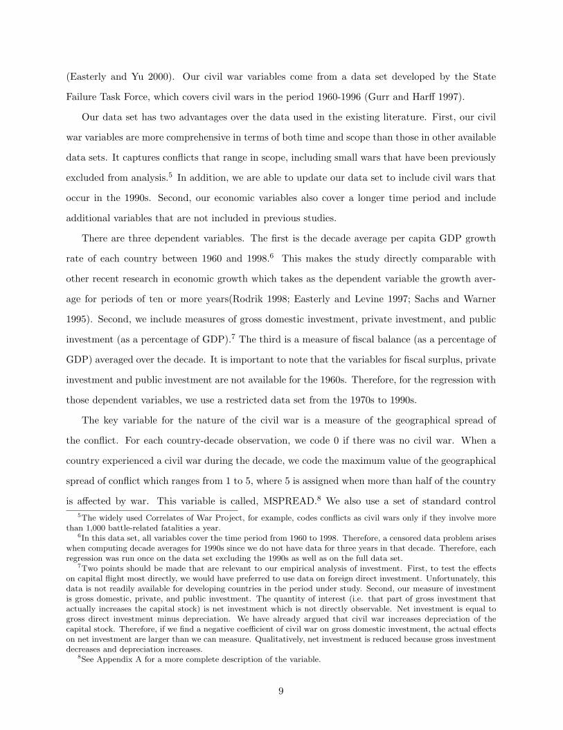
There are three dependent variables. The first is the decade average per capita GDP growth

rate of each country between 1960 and 1998.6 This makes the study directly comparable with

other recent research in economic growth which takes as the dependent variable the growth aver-

age for periods of ten or more years(Rodrik 1998; Easterly and Levine 1997; Sachs and Warner

1995). Second, we include measures of gross domestic investment, private investment, and public

investment (as a percentage of GDP).7 The third is a measure of fiscal balance (as a percentage of

GDP) averaged over the decade. It is important to note that the variables for fiscal surplus, private

investment and public investment are not available for the 1960s. Therefore, for the regression with

those dependent variables, we use a restricted data set from the 1970s to 1990s.

The key variable for the nature of the civil war is a measure of the geographical spread of

the conflict. For each country-decade observation, we code 0 if there was no civil war. When a

country experienced a civil war during the decade, we code the maximum value of the geographical

spread of conflict which ranges from 1 to 5, where 5 is assigned when more than half of the country

is affected by war. This variable is called, MSPREAD.8 We also use a set of standard control5The widely used Correlates of War Project, for example, codes conflicts as civil wars only if they involve more

than 1,000 battle-related fatalities a year.6In this data set, all variables cover the time period from 1960 to 1998. Therefore, a censored data problem arises

when computing decade averages for 1990s since we do not have data for three years in that decade. Therefore, eachregression was run once on the data set excluding the 1990s as well as on the full data set.

7Two points should be made that are relevant to our empirical analysis of investment. First, to test the effectson capital flight most directly, we would have preferred to use data on foreign direct investment. Unfortunately, thisdata is not readily available for developing countries in the period under study. Second, our measure of investmentis gross domestic, private, and public investment. The quantity of interest (i.e. that part of gross investment thatactually increases the capital stock) is net investment which is not directly observable. Net investment is equal togross direct investment minus depreciation. We have already argued that civil war increases depreciation of thecapital stock. Therefore, if we find a negative coefficient of civil war on gross domestic investment, the actual effectson net investment are larger than we can measure. Qualitatively, net investment is reduced because gross investmentdecreases and depreciation increases.

8See Appendix A for a more complete description of the variable.

9

variables in our regressions. We include dummy variables for each decade and continent dummies,

to control for decade and regional fixed effects. In addition, we include two variables measuring

national endowments at the start of the decade: the level of secondary schooling and the level

of per capita income. Following the standard growth model specification, we take a log for the

schooling variable and square the initial income level. Other macroeconomic control variables are

the black market premium (BMP) and inflation rate (INFLAT).

Finally, we introduce three country-specific effects. First, the level of ethno-linguistic fraction-

alization (ETHNIC), which has been used previously in a series of growth studies (Rodrik 1998;

Rodrik 1999; Easterly and Levine 1997). Second, we control for whether the country is land-locked

(LANDLOCK). Being land-locked is an exogenous impediment to trade and growth (Sachs and

Warner 1995). Third, we include a dummy variable capturing whether the country is a major oil

exporter (OILEXP).9 All these variables are taken from the Global Development Network Growth

Database.

4.2 Result 1: Growth effect

In our first specification, we run pooled ordinary least squares regressions. The growth performance

in each decade is treated as an independent observation ignoring the fact that the same country

may appear three times. This is a common model used in existing studies of this topic (Easterly

and Levine 1997; Collier 1999). Table 1 presents the results of the regression using the full data

set from the 1960s to the 1990s.

The results give strong support to our Growth and Geographical Spread Hypotheses. As a civil

war spreads widely throughout a country, the negative effect of war on the economic growth rate

increases. Further, this result is consistent with the study by Collier. The size of the coefficient

indicates that as the level of geographical spread of conflict increases by one unit, the decade-

average annual growth rate per capita decreases by about 0.2 percent. However, a reservation

needs to be made about the robustness of this result. The growth equation is somewhat sensitive

to minor changes of the model specification. For example, when we ran the separate regression

excluding the observations of 1990s, the statistical significance of the coefficient for MSPREAD9If a country is an oil exporter, we would expect a high fiscal surplus as well as high growth rates, holding

everything else constant.

10

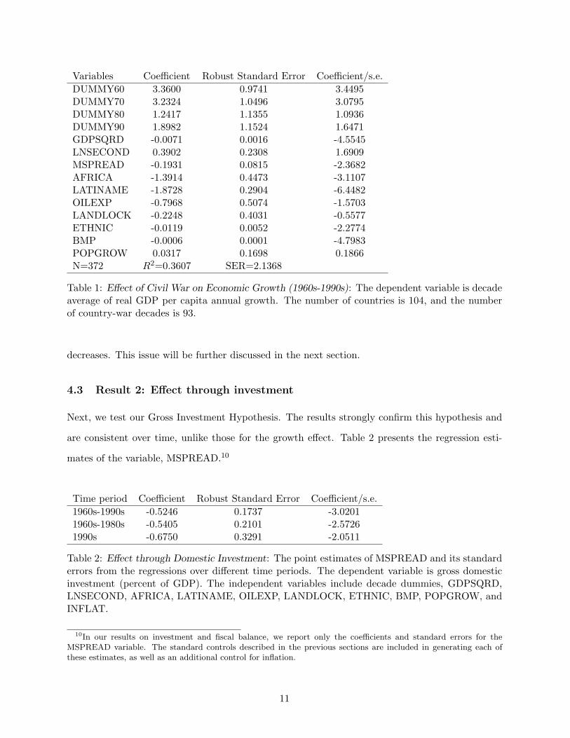
Variables Coefficient Robust Standard Error Coefficient/s.e.DUMMY60 3.3600 0.9741 3.4495DUMMY70 3.2324 1.0496 3.0795DUMMY80 1.2417 1.1355 1.0936DUMMY90 1.8982 1.1524 1.6471GDPSQRD -0.0071 0.0016 -4.5545LNSECOND 0.3902 0.2308 1.6909MSPREAD -0.1931 0.0815 -2.3682AFRICA -1.3914 0.4473 -3.1107LATINAME -1.8728 0.2904 -6.4482OILEXP -0.7968 0.5074 -1.5703LANDLOCK -0.2248 0.4031 -0.5577ETHNIC -0.0119 0.0052 -2.2774BMP -0.0006 0.0001 -4.7983POPGROW 0.0317 0.1698 0.1866N=372 R2=0.3607 SER=2.1368

Table 1: Effect of Civil War on Economic Growth (1960s-1990s): The dependent variable is decadeaverage of real GDP per capita annual growth. The number of countries is 104, and the numberof country-war decades is 93.

decreases. This issue will be further discussed in the next section.

4.3 Result 2: Effect through investment

Next, we test our Gross Investment Hypothesis. The results strongly confirm this hypothesis and

are consistent over time, unlike those for the growth effect. Table 2 presents the regression esti-

mates of the variable, MSPREAD.10

Time period Coefficient Robust Standard Error Coefficient/s.e.1960s-1990s -0.5246 0.1737 -3.02011960s-1980s -0.5405 0.2101 -2.57261990s -0.6750 0.3291 -2.0511

Table 2: Effect through Domestic Investment: The point estimates of MSPREAD and its standarderrors from the regressions over different time periods. The dependent variable is gross domesticinvestment (percent of GDP). The independent variables include decade dummies, GDPSQRD,LNSECOND, AFRICA, LATINAME, OILEXP, LANDLOCK, ETHNIC, BMP, POPGROW, andINFLAT.

10In our results on investment and fiscal balance, we report only the coefficients and standard errors for theMSPREAD variable. The standard controls described in the previous sections are included in generating each ofthese estimates, as well as an additional control for inflation.

11

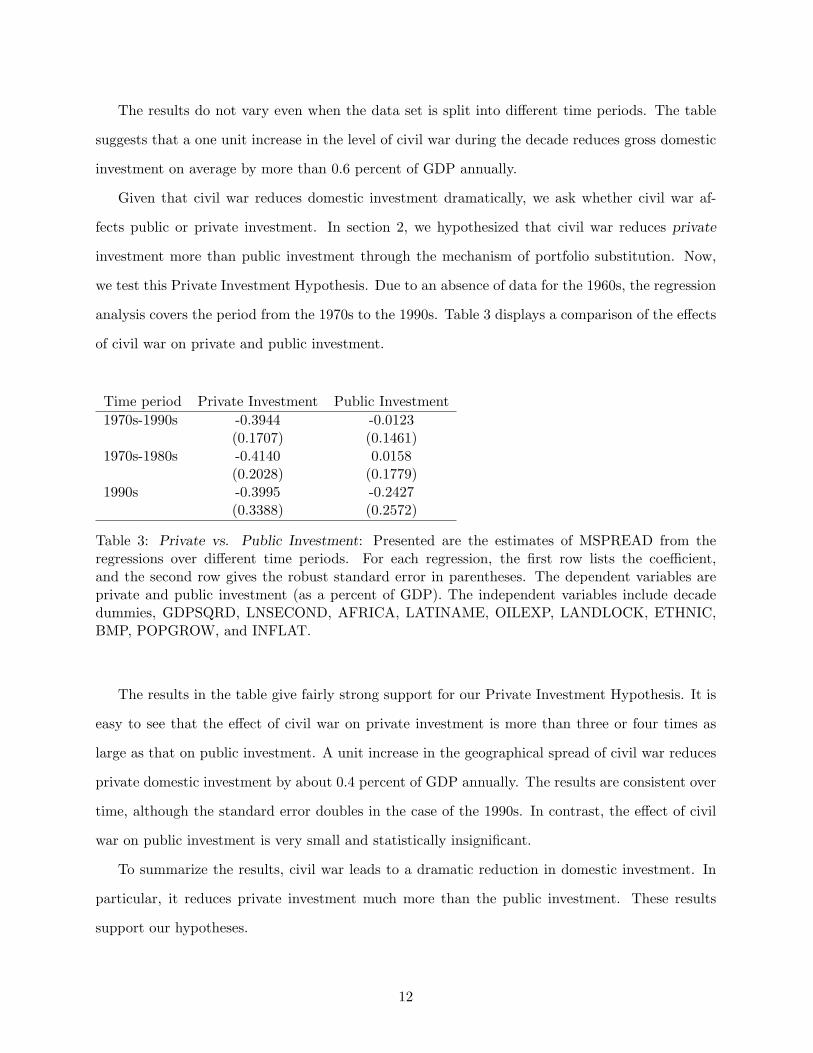
The results do not vary even when the data set is split into different time periods. The table

suggests that a one unit increase in the level of civil war during the decade reduces gross domestic

investment on average by more than 0.6 percent of GDP annually.

Given that civil war reduces domestic investment dramatically, we ask whether civil war af-

fects public or private investment. In section 2, we hypothesized that civil war reduces private

investment more than public investment through the mechanism of portfolio substitution. Now,

we test this Private Investment Hypothesis. Due to an absence of data for the 1960s, the regression

analysis covers the period from the 1970s to the 1990s. Table 3 displays a comparison of the effects

of civil war on private and public investment.

Time period Private Investment Public Investment1970s-1990s -0.3944 -0.0123

(0.1707) (0.1461)1970s-1980s -0.4140 0.0158

(0.2028) (0.1779)1990s -0.3995 -0.2427

(0.3388) (0.2572)

Table 3: Private vs. Public Investment: Presented are the estimates of MSPREAD from theregressions over different time periods. For each regression, the first row lists the coefficient,and the second row gives the robust standard error in parentheses. The dependent variables areprivate and public investment (as a percent of GDP). The independent variables include decadedummies, GDPSQRD, LNSECOND, AFRICA, LATINAME, OILEXP, LANDLOCK, ETHNIC,BMP, POPGROW, and INFLAT.

The results in the table give fairly strong support for our Private Investment Hypothesis. It is

easy to see that the effect of civil war on private investment is more than three or four times as

large as that on public investment. A unit increase in the geographical spread of civil war reduces

private domestic investment by about 0.4 percent of GDP annually. The results are consistent over

time, although the standard error doubles in the case of the 1990s. In contrast, the effect of civil

war on public investment is very small and statistically insignificant.

To summarize the results, civil war leads to a dramatic reduction in domestic investment. In

particular, it reduces private investment much more than the public investment. These results

support our hypotheses.

12

4.4 Result 3: Effect through fiscal policy

An alternative explanation is that civil war impacts economic growth through its effect on fiscal

policy. Our Fiscal Policy Hypothesis states that civil war negatively affects the domestic economy

by increasing the government budget deficit. The results of our analysis are summarized in Table 4.

Time period Coefficient Robust Standard Error Coefficient/s.e.1970s-1990s -0.0037 0.1187 -0.03151970s-1980s -0.0184 0.1567 -0.11731990s 0.0653 0.1735 0.3762

Table 4: Effect through Fiscal Deficit: Presented are the estimates of MSPREAD from the regres-sions over different time periods. The dependent variable is overall Budget Surplus (percent ofGDP). The independent variables are private and public investment (percent of GDP).

Our results suggest that civil war has almost no effect on the level of fiscal balance. In contrast

with its effect on domestic investment, the size of coefficient for MSPREAD is very small. Further,

these results are consistent over time.

In summary, our OLS regressions demonstrate three points. First, the results show that the

more geographically spread the conflict, the larger its negative impact on economic growth. Sec-

ond, and most importantly, the driving force behind the negative effect of civil war on the domestic

economy is a dramatic reduction in domestic investment. In particular, we find that private in-

vestment rather than public investment is reduced during internal conflict. This evidence supports

the theory that civil war causes dramatic decreases in domestic investment through capital flight

and portfolio substitution, leading to a decrease in the growth rate of GDP. Finally, there is little

connection between civil war and fiscal balance. Political economy models suggest that civil war

leads to an increase in budget deficit. Our analysis finds no evidence for such an argument.

5 Improving Estimation

In this section, we use more sophisticated methods to improve our statistical analysis and test the

robustness of our findings. We address the missing data problem by utilizing multiple imputation

methods to simulate missing values using all the information available in our data set. Second, we

improve the model by exploiting the panel characteristics of the data set. The straight application

13

of a pooled OLS model to panel data can introduce bias and consequently lead to false substantive

conclusions. Despite a large body of literature on this topic, researchers often use OLS models for

the analysis of panel data. We hope to fill this gap between the previous empirical research and

existing statistical methodology.

5.1 Multiple imputation method

A significant problem in the analysis of conflict and growth is missing data. World Bank and IMF

data sets rarely have complete information on lesser developed countries. Our data is no exception

to this problem. For example, the full data set includes observations for four decades and 212

countries (a total of 848 observations). With complete information about civil war, we know that

142 country-decades are characterized by civil war. Using list-wise deletion, which is standard

practice in the literature, requires us to reduce the data set to 372 observations, of which 93 are

civil war country-decades. As a result, the data set on which we conduct our preliminary analysis

has a rate of civil war occurrence approaching 25 percent, while the true population percentage is

closer to 16 percent. It is highly probable that this over-representation of war country-decades in

the reduced sample leads to inaccurate estimation.

A multiple imputation technique enables us to improve estimation of the economic effects of

conflict. We utilize all available information about the full sample of countries to generate imputed

values of the data where it is missing. Following King et al. (2000), we impute five values for

each missing data point and create five complete data sets. Across these completed data sets, the

observed values are the same, but the missing values are filled in with different imputations to

reflect uncertainty levels. For missing cells that the model can predict well, the variation across

data sets is small. In other cases, the variation may be much larger. A more detailed description

of the procedure is available in Appendix C. Next, we introduce the panel data models which will

be applied to these imputed data sets.

5.2 Models for panel data

Recently, there has been an expanding empirical literature on economic growth.11 In the neo-

classical economic growth model, a country’s GDP is a Cobb-Douglas production function with11See Barro and Sala-i-Martin (1999) for an extensive literature review.

14

respect to structural variables such as labor force, physical capital and technology. An implication

of this model is that if countries are similar to each other in those structural variables, then poor

countries grow faster than rich countries. Hence, Barro (1991) and Mankiw et al. (1992) find that

while there is no correlation between the level of a country’s income and its subsequent growth rate,

when controlling for human capital as well as the structural variales, there is a strong evidence to

suggest that there exists a force of convergence.

However, these studies along with the literature on political conflicts and economic growth

(Easterly and Levine 1997; Collier 1999), use pooled ordinary least squares. This is based on the

assumption that the aggregate production function is identical across countries. However, such

an assumption is unlikely to hold given the different characteristics of each country in the world.

The panel data approach allows one to take into consideration unobservable differences in the

production function specific to individual countries. The result of the violation of this assumption

is omitted variable bias which is likely to bias all the coefficients in a regression.

For a panel data which has a short time series and many countries, the error-components model

has proven to be useful in overcoming the potential bias introduced by pooled OLS. Moreover, such

an approach has already been used to analyze panel data on economic growth (Islam 1995). This

paper follows these studies in using panel data approaches to analyze the impact of civil war on

economic growth.

We use two basic error-components models: fixed and random effects estimation. The fixed

effects estimation is the most intuitive way to control for unobservable effects specific to individual

countries in panel data. The key assumptions of this model are that country specific effects do not

vary over time and that they are correlated with other regressors. In the present context, this model

allows one to control for country specific characteristics of the production function which do not

vary over time. As a consequence, the fixed effects estimation should not include country-specific

variables.12

The second model is random effects estimation. Compared with fixed effects estimation, this

model achieves more efficient estimation at the risk of reducing consistency. Specifically, the random12Although this point seems trivial, some researchers mistakenly include country-specific variables. For example,

Collier (1999) includes a dummy variable for being landlocked and a variable of ethnic fractionalization both of whichdo not vary over time for each country. This leads to a significant bias in his results despite his claim that OLSshould be preferred over the fixed effects estimation.

15

effects estimation makes an additional assumption that country specific effects are uncorrelated with

other regressors. If this assumption is satisfied, researchers can exploit additional orthogonality

conditions to obtain more efficient estimators without the loss of consistency. The choice of one

model over the other is the tradeoff between consistency and efficiency. We use the Hausman

specification test to determine which of the two models is appropriate for our analysis.13

5.3 Results

The Hausman specification test supports random effects estimation for all five regressions. For

example, the Hausman statistic for the growth regression is 8.1482 with 8 degrees of freedom,

failing to reject the maintained hypothesis that error term is uncorrelated with regressors. This

implies that by using random effects estimation, we can obtain more efficient estimators without

sacrificing consistency.

Table 5 presents the random effects estimation of the impact of civil war on the growth rate

of GDP. These results lend additional support to our growth hypothesis. The coefficient on

MSPREAD in the regression increases in magnitude and becomes more statistically significant

when we control for unobservable differences in the countries included. As compared to the pooled

OLS regression, the coefficient on MSPREAD increases from -0.19 to -0.26, with the t-statistic

increasing from -2.37 to -3.09. Substantively, this result suggests that a geographically spread

conflict reduces the annual growth rate by 1.25 percent. Since panel data models enable us to

control for all unobserved country-specific differences, we can be sure that this approach yields a

more accurate and consistent estimate of the economic effects of war. Moreover, by including all

available data and imputing missing values, we reduce estimation bias that may come from listwise

deletion.

Given the strong negative impact of civil war on economic growth, we move on to test our main

arguments on the channels through which civil war affects economic growth. Table 6 presents the

results. Our Domestic Investment hypothesis obtains strong support. An internal conflict spread13The Hausman statistic is defined as H ≡ q̂′( \Avar(q̂))−1q̂ where q̂ ≡ β̂FE − β̂RE and Avar(q̂) ≡ Avar(β̂FE) −

Avar(β̂RE). Avar(•) represents asymptotic variance of an estimator and β̂FE , β̂RE denote estimators of fixed andrandom effects estimation, respectively. In order to calculate one total variance covariance matrix from five imputeddata sets, we use the formula following Schafer(1997, chapter 3).

16

Variables Coefficient Robust Standard Error Coefficient/s.e.GDPSQRD -0.0046 0.0009 -4.877LNSECOND 0.4631 0.0931 4.9757MSPREAD -0.2644 0.0857 -3.0858BMP -0.0002 0.0000 -6.1372POPGROW -0.1694 0.0846 -2.0025AFRICA -0.1758 0.2569 -0.6844LATINAME -0.5035 0.4671 -1.0777ETHNIC -0.0046 0.0098 -0.4700OILEXP 0.1920 0.2980 0.6443LANDLOCK -0.7171 0.5277 -1.3589

Table 5: Random Effects Estimation of Impacts of Civil War on Economic Growth (1960s to 1990s):Results are based on five regressions on imputed data sets. Decade dummies are omitted from thetable.

throughout the country decreases domestic investment by more than 4 percent. The impact of the

civil war variable, MSPREAD, on domestic investment is actually much larger than estimated in

the OLS regression (see table 2), while the standard error remains at the same level. This suggests

that the estimation of OLS was biased downward, underestimating the negative effects of civil war

on domestic investment.

Dependent Variables Coefficients Robust Standard Errors tratioDomestic Investment -0.8202 0.1684 -4.8710Surplus -0.0894 0.0952 -0.9389Private Investment -0.5290 0.1779 -2.9734Public Investment -0.1625 0.1256 -1.2931

Table 6: Random Effects Estimation of Economic Impacts of Civil War (Estimators forMSPREAD): Results are based on five regressions on imputed data sets. The original regres-sions include the same control variables as in the growth regression of table 5 as well as an inflationvariable. The time period for domestic investment runs from the 1960s to the 1990s, whereas theother three variables cover from the 1970s to the 1990s.

Our evidence using random effects also enables us to reject the fiscal balance hypothesis. The

coefficient is very small indicating that the effects of civil war on a government’s fiscal balance are

almost nonexistent. Finally, the evidence gives strong support to our conjecture that the most

destructive effect of civil war is through reduction in private rather than public investment. Again,

the comparison with the result of the pooled OLS model is instructive. It is clear that the OLS

17

results (see table 3) underestimate the effect of civil war on private investment as in the result for

domestic investment.

In this section, we make two methodological improvements. First, we fill in missing values in

our data set by using a multiple imputation technique. Second, we use random effects estimation

to correct omitted variable bias produced by the pooled OLS estimation. The evidence strongly

supports our theory that civil war negatively affects the domestic economy by reducing private

investment. Moreover, the random effects estimation corrects the bias introduced by pooled OLS

estimation which underestimates the effects of civil war on growth and investment.

6 Reinterpretation of the Model Prediction

Our paper so far has shown that civil war negatively affects the domestic economy by reducing

domestic investment. However, we also see that the growth equation is very sensitive to minor

changes of its specification. We show in this section that this is due to fundamental uncertainty

that the standard growth model fails to capture. Economic models are often associated with high

degree of noise. Hence, even when the estimation uncertainty is very small, it is possible that the

model suffers from a large fundamental uncertainty. Ignoring this results in the overestimation of

the accuracy of the model’s predictions.

We illustrate the problem of ignoring the fundamental uncertainty by using the method sug-

gested by King et al. (2000). We simulate fitted values by taking into account the fundamental as

well as the estimation uncertainty. While the standard error of the coefficient reflects the uncer-

tainty around the corresponding point estimate, the fundamental uncertainty of the model is left

unexplained. Let us go back to our growth regression shown in Table 1. The table shows that the

coefficient of MSPREAD is significant with a relatively small standard error. However, the small

value of R2 indicates that a large part of the variance is not explained by the model. This suggests

that the fundamental uncertainty associated with the model is substantially large.

We explore the implications of this problem by simulating the expected growth rate and its 95

percent confidence interval for a particular type of country.14 Table 7 shows the growth effect of14In order to use this simulation technique, we reestimated the growth regression under the additional assumption

that the error term is normally distributed. Hence, our reestimation utilizes a linear normal probability model ofmaximum likelihood estimation rather than OLS. Note that the point estimates of the two models are identical,though standard errors are slightly different.

18

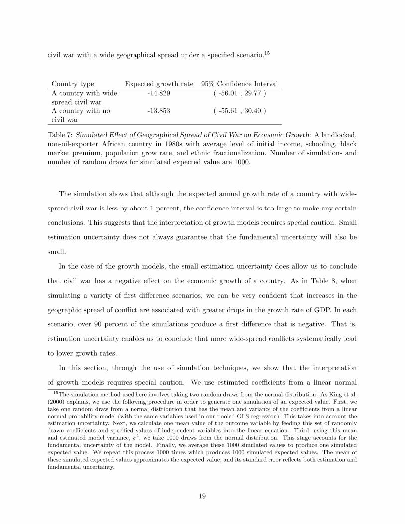
civil war with a wide geographical spread under a specified scenario.15

Country type Expected growth rate 95% Confidence IntervalA country with wide -14.829 ( -56.01 , 29.77 )spread civil warA country with no -13.853 ( -55.61 , 30.40 )civil war

Table 7: Simulated Effect of Geographical Spread of Civil War on Economic Growth: A landlocked,non-oil-exporter African country in 1980s with average level of initial income, schooling, blackmarket premium, population grow rate, and ethnic fractionalization. Number of simulations andnumber of random draws for simulated expected value are 1000.

The simulation shows that although the expected annual growth rate of a country with wide-

spread civil war is less by about 1 percent, the confidence interval is too large to make any certain

conclusions. This suggests that the interpretation of growth models requires special caution. Small

estimation uncertainty does not always guarantee that the fundamental uncertainty will also be

small.

In the case of the growth models, the small estimation uncertainty does allow us to conclude

that civil war has a negative effect on the economic growth of a country. As in Table 8, when

simulating a variety of first difference scenarios, we can be very confident that increases in the

geographic spread of conflict are associated with greater drops in the growth rate of GDP. In each

scenario, over 90 percent of the simulations produce a first difference that is negative. That is,

estimation uncertainty enables us to conclude that more wide-spread conflicts systematically lead

to lower growth rates.

In this section, through the use of simulation techniques, we show that the interpretation

of growth models requires special caution. We use estimated coefficients from a linear normal15The simulation method used here involves taking two random draws from the normal distribution. As King et al.

(2000) explains, we use the following procedure in order to generate one simulation of an expected value. First, wetake one random draw from a normal distribution that has the mean and variance of the coefficients from a linearnormal probability model (with the same variables used in our pooled OLS regression). This takes into account theestimation uncertainty. Next, we calculate one mean value of the outcome variable by feeding this set of randomlydrawn coefficients and specified values of independent variables into the linear equation. Third, using this meanand estimated model variance, σ2, we take 1000 draws from the normal distribution. This stage accounts for thefundamental uncertainty of the model. Finally, we average these 1000 simulated values to produce one simulatedexpected value. We repeat this process 1000 times which produces 1000 simulated expected values. The mean ofthese simulated expected values approximates the expected value, and its standard error reflects both estimation andfundamental uncertainty.

19

MSPREAD Estimated 95% negativeScenario (from, to) first diff. confidence interval first diff.no war to minor war (0,1) 0.1900 (-0.0504, 0.4101) 94.0 %minor to medium war (1,3) 0.3880 (0.0246, 0.7130) 98.2no war to major war (0,5) 0.9454 (0.1902, 1.690) 99.2

Table 8: Simulated First Differences for Effect of Geographical Spread of Civil War on EconomicGrowth: Changing the values of MSPREAD while holding the other variables at their means. Thenumbers of simulations and number of random draws for simulated expected value are 1000.

probability model that mirrors our pooled OLS regression, but the substantive conclusions hold

equally well for the fundamental uncertainty represented in our fixed and random effects models.

A small degree of uncertainty around our point estimates of marginal effects enables us to make

important conclusions about the marginal impact of increases in the geographic spread of conflict

on growth. However, making predictions about the actual effects of war on growth based on such

poorly-fit models is risky. When we take into account the fundamental uncertainty associated with

models of growth, we are unable to draw clear conclusions.

7 Conclusion

In this paper, we have four main findings. First, civil war has a negative impact on economic

growth. The rate of growth of the capital stock is reduced as civil war drives down domestic

investment. In particular, civil wars reduce private investment because private agents are better

able to respond to increases in the uncertainty of the economic environment. We find no evidence

that civil wars have negative effects on the fiscal balance of governments.

Second, we find that the effect on growth depends on the scope of civil war. By assuming away

variation across civil wars, the estimate of economic effects is imprecise. We improve existing studies

by introducing a measurement of civil war variation that reflects differences in the geographic spread

of war. The results suggest that wide-spread civil wars are five times more costly than narrowly

fought internal conflicts and reduce GDP growth rates by 1.25 percent a year.

Third, we improve estimation by imputing missing data and applying more appropriate statis-

tical models to the analysis of political influences on economic outcomes. We argue that the use

of pooled OLS models may result in incorrect substantive conclusions when unobservable cross-

20

country differences are not taken into account. Fixed and random effects models lend support to

our arguments about the links between civil war and the economy, and more accurately fit the

structure of the data used in this and previous analyses.

Finally, we qualify our results by systematically exploring the uncertainty associated with the

point estimates of economic cost. In doing so, we recognize problems of fundamental uncertainty

that the previous literature ignores. Although the point estimates of the civil war variables are

statistically significant often at the 99 percent level, the model specification of economic growth is

poor. As a result, the economic effects of conflict disappear when we run simulations to compute the

expected effects for different scenarios. The expected effects, even across thousands of simulations,

have large variance and fail to support clear cut conclusions about the costs of conflict.

21

A Data description

Code Book for Civil War Data Set, 1960-1996Kosuke Imai, and Jeremy Weinstein

Identification VariablesCCODE Three-letter country code.COUNTRY Country name.DECADE Period of 10 years over which variables are averaged. Can take the value of

60,70,80,90.

Macroeconomic Variables (1960-1998)GROWTH Real GDP per capita growthBMP Black market premium (%)SURPLUS Budget surplus excluding capital grants (% of GDP)DOMINV Gross domestic investment (% of GDP)PUBINV Public investment (% of GDP)PRIINV Private investment (% of GDP)GDPSQRD (Real GDP per capita at the beginning of decade/1000)^2POPGROW Population growth (%)INFLAT Inflation rate (%)

Social Indicators (1960-1998)LNSECOND ln (Secondary School enrollment(% gross))

Control VariablesLANDLOCK Dummy variable for landlocked.OILEXP Dummy variable for oil exporter.ETHNIC Index of ethnic fractionalization. The probability of two randomly

drawn people from the population being from different ethno-linguisticgroups.

AFRICA Dummy variable for Sub-Saharan Africa.LATINAME Dummy variable for Latin America.DUMMY60 Decade dummy variable for 1960s.DUMMY70 Decade dummy variable for 1970s.DUMMY80 Decade dummy variable for 1980s.DUMMY90 Decade dummy variable for 1990s.

Source:Global Development Network Growth Database. William Easterly and Hairong Yu. Datacan be obtained at http://www.worldbank.org/growth/GDNdata.htm#4.

Civil War VariableOur sample of civil wars is drawn from the State Failure Task Force data set. We include both

revolutionary and ethnic wars in our sample. Definitions of each from the State Failure Task Forceare included below.

22

Revolutionary wars are episodes of violent conflict between governments and politically orga-nized groups (political challengers) that seek to overthrow the central government, to replace itsleaders, or to seize power in one region. Conflicts must include substantial use of violence by oneor both parties to qualify as ”wars.”

”Politically organized groups” may include revolutionary and reform movements, political par-ties, student and labor organizations, and elements of the armed forces and the regime itself. Ifthe challenging group represents a national, ethnic, or other communal minority, the conflict isanalyzed as an Ethnic war, below.

¿From the 1950s through the late 1980s most revolutionary wars were fought by guerrilla armiesorganized by clandestine political movements. Some wars, usually smaller in scale, relied wholly orin part on campaigns of terrorism. A few, like the Iranian revolution of 1979, were mass movementsthat organized campaigns of demonstrations. The violence and fatalities in revolutionary conflictsof this type were mainly the result of government repression. The student revolutionary movementin China that was suppressed in the Tiananmen Square massacre in 1989 is another example. Mostmass movements that precipitated the fall of East European communist governments in 1989-90do NOT qualify as revolutionary wars because neither party used substantial violence.

These are the minimum thresholds for including a revolutionary conflict in the updated statefailure dataset: each party must mobilize 1000 or more people (armed agents, demonstrators,troops) and an average of 100 or more fatalities per year must occur during the episode.

Ethnic wars are episodes of violent conflict between governments and national, ethnic, religious,or other communal minorities (ethnic challengers) in which the challengers seek major changes intheir status. Most ethnic wars since 1955 have been guerrilla or civil wars in which the challengershave sought independence or regional autonomy. A few, like the events in South Africa’s blacktownships in 1976-77, involved large-scale demonstrations and riots aimed at sweeping politicalreform that were violently suppressed by police and military. Rioting and warfare between rivalcommunal groups is NOT coded as ethnic warfare unless it involves conflict over political power orgovernment policy.

As with revolutionary wars, the minimum thresholds for including an ethnic conflict in theupdated state failure data set are that each party must mobilize 1000 or more people (armedagents, demonstrators, troops) and an average of 100 or more fatalities per year must occur duringthe episode. The fatalities may result from armed conflict, terrorism, rioting, or governmentrepression.

The original Variable: MAGAREA.Portion of country affected by fighting. Code based on source materials abouthow much of the country is directly or indirectly affected by fighting orrevolutionary protest in a given year. A province, region, or city is "directlyaffected" if fighting/terrorist attacks/revolutionary protest occur there atany time during the year. It is "indirectly affected" if the area has significantspillover effects from nearby fighting, for example refugees flows, curtailmentof public services, martial law imposed. If open conflict expands or contractsduring the course of the year, code according to its greatest extent.

0 = less than one-tenth of the country and no significantcities are directly or indirectly affected

1 = one-tenth of the country (one province or state) and/orone or several provincial cities are directly orindirectly affected

23

2 = more than one-tenth and up to one quarter of the country(several provinces or states) and/or the capital city aredirectly or indirectly affected

3 = from one-quarter to one-half the country and/or most majorurban areas are directly or indirectly affected

4 = more than one-half the country is directly or indirectlyaffected

MSPREAD The maximum value of MAGAREA in a decade for each country.

Source:State Failure Task Force Data Set. Available to the public athttp://www.bsos.umd.edu/cidcm/stfail/.

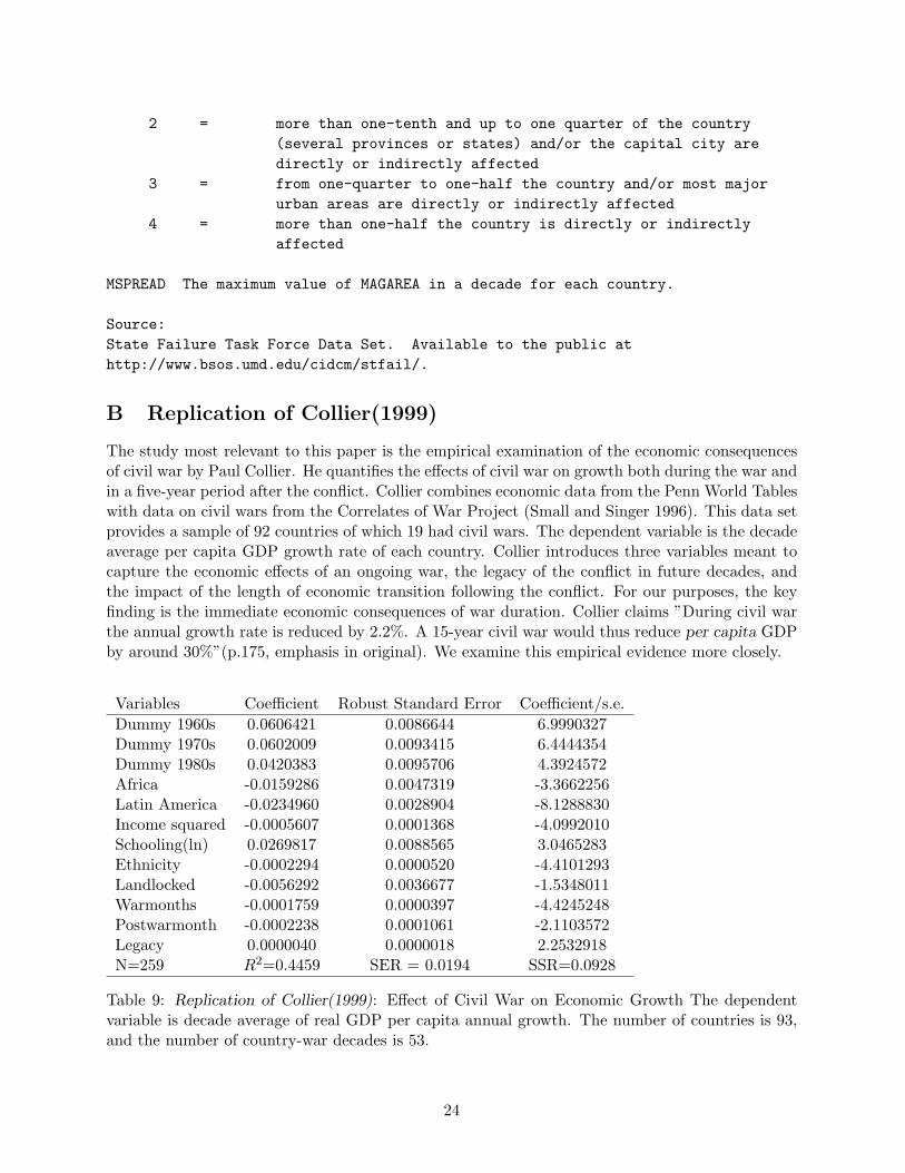
B Replication of Collier(1999)

The study most relevant to this paper is the empirical examination of the economic consequencesof civil war by Paul Collier. He quantifies the effects of civil war on growth both during the war andin a five-year period after the conflict. Collier combines economic data from the Penn World Tableswith data on civil wars from the Correlates of War Project (Small and Singer 1996). This data setprovides a sample of 92 countries of which 19 had civil wars. The dependent variable is the decadeaverage per capita GDP growth rate of each country. Collier introduces three variables meant tocapture the economic effects of an ongoing war, the legacy of the conflict in future decades, andthe impact of the length of economic transition following the conflict. For our purposes, the keyfinding is the immediate economic consequences of war duration. Collier claims ”During civil warthe annual growth rate is reduced by 2.2%. A 15-year civil war would thus reduce per capita GDPby around 30%”(p.175, emphasis in original). We examine this empirical evidence more closely.

Variables Coefficient Robust Standard Error Coefficient/s.e.Dummy 1960s 0.0606421 0.0086644 6.9990327Dummy 1970s 0.0602009 0.0093415 6.4444354Dummy 1980s 0.0420383 0.0095706 4.3924572Africa -0.0159286 0.0047319 -3.3662256Latin America -0.0234960 0.0028904 -8.1288830Income squared -0.0005607 0.0001368 -4.0992010Schooling(ln) 0.0269817 0.0088565 3.0465283Ethnicity -0.0002294 0.0000520 -4.4101293Landlocked -0.0056292 0.0036677 -1.5348011Warmonths -0.0001759 0.0000397 -4.4245248Postwarmonth -0.0002238 0.0001061 -2.1103572Legacy 0.0000040 0.0000018 2.2532918N=259 R2=0.4459 SER = 0.0194 SSR=0.0928

Table 9: Replication of Collier(1999): Effect of Civil War on Economic Growth The dependentvariable is decade average of real GDP per capita annual growth. The number of countries is 93,and the number of country-war decades is 53.

24

Table 8 shows our replication of his result.16 Warmonths is the months of warfare duringthe decade, and Postwarmonths is the number of potential recovery months during the decade.The final variable, Legacy, interacts Warmonths with Postwarmonths and is meant to capture theconcurrent effects of war on growth. The two additional variables focus on the economic impact ofconflict in the first five post-war years.

Although we could successfully replicate Collier’s analysis, we offer a slightly different inter-pretation of the result. For now, we briefly point out that the −2.2% annual growth rate thatCollier gives as result from a year-long war is actually the result for the effect of a decade-long war.Furthermore, the effect of a 15-year civil war is −3.4% rather than −30% as he claims. Hence,although civil war has a negative impact on economic growth, the size of the impact seems muchsmaller than what Collier reported.

C Note on multiple imputation procedure

Using the multiple imputation program developed by King et al. (2000), we impute a set of fivedata sets for each of the two time periods: one from the 1960s to 1990s and the other from the1970s to 1990s. This is done because three of our five dependent variables (SURPLUS, PRIINV,and PUBINV) do not have any observations for the 1960s.

For the data set which runs from the 1960s to 1990s, the following variables are included whenimputing the missing observations.

GROWTH LNGDPST LNDOMINV BMP INFLAT POPGROW LNSECOND AFRICA LATI-NAME LANDLOCK OILEXP HIGHOECD LNETHNIC MSPREAD

We take log for the initial level of GDP and ETHNIC since these are proportions and needto be transformed to be close to the normal distributions. We take one decade lag of the first 7variables. Each of the resulting five data sets has 848 observations.

For the data set from the 1970s to 1990s, we also impute investment and surplus variables.

GROWTH LNGDPST BMP SURPLUS LNPRIINV LNPUBINV INFLAT POPGROW LNSEC-OND AFRICA LATINAME LANDLOCK OILEXP HIGHOECD LNETHNIC MSPREAD

Again, as in the first data set, we take one-decade lag of the first 9 variables to impute fivedata sets each of which has 636 observations.

16The value of R2 is slightly different since he uses adjusted R2, whereas we use a non-adjusted one.

25

References

Alesina, Alberto and G. Tabellini. 1990. “A Positive Theory of Fiscal Deficits and GovernmentDebt.” Review of Economic Studies 57 (3): 403–414.

Barro, Robert J. 1991. “Economic Growth in a Cross Section of Countries.” Quarterly Journalof Economics 106 (2): 407–443.

Barro, Robert J. and Xavier Sala i Martin. 1999. Economic Growth. Cambridge, Mass: MITPress.

Collier, Paul. 1999. “On the Economic Consequences of Civil War.” Oxford Economic Paper 51(1): 168–183.

Easterly, William and Ross Levine. 1997. “Africa’s Growth Tragedy: Policies and Ethnic Divi-sions.” Quarterly Journal of Economics 112 (4): 1203–1250.

Easterly, William and H. Yu. 2000. “Global Development Growth Network Database.” TechnicalReport, World Bank.

Edwards, Sebastian and Guido Tabellini. 1991. “Explaining Fiscal Policies and Inflation inDeveloping Countries.” Journal of International Money and Finance, vol. 10.

Fischer, Stanley. 1993. “The Role of Macroeconomic Factors in Growth.” Journal of MonetaryEconomics 32 (3): 485–512.

Gurr, Ted and Barbara Harff. 1997. “Internal Wars and Failures of Governance, 1954-1996.”Technical Report, State Failure Task Force.

Islam, Nazrul. 1995. “Growth Empirics: A Panel Data Approach.” Quarterly Journal of Eco-nomics 110 (4): 1127–1170.

King, Gary, James Honaker, Anne Joseph, and Kenneth Scheve. 2000. “Analyzing IncompletePolitical Science Data: An Alternative Algorithm for Multiple Imputation.” UnpublishedManuscript. Harvard University.

King, Gary, Michael Tomz, and Jason Wittenberg. 2000. “Making the Most of Statistical Analysis:Improving Interpretation and Presentation.” American Journal of Political Science 44 (2):341–355.

Knight, Malcolm, Norman Loayza, and Delano Villanueva. 1996. “The Peace Dividend: MilitarySpending Cuts and Economic Growth.” IMF Staff Papers 43 (1): 1–37.

Mankiw, N. Gregory, David Romer, and David N. Weil. 1992. “A Contribution to the Empiricsof Economic Growth.” Quarterly Journal of Economics 107:407–437.

Rodrik, Dani. 1998. “The New Global Economy and Developing Countries: Making OpennessWork.” Report for Overseas Development Council.

. 1999. “Where Did All the Growth Go? External Shocks, Social Conflicts, and GrowthCollapses.” Journal of Economic Growth 4:385–412.

Roubini, Nouriel. 1991. “Economic and Political Determinants of Budget Deficits in DevelopingCountries.” Journal of International Money and Finance 10 (Supplement): S49–S72.

Sachs, Jeffrey and Andrew Warner. 1995. “Economic Reform and the Process of Global Integra-tion.” Brookings Papers in Economic Activity, no. 1:1–95.

Schafer, Joseph L. 1997. Analysis of Incomplete Multivariate Data. London: Chapman Hall.

26

Small, Melvin and J. David Singer. 1996. “Correlates of War Project: International and CivilWar Data: 1816-1992.” Technical Report, Inter-University Consortium for Political and SocialResearch.

27