1

Measuring the effectiveness of volatility

auctions Carlos Castro†1, Diego Agudelo‡, Sergio Preciado¶

† Universidad del Rosario, Bogotá, Colombia,

‡ Universidad EAFIT, Medellín, Colombia, and

¶ Infovalmer, Bogotá, Colombia

Abstract

We propose a method for event studies based on synthetic portfolios that provides a robust data-driven

approach to build a credible counterfactual. The method is used to evaluate the effectiveness of volatility

auctions using intraday data from the Colombian Stock Exchange. The results indicate that the synthetic

portfolio method provides an accurate way to build a credible counterfactual that approximates the

behavior of the asset if the auction had not taken place. The main results indicate that the volatility

auction mitigates the volatility of the asset, but its effect on liquidity and trading activity is ambiguous at

best.

Keywords: Circuit breakers, synthetic control, event studies, volatility auction, tracking portfolios

JEL Classification: C21, C58, G11, G14.

1 Corresponding author: Carlos Castro, carlos.castro@urosario.edu.co.

The authors thank participants at the XXIV Finance Forum in Madrid, Spain, the ICASQF 2016 conference in Cartagena, Colombia, seminar participants at Seminar Bachelier (Institut Louis Bachelier), Vlerick Business School, CESA Business School, Universidad del Rosario for helpful comments and suggestions concerning this research. The authors thank Bolsa de Valores de Colombia, in particular Adriana Cardenas and Ross MacDonald, for their interest and support in providing the auction data. We also thank Catalina Cadena, Juliana Hincapie, Julian Munera, and Paula Yepes for their excellent research assistance with the TAQ database of the assets traded on the BVC.

2

1. Introduction

Firm-specific trading halts are widely used in securities markets as a means of normalizing the trading

process in times of excessive volatility. They belong to the group of circuit breakers that also includes price

limits and market-wide trading halts (Kim and Yang 2004). Firm-specific trading halts are a common

feature of stock exchanges around the world, such as the NYSE, NASDAQ, and Euronext, and those of

Australia, Canada, Germany, Hong Kong, Israel, the UK, and Spain. However, there is no consensus on the

need for or the effectiveness of trading halts. Moreover, interest in trading halts and price limits have

rekindled in the aftermath of the Flash Crash in US futures and stock markets in May, 6, 2010 (Gomber,

Lutat, Haferkorn, and Zimmermann 2011; Subrahmanyam, 2013; Dalko, 2016) .

In principle, trading halts would be irrelevant in an efficient market because prices should respond

immediately to the arrival of new information. However, market microstructure considerations might

make them desirable. Specifically, trading halts have been justified as a way of mitigating the information

disadvantage of uninformed traders or designated market makers, enabling the market to better

accommodate large-volume shocks (Greenwald and Stein, 1988, 1991). Trading halts might also provide

a “cooling off” period that supposedly allows investors to better process the incoming information (Kim,

Yage and Yang, 2008). Theoretical models support this line of reasoning. Madhavan (1992), modeling a

continuous market versus call auctions, finds that “the periodic auction aggregates information efficiently

and is more robust to problems of information asymmetry in that it can operate where the continuous

market fails” (p. 609). Spiegel and Subrahmanyam (2002) offer a model in which trading halts signal large

information asymmetry affecting not only the halted stock, but also informationally related securities.

However, some academics oppose trading halts as undesired intrusions into a free market. Fama (1989)

is against the “cooling off” period, arguing that any investors who want to cool off can do so by simply

staying out of the market. Grossman (1990) states that investors, as “consenting adults”, should not be

prevented from trading as they please. Grundy and McNichols (1989) propose a model of “learning

through trading” that implies that in the absence of continuous trading potential traders are less able or

willing to reveal their demands and information. Moreover, the theoretical analysis of Subrahmanyam

(1994) finds that trading halts might have the perverse effect of exacerbating volatility because traders

might sub-optimally advance their trades in anticipation.

We study the effect on market quality of a particular type of trading halt on the Colombian Stock Exchange

(BVC): the rules-based volatility auction. As detailed below, volatility auctions on the BVC are trading halts

triggered by the imminence of a trade outside price collars, switching continuous trading to a short-lived

call auction. Like those of the Spanish Stock Exchange (SIBE) after May 2001, trading halts on the BVC

display two fundamental differences from those on the NYSE, NASDAQ, Montreal Exchange (MX), and

Australian Stock Exchange (ASX). First, trading halts on the BVC are not subjectively imposed by a

regulator, or requested by the firm in question, but rather are automatically activated by the trading

system when the price of a forthcoming trade lies outside the established trading range. Second, trading

is not completely halted, but rather switched to a short-lived call auction (lasting for 2–3 minutes),

wherein investors can incorporate their preferences and information by posting limit orders. Thus, price

discovery can still take place in an organized fashion.

3

This type of trading halt is also used in the Xetra trading system owned by the Deutsche Börse, where it

goes under the name of “volatility interruptions.” These are regarded as a way of dealing with volatility

spikes while allowing for smooth price discovery. In the words of the Deutsche Börse CEO, “The auction

concentrates liquidity, and the message that is sent to all market participants attracts further liquidity.

This increase in liquidity in and of itself improves the price discovery process” (Francioni, 2013 p. 27). They

can also be found in the stock markets of Paris and Euronext (Reboredo, 2012).

Most of the previous literature have focused on information related trading halts. The evidence on their

effectiveness is mixed. Motivated by the October 1987 crash, Lee, Ready, and Seguin (1994) report that

trading halts on the NYSE are associated with subsequent increased trading activity and volatility. Christie,

Corwin, and Harris (2002) study information dissemination in relation to NASDAQ trading halts of varying

durations. They find increased volatility, volume, and bid–ask spreads after five-minute halts, but not after

overnight halts. They interpret this as evidence of the importance of increased information transmission

during the halt. Corwin and Lipson (2000), who also study NYSE trading halts, report increased trading

activity and volatility and reduced liquidity after the halt. However, they also find two desirable

consequences. First, traders take advantage of the halt to revise their trading intentions by cancelling and

submitting orders. Second, the clearing price at which trading resumes after the halt is informative of the

future price.

The evidence on international markets on information related trading halts is also mixed. Studying

exchange-imposed halts, Kryzanowski and Nemiroff (1998) report increased volatility and volume on the

MX. Frino, Lecce, and Segara (2011) find larger bid–ask spreads and reduced depth on the ASX. Studies

focusing on the SIBE deal with two types of trading halts. Until May 2001, firm-specific trading halts were

imposed by exchange officials when they were deemed necessary by price instability or incoming news,

similar to the practice in the US, Canada, and Australia. From May 2001 onwards, trading halts were

replaced by rules-based volatility auctions triggered by prespecified price collars. Studying data relating

to trading halts up to April 2001, Kim, Yage, and Yang (2008) find an overall beneficial effect: trading

activity increases and the bid–ask spread is narrower, although volatility remains the same.

The evidence on volatility auctions is somewhat more favorable. Studying the SIBE volatility auctions,

Reboredo (2012) finds improved price formation and a reduction in volatility, particularly for thinly traded

stocks. Abad and Pascual (2010), also studying the SIBE, find increased volatility, volume, and information

asymmetry, but acknowledge the lack of a proper counterfactual. Gomber, Lutat, Haferkorn, and

Zimmermann (2011) study the effect of volatility auctions on the German Xetra stock market, as well as a

satellite market, the London-based Chi-X MTF. They find a decline in stock volatility in both markets at the

expense of increasing bid–ask spreads. Moreover, market quality and price discovery in the satellite

market decreases during the volatility auction. Zimmermann (2013), also focusing on the Xetra market,

studies 1,800 volatility auctions using Corwin and Lipson’s (2000) methodology and finds that volatility

auctions improve price discovery to a degree similar to that of the Xetra midday auctions. He also reports

benefits in terms of market quality using the midday auctions as a control group, revealed in the form of

a decrease in volatility and the proportional bid–ask spread following the volatility auction.

4

The contribution of this paper is twofold. First, to our knowledge this is the first paper to study the effect

of volatility auctions on the market quality of an emerging market2. The study of market microstructure

design in emerging markets helps to better understand the price formation, volatility and liquidity in those

venues and suggest alternatives in trading mechanisms and institutions design that improve it. Bekaert

and Harvey (2002) remark the special challenges that market microstructure pose for emerging markets,

emphasizing that many of those, at that time, were struggling about the right market design and

institutions that improve price formation. Issues of thin trading, excessive volatility, and insider trading

are pervasive in emerging stock markets, occasionally leading to market failure and limiting their

development over time. Those problems are likely to be compounded in a small emerging market such as

Colombia. Since trading halts have been justified as a way to reduce information asymmetry, protect

uninformed investors, and mitigate excessive volatility, a stock market such as the BVC is an ideal case

study.

Second, this paper presents a methodological contribution to the study of market microstructure events.

We use a synthetic portfolio as a contemporaneous counterfactual for the stock affected by the volatility

auction. As described in Section 3, we estimate this in a pre-event period, as the portfolio of stocks not

involved in a trading halt. Thus, we compare the change in the variable of interest (volatility, spreads, or

trading activity) for the halted stock, following the event, with the change in the same variable for the

synthetic portfolio. The synthetic portfolio methodology is adapted from existing methods for causal

inference in applied microeconomics (Abadie, Diamond and Hainmuller, 2010), but to the best of our

knowledge it has not been used in intraday market event studies3. These quasi-experimental methods are

starting to attract interest in finance and accounting research (Gow, Larcker and Reiss, 2016). The main

reason is that although finance and accounting research addresses questions that are causal in nature,

the methodologies that have been used for a long time, such as event studies, have yet to include

methodological advances in causal inference that have been developed in other disciplines.

Stock matching is the most widely used approach in these types of studies. For example, Jian, McInish,

and Upson (2009) study firm-specific trading halts on the NYSE, pairing each halted stock with an

informationally related stock in the same four-digit SIC industry, and with close correlation of returns,

volume, volatility, and adverse selection component of the spread. However, this methodology is clearly

unsuitable for a small stock market. Further, the pseudo-matching methodology of Lee, Ready, and Seguin

(1994) pairs the period of the trading halt with a different trading period for the same stock. However,

this approach omits any systematic effect on market quality variables around the trading halt. We suggest

2 Two types of related market microstructure studies in emerging markets are worth to mention. First, Agarwalla,

Jacob and Pandey (2015) and Gerace, Liu, Tian and Zheng (2015) investigate the role of opening call auctions on

price discovery in the National Stock Exchange of India and Shangai Stock Exchange, respectively. Comerton-Forde

(1999), in turn, compares the continuous opening in Jakarta Stock Exchange with the opening call auction of ASX.

Second, there is a number of papers studying price limits in emerging markets, for the entire market as well as for

specific stocks. Price limits are imposed by regulators, restricting trading prices to restrain excessive volatility.

Specifically those studies have been conducted in Taiwan Stock Exchange (Huang 1998; Huang, Fu, and Ke 2001; Kim

2001, Kim and Yang, 2004), Istambul Stock Exchange (Bildik and Gulay 2006), Kuala Lumpur Stock Exchange (Chan,

Kim and Rhee, 2005), the National Stock Exchange of India (Nath 2005) and the Egyptian Stock Exchange (Farag

2016). Both types of studies reflect the importance in the context of emerging markets of studying trading

mechanisms to reduce volatility and improve price discovery.

3 There is a recent application of synthetic matching with daily data, Acemoglu, Johnson, Kermani and Kwak (2016).

5

that the methodology proposed here can overcome the limitations of these approaches, particularly in

the context of a small stock market, by taking advantage of the availability of high-frequency data and

new research design methods. The two studies most closely related to the present one are those of

Gomber et al. (2011) and Zimmerman (2013) on the German Xetra stock market. However, our study

differs not only in relation to the sample data, but also in terms of the methodological approach.

Zimmermann (2013) does not use stock matching, and Gomber et al. (2011) match the same stock at

different times (midday auction).

Our findings can be summarized as follows. The volatility auction has a statistically and quantitatively

significant effect on attenuating price uncertainty once continuous trading recommences. In the absence

of the call auction, the volatility of the affected stock, as proxied by the synthetic portfolio, would have

been significantly higher. Conversely, using the weights estimated from the synthetic portfolio, we find

no evidence that the auction has a significant effect on other dimensions of market quality such as

liquidity, depth, or trading activity. Overall, the synthetic portfolio provides a simple yet accurate strategy

to proxy the behavior of the asset had the auction not taken place. Furthermore, the volatility auction on

the BVC, a type of rules-based circuit breaker, seems to have the desired effect, which is to reduce

volatility without affecting other measures of market quality.

The rest of the paper is organized as follows. Section 2 discusses the relevant institutional features of the

BVC. Section 3 provides the hypothesis regarding the volatility auction mechanism. Section 4 presents the

data. Section 5 presents the synthetic portfolio method and compares it to traditional event study

approaches within the framework of causal inference methods. Section 6 discusses the empirical results

of the intraday event studies. Section 7 concludes.

2. Volatility auction

In February 2009, the BVC launched a new electronic stock trading platform incorporating features such

as volatility auctions. The purpose of these rules-based market interruptions is to give investors an

opportunity to receive and react to market information, to form a price in an orderly manner, and hence

to mitigate excess volatility. Specifically, a volatility auction for a stock is triggered at any time during the

continuous market by an order that would lead to a transaction outside a predetermined price range. The

price range is set around the closing price of the previous day, with a bandwidth in one of three sizes

(6.5%, 5.5%, and 4%). The bandwidth is determined quarterly as a function of the past volatility of the

stock (Figure 1).

[Insert Figure 1]

As soon as the auction begins, outstanding orders are withdrawn from the book, except for the one that

triggered the auction. The duration of the auction is on average two and a half minutes, with a 30-second

period where the auction closes randomly. When the auction ends, the equilibrium price is calculated as

that which maximizes trading volume. The price range is then recalculated around the equilibrium price.

There is no maximum number of volatility auctions, and a new auction for the same stock can start as

soon as another auction ends.

6

3. Hypothesis

We are not aware of any theoretical model specifically devoted to volatility auctions. However, as

mentioned in the introduction, Greenwald and Stein (1988, 1991), Madhavan (1992), and Spiegel and

Subrahmanyam (2002) show that trading halts facilitate price discovery and foster trading activity in an

environment where asymmetric information leads to significant transaction price risk or market failure.

The results from these theoretical models are aligned to the “cooling off” hypothesis. Since the

mechanism is specifically designed to reduce volatility, our first hypothesis focuses on that outcome.

Hypothesis 1: A volatility auction effectively reduces volatility. That is, volatility diminishes after the

continuous market resumes compared with what it would have been if no auction had taken place.

In the call auction, orders are batched together and there is simultaneous execution at a single equilibrium

price, which enables a better price discovery process than in the continuous market. The more accurate

price mitigates the need for subsequent price adjustments (unless another call auction starts immediately

after the first one), and in doing so avoids excessive volatility in the market. This has been an important

argument in favor of opening and closing markets with call auctions (Pagano, Peng and Schwartz, 2013) 4.

As noted in the introduction, the empirical evidence is mixed regarding circuit breakers (trading halts and

volatility auctions), in particular regarding whether the interruptions are themselves a source of excessive

price changes, as found in a number of studies (Kryzanowski and Nemiroff, 1998; Christie, Corwin and

Harris, 2002; Kim, Yage and Yang, 2008; Abad and Pascual, 2010). These results cast some doubt over the

usefulness of the mechanism. More recently, there has been renewed interest in the usefulness of the

circuit breakers, especially as a result of the incremental use of algorithmic trading and the possibility of

malfunctioning trading systems. For example, the European Securities Market Authority has called for

additional evidence regarding the effectiveness of the mechanism (European Commission, 2010). As

mentioned by Zimmermann (2013), one important challenge has been setting up a framework to

determine the causal relationship between the volatility auction and the transaction price variability when

the continuous market resumes after the volatility auction. This seems to be an important drawback to

most of the existing methodological approaches to measuring the effectiveness of trading halts, but can

be overcome by the methodology proposed in this study.

Next, we further investigate the impact of volatility auctions on some of the other dimensions of market

quality, namely, liquidity and trading activity.

Hypothesis 2: A volatility auction improves other measures of market quality besides volatility.

4 However, it is important to keep in mind the difference between volatility auctions, trading halts, and opening and closing call auctions. Trading halts, like volatility auctions, can happen at any moment during the continuous market; however, their duration can be a couple of minutes, the remainder of the day, or even more than one day. In contrast, opening and closing call auctions have predefined start and end times.

7

According to the theoretical model of Madhavan (1995), volatility auctions should improve subsequent

liquidity (e.g. lower bid–ask spreads) by mitigating asymmetric information. Further, to the extent that

volatility auctions increase the visibility of the stock, they might also increase the proportion of

uninformed traders, leading to improved liquidity and increased trading activity, in line with classical

informed trading models such as those of Kyle (1985) and Glosten and Milgrom (1985). Results supporting

this theory have been found by Zimmermann (2013) in the German Xetra stock market.

Alternatively, volatility auctions might impair liquidity, as reported by Gomber, Lutat, Haferkorn, and

Zimmermann (2011) in relation to the Xetra stock market and Abad and Pascual (2010) in relation to the

SIBE. This can be explained in two ways. First, according to the “learning through trading” models cited by

Lee et al. (1994), the absence of trading prices during the call auction (or halt) might discourage potential

traders from revealing their demands. These demands then manifest when continuous trading resumes,

increasing trading volume, volatility, and bid–ask spreads. Second, market quality can decrease if the call

auction does not last long enough for proper information dissemination prior to the reopening of the

continuous market. This hypothesis was empirically tested by Christie et al. (2002), who found that short

halts of only five minutes were followed by higher volatility and larger spreads, while 90-minute halts

were not.

4. Data and sample selection

We use trade and quote (TAQ) data for 41 listed stocks on the BVC from August 2010 to August 2012. We

obtain the TAQ data from Bloomberg Professional online subscription service. The data contain bid and

ask quotes, trades, and volumes. From a private database of BVC we obtain time stamps signifying the

beginning and end of volatility auctions on specific stocks. These can start at any time during the trading

day, and there is no particular time of day when most auctions take place (see Figure 2a). In total, there

are 1062 volatility auctions, about 90% of which are concentrated on 19 stocks.

[Insert Figure 2]

We define sample selection criteria to avoid confounding effects from different sources that can lead to

a biased measure and to ensure enough information available from a trading day to test our hypotheses.

For example, we avoid volatility auctions that take place near the opening of the trading day (commencing

at 8:30 for half of the year and at 9:30 for the other half) and closing five-minute auction (commencing at

14:55 for half of the year and 13:55 for the other half). Thus we avoid the intrusion of other market

mechanisms such as the closing call auction. Avoiding auctions near the opening of the market also

ensures that we have sufficient data for estimation in the pre-event window.

We start by defining the asset space in the market, which comprises a total of 𝐽 securities that are

sufficiently liquid to be traded continuously throughout the day (𝑆1, 𝑆2, … , 𝑆𝐽). We identify the time and

day of the volatility auction affecting security 𝑆𝑖, and without loss of generality we define 𝑖 = 1. This

means that trading for security 1 has been switched to a volatility auction. During the same period, there

is a set of other securities 𝒮 = ( 𝑆2, … , 𝑆𝐽) still traded in a continuous market.

8

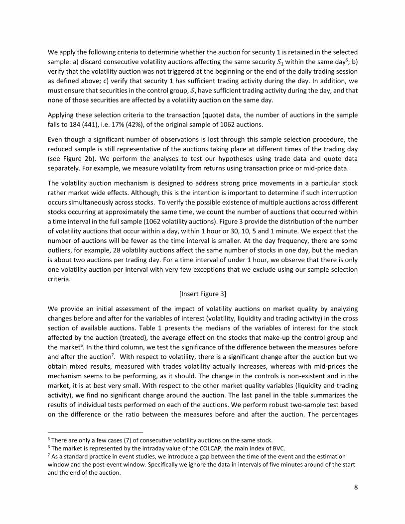
We apply the following criteria to determine whether the auction for security 1 is retained in the selected

sample: a) discard consecutive volatility auctions affecting the same security 𝑆1 within the same day5; b)

verify that the volatility auction was not triggered at the beginning or the end of the daily trading session

as defined above; c) verify that security 1 has sufficient trading activity during the day. In addition, we

must ensure that securities in the control group, 𝒮, have sufficient trading activity during the day, and that

none of those securities are affected by a volatility auction on the same day.

Applying these selection criteria to the transaction (quote) data, the number of auctions in the sample

falls to 184 (441), i.e. 17% (42%), of the original sample of 1062 auctions.

Even though a significant number of observations is lost through this sample selection procedure, the

reduced sample is still representative of the auctions taking place at different times of the trading day

(see Figure 2b). We perform the analyses to test our hypotheses using trade data and quote data

separately. For example, we measure volatility from returns using transaction price or mid-price data.

The volatility auction mechanism is designed to address strong price movements in a particular stock

rather market wide effects. Although, this is the intention is important to determine if such interruption

occurs simultaneously across stocks. To verify the possible existence of multiple auctions across different

stocks occurring at approximately the same time, we count the number of auctions that occurred within

a time interval in the full sample (1062 volatility auctions). Figure 3 provide the distribution of the number

of volatility auctions that occur within a day, within 1 hour or 30, 10, 5 and 1 minute. We expect that the

number of auctions will be fewer as the time interval is smaller. At the day frequency, there are some

outliers, for example, 28 volatility auctions affect the same number of stocks in one day, but the median

is about two auctions per trading day. For a time interval of under 1 hour, we observe that there is only

one volatility auction per interval with very few exceptions that we exclude using our sample selection

criteria.

[Insert Figure 3]

We provide an initial assessment of the impact of volatility auctions on market quality by analyzing

changes before and after for the variables of interest (volatility, liquidity and trading activity) in the cross

section of available auctions. Table 1 presents the medians of the variables of interest for the stock

affected by the auction (treated), the average effect on the stocks that make-up the control group and

the market6. In the third column, we test the significance of the difference between the measures before

and after the auction7. With respect to volatility, there is a significant change after the auction but we

obtain mixed results, measured with trades volatility actually increases, whereas with mid-prices the

mechanism seems to be performing, as it should. The change in the controls is non-existent and in the

market, it is at best very small. With respect to the other market quality variables (liquidity and trading

activity), we find no significant change around the auction. The last panel in the table summarizes the

results of individual tests performed on each of the auctions. We perform robust two-sample test based

on the difference or the ratio between the measures before and after the auction. The percentages

5 There are only a few cases (7) of consecutive volatility auctions on the same stock. 6 The market is represented by the intraday value of the COLCAP, the main index of BVC. 7 As a standard practice in event studies, we introduce a gap between the time of the event and the estimation window and the post-event window. Specifically we ignore the data in intervals of five minutes around of the start and the end of the auction.

9

indicate the number of auctions where we reject the null hypothesis that the measures are statistically

equivalent using the sample data before and after the auction. A higher percentage indicated that there

are more auctions where the variables of interest change around the auction. The percentage tends to be

higher in the treated variable than in the control or the overall market.

[Insert Table 1]

5. Synthetic portfolio method

Event studies is one of the most widely used methodologies in accounting and financial research (Kothari

and Warner, 2005), and in certain legal proceedings. The timeline structure of an event study has not

changed dramatically since its introduction in the late sixties (Ball and Browm, 1968). There are important

number of contributions that have focused specially on providing better tools for statistical inference, see

Corrado (2011) for a recent discussion. A recurrent element in event studies is the use of the market

model to estimate the so call “normal” returns. In fact, Corrado (2011) argues that the popularity of event

studies stems from a coincidence of developments in financial market research in the late 60’s: CAPM,

the CRISP data and more sophisticated and accessible statistical software.

In traditional event studies (MacKinlay, 1997), the effect of a particular event on a stocks’s price is

measured by the abnormal returns (ARs). For simplicity, suppose that stock 1 is the only security affected

by an event, the abnormal return is:

𝐴𝑅1,𝑡 = 𝑅1,𝑡 − 𝐸[𝑅1,𝑡|𝑋𝑡], 𝑡 ∈ (𝑇0, 𝑇] (1)

where 𝑅1,𝑡 is the actual return and 𝐸[𝑅1,𝑡|𝑋𝑡] is the expected normal return. There are two common

choices for modeling the expected return: the constant mean return model and the market model. In both

cases researchers use information in the pre-event window to quantify the normal return. In the constant

mean return model, the normal return is the simple average of the variable of interest in the pre-event

window. In the market model, the normal return is given by, [𝑅1,𝑡|𝑋𝑡] = �̂�𝑅𝑚,𝑡, where 𝑅𝑚,𝑡 is the excess

market return at time 𝑡 and �̂� is the estimated slope in the following regression, estimated with data in

the pre-event window.

𝑅1,𝑡 = 𝛼𝑖 + 𝛽𝑖𝑅𝑚,𝑡 + 𝜖1,𝑡. (2)

For the event study, we perform on the volatility auctions we follow a different approach that deviates

from the use of the market model or the constant mean model to build the expected normal return. The

main reason to deviate from the traditional approach is that we consider the expected return as a

potential outcome. Taking that point of view, we try adapting existing methods in causal inference, in

particular synthetic control methods (introduced by Abadie, Diamond and Hainmuller, 2010) to the

problem at hand.

The synthetic control method (Abadie, Diamond and Hainmuller, 2010), has received a lot of attention in

comparative case studies on different subjects: terrorism, natural disasters, and tobacco control

programs. As opposed to competing methods, synthetic control method's strength relies in the use of a

combination of units to build a more objective comparison for the unit exposed to the intervention, rather

than a choosing a single unit or an Ad hoc reference group. The authors advocate for the use of data drive

10

procedures to build the reference group. The synthetic control method is a weighted average of the

available control units, which makes explicit: the contribution of each unit to the counterfactual of interest

and the similarities (or lack thereof) between the units affected by the event or the intervention of interest

and the synthetic control in terms of the pre-intervention outcomes and other predictors of post-

intervention outcomes.

Synthetic matching techniques applied for event studies in finance are not common, we are only aware

of their application in a recent paper, Acemoglu, Johnson, Kermani and Kwak (2016). In this paper, the

authors measure the effect of personal connections on the returns of financial firms. The study is based

on the connections of Timothy Geithner to different financial institutions prior to his nomination as

Treasury Secretary at the end of 2008. The authors use a synthetic matching methodology to complement

to the usual approach in event studies of capturing the difference between a treatment and control group

using for the latter the fitted market model.

We illustrate the synthetic matching methodology using an event study methodology with a synthetic

portfolio as measure of the normal returns. The event of interest is the volatility auction, and our purpose

is to determine the causal effect of such a market mechanism on market quality variables after continuous

trading is resumed.

We denote 𝑡 as the intraday time (1 < 𝑡 < 𝑇) and 𝑇0 as the time when the auction takes place. Although,

the auction lasts for approximately two and a half minutes, for notational simplicity we denote this

interval as a particular moment in time, 𝑇0. The pre-event or estimation window is defined by 𝑡 ∈ [1, 𝑇0),

and the post-event or forecast window is defined by 𝑡 ∈ [𝑇0, 𝑇). The main challenge in determining the

causal effect of the volatility auction (the intervention) on a given stock is the construction of a potential

outcome or counterfactual. This tries to capture what would have happened to the stock return had the

volatility auction not taken place.

The available data is intra-day data of the securities of interest 𝑌𝑖,𝑡 for stock 𝑖 = 1,… , 𝐽 and, 𝑡 =

1,… , 𝑇 where 𝑇0 < 𝑇. Suppose that stock 1 is the only one affected by the intervention, that is 𝑌1,𝑡

receives the treatment and the rest of the stock (𝑌2,𝑡, … . , 𝑌𝐽,𝑡) are in the control group. Let 𝑌𝑖,𝑡𝑁 (𝑌𝑖,𝑡

𝐼 )

denote the outcome that would be (is) observed for stock 𝑖 if the volatility auction had not taken (takes)

place at time, 𝑇0. Note that 𝑌𝑖,𝑡𝑁 is a latent variable and 𝑌𝑖,𝑡

𝐼 is the observed outcome for the variable of

interest after the intervention (𝑇0 < 𝑡 < 𝑇).

In our application and similar to traditional event studies, the variable of interest is stock returns (𝑌𝑖,𝑡 ≔

𝑅𝑖,𝑡). Therefore, 𝑅1,𝑡 is the return of the stock whose trading has been halted because of the volatility

auction (the stock that has been treated). Conversely, the synthetic portfolio is built using the other

securities (those in continuous trading before and after the intervention) to replicate the performance of

the security of interest.

The methodology is very simple because we only need to obtain the portfolio weights 𝑤𝑗∗ by solving the

optimal tracking problem,

𝑤∗ = 𝑎𝑟𝑔𝑚𝑖𝑛𝑤∑(𝑌1,𝑡 −∑𝑤𝑗

𝐽

𝑗=2

𝑌𝑗,𝑡)

2

, (5)

𝑇0

𝑡=1

11

for the estimation window ∈ [1, 𝑇0) . The optimization is constrained because weights must sum to

one(∑ 𝑤𝑗𝐽𝑗=2 = 1). It is possible to include in this optimization problem additional restrictions on the

estimated weights, for example non-negativity constraints8.

A proper tracking of the stock of interest would guarantee that the synthetic portfolio could provide a

potential outcome for the latent variable 𝑅1,𝑡𝑁 in the post event window (𝑇0, 𝑇]9.

The effect of the intervention is equivalent to the abnormal returns of the asset of interest,

�̂�1,𝑡 = 𝐴𝑅1,𝑡 = 𝑅1,𝑡 − 𝑅1,𝑡𝑁 = 𝑅1,𝑡 −∑𝑤𝑗

∗

𝐽

𝑗=2

𝑅𝑗,𝑡 , 𝑡 ∈ (𝑇0, 𝑇] . (6)

As indicated previously, traditional economic and financial event studies provides two approaches to

quantify the latent return 𝑅1,𝑡𝑁 usually denoted as the normal return. The intent is to capture the usual

behavior or the return in the absence of the intervention; the approaches are the constant mean return

model or the market model. It is possible think of both approaches in a more general framework. The first

approach only considers lagged time-series information from the stock on the return of interest in the

estimation window (𝑅1,1, … . 𝑅1,𝑇0−1) to estimate, 𝑅1,𝑡𝑁 . Lagged time series information with equal weights

assigned to all observations is the usual approach known as the constant mean return model. It is also

possible to use a different weighting to come up with a different version of the estimate for 𝑅1,𝑡𝑁 ; for

example it would be quite natural to assume that return follow a stationary AR(1) process and use the

estimated coefficients (the first autocorrelation) to obtain the desired estimate of the potential

outcome10. The more popular approach is to use the market model or some other factor model (Fama-

French three-factor or Carhart four factor model). This is actually very close to the original idea of a

synthetic control (Abadie, et al. 2010), where the data generating process of 𝑅1,𝑡𝑁 is determined by a factor

model11. In finance factor models are used in many application, and although there is an extensive

literature, there is also an important discussion on the validity of the factors used to explain the cross

section of returns (Harvey, Liu and Zhu, 2015).

Event studies in finance are observational studies rather than perfectly randomized experiments. In these

types of studies, one way to strengthen the validity of the results is to guarantee that any decision on the

research design is independent from the possible effects that such decisions may have on the conclusions

of the study (Rubin, 2004). This implies that the methods preferably do not require strong assumption on

the post event outcomes. The potential outcomes are generally considered as missing variables in the

causal inference literature because it is not possible to observe all the instances of the variable of interest

8 Later we compare the performance of the restricted (non-negative weights) and the unrestricted weights. 9 The goodness of fit of the matching is determined by estimating the Mean Square Error in the estimation window or by testing that the cumulative abnormal returns are not statistically different form zero. 10 The AR(1) process can be justified on the basis of the effects of the bid-ask spread bouce on the price process, (Roll 1984). 11 Abadie et al. (2010) treat the potential outcome problem as a missing data one and therefore define a data generating process for the missing outcome. The choice is a factor model that includes observed covariates and unobserved components. Both elements are unit specific (for each stock) and are not time varying. The implementation of synthetic control methods for the present case is not straightforward because there are no unit specific controls relevant for the sampling frequency.

12

simultaneously. In many financial event studies, the researcher only observed the treated observation.

Estimation of potential outcomes in observational studies uses one of the following techniques or a

combination of some of them (Imbens and Rubin, 2015): model based-imputation, weighting, blocking

and matching methods. In model-based imputation, the researcher builds a model in order to predict the

missing potential outcome of unit that is not treated. This is exactly what traditional event studies do

when they define the normal returns using the constant return model or the market model. Model based

imputation is not recommended to estimate treatment effects because a proper fit can only be

accomplished by specifying the post-event outcomes. Weighting and blocking use the propensity score to

combine the information of the control units in order to build a proper counterfactual12. Using the

propensity score achieves a balance between treated and control groups in order to estimate an unbiased

treatment effect. Matching techniques find direct comparisons or matches for each unit. For a given

treated unit with a particular value for the covariates, one searches for a control unit with similar values

in the covariates. A distance metric is needed to implement a matching technique to assess the trade-off

in choosing between different units and/or controls.

The synthetic matching or synthetic portfolio approach can be considered an alternative way of defining

a normal return model, which avoids strong assumptions on the effects of treatment or non-treatment.

The synthetic portfolio method is very general, and does not require a natural experiment or ad hoc

criteria to select the securities in the control group; therefore, researchers can use it in many types of

event studies. One advantage of synthetic matching over traditional methods is the use of a different set

of securities than the security of interest, the treated observation, which avoids any interference of the

event on the potential outcome of interest. Under perfect circumstances, there is a well-defined control

group. Off course, one must take care in avoiding any hidden variation that might spill over from the event

to the control group13.

The synthetic portfolio approach has an important difference with respect to synthetic control method: it

has no covariates. Covariates are not used because the matching is based strictly on the ability of the

combination the stocks in the control group to perform an adequate tracking of the treated stock in the

estimation window. As mentioned previously the most natural way to introduce covariates in this context

is to use a factor model14. This implies a trade-off between a model with tighter restriction on the

matching of units with the use of covariates and a miss specification problem brought on by the model or

the wrong covariates15. It is possible to use discrete value covariates (indicator functions that signal

whether a stock belongs to a group of assets with similar characteristics), for example industry

classification. However, this is equivalent to using industry indexes in the factor model rather than the

12 The propensity score is the average unit assignment (for a particular treatment) probability for units that share the same specific characteristic. 13 One could argue that the market model does also provide a way to avoid the used of the treated variable in the construction of the potential outcome; this is true because one would expect that in a liquid and deep market the security of interest is only one of many constituents of the index. This is however not necessarily true for thinly traded markets where the index can be determined mostly by a handful of assets. For example, by early August 2010, four stocks of the twenty that constitute the COLCAP made up 56% of the index value. 14 Unfortunately the most commonly used factor models in finance (Fama-French three-factor or Carhart four factor model) do not use unit specific covariates, which impedes the “off-the-shelf” use of synthetic control methods. 15 For the time being, it is not clear how to find a good trade off in an estimator; Imbens (2015) provides a discussion and recommendations in a general context.

13

market index. For the application to the volatility auctions, the number of feasible stock used to analyze

each action is not enough to classify into industry portfolios or any other classification.

[Insert Figure 4]

Figure 4 provides a graphical illustration of how synthetic portfolio method works. The continuous line

shows the observed evolution of returns for security 1 before and after the event, while the dash line

shows the evolution of the synthetic portfolio. Note that in the pre-event window, the synthetic portfolio

performs well in tracking the performance of security 1, as it clearly replicates the return on the security

of interest16. Thus, we have a strong proxy for security 1 just before the volatility auction. Once the

volatility auction is complete and a new equilibrium price is obtained, continuous trading resumes in the

post-event window and we see the evolution of the returns on security 1 that have been affected or

treated by the volatility auction. Thus, the post-event return on the synthetic portfolio 𝑅P,𝑡 ≔

∑ 𝑤𝑗∗𝐽

𝑗=2 𝑅𝑗,𝑡 becomes a proxy for the unobserved potential outcome in relation to security 1 had the

volatility auction not taken place (𝑅1,𝑡𝑁 ) , in other words the state in which security 1 is not exposed to the

volatility auction (the treatment). We emphasize that none of the securities in the synthetic portfolio are

affected by the volatility auction, and thus have received no treatment. It is important to note the effects

of the sample selection criteria over the estimated effect of the intervention. That is, the effect of the

sample selection criteria that we impose on the elements of the control group regarding the no inclusion

of stocks that have a similar type of volatility auction over the trading day. The main reason to include this

criterion is to avoid any interference in the measure by using a very strict condition on being part of the

control group. However, this creates a censoring of the potential outcome because these stocks never

have price paths that excess the limits defined by the mechanism. This implies that by censoring the

potential outcome (the synthetic portfolio) we measure a lower bound for the effect with respect to the

non-censored case. Therefore, the effect of the intervention measured in terms of the abnormal returns

of stock 1 (𝐴𝑅1,𝑡) is a conservative lower bound for the true uncensored effect.

In order to map returns to volatility of stock 1 and the synthetic portfolio in the pre-event and port-event

window, we obtain five-minute realized volatility and perform nonparametric two-sample scale test on

the differences between these volatilities for each auction. These tests help us in determining: first,

whether there is good tracking performance in the estimation window with respect to the variable of

interest and that the estimated volatilities are equivalent (two-sided test). Second, whether the volatility

auction mechanism is working, and the volatility of the non-treated (the synthetic portfolio) is significantly

larger than the treated unit (stock 1), for this we use a one-sided test. We also follow the suggestion of

Abadie, et al. (2010) and form a placebo test for the synthetic matching. The purpose of the placebo test

is to randomize treatment within the units of analysis (stock 1 and the stocks in the control group) that

are trading at the same time. This exercise allows us to determine whether the estimated effect of the

volatility auction (on stock 1) is large relative to the distribution of the effects estimated on for the stocks

in the control group that are not exposed to the interruption. We perform these last tests in the post-

event window.

16 It is possible to use several test to evaluate tracking performance in the estimation window, for example using the root mean square error or a test of hypothesis on the tracking error, which is actually equivalent to testing the cumulative abnormal returns. The null hypothesis of the test would be that the tracking error or the cumulative abnormal returns are equal to zero.

14

We use the weights of the synthetic portfolio, to build synthetic indicators of the other variables of

interest (bid–ask spreads, depth, and turnover). We can generalize the previous measure of abnormal

returns to a measure of the effects of a volatility auction on any of the variables that are informative with

respect to market quality:

𝛿1,𝑡 = 𝑌1,𝑡 − 𝑌Ρ,𝑡

= 𝑌1,𝑡 −∑𝑤𝑗∗

𝐽

𝑗=2

𝑌𝑗,𝑡 𝑡 ∈ (𝑇0, 𝑇]. (4)

Since most of the indicators of market quality have a strictly positive support, we use weights of the

synthetic portfolio returns based on the restricted estimator (weights are non-negative, 𝑤𝑗∗ ≥ 0). We do

not perform a separate matching procedure for each variable, because we do not have a large number of

assets in the control group and hence imposing non-negativity constraint on the weights usually leads to

selecting one of the stocks. When the methodology only select one of the stocks, the tracking

performance is very poor and hence we rather use the weights obtained from tracking returns.

We also perform hypothesis test on the pre-event and post-event outcomes of the other variables of

interest (bid–ask spread, turnover). For all of the variables and the results that we present in the following

sections we only use volatility auctions where there is good tracking performance (in the estimation

window) based on these test strategies to determine the effectiveness of the mechanism and its effect

on market quality.

6. Empirical analysis

a. The synthetic portfolio

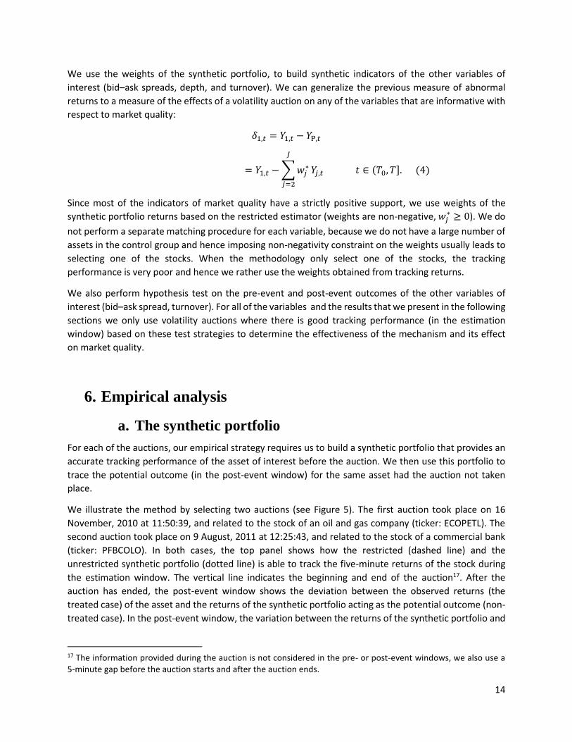
For each of the auctions, our empirical strategy requires us to build a synthetic portfolio that provides an

accurate tracking performance of the asset of interest before the auction. We then use this portfolio to

trace the potential outcome (in the post-event window) for the same asset had the auction not taken

place.

We illustrate the method by selecting two auctions (see Figure 5). The first auction took place on 16

November, 2010 at 11:50:39, and related to the stock of an oil and gas company (ticker: ECOPETL). The

second auction took place on 9 August, 2011 at 12:25:43, and related to the stock of a commercial bank

(ticker: PFBCOLO). In both cases, the top panel shows how the restricted (dashed line) and the

unrestricted synthetic portfolio (dotted line) is able to track the five-minute returns of the stock during

the estimation window. The vertical line indicates the beginning and end of the auction17. After the

auction has ended, the post-event window shows the deviation between the observed returns (the

treated case) of the asset and the returns of the synthetic portfolio acting as the potential outcome (non-

treated case). In the post-event window, the variation between the returns of the synthetic portfolio and

17 The information provided during the auction is not considered in the pre- or post-event windows, we also use a 5-minute gap before the auction starts and after the auction ends.

15

the observed returns in both stocks is expected to be significant because the counterfactual is designed

to capture an unobserved state wherein the auction did not take place.

[Insert Figure 5]

One advantage of using intraday data is that, compared with daily data, there is less chance of introducing

a confounding effects unrelated to the volatility auction. Furthermore, the construction of the

counterfactual using a synthetic portfolio is more robust. Compared with other approaches used in

comparative case studies, we are not choosing one particular asset or reference group of assets to build

the counterfactual, but rather we are using an optimal set of weights to replicate the asset of interest

using a control group that has not been affected by the auction. Although there are bound to be some

externalities from informationally related securities, as identified by Jian, McInish, and Upson (2009), our

approach is a less biased alternative because the weights are estimated rather than imposed. The bottom

panels in Figure 5 show the estimated weights that are used to build the synthetic portfolio in the two

auctions, for both the restricted (𝑤 >= 0) and the unrestricted case (𝑤 free). Each asset in the control

group receives a positive or negative weight. The asset does not necessarily belong to a specific asset class

that has similar characteristics to the asset affected by the auction. For example, in some comparative

case studies, Guidolin and La Ferrara (2007), the authors build the control group by choosing companies

in the same sector. The synthetic portfolio is only built on the notion that a particular asset in the control

group (not treated by the volatility auction) provides a contribution to tracking the asset of interest (the

stock that will be affected by the volatility auction) before the realization of the event of interest (the

volatility auction).

In table 2, we look at the performance of synthetic portfolio in both the estimation as well as the post-

event window. In the top left panel we compare the performance of the synthetic portfolio method

against the traditional event study methods (time series or market model approach) using the root mean

square error (RMSE) between the observed and the estimated returns along the estimation window. We

find that the synthetic portfolio does not provide a better alternative when trying to fit the returns of the

asset of interest, all the more when using unrestricted weights. However, we are not interested in testing

cumulative abnormal returns, which is equivalent to looking at the RMSE, rather we are interested in

testing the difference between the volatilities of the treated unit and the synthetic portfolio in the

estimation window. Good tracking performance will guarantee a replication of the volatility by the

synthetic portfolio with respect to the treated unit. In the top right panel, we provide the percentage of

auctions where we can reject the null hypothesis that the volatilities are different between the volatility

of the treated and the non-treated. The results indicate a slight advantage of synthetic control methods

(less rejections) for the same set of auctions.

In the two lower panels of Table 2, we look at the performance of synthetic portfolio in the post-event

window. We use the placebo test proposed by Abadie et al. (2010) to look at the robustness of the results.

The idea is that the estimated effect of non-treatment, in this case no auction, the volatility is larger in

magnitude than in the case where there is a randomized treatment over the control units and the

treatment unit (including it in the portfolio). The results indicate the percentage of auctions where the

volatility of the synthetic after the auction is above the 95th percentile of the placebo distribution. If this

is so then the magnitude of the effect is well above the randomization of the treatments over all units.

The percentage of auctions that overcome the placebo test is 36 to 42% of the auctions analyzed. Imposing

non-negativity contains in the weights creates a significant reduction in auctions that pass the placebo-

16

test and hence we concentrate on the results for the unrestricted case but making sure that the matching

is adequate for volatility in the estimation window.

[Insert Table 2]

b. Impact of volatility auctions on volatility

To assess the impact of the volatility auction on volatility, following the methodology outlined in the

previous section, we estimate five-minute realized volatilities for the treated stock and for the non-

treated control (the synthetic portfolio) both before and after the auction. We are only using auctions

where the synthetic portfolio has a good tracking performance of the asset of interest in the pre-event

window. If hypothesis 1 is correct and the volatility auction avoids large price variations, the asset that

has gone into the auction (treated) displays lower volatility than the potential outcome captured by the

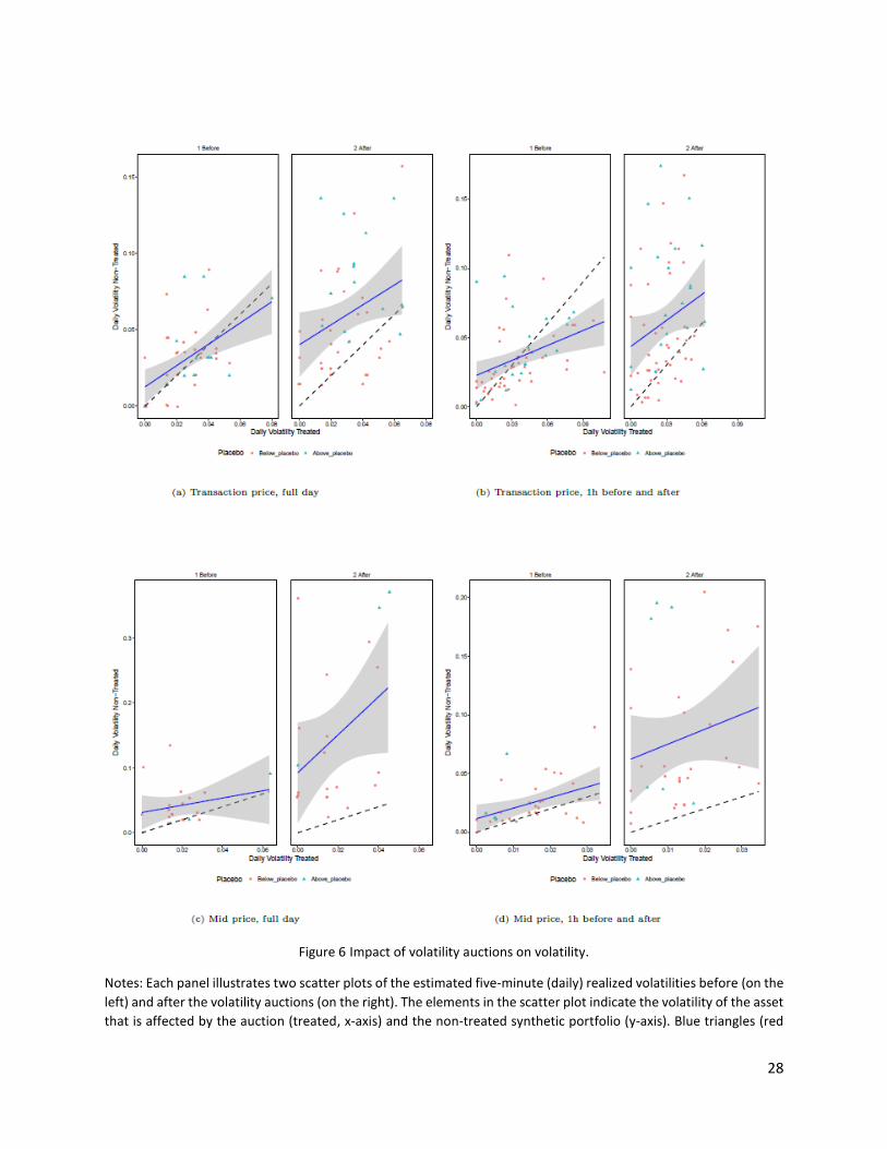
synthetic (non-treated) portfolio, after the auction. In figure 6, we capture the average effect using the

cross section of volatilities for the auctions. There are two panels in every figure. The left panel is a scatter

plot of the treated and non-treated units before the auction. A black dashed line represents the case

where the volatility of the non-treated is exactly equal to the volatility of the treated. In other words, the

line has a zero intercept and a slope exactly equal to one. The blue solid line represents the estimated OLS

fitting line and the gray area the corresponding 95th confidence interval. A perfect matching before the

auction would require that the solid line coincides with the dashed line on that the intercept and the slope

of the estimated solid is statistically equal to zero and one, respectively. This is not the case in any of the

right panels, but in general the matching is close enough and the dashed line is mainly within or close to

the gray area. This is the best match we can accomplish given that we are already using the subset of

auctions where we cannot reject the null hypothesis that the estimated realized volatilities are equivalent

before the auction.

In the right panel of each figure, we use the same auctions and present the observed volatility of the

treated unit after the auction and the volatility of the synthetic portfolio using the estimated weights and

the observed return process for the stocks belonging to the control group (no treatment). This is our

estimate of what would have happened to the volatility had the auction not taken place. The estimated

line based on these set of points will give us a rough estimate of the average effect of the volatility auction

mechanism. In particular, we look at the difference between the intercept of both blue solid curves before

and after the auction as the measure of the effect of the volatility auction. This measure is between 3%

and 6% less volatility in the stocks subject to volatility auctions, in other words this is 10 to 25 times larger

than what we see in the average data before and after the auction (Table 1).

Alternatively, in Table 3 we look at the difference in the medians and perform a two-sample Wilcoxon test

on the data points for the treated and non-treated units. The average effect of the volatility auction is

between 1.2% and 8% less volatility after continues trading resumes (first column of Table 3). Using the

data just one hour before and after the auction the effect is between 2.2% and 4%.

[Insert Figure 6]

Looking at the plots in Figure 6, the top and bottom panels differ in terms of the information used to

estimate the returns and volatilities, i.e. transaction prices versus mid-prices. The right and left panels

17

differ in terms of the amount of five-minute returns used to estimate the realized volatilities. In the left

panels, all of the information in both the pre- and post-event windows is used18. In the right panels, we

only consider five-minute returns for one hour before and after the auction. In all of the four panels of

Figure 6, we observe that the volatility auction delivers a relative reduction in volatility, which is in line

with the results for the German Xetra stock market (Gombet et al., 2011; Zimmerman, 2013) and Spanish

stock market (Reboredo, 2010)19.

From the results of table 3, in general we find that the volatility of the treated stock after the auction does

not change whereas the volatility of the non-treated always increases and the increase is statistically

significant. Only in one case, volatility based on trades using all available data, we find that the volatility

is increasing in both the treated and the non-treated synthetic, but the last one in a greater amount (more

than twice). Because we are not exploring the specific causes of the increase in volatility that triggered

the auction, our conclusions on the performance of the volatility auction mechanism assume that it

mitigates volatility spikes in individual stocks (by a reduction or bounding) and not in the overall market.

The additional evidence presented in figure 3 regarding the low occurrence of multiple auctions does not

indicate that the auctions are triggered by systemic effects in the market. However, it´s still plausible that

a peak in the market volatility will only affect one stock with a combination of high beta and high

idiosyncratic volatility relative to the predefined price range20.

[Insert Table 3]

c. Impact of volatility auctions on liquidity

Similar to volatility, we measure the effect of volatility auctions on other variables of market quality for

both treated stocks and the corresponding synthetic portfolios. Figure 7 shows the change in the bid–ask

spread for the two groups. The top graphs show the results for the effective bid–ask spread, while the

bottom graphs show the results for the quoted bid–ask spread, both of which are defined in Goyenko,

Holden, and Trzcinka (2009). As before, the left panels use all the available information on the trading

day, while the right panels only use information from one hour before and after the call auction. It is

apparent that the volatility auction does not have a significant effect on the bid–ask spread for the treated

stock, as the circles are reasonably evenly distributed above and below the black line in all four cases.

Interestingly, the liquidity measure seems to decrease after the call auction for the non-treated group, as

the circles tend to be below the black line in all four panels. These preliminary results clearly refute the

hypothesis that volatility auctions improve the liquidity of the treated stocks.

18 Note that the amount of available information can differ because it depends on the time when the auction takes place during the trading day. 19 We performed robustness tests based on one-minute and 10-minute returns and the results were equivalent with respect to the effectiveness of the mechanism, the only significant difference being that in some cases we had a smaller number of feasible auctions to analyze, and thus tracking performance declined at these frequencies. These results are available upon request to the authors. 20 The difficulty lies in the fact that in order to disentangle systemic and idiosyncratic volatility we have to make strong assumption in the data generating process and in particular the effect on the potential outcome. This is however contrary to our initial motivation of making few assumptions as possible to arrive at an estimate of the potential outcome.

18

[Insert Figure 7]

Table 3 also includes the median of the measures of liquidity and trading activity for both groups, before

and after the auction. We include five liquidity measures: the quoted and effective spreads, the depths at

both quotes, and the ratio of the bid–ask spread to average depth, as presented by Jiang et al. (2009).

Focusing on the results with all of the available data (columns 1 and 2), there is a reduction in the quoted

bid–ask spread in both groups, significant at the 5% level, and also in the spread/depth ratio. Moreover,

there is a statistically significant reduction in the effective bid–ask spread in the control group, but not in

the treated stock. This minor increase in liquidity in both the stock and the synthetic portfolio can be

attributed to the well-known trend whereby liquidity improves during the trading day. In turn, there is a

significant drop on the bid depth of the treated stock, but the opposite effect for the synthetic portfolio.

In terms of trading activity, measured by the turnover, there is no significant effect on either the stock

undergoing the auction (treated) or the synthetic portfolio (non-treated). Overall, the results in Table 3

do not support hypothesis 2. Thus, the volatility auction does not have a discernible effect on the market

quality variables of the treated stock other than volatility itself.

7. Conclusions

In this paper, we address one of the main difficulties in event studies: building a credible counterfactual.

Traditional event studies have focused on using the security of interest fitted to the market model

(MacKinlay, 1997), building a reference group based on assets with similar characteristics or behavior

(Jiang et al., 2009), or defining pseudo-events (Reboredo, 2010; Abad and Pascual, 2010).

We suggest a different methodological approach by proposing a synthetic portfolio for event studies. This

approach allows us to build a more general and robust counterfactual. Our counterfactual is the best

tracking portfolio for the stock of interest, obtained as a weighted average of the returns on the stocks

that have not been affected by the event. The methodology has enormous potential for overcoming some

common problems in event studies, such as confounding effects and the fact that in small stock markets

it is not easy to find enough stocks with a particular characteristic to build a control group. In addition,

there are some obstacles to overcome in the methodology, for example, we do not explore the role of

covariates that are widely accepted as very important for matching in causal inference. One possibility

that we hope to explore in a follow-up paper, is that given the connection to portfolio optimization we

can try to use parametric portfolio policies (Brandt, Santa-Clara and Valkanov, 2009) to introduce

covariates in the weights and explore the benefit of such strategies.

We use the synthetic portfolio method to test the effectiveness of a type of circuit breaker known as a

volatility auction. We use high-frequency TAQ data from the BVC, which uses this mechanism in its trading

platform.

Studying volatility auctions observed over a two-year period from 2010 to 2012, we find positive results

in terms of the effectiveness of the mechanism, which has a significant impact in terms of mitigating

excessive volatility during the trading day. In addition, we do not find any effect on other dimensions of

market quality such as liquidity, depth, and trading activity.

19

References

Abadie, A., Diamond, A., Hainmuller, J. (2010). “Synthetic control methods for comparative case studies:

Estimating the effect of California’s tobacco control program”, Journal of the American Statistical

Association, 105(490), pp.493-505.

Abad, D., Pascual, R. (2010). “Switching to a temporary call auction in times of high uncertainty”, Journal

of Financial Research, 35(1), pp.45-75.

Acemoglu, D., Johnson, S., Kermani, A., Kwak, A., Mitton, T. (2016). “The Value of Connections in Turbulent

Times: Evidence from the United States”, Journal of Financial Economics, 121, pp.368-391.

Agarwalla, S. K., Jacob, J., & Pandey, A. (2015). Impact of the introduction of call auction on price discovery: Evidence from the Indian stock market using high-frequency data. International Review of Financial Analysis, 39, 167-178.

Ball, R. and Brown, P. (1968). An empirical evaluation of accounting income numbers. Journal of Accounting Research, 6, 159-178.

Brandt, M.W., Santa-Clara, P. and Valkanov, R. “Parametric Portfolio Policies: exploiting the cross section of equity returns”, The Review of Financial Studies, 22(9), pp.3411-3447.

Bekaert, G., & Harvey, C. R. (2002). Research in emerging markets finance: looking to the future. Emerging Markets Review, 3(4), 429-448.

Bildik, R., & Gülay, G. (2006). Are price limits effective? Evidence from the Istanbul Stock Exchange. Journal of Financial Research, 29(3), 383-403.

Chan, S. H., Kim, K. A., & Rhee, S. G. (2005). Price limit performance: evidence from transactions data and the limit order book. Journal of Empirical Finance, 12(2), 269-290.

Cho, D. D., Russell, J., Tiao, G. C., & Tsay, R. (2003). The magnet effect of price limits: evidence from high-frequency data on Taiwan Stock Exchange. Journal of Empirical Finance, 10(1), 133-168.

Christie, W.G., Corwin, S.A., Harris, J.H. (2002). “Nasdaq trading halts: The impact of market mechanisms

on prices, trading activity, and execution costs”, Journal of Finance, 57, pp. 1443-1478.

Comerton-Forde, C. (1999). Do trading rules impact on market efficiency? A comparison of opening procedures on the Australian and Jakarta Stock Exchanges. Pacific-Basin Finance Journal, 7(5), 495-521.

Corrado, J. C. (2011). “Event studies: A methodology review”, Accounting and Finance, 51, 207-234.

Corwin, S. A., Lipson, M. L. (2000). “Order flow and liquidity around NYSE trading halts”, Journal of Finance,

55(4), pp. 1771-1801.

Dalko, V.(2016). Limit Up–Limit Down: an effective response to the “Flash Crash”?. Journal of Financial

Regulation and Compliance, 24(4), 420-429.

European Commission, (2010). “Public consultation, review of the markets in financial instruments

directive (mifid)”. Available at:

http://ec.europa.eu/finance/consultations/2010/mifid/docs/consultation_paper_en.pdf

20

Fama, E.F. (1989). “Perspectives on October 1987, Or, What Did We Learn from the Crash?”. In SR.W.

Kamphuis, Jr., R.C. Kormendi, and J.W.H. Watson. (Eds). Black Monday and the Future of Financial Markets

(pp.71-82). Chicago: Mid America Institute for Public Policy Research.

Farag, H. (2015). The influence of price limits on overreaction in emerging markets: Evidence from the Egyptian stock market. The Quarterly Review of Economics and Finance, 58, 190-199.

Francioni, R., (2013). Chapter 2: “Mid Day Address”. In Schawrz.R.A, Byerne, J.A and Schnee, G. (Eds). The

Quality of our Financial Market. Taking stock of where we stand (pp.17-27). New York, NY: Springer.

Frino, A., Lecce, S., and Segara, R. (2011). “The impact of trading halts on liquidity and price volatility:

Evidence from the Australian Stock Exchange”, Pacific Basin Finance Journal, 19, pp. 298-307.

Gerace, D., Liu, Q., Tian, G. G., & Zheng, W. (2015). Call auction transparency and market liquidity:

Evidence from china. International Review of Finance, 15(2), 223-255.

Glosten, L. R., and Milgrom, P. R. (1985). “Bid, ask and transaction prices in a specialist market with

heterogeneously informed traders”, Journal of Financial Economics, 14(1), pp. 71-100.

Gomber, P. (2016). “The German Equity Trading Lanscape”. Available at:

http://safefrankfurt.de/fileadmin/user_upload/editor_common/Policy_Center/Gomber_Equity_Trading.

pdf

Gomber, P., Lutat, M., Haferkorn, M., Zimmermann, K. (2011). “The effect of single-stock circuit breakers

on the quality of fragmented markets”. Lecture Notes in Business Information Processing, 136, 71-87.

Goyenko, R. Y., Holden, C. W., and Trzcinka, C. A. (2009). “Do liquidity measures measure liquidity?”,

Journal of Financial Economics, 92(2), pp. 153-181.

Gow, I.D., Larcker, D.F., Reiss, P.C. (2016). “Causal inference in accounting research”. Working paper series

No. 217, Rock Center for Corporate Governance, Stanford University.

Greenwald, B.C. and J.C. Stein. (1988). “The Task Force Report: The Reasoning Behind the

Recommendations”, Journal of Economic Perspectives, 2, pp. 3-23.

Greenwald, B.C. and J.C. Stein. (1991). “Transactional Risk, Market Crashes, and the Role of Circuit

Breakers”, Journal of Business, 64, pp. 443-462.

Grossman, S.J. (1990). “Introduction to NBER Symposium on the October 1987 Crash”. Review of Financial

Studies, 3, pp. 1-3.

Grundy, B.D. and McNichols, M. (1989). “Trade and revelation of information through prices and direct

disclosure”. Review of Financial Studies, 2, pp. 495-526.

Guidolin, M., La Ferrara, E. (2007). “Diamonds Are Forever, Wars Are Not: Is Conflict Bad for Private

Firms?”, The American Economic Review, 97(5), pp.1978-1993.

Harvey, C.R., Liu, Y., Zhu, H. (2016). “… and the cross-section of expected returns”, The Review of Financial Studies, 29:5-68.

21

Huang, Y. S. (1998). Stock price reaction to daily limit moves: evidence from the Taiwan stock exchange. Journal of Business Finance & Accounting, 25(3‐4), 469-483.

Huang, Y. S., Fu, T. W., & Ke, M. C. (2001). Daily price limits and stock price behavior: evidence from the Taiwan stock exchange. International Review of Economics & Finance, 10(3), 263-288.

Imbens, G.W. (2015). “Matching Methods in Practice: Three Examples”. Journal of Human Resources,

March 31, 2015 50:373-419.

Imbens, G.W. and Rubin, D.B. (2015). Causal inference for statistics, social and biomedical sciences: an

introduction. New York, NY: Cambridge University Press.

Jiang, C., McInish, T., Upson, J. (2009). “The information content of trading halts”, Journal of Financial

Markets, 12, pp.703-726.

Kim, K. A. (2001). Price limits and stock market volatility. Economics Letters, 71(1), 131-136.

Kim, Y. H., Yage, J., and Yang, J. J. (2008). “Relative performance of trading halts and price limits: Evidence

from the Spanish Stock Exchange”, International Review of Economics and Finance, 17, pp.197-215.

Kim, Y. H., and Yang, J. J. (2004). “What Makes Circuit Breakers Attractive to Financial Markets? A Survey”,

Financial Markets, Institutions and Instruments, 13(3), pp.109-146.

Kirilenko, A., Kyle, A. S., Samadi, M., & Tuzun, T. (2017). The Flash Crash: High‐Frequency Trading in an

Electronic Market. Journal of Finance, 72(3), 967-998.

Kryzanowski, L., and Nemiroff, H. (1998). “Price discovery around trading halts on the Montreal Exchange

using trade-by-trade data”, Financial Review, 33, pp.195-212.

Kyle, A. S. (1985). “Continuous Auctions and Insider Trading”, Econometrica, 53(6), p.1315-1335.

Kothari, S.P. and Warner, J.B. (2005), Econometrics of event studies, in: B. Eckbo Espen, ed., Handbook of

Corporate Finance: Empirical Corporate Finance (Handbooks in Finance Series, Elsevier, North-Holland),

3-36.

Lee, C. M. C., Ready, M. J., and Seguin, P. J (1994). “Volume, Volatility, and New York Stock Exchange

Trading Halts”, Journal of Finance, 49(1), pp.183-214.

MacKinlay, A.C. (1997). “Event studies in economics and finance”, Journal of Economic Literature,

35(March), pp.13-39.

Madhavan A. (1992). “Trading Mechanisms in Securities Markets”, Journal of Finance, 47(2), pp.607-641.

Nath, P. (2005). Are price limits always bad?. Journal of Emerging Market Finance, 4(3), 281-313.

Pagano, M.S., Peng, L., Schwartz, R. (2013). “A call auction’s impact on price formation and order routing:

Evidence from the NASDAQ stock market”, Journal of Financial Markets, 16, pp.331-361.

Reboredo J. (2012). “The switch from continuous to call auction trading in response to a large intraday

price movement”, Applied Economics, 44(8), pp.945-967.

Roll , R. (1984). “A simple implicit measure of the effective bid-ask spread in an efficient market”, The

Journal of Finance, Vol. XXXIX, No. 4, September, pp.1127-1139.

22

Rubin, D.B. (2004). “Causal inference using potential outcomes: Design, Modeling, Decisions”, Fisher

Lecture, The Journal of the American Statistical Association, Vol. 100(469): 322-331.

Spiegel, M. and Subrahmanyam A. (2002). “Asymmetric information and news disclosure rules”, Journal

of Financial Intermediation , 9, pp.363-403.

Subrahmanyam A. (1994). “Circuit Breakers and Market Volatility: A Theoretical Perspective”, Journal of

Finance, 49(1), pp.237-254.

Subrahmanyam, A. (2013). Algorithmic trading, the Flash Crash, and coordinated circuit breakers. Borsa

Istanbul Review, 13(3), 4-9.

Zimmermann, K. (2013). “Price Discovery in European Volatility Interruptions”. Available

at:http://www.fese.eu/images/documents/deLaVega/PriceDiscoveryinEuropeanVolatilityInterruptions.p

df.

23

Figures and Tables

Figure 1 Volatility auction mechanism.

Source: BVC.

24

Figure 2 Volatility auctions identified from August 2010 to August 2012.

25

Figure 3 Number of volatility auctions within a predefined time interval.

Notes: The time interval are: during the trading day (Day), within 1 hour (1hr), or within 30,10,5 or 1 minute(s).

26

Figure 4 Synthetic portfolio method for event studies in market microstructures.

27

Figure 5 Synthetic portfolio.

Notes: Panels (a) and (b) illustrate the five-minute observed returns (solid line), synthetic returns with portfolio

weights above or equal to zero (dashed line) and synthetic returns with unrestricted portfolio weights (dotted line)

of ECOPETL and PFBCOLO over the trading day. We observed a call auction (the event) taking place at the time

indicated by the red vertical line. The vertical line also determines the pre-event/estimation window and the post-

event/forecasting window. Panels (c) and (d) indicate the estimated weights of the synthetic portfolio for ECOPETL

and PFBCOLO. These weights are estimated using the observed returns in the pre-event window, for both the

restricted and the un-restricted portfolio optimization.

28

Figure 6 Impact of volatility auctions on volatility.

Notes: Each panel illustrates two scatter plots of the estimated five-minute (daily) realized volatilities before (on the

left) and after the volatility auctions (on the right). The elements in the scatter plot indicate the volatility of the asset

that is affected by the auction (treated, x-axis) and the non-treated synthetic portfolio (y-axis). Blue triangles (red

29

circles) indicate auctions where the post-event estimation of the volatility using the synthetic portfolio attain a value

above (below) the 95th percentile of the distribution over the placebo test. In each plot the dashed black line

indicates the curve under which the volatility of the treated and the non-treated is exactly the same. The solid blue

line is the OLS fitted line using the data points and the gray area is the 95th confidence interval around this line. If

the estimated solid blue line is close to the dashed line before the auction then we assume that the matching is

correct in the estimation window (before the auction). The solid blue lines estimated with the data points before

and after the action give an idea of the effect of the volatility auctions on the non-treated (potential outcome), that

is, a larger intercept after the auction (on the right) indicates the average volatility that would have been expected

had the auction not taken place. In panels (a) and (b), the realized volatilities are estimated using five-minute returns

based on mid-prices (quote data), whereas panels (c) and (d) provide estimated volatilities from trades. In panels (a)

and (c), the realized volatilities before and after the auction are measured using the continuous trading information

for the full day. In panels (b) and (d), the realized volatilities before and after the auction are measured using the

continuous trading information for only one hour before and after the auction.

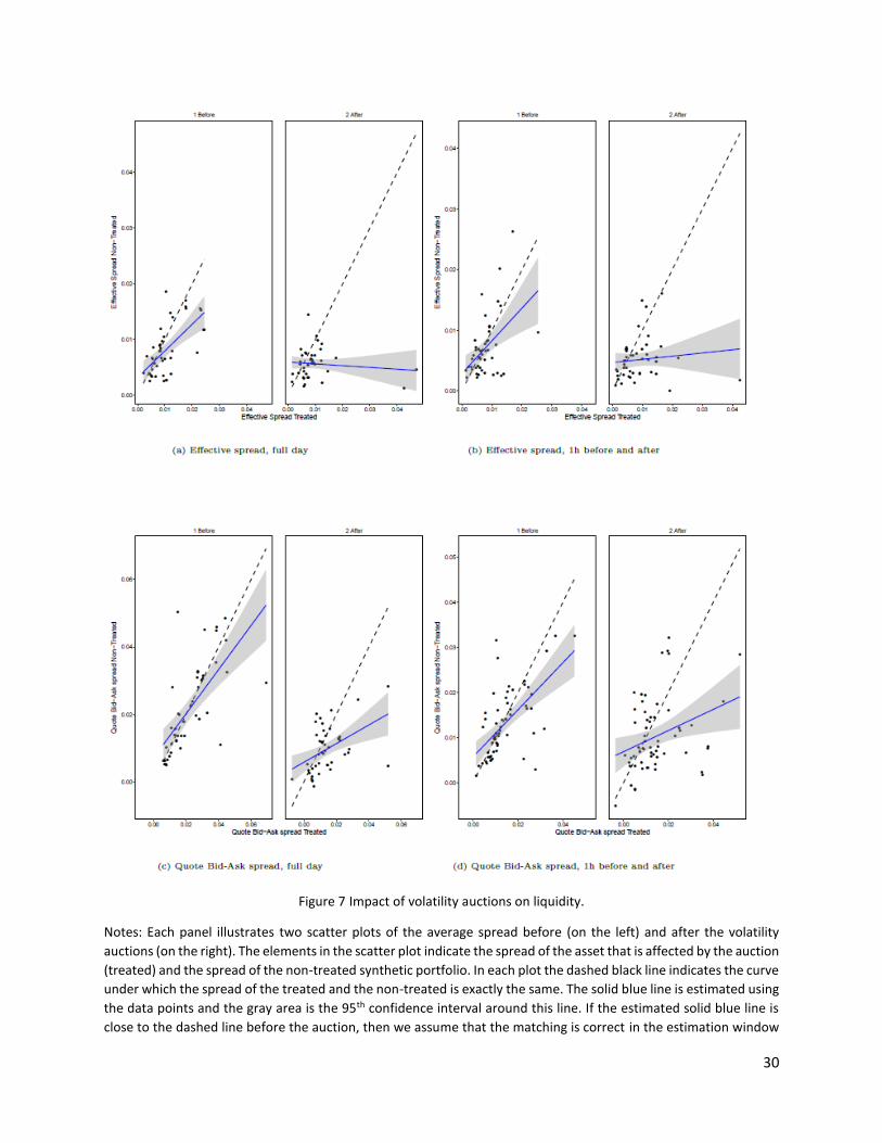
30

Figure 7 Impact of volatility auctions on liquidity.

Notes: Each panel illustrates two scatter plots of the average spread before (on the left) and after the volatility

auctions (on the right). The elements in the scatter plot indicate the spread of the asset that is affected by the auction

(treated) and the spread of the non-treated synthetic portfolio. In each plot the dashed black line indicates the curve

under which the spread of the treated and the non-treated is exactly the same. The solid blue line is estimated using

the data points and the gray area is the 95th confidence interval around this line. If the estimated solid blue line is

close to the dashed line before the auction, then we assume that the matching is correct in the estimation window

31

(before the auction). The estimated solid blue lines before and after the action provide a measure the effect of the

volatility auctions on the non-treated (potential outcome), that is, a larger intercept after the auction indicates a

wider average spread that would have been expected had the auction not taken place. In panels (a) and (b), the

spreads are measured using the effective spread based on transaction prices and quotes. In panels (c) and (d), the

spreads are measured using bid and ask prices (quote data). In panels (a) and (c), the average spreads before and

after the auction are measured using the continuous trading information for the full day. In panels (b) and (d), the

average spreads before and after the auction are measured using the continuous trading information for only one

hour before and after the auction.

32

33

Table 1 Descriptive Statistics of the variables of interest before and after the volatility auction.

Notes: The tables contain the medians on the variables of interest using the information for the sample of feasible auctions using the trade and quote data. The

table on the top used all the available information during the trading day before and after the auction, to compute the descriptive statistics. The table in the

bottom only considers the available information up until one hour before and after the volatility auction. The first two panels contain the median measures of

the variables of interest across all of the auctions before and after. Each of these set of columns has the information for the asset that is affected by the auction

(treated), the average value for the controls (the assets that are trading at the same time but are not affected by the volatility auction) and the relevant market

index (COLCAP). We use the cross section of actions to measure the difference between before and after the volatility auction (excluding a 5 minute interval

before and after). We use t-test and ratio test, to ascertain the statistical significance of the differences (*, **, and *** denote significance at the 10%, 5%, and

1% levels, respectively). In addition, for each individual auction we test the null hypothesis that each of the variables of interest is statistically equivalent before

and after the auction. In the last columns, we report the percentage of auctions where we can reject the null hypothesis indicating that the variables are

statistically equivalent before and after the volatility auctions.

Treated Controls Market Treated Controls Market Treated Controls Market Treated Controls Market

Average return Trades 0.03% 0.00% 0.01% 0.00% 0.00% 0.00% -0.03%** 0.00 0.00 0.13 0.11 0.14

Average return Mid-Price 0.00% 0.00% 0.00% 0.00% 0.00% 0.00% 0.00%* 0.00%* 0.00 0.21 0.09 0.11

Volatility (daily) Trades 2.35% 0.41% 0.46% 2.60% 0.37% 0.46% 0.25%** 0.00 0.00 0.61 0.43 0.34

Volatility (daily) Mid-Price 2.77% 0.62% 0.57% 1.90% 0.86% 0.49% -0.88%*** 0.00 -0.08%*** 0.76 0.71 0.48

Quote Bid-Ask Spread 1.80% 3.22% 1.44% 2.50% 0.00 -0.72%*** 0.72 0.93

Efective Spread 0.81% 0.74% 0.72% 0.57% 0.00 -0.17%*** 0.61 0.81

Bid Depth 38.12 93.65 32.85 102.97 -5.27 9.33*** 0.77 0.74

Ask Depth 44.53 102.42 51.83 115.51 7.30 13.09*** 0.84 0.71

Spread Depth 0.04% 0.06% 0.02% 0.05% -0.01%*** -0.02%*** 0.74 0.80

Turnover 32.11 29.01 24.47 27.97 -7.64 -1.04 0.59 0.66

Treated Controls Market Treated Controls Market Treated Controls Market Treated Controls Market

Average return Trades 0.02% 0.00% 0.00% 0.00% 0.00% 0.00% -0.02%*** -0.01% 0.00% 0.10 0.13 0.09

Average return Mid-Price 0.00% 0.00% 0.00% 0.00% 0.00% 0.00% 0.00% 0.00% 0.00% 0.33 0.09 0.08

Volatility (daily) Trades 2.54% 0.42% 0.50% 2.57% 0.41% 0.51% 0.03% -0.01% 0.01% 0.55 0.29 0.23

Volatility (daily) Mid-Price 1.69% 0.30% 0.51% 1.28% 0.28% 0.48% -0.41%** -0.02% -0.03%** 0.71 0.45 0.19

Quote Bid-Ask Spread 1.17% 2.97% 1.18% 2.80% 0.02% -0.17%*** 0.61 0.73

Efective Spread 0.64% 0.80% 0.68% 0.65% 0.03% -0.15%*** 0.46 0.81

Bid Depth 38.78 92.38 37.25 98.28 -1.53 5.90** 0.62 0.37

Ask Depth 49.54 101.98 49.37 108.41 -0.16 6.43* 0.58 0.43

Spread Depth 0.03% 0.06% 0.02% 0.05% 0.00% -0.01%*** 0.57 0.63

Turnover 30.45 29.47 24.38 29.70 -6.07 0.23 0.40 0.59

Information for all day of trading

1 hour before and after auction

Before auction After auction Difference % of Auctions

Before auction After auction Difference % of Auctions

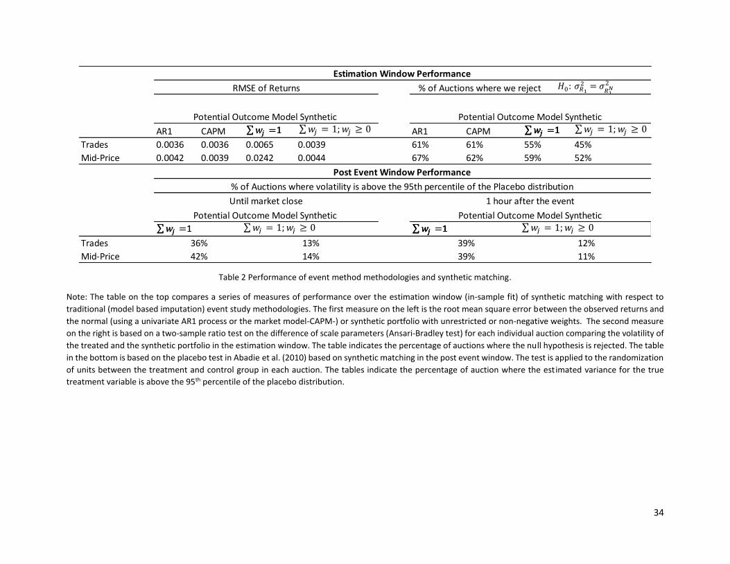
34

Table 2 Performance of event method methodologies and synthetic matching.

Note: The table on the top compares a series of measures of performance over the estimation window (in-sample fit) of synthetic matching with respect to

traditional (model based imputation) event study methodologies. The first measure on the left is the root mean square error between the observed returns and

the normal (using a univariate AR1 process or the market model-CAPM-) or synthetic portfolio with unrestricted or non-negative weights. The second measure

on the right is based on a two-sample ratio test on the difference of scale parameters (Ansari-Bradley test) for each individual auction comparing the volatility of

the treated and the synthetic portfolio in the estimation window. The table indicates the percentage of auctions where the null hypothesis is rejected. The table

in the bottom is based on the placebo test in Abadie et al. (2010) based on synthetic matching in the post event window. The test is applied to the randomization

of units between the treatment and control group in each auction. The tables indicate the percentage of auction where the estimated variance for the true

treatment variable is above the 95th percentile of the placebo distribution.

AR1 CAPM AR1 CAPM

Trades 0.0036 0.0036 0.0065 0.0039 61% 61% 55% 45%

Mid-Price 0.0042 0.0039 0.0242 0.0044 67% 62% 59% 52%

Trades

Mid-Price

39%

39%

12%

11%

36%

42%

13%

14%

Post Event Window Performance

% of Auctions where volatility is above the 95th percentile of the Placebo distribution

Until market close 1 hour after the event

Potential Outcome Model Synthetic Potential Outcome Model Synthetic

% of Auctions where we reject

Potential Outcome Model Synthetic Potential Outcome Model Synthetic

Estimation Window Performance

RMSE of Returns

∑𝑤𝑗 =1 ∑𝑤𝑗 = 1 𝑤𝑗 ≥ 0∑𝑤𝑗 =1 ∑𝑤𝑗 =1 ∑𝑤𝑗 = 1 𝑤𝑗 ≥ 0∑𝑤𝑗 =1∑𝑤𝑗 =1

0 2 =

2

∑𝑤𝑗 =1 ∑𝑤𝑗 = 1 𝑤𝑗 ≥ 0∑𝑤𝑗 =1 ∑𝑤𝑗 =1 ∑𝑤𝑗 = 1 𝑤𝑗 ≥ 0∑𝑤𝑗 =1∑𝑤𝑗 =1

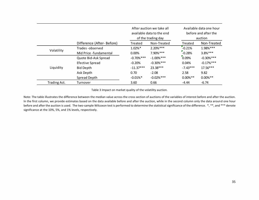
35

Table 3 Impact on market quality of the volatility auction.

Note: The table illustrates the difference between the median value across the cross section of auctions of the variables of interest before and after the auction.

In the first column, we provide estimates based on the data available before and after the auction, while in the second column only the data around one hour

before and after the auction is used. The two-sample Wilcoxon test is performed to determine the statistical significance of the difference. *, **, and *** denote

significance at the 10%, 5%, and 1% levels, respectively.

Difference (After- Before) Treated Non-Treated Treated Non-Treated

Trades -observed 1.02%* 2.20%*** -0.21% 1.98%***

Mid Price -fundamental 0.00% 7.90%*** -0.28% 3.8%***

Quote Bid-Ask Spread -0.70%*** -1.00%*** 0.09% -0.30%***

Efective Spread -0.20% -0.30%*** 0.04% -0.17%***

Bid Depth -11.37*** 23.38*** -7.43*** 17.56***

Ask Depth 0.70 -2.08 2.58 9.82

Spread Depth -0.01%* -0.02%*** 0.00%** 0.00%**

Trading Act. Turnover 3.60 0.66 -4.44 -6.74

After auction we take all

available data to the end

of the trading day

Available data one hour

before and after the

auction

Volatility

Liquidity