Embed Size (px)
Citation preview
Measuring the Point Spread Function of aLight Microscope
by
Anthony D. Patire
Submitted to the Department of Electrical Engineering and
Computer Science
in partial fulfillment of the requirements for the degree of
Master of Engineering in Electrical Engineering and Computer Science
at the
MASSACHUSETTS INSTITUTE OF TECHNOLOGY
February 1997
@ Massachusetts Institute of Technology, MCMXCVII.
All rights reserved.I CN
Signature of Author .............. .. .. ...... - ...........
Department of Electrical Engineering and Computer Science
February 7, 1997
Certified by ... . ...
Dennis M. Freeman
Assistant Professor of Electrical Engineering
r Thesis Supervisor
Accepted by V ........ I .- - ..............."t:s f., Frederic R. Morgenthaler
Chairman Department Committee on Graduate ThesesMAR 2 11997
LIBRARIES
aI a
Measuring the Point Spread Function of a Light Microscope
by
Anthony D. Patire
Submitted to the
Department of Electrical Engineering and Computer Science
February 7, 1997
In Partial Fulfillment of the
Requirements for the Degree of
Master of Engineering in Electrical Engineering and Computer Science
ABSTRACT
Methods are described to measure the impulse response, or point spread function
(PSF), of a light microscope. The new methods compare favorably to those used by
others, which are shown to be flawed. The new methods measure a three-dimensional
point target in both fluorescence and brightfield microscopy using K6hler illumination.
The results closely match theoretical predictions. Simple theory does not capture all
of the behavior of the microscope. A qualitative extension to the theory is given to
explain discrepancies between measurements and theoretical predictions that occur in
some operating regimes of the microscope.
Thesis Supervisor: Dennis Freeman
Title: Assistant Professor of Electrical Engineering

Acknowledgments
First, I would like to thank Denny Freeman for advising me throughout this thesis.
His friendly encouragement was always appreciated and his enthusiasm was often
contagious. I would also like to thank Zoher, Rosanne, Quentin, Laura, Cameron,
and A.J. for their insight, laughter, sarcasm, patience, cynicism, and beer. It was
a pleasure to work with a group of people who are even more disturbed than I am.
Special thanks to Denny, A.J., Laura, and Rosanne for proofreading my thesis and
offering countless suggestions and improvements. Thanks for the really great emu!
I would like to thank all my friends, past and present-you know who you are.
Thank you Allen and Carrie for standing by me under the wrath of a malevolent taxi
cab driver. I owe a great deal to my family without whom none of this would have
been possible. Thank you mom, dad, grandmom, and grandpop for sending me to
M.I.T., and thank you Mary, for being the best sister a brother could possibly have.
I rolled the dice, and I won. Thank you, God.
Contents
1 Introduction
2 Background on Optical Microscopy
2.1 Kbhler Illumination and Fourier Optics . . . . . . . . . . . . . . . . .
2.2 PSF Model Based on Diffraction Limited Optics . . . . . . . . . . . .
2.3 Experimental Determination of Model Parameter . . . . . . . . . . . .
3 Methods
3.1 Measuring the PSF ...........
3.1.1 Experimental Setup: Overview .
3.1.2 Sampling the Image .......
3.1.3 Two-Dimensional Step Target .
3.1.4 Three-Dimensional Point Target
3.2 Data Analysis ..............
3.2.1 Two-Point Correction ......
3.2.2 Normalization and Statistics . .
3.3 Index of Refraction of Gel . . . . . . .
4 Results
4.1 Repeatability of Measurements .....
4.2 Fluorescence Microscopy ........
4.3 Brightfield Microscopy .........
4.3.1 Effect of Microsphere Size . . .
15
... . 15
. . . . 15
. . . . 15
. . . . 16
. . . . 17
... . 19
. . . . 19
. . . . 20
. . . . 20
23
. . . . . . . . . . . . . . . 23
. . . . . . . . . . . . . . . 25
..... ... .... ... 27
. . . . . . . . . . . . . . . 27
4.3.2 Effect of Condenser Iris NA
4.4 Effect of Aberrations ........
4.4.1 Chromatic Aberration....
4.4.2 Spherical Aberration ....
4.5 Comparison of Results to Theory .
4.6 Index of Refraction of Gel .....
5 Discussion
5.1 Repeatability of Measurements . ...
5.2 Fluorescence Microscopy .......
5.3 Brightfield Microscopy ........
5.3.1 Effect of Microsphere Size
5.3.2 Effect of Condenser Iris NA
5.4 Effect of Aberrations .........
5.4.1 Chromatic Aberration .....
5.4.2 Spherical Aberration .....
5.5 Comparison of Results to Theory . .
5.6 Bright Spot: A Possible Explanation
..... ........ .... ..... ... .. 4 7
. . . . . . . . . . . . . . . . . . . 27
................... 33
................... 33
................... 33
. . . . . . . . . . . . . . . . . . . 37
................... 39
.................. 4 1
.................. 42
S . . . . . . . . . . . . . . . . . 42
.................. 43
.................. 44
.................. 44
.................. 44
S . . . . . . . . . . . . . . . . . 45
S . . . . . . . . . . . . . . . . . 46
5.7 Conclusion ....
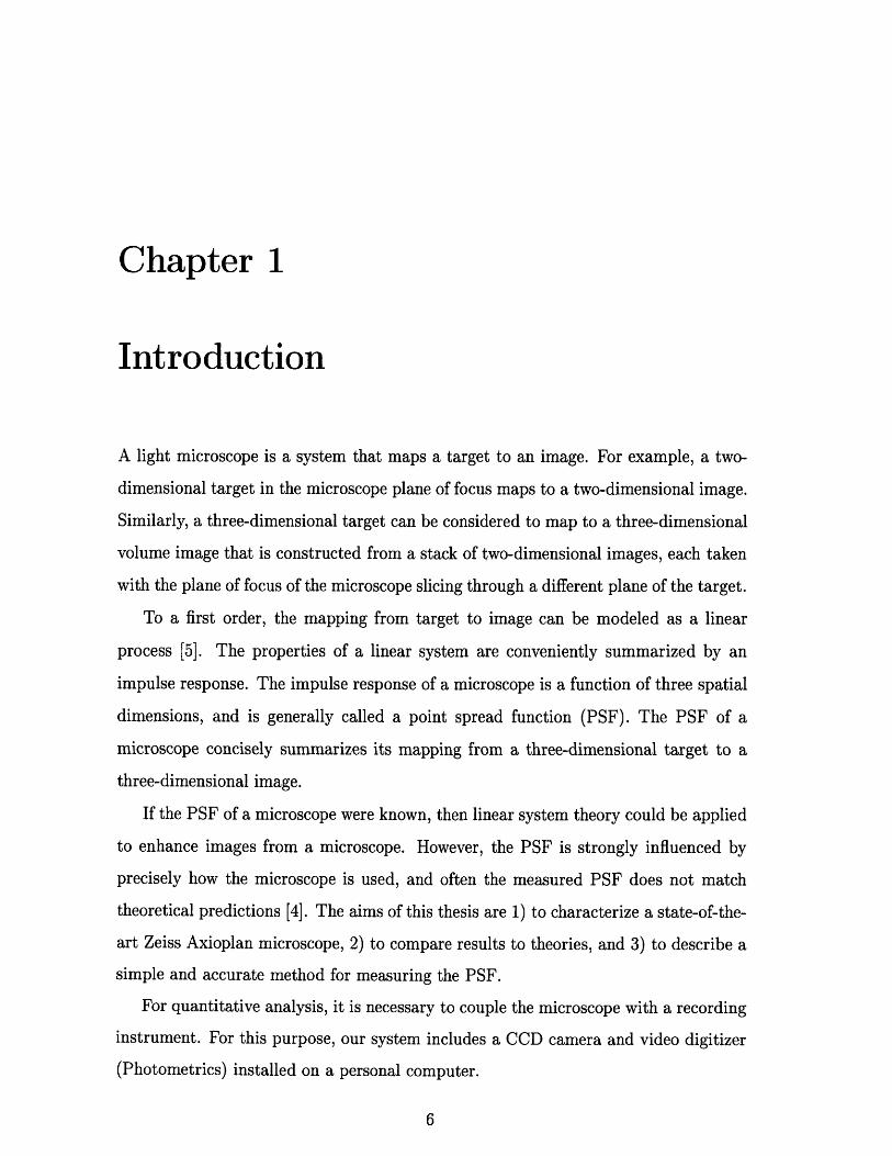
Chapter 1
Introduction
A light microscope is a system that maps a target to an image. For example, a two-
dimensional target in the microscope plane of focus maps to a two-dimensional image.
Similarly, a three-dimensional target can be considered to map to a three-dimensional
volume image that is constructed from a stack of two-dimensional images, each taken
with the plane of focus of the microscope slicing through a different plane of the target.
To a first order, the mapping from target to image can be modeled as a linear
process [5]. The properties of a linear system are conveniently summarized by an
impulse response. The impulse response of a microscope is a function of three spatial
dimensions, and is generally called a point spread function (PSF). The PSF of a
microscope concisely summarizes its mapping from a three-dimensional target to a
three-dimensional image.
If the PSF of a microscope were known, then linear system theory could be applied
to enhance images from a microscope. However, the PSF is strongly influenced by
precisely how the microscope is used, and often the measured PSF does not match
theoretical predictions [4]. The aims of this thesis are 1) to characterize a state-of-the-
art Zeiss Axioplan microscope, 2) to compare results to theories, and 3) to describe a
simple and accurate method for measuring the PSF.
For quantitative analysis, it is necessary to couple the microscope with a recording
instrument. For this purpose, our system includes a CCD camera and video digitizer
(Photometrics) installed on a personal computer.

Chapter two provides a basic background on optical microscopy. Kbhler Illumin-
ation and Fourier Optics are introduced as well as a basic microscope model from
which the theoretical PSF can be derived. Chapter three describes the important con-
siderations and the different processes for measuring the PSF. Both the procedures
for constructing a suitable test target, and the evaluation of raw data is explained.
Chapter four illustrates the various measurements of the PSF in both brightfield and
fluorescence microscopy. The features of these PSFs are compared to the theoretical
model. Chapter five discusses the significance of these findings, and evaluates the
consistency of the results.
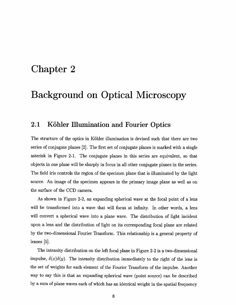
Chapter 2
Background on Optical Microscopy
2.1 Kohler Illumination and Fourier Optics
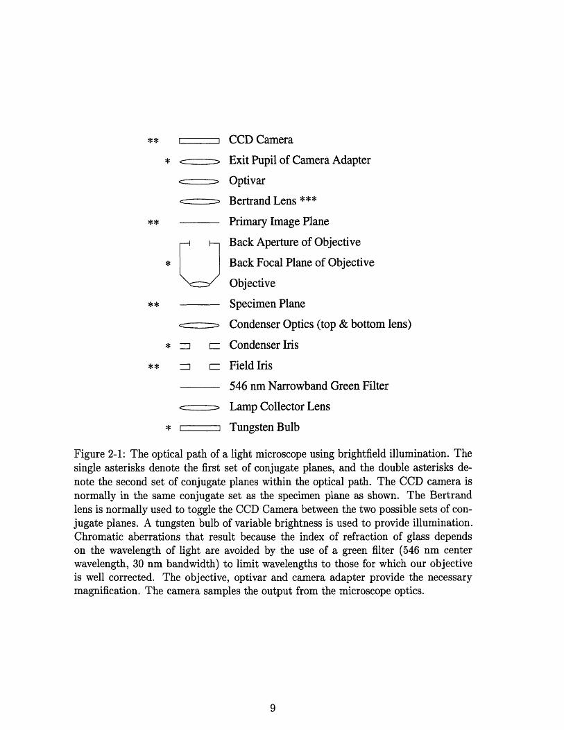
The structure of the optics in Kihler illumination is devised such that there are two
series of conjugate planes [2]. The first set of conjugate planes is marked with a single
asterisk in Figure 2-1. The conjugate planes in this series are equivalent, so that
objects in one plane will be sharply in focus in all other conjugate planes in the series.
The field iris controls the region of the specimen plane that is illuminated by the light
source. An image of the specimen appears in the primary image plane as well as on
the surface of the CCD camera.
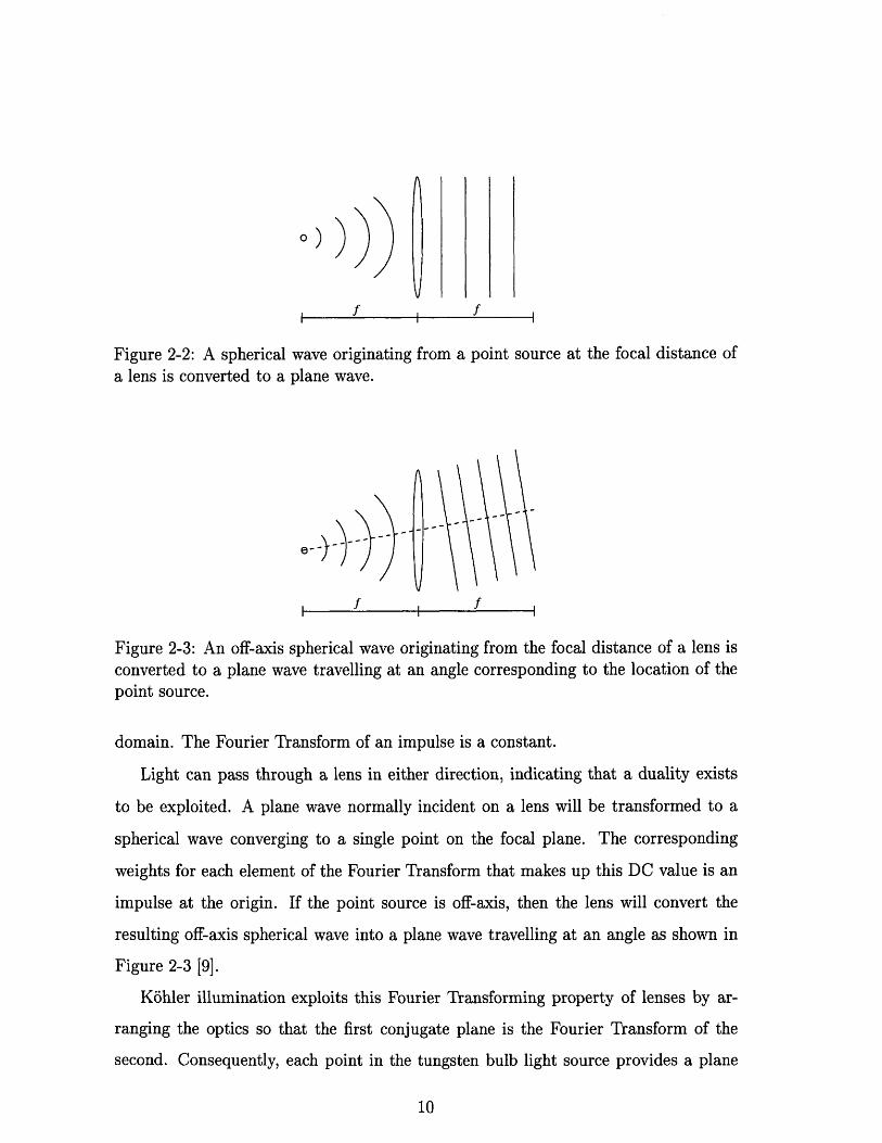
As shown in Figure 2-2, an expanding spherical wave at the focal point of a lens
will be transformed into a wave that will focus at infinity. In other words, a lens
will convert a spherical wave into a plane wave. The distribution of light incident
upon a lens and the distribution of light on its corresponding focal plane are related
by the two-dimensional Fourier Transform. This relationship is a general property of
lenses [5].
The intensity distribution on the left focal plane in Figure 2-2 is a two-dimensional
impulse, 5(x)6(y). The intensity distribution immediately to the right of the lens is
the set of weights for each element of the Fourier Transform of the impulse. Another
way to say this is that an expanding spherical wave (point source) can be described
by a sum of plane waves each of which has an identical weight in the spatial frequency
** CCD Camera
* • Exit Pupil of Camera Adapter
a Optivar
a Bertrand Lens ***
** Primary Image Plane
Back Aperture of Objective
Back Focal Plane of Objective
Objective
** Specimen Plane
z Condenser Optics (top & bottom lens)
* ie Condenser Iris
** - - Field Iris
546 nm Narrowband Green Filter
: Lamp Collector Lens
, I I Tungsten Bulb
Figure 2-1: The optical path of a light microscope using brightfield illumination. Thesingle asterisks denote the first set of conjugate planes, and the double asterisks de-note the second set of conjugate planes within the optical path. The CCD camera isnormally in the same conjugate set as the specimen plane as shown. The Bertrandlens is normally used to toggle the CCD Camera between the two possible sets of con-jugate planes. A tungsten bulb of variable brightness is used to provide illumination.Chromatic aberrations that result because the index of refraction of glass dependson the wavelength of light are avoided by the use of a green filter (546 nm centerwavelength, 30 nm bandwidth) to limit wavelengths to those for which our objectiveis well corrected. The objective, optivar and camera adapter provide the necessarymagnification. The camera samples the output from the microscope optics.
a))
f f
Figure 2-2: A spherical wave originating from a point source at the focal distance ofa lens is converted to a plane wave.
e-j)
f fSJ I
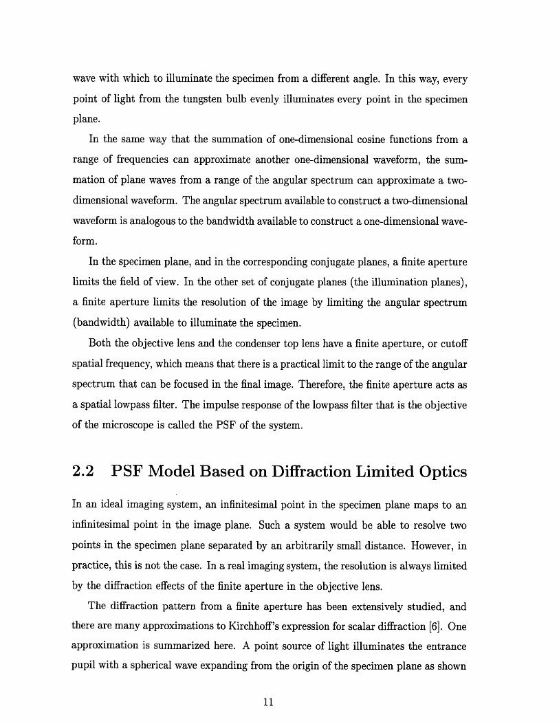
Figure 2-3: An off-axis spherical wave originating from the focal distance of a lens isconverted to a plane wave travelling at an angle corresponding to the location of thepoint source.
domain. The Fourier Transform of an impulse is a constant.
Light can pass through a lens in either direction, indicating that a duality exists
to be exploited. A plane wave normally incident on a lens will be transformed to a
spherical wave converging to a single point on the focal plane. The corresponding
weights for each element of the Fourier Transform that makes up this DC value is an
impulse at the origin. If the point source is off-axis, then the lens will convert the
resulting off-axis spherical wave into a plane wave travelling at an angle as shown in
Figure 2-3 [9].
Kdhler illumination exploits this Fourier Transforming property of lenses by ar-
ranging the optics so that the first conjugate plane is the Fourier Transform of the
second. Consequently, each point in the tungsten bulb light source provides a plane
I
wave with which to illuminate the specimen from a different angle. In this way, every
point of light from the tungsten bulb evenly illuminates every point in the specimen
plane.
In the same way that the summation of one-dimensional cosine functions from a
range of frequencies can approximate another one-dimensional waveform, the sum-
mation of plane waves from a range of the angular spectrum can approximate a two-
dimensional waveform. The angular spectrum available to construct a two-dimensional
waveform is analogous to the bandwidth available to construct a one-dimensional wave-
form.
In the specimen plane, and in the corresponding conjugate planes, a finite aperture
limits the field of view. In the other set of conjugate planes (the illumination planes),
a finite aperture limits the resolution of the image by limiting the angular spectrum
(bandwidth) available to illuminate the specimen.
Both the objective lens and the condenser top lens have a finite aperture, or cutoff
spatial frequency, which means that there is a practical limit to the range of the angular
spectrum that can be focused in the final image. Therefore, the finite aperture acts as
a spatial lowpass filter. The impulse response of the lowpass filter that is the objective
of the microscope is called the PSF of the system.
2.2 PSF Model Based on Diffraction Limited Optics
In an ideal imaging system, an infinitesimal point in the specimen plane maps to an
infinitesimal point in the image plane. Such a system would be able to resolve two
points in the specimen plane separated by an arbitrarily small distance. However, in
practice, this is not the case. In a real imaging system, the resolution is always limited
by the diffraction effects of the finite aperture in the objective lens.
The diffraction pattern from a finite aperture has been extensively studied, and
there are many approximations to Kirchhoff's expression for scalar diffraction [6]. One
approximation is summarized here. A point source of light illuminates the entrance
pupil with a spherical wave expanding from the origin of the specimen plane as shown
OpticalPath
Axis
Entrance V ExitPupil Pupil
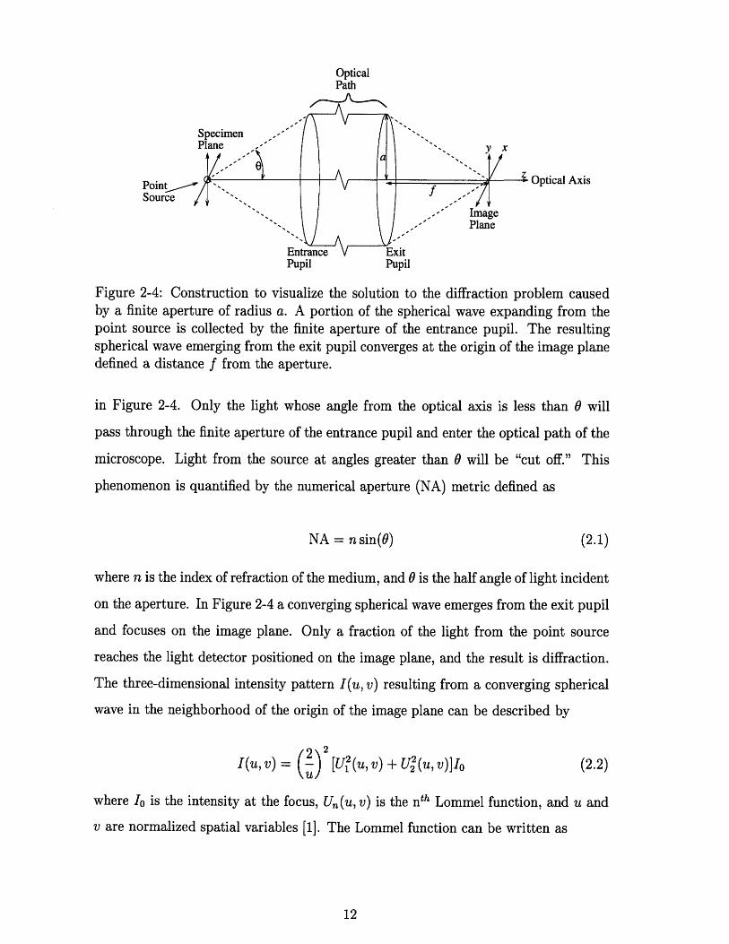
Figure 2-4: Construction to visualize the solution to the diffraction problem causedby a finite aperture of radius a. A portion of the spherical wave expanding from thepoint source is collected by the finite aperture of the entrance pupil. The resultingspherical wave emerging from the exit pupil converges at the origin of the image planedefined a distance f from the aperture.
in Figure 2-4. Only the light whose angle from the optical axis is less than 0 will
pass through the finite aperture of the entrance pupil and enter the optical path of the
microscope. Light from the source at angles greater than 0 will be "cut off." This
phenomenon is quantified by the numerical aperture (NA) metric defined as
NA = n sin(0) (2.1)
where n is the index of refraction of the medium, and 0 is the half angle of light incident
on the aperture. In Figure 2-4 a converging spherical wave emerges from the exit pupil
and focuses on the image plane. Only a fraction of the light from the point source
reaches the light detector positioned on the image plane, and the result is diffraction.
The three-dimensional intensity pattern I(u, v) resulting from a converging spherical
wave in the neighborhood of the origin of the image plane can be described by
I(u, v) = ( -) [U(, v) + U2(u, V)]I (2.2)
where Io is the intensity at the focus, U,,(u, v) is the nth Lommel function, and u and
v are normalized spatial variables [1]. The Lommel function can be written as
00 \ n+2sU,(u, v) = (-1)~ Jn+2.(v) (2.3)
8=0 V
where J, is the nt h order Bessel Function of the first kind, and the normalized spatial
variables are defined by
u = 2 ( z (2.4)A f
v = 2 + Y2 (2.5)
where a is the radius of the aperture, f is the focal distance of the lens, and A is the
optical wavelength of the light. The distribution of intensity is cylindrically symmetric
about the optical axis, and easy to visualize if only one axis is considered at a time.
Setting u = 0 in Equation 2.2 simplifies the expression into the familiar Airy formula,
I(0, v) = I) (2.6)
which describes the intensity of light in the geometrical focal plane (the image plane
orthogonal to the optical axis). Notice that it is circularly symmetric about the origin.
Setting v = 0 in Equation 2.2 simplifies the expression to
(sin(u/4)
(2.7)
I(u, 0) = ý u Io (2.7)
which describes the intensity distribution along the optical axis (orthogonal to the
image plane).
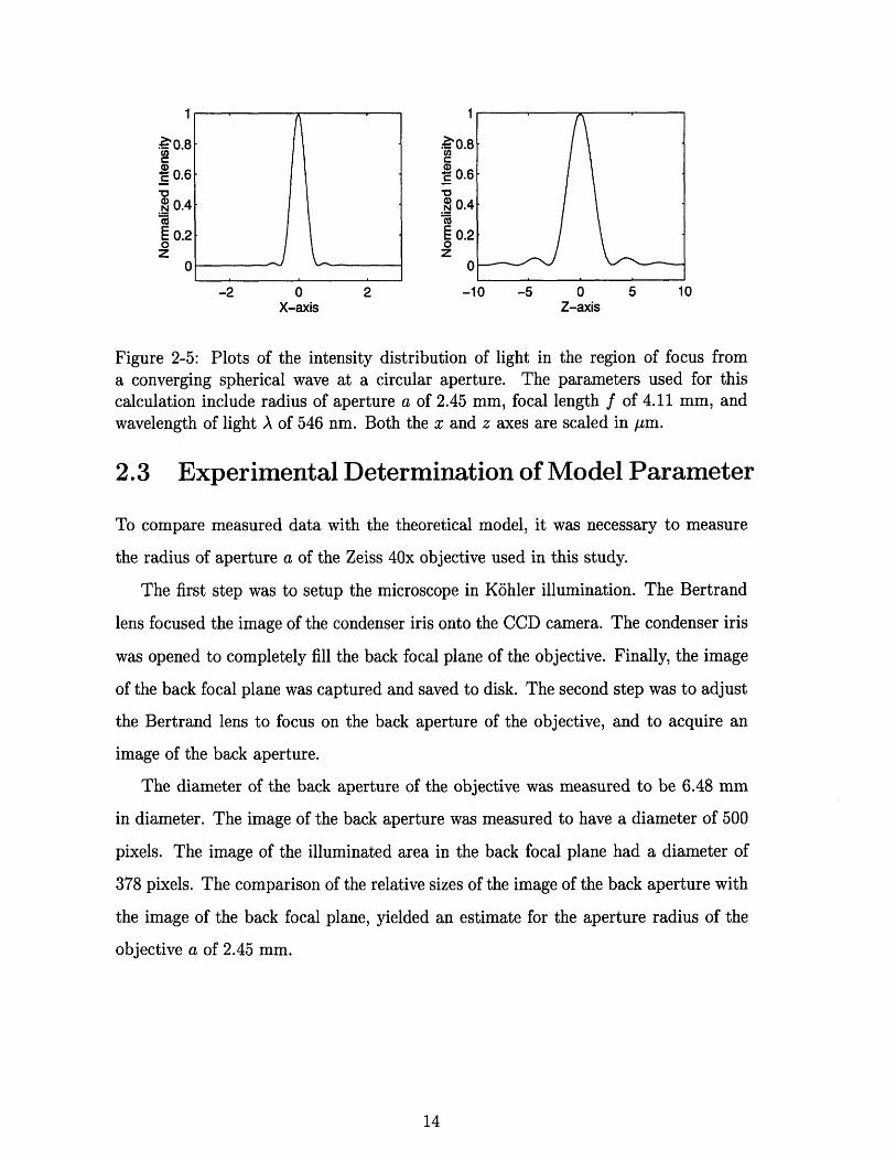
Figure 2-5 illustrates the intensity pattern along the x and z axes. The plot is
scaled for the parameters of our Zeiss 40x water immersion objective with a 1.95 mm
working distance and NA of 0.75 used in this study. The information about the focal
length f was provided from the manufacturer [8], however, the radius of aperture a
was not.
i0.8C
_ 0.6
. 0.4
, 0.200
-2 0 2 -10 -5 0 5 10X-axis Z-axis
Figure 2-5: Plots of the intensity distribution of light in the region of focus froma converging spherical wave at a circular aperture. The parameters used for thiscalculation include radius of aperture a of 2.45 mm, focal length f of 4.11 mm, andwavelength of light A of 546 nm. Both the x and z axes are scaled in /.m.
2.3 Experimental Determination of Model Parameter
To compare measured data with the theoretical model, it was necessary to measure
the radius of aperture a of the Zeiss 40x objective used in this study.
The first step was to setup the microscope in Kahler illumination. The Bertrand
lens focused the image of the condenser iris onto the CCD camera. The condenser iris
was opened to completely fill the back focal plane of the objective. Finally, the image
of the back focal plane was captured and saved to disk. The second step was to adjust
the Bertrand lens to focus on the back aperture of the objective, and to acquire an
image of the back aperture.
The diameter of the back aperture of the objective was measured to be 6.48 mm
in diameter. The image of the back aperture was measured to have a diameter of 500
pixels. The image of the illuminated area in the back focal plane had a diameter of
378 pixels. The comparison of the relative sizes of the image of the back aperture with
the image of the back focal plane, yielded an estimate for the aperture radius of the
objective a of 2.45 mm.
Chapter 3
Methods
3.1 Measuring the PSF
3.1.1 Experimental Setup: Overview
The imaging system described in this chapter consists of a Zeiss Axioplan light micro-
scope using a Zeiss 40x water immersion objective with a 1.95 mm working distance
and numerical aperture (NA) of 0.75. This system is fitted with a CCD camera and
a video digitizer card (Photometrics) installed on a personal computer. The images
are sampled by the camera and stored to disk. The specimen stage is connected to a
stepper motor, and its position is automatically controlled by the computer. The sys-
tem is capable of automatically taking a volume measurement of a target by recording
images over a range of planes of focus within the specimen.
3.1.2 Sampling the Image
Whenever one uses a CCD camera or any other sampling device, care must be taken
that the samples occur at a rate to avoid aliasing, and to insure that the sampled
signal is a good representation of the actual signal. To do this, we need to investigate
the spatial frequencies that need to be sampled by our CCD.
The resolution of a microscope is limited by the NA of the objective and the
wavelength of light used to generate the image. The spatial frequency at which the
contrast in the microscope image approaches zero is called the cutoff frequency. For
our system, the cutoff spatial frequency is fc = 2NA 2.77/m-1 [9].
The field of view of the CCD camera is 382x576 pixels. Each pixel is 23 pm
square. To avoid aliasing, the image plane must be sampled at a spatial frequency
greater than twice the cutoff frequency. At a magnification of 400x, each pixel in the
image plane corresponds to a square of length I = 0.0575 pm in the specimen plane.
This rate corresponds to a sampling frequency of f, = 17.4 pm- 1 which is well above
the Nyquist criteria. At this rate, aliasing is not a problem.
Not only is it important to avoid aliasing within the plane of each two dimensional
image (in the x and y directions), but since we are dealing with three-dimensional
volumes of data, it is also important to sample at an appropriate rate in the z direction.
The depth of focus for our system is given by:
Az = A
4n(1 - 1 - ( )2
where the wavelength of light, A is 546 nm, the numerical aperture of the objective,
NA is 0.75, and index of refraction of water, n is 1.333 [10]. The depth of focus is
about 0.6 pm. We sampled at increments of 0.27 pm in the z direction.
3.1.3 Two-Dimensional Step Target
To measure the PSF, it is necessary to choose an appropriate target or input with
which to characterize the system. The first major approach is to measure a step
response by blocking half of the field of view in brightfield illumination. The derivative
of the step response yields the line spread function (LSF) . Others have asserted that
the LSF is equivalent to the PSF if the PSF of the lens is circularly symmetric [10].
However, the LSF is actually composed of a series of overlapping PSFs arranged in a
straight line. Therefore, the LSF is at best only an approximation to the PSF.
Initial experiments involving the measurement of the step response involved the
imaging of an optical slit (Ealing #43-5982) placed in the specimen plane of the
microscope. At high magnification, imperfections in the slit were readily apparent.
The slit failed to provide a clean straight edge. Later experiments used a common
razor blade in place of an optical slit. The razor blade had two major advantages
over the optical slit for this application. The first advantage is that its cost is several
orders of magnitude less than that of the optical slit. The second advantage is that
the razor blade has a much cleaner and more straight edge from which to obtain a
quality image.
3.1.4 Three-Dimensional Point Target
The second major approach to measuring the PSF is to build a target consisting of
small microspheres dispersed in a gel or other mounting medium. This approach leads
to a direct measurement of the PSF. Unfortunately, microspheres are not trivial to
use. They must be small with respect to the resolution of the microscope in order to
simulate an impulse in space. Therefore, by their nature, they are difficult to visualize
in the microscope. Both 0.2 pm and 0.5 jm diameter microspheres manufactured
by Polysciences Inc. were chosen to approximate an impulse. When performing an
experiment, it is vital that one can differentiate a microsphere from a piece of dust or
grime corrupting the optical path. The solution to this problem is to use fluorescent
microspheres. The target can then be viewed in fluorescence microscopy to find a
microsphere and to be certain that one was actually viewing a microsphere, assuming
that typical dust and grime do not fluoresce. After focusing on a microsphere in
fluorescence microscopy, one can measure the fluorescence PSF. One can also switch to
brightfield microscopy while keeping the same bead in focus to measure the brightfield
PSF.
Microspheres in Gel
The 40x objective used in this project is not corrected for use with a coverslip. There-
fore, in order to accurately measure the PSF, it is necessary to build targets that do
not have a coverslip. At the same time, the microspheres need to be held in a fixed
position while they are being imaged. Therefore, a dispersion of microspheres is
immobilized in a gel.
In initial experiments the targets thus constructed did not work effectively. The use
of a water immersion lens requires a water droplet to be situated immediately between
the objective and the target. This arrangement is very useful for most applications
involving biological samples. Unfortunately, due to a difference in osmotic pressure
between the water droplet and the gel, solvent transport occurs, and the gel swells
causing significant motion of the microsphere. Therefore, the gel initially failed to
hold the microsphere in a fixed location.
To alleviate this dilemma, the osmolarity of the solutions involved in constructing
the targets is controlled more carefully. Instead of making the gel as a mixture of
water and gelatin, the gel is made as a mix of modified artificial endolymph (MAE)
solution and gelatin. The rationale for the choice of MAE is that MAE is a commonly
used solution in our laboratory, and its presence increases the osmolarity and controls
the pH of the gel. Instead of using a water droplet between the objective and the gel,
a droplet of MAE is used instead. Therefore, both the osmolarity of the gel and the
droplet are determined by the MAE solution.
MAE contains (in mmol/L): NaCl (1.5), KC1 (174), Hepes (5), dextrose (5), and
sucrose (50). The pH of MAE is adjusted to 7.3. The recipe for the construction of
gelatin targets is as follows. One gram of research grade gelatin (Sigma) is mixed into
40 mL of MAE, and heated until dissolved. To this mixture, microspheres, originally
provided in a dispersion of 2.5% solids from the vendor, are added at a concentration
of 5 1tL per 10 mL MAE gelatin mixture. From this, 30 pL of the resulting solution
is placed inside a trough created by an o-ring glued to a microscope slide. The
preparation is sealed in a petri dish, and stored in a refrigerator to set overnight.
Microspheres in Mount-Quick
Several targets were constructed with a coverslip to evaluate the significance of spher-
ical aberration caused by incorrect coverslip thickness. These targets are construc-
ted by first diluting the microsphere concentration by mixing 10 pL of microsphere
solution from the vendor with 10 mL of water. Next, 10 pL of the resulting solu-
tion is mixed with 3 drops of Mount-Quick (Electron Microscopy Sciences) mounting
medium. Thirty pL of the final mixture are transferred to a slide, covered with a
coverslip, and let set overnight. Lastly, the square coverslip/slide perimeter is coated
with clear nail polish to strengthen and protect the target.
3.2 Data Analysis
3.2.1 Two-Point Correction
Raw images from the CCD camera are processed by two-point correction to reduce
fixed pattern noise, and to improve image quality [3]. There are two types of fixed
pattern noise-multiplicative and additive noise. For example, if the CCD camera
takes a picture while the shutter is closed, it will not measure an even field of zero
intensity across the CCD. The thermal production of hole-electron pairs will cause
charge to be deposited across the CCD. The intensity of this so-called dark image
(of additive noise) will depend on the exposure time used to take the picture. If a
picture of empty space in the specimen plane is taken (with the shutter open), one
would not observe an even intensity measurement across the CCD. Dust and other
particles that contaminate the optical path can be modeled as having a multiplicative
light absorbance. The intensity pattern measured at different points of observation
across the image plane will be scaled differently (from the absorbing effect of dust),
but fortunately this pattern is also consistent and correctable. For every set of PSF
measurements, both a light background image as well as a dark image (taken with the
closed shutter) is recorded. These measurements are then used to reduce the fixed
pattern noise:
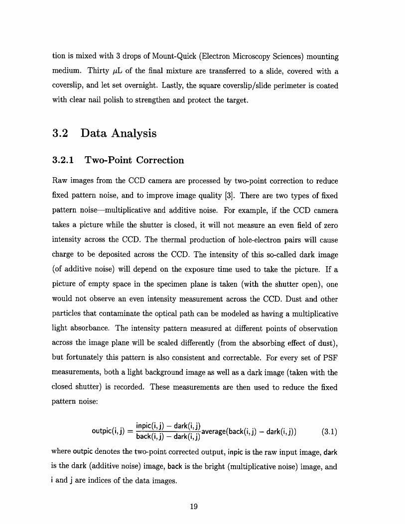
Sinpic(i,j) - dark(i,j) . ..outpic(i,j) = p - average(back(i,j) - dark(i,j)) (3.1)back(ij) - dark(ij)where outpic denotes the two-point corrected output, inpic is the raw input image, dark
is the dark (additive noise) image, back is the bright (multiplicative noise) image, and
i and j are indices of the data images.
3.2.2 Normalization and Statistics
It is important to consistently normalize the data so that PSF measurements in bright-
field microscopy can be compared to PSF measurements in fluorescence microscopy.
Additionally, data taken from the same microsphere at different times will have a
slightly different DC-offset, and it is important to be able to compare these kinds of
results in a systematic way. The first step is to define a shifting algorithm so that
the background, or apparently empty, region of the image can be defined to have an
intensity of zero. This facilitates the comparison of the change in intensity caused by
the target.
From each volume measurement, the global extremum is found and a frame of
reference is defined with this extremum at the origin. Note that the mapping of the
extremum of each waveform to the origin does not correct for subpixel shifts in the
waveform. The x, y and z axes are aligned with the original microscope axes. The
intensity values along the new x and z axes are used to calculate statistics about the
given volume of data. In general, the intensity values along the x axis at the edge
of each image always consists of an apparently empty region. Therefore, the average
of the 21 pixel values at each edge of the x axis, farthest away from the effect of
the microsphere, is defined as the baseline pixel value. This baseline pixel value is
subtracted from the intensity data along both x and z axes, yielding a set of data with
the background intensity defined as zero.
For the purpose of statistical analysis, it is important to create a consistent means
of defining the width of the PSF. From the shifted dataset, it is intuitive to define the
region of the PSF where the intensity values along the x axis are within one half of its
extremum to be the width of the PSF. This definition when applied to the intensity
values along the z axis yields the height of the PSF.
3.3 Index of Refraction of Gel
A coverslip is a source of spherical aberration if used in conjunction with an objective
that is not corrected for use with one. In Figure 3-1, the light emerging from a point
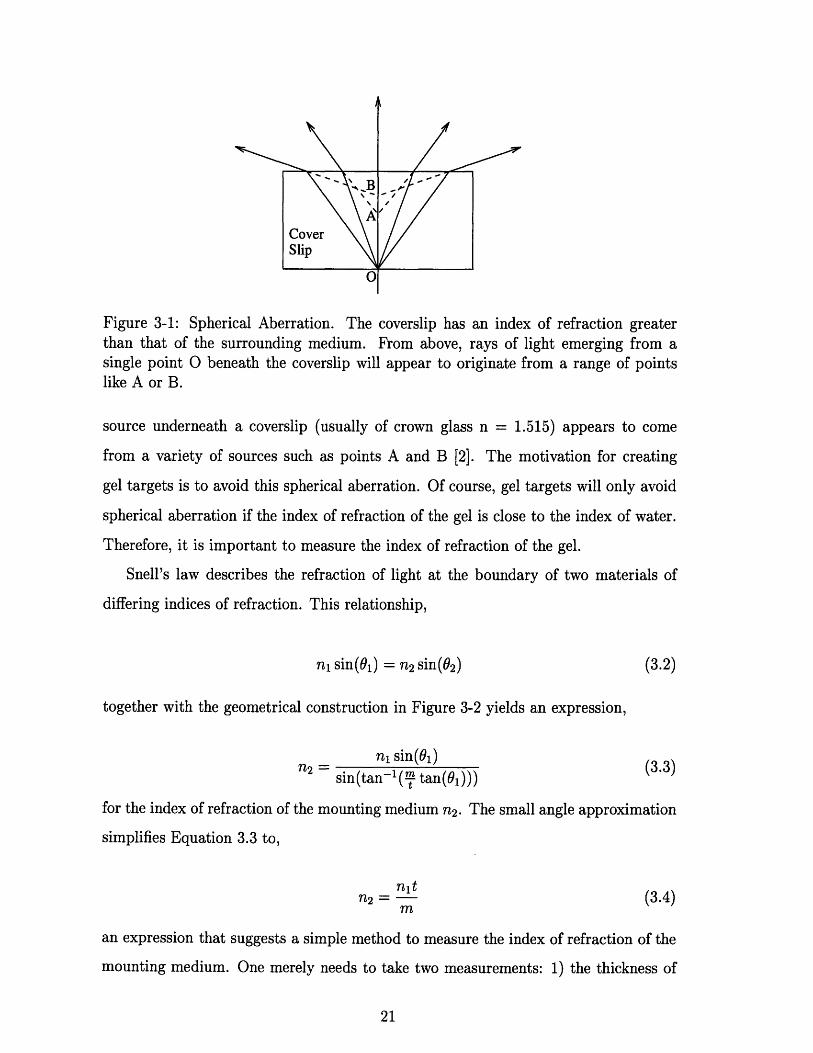
Figure 3-1: Spherical Aberration. The coverslip has an index of refraction greaterthan that of the surrounding medium. From above, rays of light emerging from asingle point O beneath the coverslip will appear to originate from a range of pointslike A or B.
source underneath a coverslip (usually of crown glass n = 1.515) appears to come
from a variety of sources such as points A and B [2]. The motivation for creating
gel targets is to avoid this spherical aberration. Of course, gel targets will only avoid
spherical aberration if the index of refraction of the gel is close to the index of water.
Therefore, it is important to measure the index of refraction of the gel.
Snell's law describes the refraction of light at the boundary of two materials of
differing indices of refraction. This relationship,
nl sin(01) = n2 sin(l 2 ) (3.2)
together with the geometrical construction in Figure 3-2 yields an expression,
ni sin(01)n2 = (3.3)sin(tan-(1( tan(01)))
for the index of refraction of the mounting medium n2. The small angle approximation
simplifies Equation 3.3 to,
n i tn2 = (3.4)
an expression that suggests a simple method to measure the index of refraction of the
mounting medium. One merely needs to take two measurements: 1) the thickness of
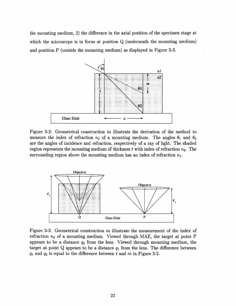
the mounting medium, 2) the difference in the axial position of the specimen stage at
which the microscope is in focus at position Q (underneath the mounting medium)
and position P (outside the mounting medium) as displayed in Figure 3-3.
Figure 3-2: Geometrical construction to illustrate the derivation of the method tomeasure the index of refraction n2 of a mounting medium. The angles 01 and 02are the angles of incidence and refraction, respectively of a ray of light. The shadedregion represents the mounting medium of thickness t with index of refraction n2. Thesurrounding region above the mounting medium has an index of refraction nl.
Objective
Figure 3-3: Geometrical construction to illustrate the measurement of the index ofrefraction n2 of a mounting medium. Viewed through MAE, the target at point Pappears to be a distance q2 from the lens. Viewed through mounting medium, thetarget at point Q appears to be a distance ql from the lens. The difference betweenql and q2 is equal to the difference between t and m in Figure 3-2.
Chapter 4
Results
4.1 Repeatability of Measurements
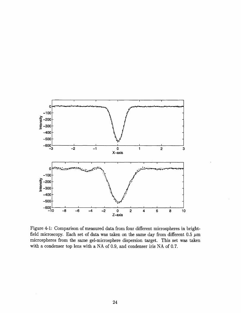
Figure 4-1 shows a set of measurements in brightfield illumination from four different
0.5 /1 m microspheres. The data was taken in a successive series of experiments on the
same day. The values of the waveforms, when aligned by their peaks are generally
within 20% of each other. The ratio of the energy in the waveforms with the energy
in their differences are compared for several different cases. For measurements taken
on the same day with the same microsphere, the ratios are 18dB, and 16dB for the x
and z directions respectively. For measurements taken on the same day with different
microspheres, the ratios are 22dB, and 14dB for x and z directions respectively. For
measurements taken on different days with different microspheres, the ratios are 19dB
and 17dB respectively.
In Figure 4-1 between 4 and 10 jtm above the minimum, the waveform is primarily
flat. However, between 4 and 10 pm below the minimum, each waveform displays a
consistent damped ringing. This ringing is visible in most PSF measurements. In
Figures 4-2 and 4-3, there exists a fairly consistent checkerboard pattern beneath the
dark minimum in brightfield (or bright maximum in fluorescence) in each image. The
corresponding intensity plots also exhibit a ringing behavior along the negative z axis.
Z-
X-axis
a,
)Z-axis
Figure 4-1: Comparison of measured data from four different microspheres in bright-field microscopy. Each set of data was taken on the same day from different 0.5 1/mmicrospheres from the same gel-microsphere dispersion target. This set was takenwith a condenser top lens with a NA of 0.9, and condenser iris NA of 0.7.
4.2 Fluorescence Microscopy
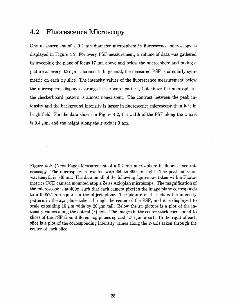
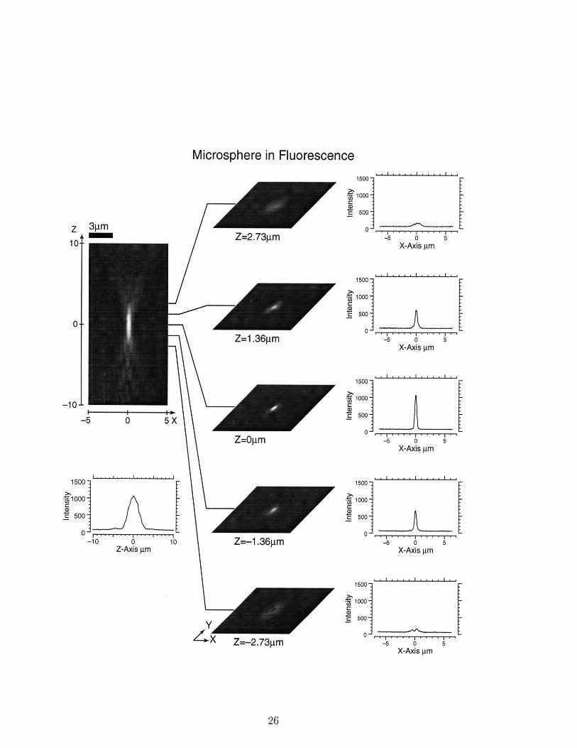
One measurement of a 0.2 /m diameter microsphere in fluorescence microscopy is
displayed in Figure 4-2. For every PSF measurement, a volume of data was gathered
by sweeping the plane of focus 17 pm above and below the microsphere and taking a
picture at every 0.27 pm increment. In general, the measured PSF is circularly sym-
metric on each xy slice. The intensity values of the fluorescence measurement below
the microsphere display a strong checkerboard pattern, but above the microsphere,
the checkerboard pattern is almost nonexistent. The contrast between the peak in-
tensity and the background intensity is larger in fluorescence microscopy than it is in
brightfield. For the data shown in Figure 4-2, the width of the PSF along the x axis
is 0.4 pm, and the height along the z axis is 3 pm.
Figure 4-2: (Next Page) Measurement of a 0.2 pm microsphere in fluorescence mi-croscopy. The microsphere is excited with 450 to 490 nm light. The peak emissionwavelength is 540 nm. The data on all of the following figures are taken with a Photo-metrics CCD camera mounted atop a Zeiss Axioplan microscope. The magnification ofthe microscope is at 400x, such that each camera pixel in the image plane correspondsto a 0.0575 pm square in the object plane. The picture on the left is the intensitypattern in the x,z plane taken through the center of the PSF, and it is displayed toscale extending 10 pm wide by 20 pm tall. Below the xz picture is a plot of the in-tensity values along the optical (z) axis. The images in the center stack correspond toslices of the PSF from different xy planes spaced 1.36 pm apart. To the right of eachslice is a plot of the corresponding intensity values along the x-axis taken through thecenter of each slice.
Microsphere in Fluorescence1500 -51000
t-
C 500 V
0-5 0 5
X-Axis Im
15001
1000
S500
0-5 0 5
X-Axis gm
15001
0J-5 0 5
X-Axis gm
1500
1000 A500 -
0L-5 0 5
X-Axis gLm
15001
1000
500 F0-
-5 0 5X-Axis gm
Z
101
-10
150(
•55100(
C 50(
(
Z--X Z=-2.731gm
4.3 Brightfield Microscopy
4.3.1 Effect of Microsphere Size
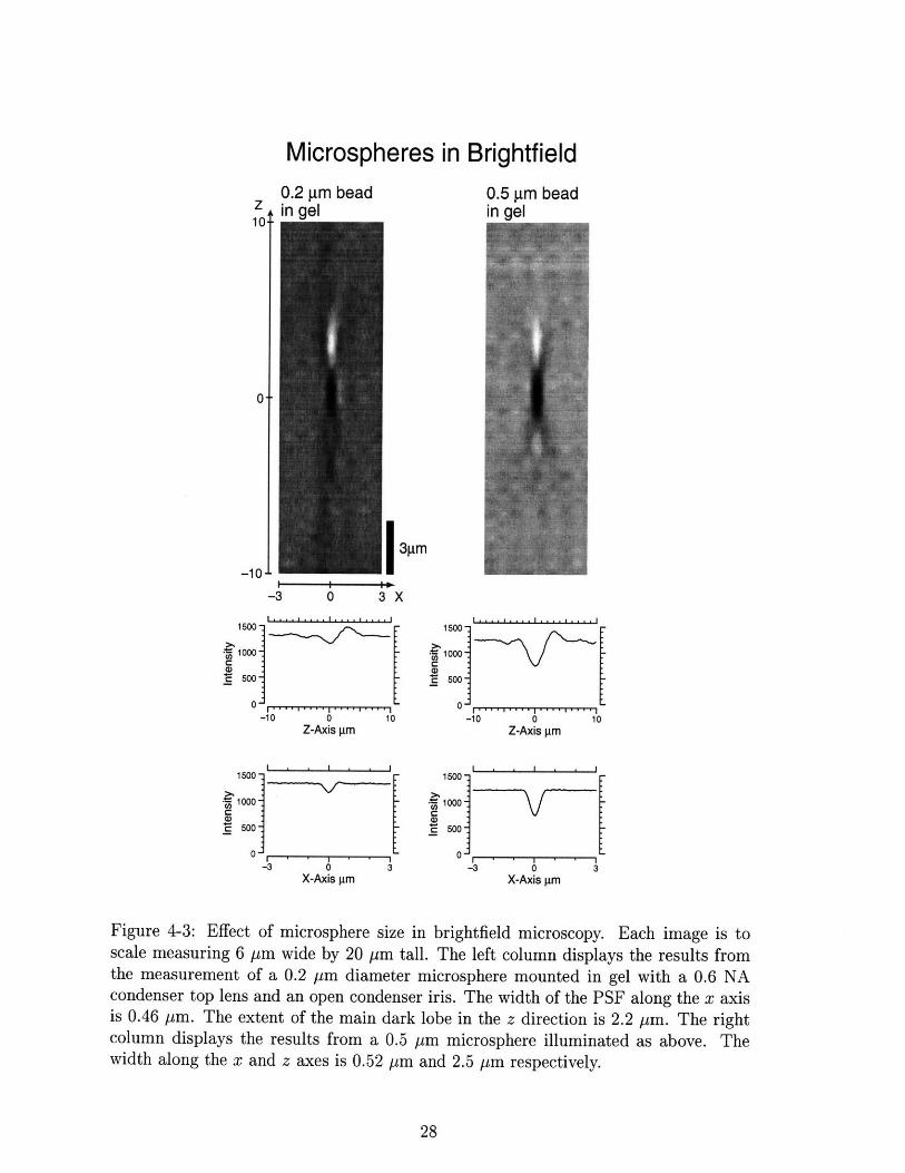
Figure 4-3 compares results from two sets of measurements of different sized micro-
spheres taken in brightfield microscopy. The images and the data plotted beneath
each image are the two-point corrected output from the fixed pattern noise reduction
algorithm described in Chapter 3. Unlike the intensity plots in Figure 4-1, all of the
intensity plots in z for data in Figure 4-3 exhibit a maximum corresponding to a bright
spot. Note that the data in Figure 4-1 was taken with a different condenser top lens.
The measurements of the 0.2 pm microsphere and the 0.5 pm microsphere in gel
are very similar. However, the measurement from the 0.5 pm microsphere is slightly
larger in size, and greater in contrast. Notice the contrast between the dark spot
intensity and the background intensity for the 0.2 pm microsphere is less than half the
contrast for the 0.5 pm microsphere.
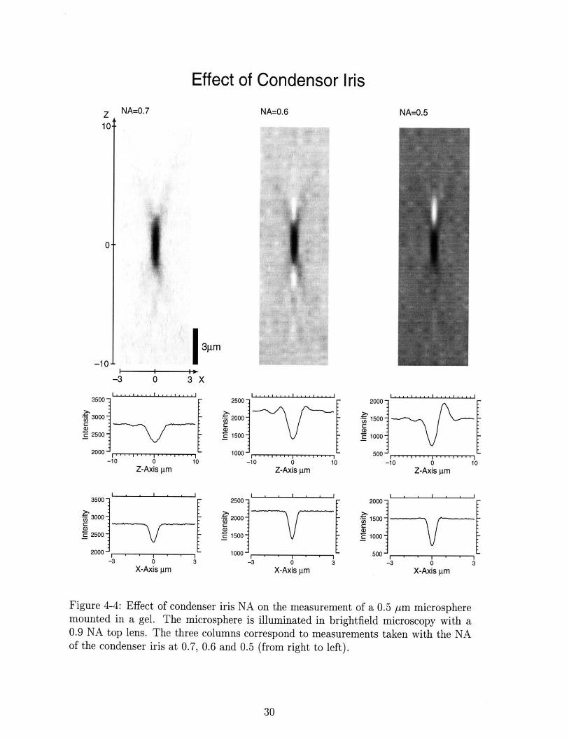
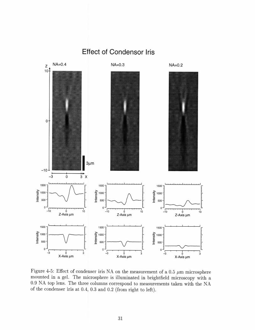
4.3.2 Effect of Condenser Iris NA
Figures 4-4 and 4-5 show results from the measurement of a 0.5 pm microsphere
mounted in a gel. The microsphere is illuminated in brightfield microscopy. Unlike
the measurements in Figure 4-3, this set is taken with a condenser stage top lens with a
NA of 0.9. The data from the 0.5 pm microsphere with the 0.6 NA top lens (Figure 4-
3) is similar to the the data taken with the 0.9 NA top lens and the condenser iris set
at an effective NA of 0.6 (Figure 4-4). The condenser iris is adjusted to illuminate the
microsphere with an angular spectrum of light ranging in an effective NA from 0.7 to
0.2. Notice that as the NA is decreased, the measurement radically changes.
When the condenser iris NA is 0.7, which almost completely fills the NA of the
objective lens, the resulting measurement very closely resembles the measurement for
the 0.2 pm microsphere in fluorescence except that it is slightly larger and in reverse
video. As the effective NA of the condenser iris is reduced to 0.6 as shown in Figure 4-
4, the main lobe in the z direction shrinks. Bright sidelobes begin to form. As the NA
Microspheres in Brightfield0.2 pm beadin ael
0.5 pLm bead
I 3jmI I I
-3 0 3 X
Z-Axis gLm Z-Axis gIm
1500
· 1000F
E 500 -
0-3 0 3
X-Axis gm X-Axis gLm
Figure 4-3: Effect of microsphere size in brightfield microscopy. Each image is toscale measuring 6 pm wide by 20 pm tall. The left column displays the results fromthe measurement of a 0.2 pm diameter microsphere mounted in gel with a 0.6 NAcondenser top lens and an open condenser iris. The width of the PSF along the x axisis 0.46 pm. The extent of the main dark lobe in the z direction is 2.2 /tm. The rightcolumn displays the results from a 0.5 pm microsphere illuminated as above. Thewidth along the x and z axes is 0.52 pm and 2.5 pm respectively.
z10
0.
-10
w
-
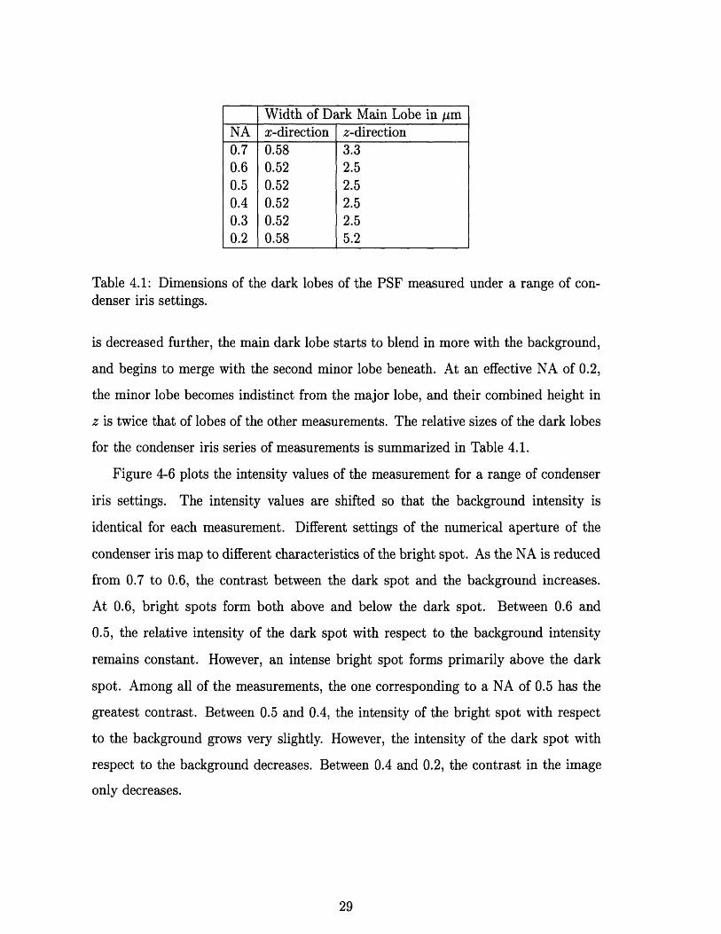
Table 4.1: Dimensions of the dark lobes of the PSF measured under a range of con-denser iris settings.
is decreased further, the main dark lobe starts to blend in more with the background,
and begins to merge with the second minor lobe beneath. At an effective NA of 0.2,
the minor lobe becomes indistinct from the major lobe, and their combined height in
z is twice that of lobes of the other measurements. The relative sizes of the dark lobes
for the condenser iris series of measurements is summarized in Table 4.1.
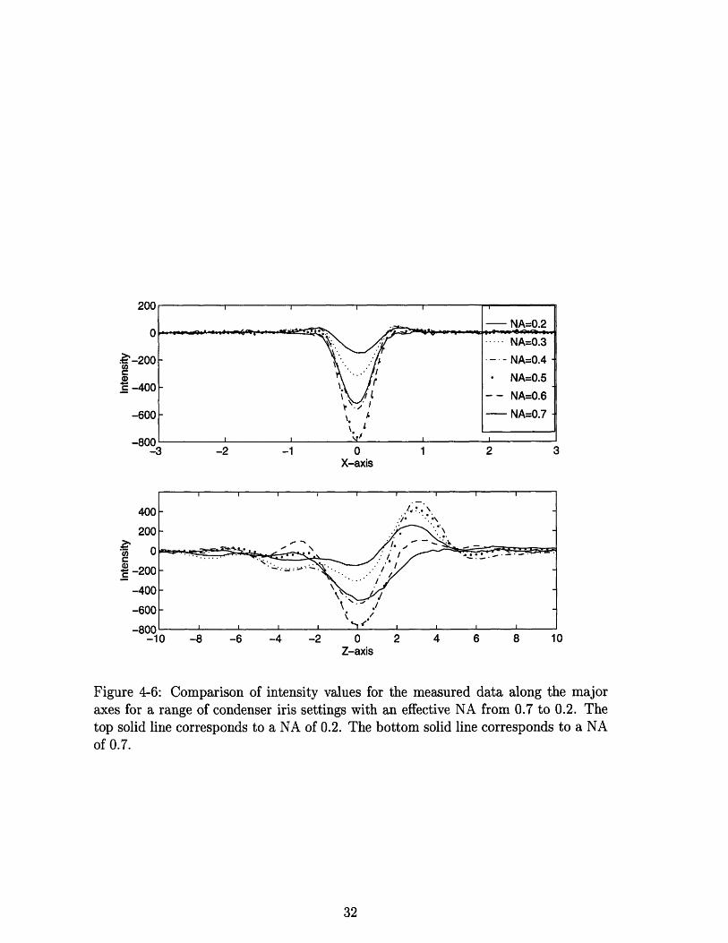
Figure 4-6 plots the intensity values of the measurement for a range of condenser
iris settings. The intensity values are shifted so that the background intensity is
identical for each measurement. Different settings of the numerical aperture of the
condenser iris map to different characteristics of the bright spot. As the NA is reduced
from 0.7 to 0.6, the contrast between the dark spot and the background increases.
At 0.6, bright spots form both above and below the dark spot. Between 0.6 and
0.5, the relative intensity of the dark spot with respect to the background intensity
remains constant. However, an intense bright spot forms primarily above the dark
spot. Among all of the measurements, the one corresponding to a NA of 0.5 has the
greatest contrast. Between 0.5 and 0.4, the intensity of the bright spot with respect
to the background grows very slightly. However, the intensity of the dark spot with
respect to the background decreases. Between 0.4 and 0.2, the contrast in the image
only decreases.
Width of Dark Main Lobe in imNA x-direction z-direction0.7 0.58 3.30.6 0.52 2.50.5 0.52 2.50.4 0.52 2.50.3 0.52 2.50.2 0.58 5.2
Effect of Condensor IrisNA=0.6
I 3m-3 0 3 X
3500 .
3000
c 2500
2000-10 0 10
Z-Axis gLm
35001
3000 7
c 2500
2000 --3 0 3g
X-Axis jim
25007
2000
1500
1000-10 0 10
Z-Axis gm
2500-
CO 20001
) 1500
15001 L_I ' ' I I , I-3 0 3
X-Axis gm
20007
*,15001C
10001
500
-10 0 10Z-Axis jLm
I . . I , , I2000-
S1500
E 1000
500 "' ._ ._-3 0 3
X-Axis gm
Figure 4-4: Effect of condenser iris NA on the measurement of a 0.5 pm microspheremounted in a gel. The microsphere is illuminated in brightfield microscopy with a0.9 NA top lens. The three columns correspond to measurements taken with the NAof the condenser iris at 0.7, 0.6 and 0.5 (from right to left).
Z NA=0.7
10:
NA=0.5
Effect of Condensor Iris
I 34mI I Na
-3 0 3 X
1500
10001
E 500
0"-10 0 10
Z-Axis pm
I ' ' I " ' I1500
.1000-
c 500 -
-3 0 3X-Axis pm
1500
C 500
0
-10 0 10Z-Axis pm
I , , I , , I1500-
1000-
c 500
0-3 0 3
X-Axis pm
1500
O 10001C 1
E 50010-10 0 10
Z-Axis gm
I , I , , I15007
10007
U)5001
0-
-3 0 3X-Axis pm
Figure 4-5: Effect of condenser iris NA on the measurement of a 0.5 um microspheremounted in a gel. The microsphere is illuminated in brightfield microscopy with a0.9 NA top lens. The three columns correspond to measurements taken with the NAof the condenser iris at 0.4, 0.3 and 0.2 (from right to left).
z NA=0.4 NA=0.3 NA=0.210
0*
-10-
10
•
-
200
0
-200
-400
-600
-_,00
Co0)C
-3 -2 -1 0 1 2 3X-axis
DZ-axis
Figure 4-6: Comparison of intensity values for the measured data along the majoraxes for a range of condenser iris settings with an effective NA from 0.7 to 0.2. Thetop solid line corresponds to a NA of 0.2. The bottom solid line corresponds to a NAof 0.7.
NA=0.2
.... NA=0.3
- - NA=0.4 -
* NA=0.5
-- NA=0.6
- NA=0.7
A'[
I I _/ I I
_· · · ·
4.4 Effect of Aberrations
4.4.1 Chromatic Aberration
A previous study that attempted to measure the PSF report results that differ from
those shown here [4]. One possible explanation for this discrepancy could be the effect
of chromatic or spherical aberrations.
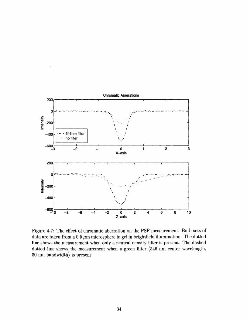
Chromatic aberrations occur as a result of the fact that the index of refraction in
glass is a function of wavelength. Figure 4-7 shows the effect of chromatic aberration
on a PSF measurement in brightfield. The data for this plot have been shifted to
equalize the background intensity. Notice that when no green filter is present, the
waveform has about one third of the contrast and is almost twice as tall in z.
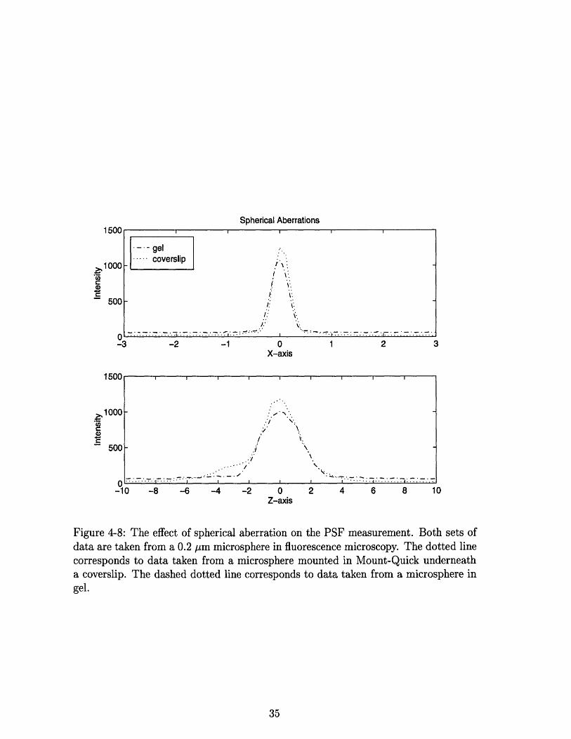
4.4.2 Spherical Aberration
The effect of a coverslip in fluorescence microscopy is shown in Figure 4-8. Data
collected for a 0.2 /m diameter microsphere mounted in Mount-Quick (Electron Mi-
croscopy Sciences) with a coverslip is compared to the results for a 0.2 /am microsphere
mounted in a gel, also in fluorescence microscopy. The major difference between these
two measurements is that the target with the coverslip has a bump in the intensity
pattern between -4 and -2 1am along the z axis.
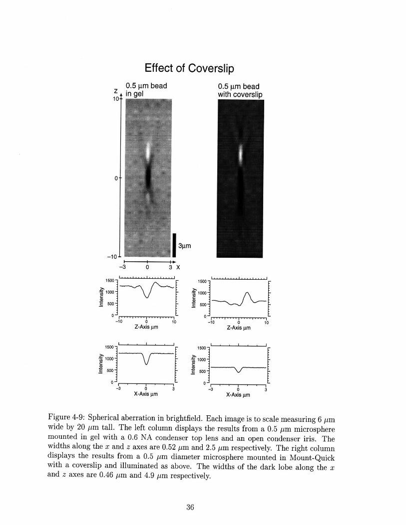
In brightfield illumination, the effect of a coverslip is to increase the intensity of
the bright spot, and to extend the dark lobe in z as shown in Figure 4-9. The shape
of the main dark lobe has a camel-back hump-similar to those measurements taken
at low condenser NA (Figure 4-5). The main dark lobe and the minor dark lobe
beneath have both been extended in z such that they have ceased to be distinct from
one another. Also, the bright spot above the microsphere has a greater contrast with
respect to the background than the dark spot-again, this phenomenon is similar to
those measurements taken at low condenser NA.
Chromatic Aberrations
0X-axis
-8 -6 -4 -2 0Z-axis
2 4 6 8
Figure 4-7: The effect of chromatic aberration on the PSF measurement. Both sets ofdata are taken from a 0.5 im microsphere in gel in brightfield illumination. The dottedline shows the measurement when only a neutral density filter is present. The dasheddotted line shows the measurement when a green filter (546 nm center wavelength,30 nm bandwidth) is present.
LVu
0
g -200
-400
00
. ;
\ i
-- - 546nm filter \ I..... no filter \ /
- 3UUV-3
200
0
-200
-400
-600-1
I I I I I I I I I
I.
..
· · ·
1
-
0
" '. ;,:·~';;.~·T.'. 5r ·........ · r'~
'''··
I I I I I I I I I
Spherical Aberrations
3 -2 -1 0 1 2X-axis
.1
. 4 .. .....! \'. '''
-8 -6 -4 -2 0Z-axis
2 4 6 8 10
Figure 4-8: The effect of spherical aberration on the PSF measurement. Both sets ofdata are taken from a 0.2 pm microsphere in fluorescence microscopy. The dotted linecorresponds to data taken from a microsphere mounted in Mount-Quick underneatha coverslip. The dashed dotted line corresponds to data taken from a microsphere ingel.
1500
I nnr
..gel.coverslip
.7.-I" (..
., .
i, k
5bU
1500
1 nnrI VUi.J
5bU
r-10
IVVu
Effect of Coverslip0.5 gm bead
10
-10
0.5 gm beadwith coverslip
I mI I 3X
-3 0 3 X
1500
C 500
-10 0 10Z-Axis gLm
0 I ' , ' I1500,
C 500-
0--3 0 3
X-Axis gLm
I.,,I,,!..I .1 .. . I1500
000
-10 0 10Z-Axis gm
I I1500
1000
C 500a, r
0
-3 0 3X-Axis jim
Figure 4-9: Spherical aberration in brightfield. Each image is to scale measuring 6 pmwide by 20 pm tall. The left column displays the results from a 0.5 Am microspheremounted in gel with a 0.6 NA condenser top lens and an open condenser iris. Thewidths along the x and z axes are 0.52 pm and 2.5 pm respectively. The right columndisplays the results from a 0.5 pm diameter microsphere mounted in Mount-Quickwith a coverslip and illuminated as above. The widths of the dark lobe along the xand z axes are 0.46 pm and 4.9 pm respectively.
z
-
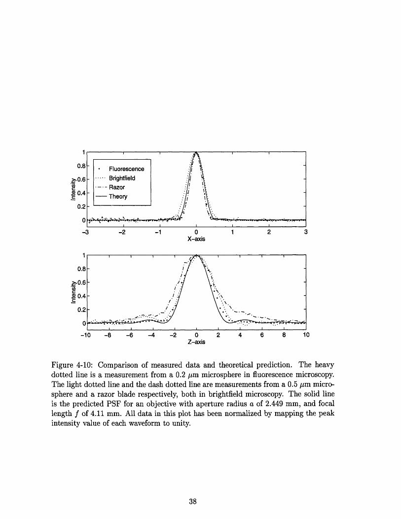
4.5 Comparison of Results to Theory
Figure 4-10 plots four sets of data: 1) the normalized intensity of the PSF measured
from a 0.2 Im microsphere in fluorescence, 2) the normalized intensity of the PSF
measured from a 0.5 jm microsphere in brightfield with a condenser iris at an ef-
fective NA of 0.7, 3) the normalized intensity of the razor blade line spread function
measurement (LSF), and 4) the normalized intensity of the theoretical PSF.
The waveforms are normalized by mapping the extremum to one, and mapping
the average value of the background intensity to zero as described in Chapter 3. As a
result, the brightfield data has been flipped about the horizontal axis so that the peak
is positive with respect to the background. This facilitates the comparison of PSF
measurements from different types of microscopy.
According to Equation 2.6, the PSF in focus on the xy plane should have a width
of about 0.52 jm. In fluorescence, and from razor blade measurements, the data
indicates a PSF width of about 0.40 jim. In brightfield, the measured data indicates a
PSF width of about 0.58 jm. Equation 2.7 predicts the PSF along the optical z axis
to extend about 2.45 jm. The measured data indicates 3 jm for fluorescence, 3.3 pm
for brightfield, and 3.8 jim for the LSF.
Notice that the LSF along the z axis is greater in magnitude than the other meas-
urements within 8 pm of the peak. The LSF obtained from the razor blade data was
expected to be an approximation of the PSF. More precisely, the LSF is the summa-
tion of a series of overlapping PSFs arranged in a straight line. An xz slice of a LSF
situated along the y axis will consist of a contribution from the PSF in the plane plus
the contribution from a series of PSFs successively further from that plane. Each
contribution to the LSF is identical to one of the xz slices in the PSF. The sum of all
of the xz slices in the PSF will therefore yield the LSF. Figure 4-11 compares the LSF
to the summation of the fluorescence measurement. The summation was acquired by
adding the intensity values along every line in the y direction of the original two-point
corrected volume of data.
The values of the summation of the fluorescence PSF measurement are slightly
0.8
>,0.6
1 0.4
0.2
0
-3 -2 -1 0 1 2 3X-axis
-10 -8 -6 -4 -2 0 2 4 6 8 10Z-axis
Figure 4-10: Comparison of measured data and theoretical prediction. The heavydotted line is a measurement from a 0.2 pm microsphere in fluorescence microscopy.The light dotted line and the dash dotted line are measurements from a 0.5 Pm micro-sphere and a razor blade respectively, both in brightfield microscopy. The solid lineis the predicted PSF for an objective with aperture radius a of 2.449 mm, and focallength f of 4.11 mm. All data in this plot has been normalized by mapping the peakintensity value of each waveform to unity.
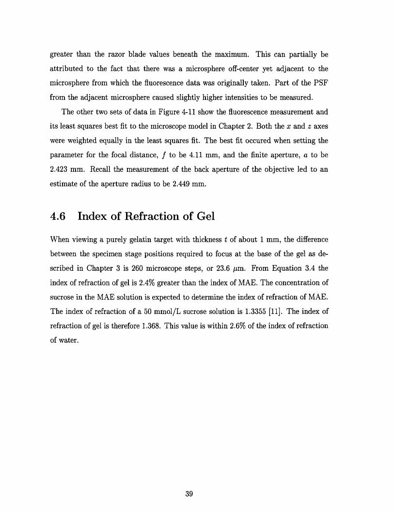
greater than the razor blade values beneath the maximum. This can partially be
attributed to the fact that there was a microsphere off-center yet adjacent to the
microsphere from which the fluorescence data was originally taken. Part of the PSF
from the adjacent microsphere caused slightly higher intensities to be measured.
The other two sets of data in Figure 4-11 show the fluorescence measurement and
its least squares best fit to the microscope model in Chapter 2. Both the x and z axes
were weighted equally in the least squares fit. The best fit occured when setting the
parameter for the focal distance, f to be 4.11 mm, and the finite aperture, a to be
2.423 mm. Recall the measurement of the back aperture of the objective led to an
estimate of the aperture radius to be 2.449 mm.
4.6 Index of Refraction of Gel
When viewing a purely gelatin target with thickness t of about 1 mm, the difference
between the specimen stage positions required to focus at the base of the gel as de-
scribed in Chapter 3 is 260 microscope steps, or 23.6 pm. From Equation 3.4 the
index of refraction of gel is 2.4% greater than the index of MAE. The concentration of
sucrose in the MAE solution is expected to determine the index of refraction of MAE.
The index of refraction of a 50 mmol/L sucrose solution is 1.3355 [11]. The index of
refraction of gel is therefore 1.368. This value is within 2.6% of the index of refraction
of water.
0.8
.0.6
• 0.4
0.2
0
-3 -2 -1 0 1 2 3X-axis
1
0.8
_0.6cS 0.4
0.2
0
-10 -8 -6 -4 -2 0 2 4 6 8 10Z-axis
Figure 4-11: Comparison of the measurement of a razor blade (dashed dotted line) inbrightfield with the summation of the measurement of the 0.2 ym microsphere (lightdotted line) in fluorescence. The heavy dotted line is a measurement from a 0.2 jtmmicrosphere in fluorescence microscopy. The solid line is the least-squares best fit tothis fluorescence data.
Chapter 5
Discussion
5.1 Repeatability of Measurements
Figure 4-1 displays the repeatability of the PSF measurement. The ratio of the energy
in these waveforms compared to their differences is on average, about 18 dB. This ratio
is not corrected for subpixel shifts in the waveforms, and should therefore be treated
as a lower bound. It is interesting to note that the correlation between measurements
of the same microsphere taken on the same day iss not greater than the correlation
between measurements of different microspheres taken on different days. This fact is
a clear indicator that these PSF measurements are robust. Therefore, the PSF of an
objective need only be measured once. There is no need to recalibrate the PSF every
time the microscope is to be used.
As evidenced by its repeatability, the damped ringing observed in the PSF is not
the result of noise. It is clear that the PSF is asymmetrical in z, and exhibits a
much stronger checkerboard pattern beneath the microsphere than it does above the
microsphere.
5.2 Fluorescence Microscopy
Of the different methods of measuring the PSF, fluorescence works best. For a 0.2 pm
microsphere, the ratio of the energy between the signal and the background noise is 40
dB. For the larger 0.5 Am microsphere in brightfield, the ratio of energy between the
signal and the background noise is 34 dB. With fluorescence, one can increase contrast
by simply increasing the exposure time of each picture. Fluorescence also removes
the effect of the condenser stage, and gives results that are closest to the model.
5.3 Brightfield Microscopy
The most striking feature of the measurements in brightfield is the existence of the
bright spot. The PSF is primarily bright above the microsphere, and primarily dark
below the microsphere when using a condenser stage whose effective NA is below that
of the objective as shown in Figures 4-3, 4-4 and 4-5. Although this result is consistent
with those reported by others [4], the existence of the bright spot is initially quite
curious. At first glance, one would expect the effect of a light absorbing microsphere
in the region of focus to be responsible for a reduction in the measured light intensity.
One would not normally expect an increase in measured light intensity to be caused
by a primarily light absorbing object.
5.3.1 Effect of Microsphere Size
Although a 0.5 jm microsphere is 150% larger in diameter than a 0.2 Am microsphere,
the PSF measurements from a 0.5 pm microsphere are only 0% to 40% larger than
the PSF measurements of a 0.2 pm microsphere along the x direction. As shown
in Figure 4-10, the PSF in brightfield is slightly larger than in fluorescence. This
fact does not reflect a fundamental difference between fluorescence and brightfield
microscopy. In fact, this occurrence is merely the result of using a larger microsphere.
Figure 4-3 illustrates a PSF of more comparable size from a 0.2 pm microsphere in
brightfield. The extent of the measurements in the z direction were not significantly
different between microspheres of either size. This indicates that a 0.2 pm microsphere
does accurately approximate an impulse.
However, when evaluating the effects of a coverslip, or other aberration, the 0.2 pm
microsphere often does not supply enough contrast to provide a useful image. In fact,
the 0.2 pm microsphere only provides about one third of the contrast as a 0.5 pm
microsphere under the best of conditions in brightfield illumination. Attempting to
image a 0.2 pm microsphere mounted in Mount-Quick underneath a coverslip is very
difficult. For the evaluation of aberrations on the PSF, 0.5 pm microspheres were
more effective.
5.3.2 Effect of Condenser Iris NA
The intensity value of the the apparently empty volume, or background, is highly
variable across different experiments. This occurrence is primarily due to the fact
that the intensity of the tungsten bulb is altered to maximize the contrast in the image
between different experiments. Among the condenser iris experiments, however, the
change in background intensity is only the result of the change in the setting of the
condenser iris: when the condenser iris is mostly closed, there is less light to illuminate
the specimen.
All measurements using the 0.6 NA top lens exhibit a bright spot in the PSF as
shown in Figure 4-3. However, when using the 0.9 NA top lens, the bright spot only
appears when closing the condenser iris to an effective NA less than 0.7 as shown in
Figures 4-4 and 4-5. Interestingly, the contrast in the images is greatest at a condenser
iris NA of 0.5. There is a strong dependence of the intensity of the bright spot on the
effective NA of the condenser stage.
If the objective is used in brightfield microscopy in the usual K6hler illumina-
tion style (the condenser iris NA set at 0.7, almost completely filling the NA of the
objective), then the brightfield PSF is nothing more than the fluorescence PSF in
reverse video. This can be described mathematically: let F(P, NA) denote the PSF
in fluorescence, and Br(P, NA) denote the PSF in brightfield. Then,
Br(P, NA) = a(1 - F(P, NA)) (5.1)
is the correct relationship where a is a scaling constant, P is the position, and NA is
the numerical aperture of the objective. However, if the objective is not illuminated
with the NA of the condenser stage completely filling the NA of the objective, then
Equation 5.1 does not hold, and the basic theory does not apply.
5.4 Effect of Aberrations
5.4.1 Chromatic Aberration
A previous study [4] did not use a filter to limit the wavelengths of light used to
illuminate the subject. Aberrations from a range of wavelengths focusing in different
locations are called chromatic aberrations, and these effects are shown in Figure 4-7.
Chromatic aberrations do not appreciably affect the measurements in the plane
of focus. However, they double the extent of the PSF in the z direction. Different
wavelengths of light focus on slightly different planes and smear the PSF in the z dir-
ection. Given that the theoretical PSF scales by a factor of (a/f) (Equations 2.4, 2.5)
for all axes, it is impossible to scale the theoretical PSF along the x and y axes without
also scaling along the z axis. It is not possible to fit the measured data skewed by
spherical aberration with a simple scaling of the theoretical model. Therefore, it is not
surprising that previous studies were also unable to match measured data to theoretical
predictions [4].
5.4.2 Spherical Aberration
The effect of a coverslip on the PSF measurement in brightfield illumination is to
yield a measurement strikingly similar to that obtained from a microsphere in gel
illuminated with an effective condenser NA of 0.3. There could be a relationship
between the effective condenser NA and spherical aberration caused by the coverslip.
The condenser stage used in this study is not corrected for spherical aberrations.
However, the results in Figure 4-10 indicate that if spherical aberrations from the
condenser stage do exist, they are very small. Fluorescence microscopy is completely
independent from the effect of the condenser stage. The measurements of the PSF in
fluorescence are very similar to those taken in brightfield in K6hler illumination. If
spherical aberrations from the condenser are significant, one would expect to see a
greater stretching of the brightfield PSF in the z direction. For example, Figure 4-8
illustrates the effects of spherical aberration caused by one coverslip in fluorescence
microscopy. This mode of aberration is not observed in brightfield microscopy meas-
urements taken with a gel target.
The other possible source of spherical aberration is from the gel in the target.
However, the gel used is very thin, and the index of MAE and gel are both very close
to that of water. Therefore, it is unlikely that any significant spherical aberrations
resulted from the targets themselves.
5.5 Comparison of Results to Theory
As shown in Figures 4-10 and 4-11, the measured data fits well to the theoretical model
near the region of focus. The ringing in intensity is predicted to be symmetrical both
above and below the plane of focus. However, in both fluorescence and in brightfield
microscopy under Kdhler illumination, the ringing is mostly observed below the plane
of focus. No ringing is observed within the plane of focus unless the effective NA of
the condenser is about half that of the objective.
The least squares fit to the fluorescence PSF estimates the parameter for the
objective aperture a to be 2.423 mm. The measurement of the back focal plane
estimates the parameter for the objective aperture a to be 2.45 mm. The similarity
of these two results inspires confidence in the methods used in this study.
The derivative of the step response measurement from a razor blade or an optical
slit yields the LSF. The LSF is nothing more than the convolution of a series of PSFs.
The PSF spreads out such that a line of closely spaced PSFs have significant and
measurable overlap. Others have claimed that the LSF is equivalent to the PSF if the
PSF is circularly symmetric [10]. Although the LSF is justly a rough approximation
of the PSF, it is not equivalent. This technique used by Young et.al. [10] to meas-
ure the PSF, although yielding a rough approximation, is fundamentally flawed and
misleading.
Figure 4-11 shows that the LSF is empirically different than the PSF. The summa-
tion of the fluorescence PSF tracks the line spread function, which supports the theory
that the optics in the microscope can accurately be described as a linear system.
5.6 Bright Spot: A Possible Explanation
The basic theory does not explicitly account for the light refracted nor the light diffrac-
ted by the object in the specimen plane. If the target is primarily light absorbing, one
obvious approach to explain the existence of the bright spot is to take the diffraction
phenomenon into account. Imagine that in addition to a condenser iris, there existed
an objective iris at the back focal plane of the objective. The only purpose of this
objective iris is to control the effective NA of the objective. Consider the case where
both the condenser iris and the objective iris are set at a NA of 0.4. The brightfield
PSF in this case should correspond to Equation 5.1. Now imagine the objective iris
is opened to an effective NA of 0.5. The extra light collected by the objective will
only consist of light diffracted by the target. Assuming the target is completely light
absorbing, this diffracted light will be 180 degrees out of phase with the transmit-
ted light. If the condenser iris is also opened to a NA of 0.5, then the transmitted
light at the appropriate angles will interfere with the diffracted light and form the
inverted fluorescence PSF on the image plane. However, if the condenser iris remains
at 0.4, there is nothing for this extra ring of light to interfere with. Therefore, an
incompletely illuminated objective should have a PSF that will take a modified form
of Equation 5.1
Br(P, NA) = a (1 - F(P, NA,)) + P3(F(P, NAo) - F(P, NA,)) (5.2)
where a and 3 are scaling factors, P is position, NAo is the NA of the objective, and
NA, is the NA of the condenser.
5.7 Conclusion
The goals of this thesis are 1) to characterize a state-of-the-art Zeiss Axioplan mi-
croscope, 2) to compare results to theories, and 3) to describe a simple and accurate
method for measuring the PSF. The system is characterized in four different ways,
giving consistent results for each method. In brightfield illumination, the system is
characterized by measuring a step response as well as by directly measuring an impulse
response. Fluorescence microscopy is used to measure an impulse response. Finally,
a clever method designed to precisely measure the radius of aperture of the objective
is employed to confirm the correct parameters to use in the theoretical model. The
combination of these four methods validates the measured PSF reported here.
Fluorescence microscopy is the best way to measure the PSF of a microscope ob-
jective. Fluorescent microspheres are easily accessible from vendors, and are easily
visualized against a dark background. The microspheres are easy to find in fluores-
cence, and yield a robust measurement of the PSF.
Bibliography
[1] Born and Wolf. Principles of Optics. Pergamon Press, Oxford, 1965.
[2] Savile Bradbury. An Introduction to the Optical Microscope. Oxford University
Press-Royal Microscopy Society, Oxford, 1984.
[3] C. Q. Davis, and D. M. Freeman. Using video microscopy to measure 3D cochlear
motions with nanometer precision, In: Association for Research in Otolaryngo-
logy; Abstracts of the 20th Midwinter Research Meeting, St. Petersburg, FL,
1997.
[4] Kristin J. Dana. Three Dimensional Reconstruction of the Tectorial Membrane:
An Image Processing Method using Nomarski Differential Interference Contrast
Microscopy. Master's thesis, Massachusetts Institute of Technology, Cambridge,
MA, 1992.
[5] Joseph W. Goodman. Introduction to Fourier Optics. McGraw Hill Book Com-
pany, New York, 1968.
[6] Sarah Frisken Gibson and Frederick Lanni. Diffraction by a circular aperture as
a model for three-dimensional optical microscopy. Journal of the Optical Society
of America A. Vol. 6, No. 9 September 1989.
[7] Halliday and Resnick. Fundamentals of Physics Volume 2. John Wiley & Sons,
New York, 1988.
[8] Becky Hohman. 40x water immersion specifications. Carl Zeiss, Inc. Correspond-
ence, January 8, 1997.

[9] Shinya Inoue. Video Microscopy. Plenum Press, New York, 1986.
[10] I.T. Young et. al. Depth-of-Focus in Microscopy, Proceedings of the 8th Scand-
inavian Conference on Image Analysis, Tromsoe, May 25-28, 1993.
[11] CRC Handbook of Chemistry and Physics 6 6th Edition, CRC Press, Inc., Boca
Raton, FL, 1985.