Embed Size (px)
Citation preview
IZA DP No. 1911
Measuring the Value of a Statistical Life:Problems and Prospects
Orley Ashenfelter
DI
SC
US
SI
ON
PA
PE
R S
ER
IE
S
Forschungsinstitutzur Zukunft der ArbeitInstitute for the Studyof Labor
January 2006
Measuring the Value of a Statistical Life:
Problems and Prospects
Orley Ashenfelter Princeton University
and IZA Bonn
Discussion Paper No. 1911 January 2006
IZA
P.O. Box 7240 53072 Bonn
Germany
Phone: +49-228-3894-0 Fax: +49-228-3894-180
Email: [email protected]
Any opinions expressed here are those of the author(s) and not those of the institute. Research disseminated by IZA may include views on policy, but the institute itself takes no institutional policy positions. The Institute for the Study of Labor (IZA) in Bonn is a local and virtual international research center and a place of communication between science, politics and business. IZA is an independent nonprofit company supported by Deutsche Post World Net. The center is associated with the University of Bonn and offers a stimulating research environment through its research networks, research support, and visitors and doctoral programs. IZA engages in (i) original and internationally competitive research in all fields of labor economics, (ii) development of policy concepts, and (iii) dissemination of research results and concepts to the interested public. IZA Discussion Papers often represent preliminary work and are circulated to encourage discussion. Citation of such a paper should account for its provisional character. A revised version may be available directly from the author.
IZA Discussion Paper No. 1911 January 2006
ABSTRACT
Measuring the Value of a Statistical Life: Problems and Prospects∗
Tradeoffs between monetary wealth and fatal safety risks are summarized in the value of a statistical life (VSL), a measure that is widely used for the evaluation of public policies in medicine, the environment, and transportation safety. This paper demonstrates the widespread use of this concept and summarizes the major issues, both theoretical and empirical, that must be confronted in order to provide a credible estimate of a VSL. The paper concludes with an application of these issues to a particular study of speed limits and highway safety. JEL Classification: J17, H43, I18, R4 Keywords: value of a statistical life, speed limits, safety risks, evaluation Corresponding author: Orley Ashenfelter Industrial Relations Section Princeton University Firestone Library Princeton, NJ 08544-2098 USA Email: [email protected]
∗ Prepared as the J. Denis Sargan Lecture presented at the Royal Economic Society Meetings in Nottingham, March 2005. Orley Ashenfelter is the Joseph Douglas Green 1895 Professor of Economics, Princeton University. He is indebted to Michael Greenstone for many helpful discussions.
Robber: “This is a stick-up. Your money or your life.”
(pause) Robber: “Look, bud. I said your money or your life.”
Jack Benny: “I’m thinking it over.” The Jack Benny Radio Program, March 8, 1948
Public choices about safety in a democratic society require estimates of the
willingness of people to trade off wealth for a reduction in the probability of death.
Estimates of these trade-offs are used in evaluating environmental issues, public
safety in travel, medical interventions and in many other areas. It has become
common to call this trade-off the value of a statistical life (VSL). The purpose of
this paper is to provide a summary discussion of the major problems encountered
in measuring the value of a statistical life. These problems are both theoretical
issues of interpretation, and difficult problems of measurement.1
A key issue to clarify at the outset is the precise meaning of the phrase “the
value of a statistical life,” which many no doubt find distasteful. Indeed, how can
the value of your own life even be calculated? The answer, of course, is that
unlike the notorious skinflint comedian Jack Benny, we would give up all our
wealth to avoid the certain loss of our own life, so there is no upper bound on this
definition of the value of life. Yet, at the same time, everyone takes risks, some of
which could be avoided by the expense of either time or money. When we expend
1 Thaler and Rosen (1976) provide the first careful discussion of this topic. They are responsible for much of the terminology used and for some of the earliest measurement.
2
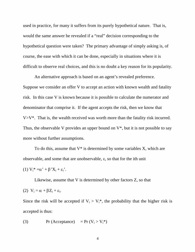
wealth to avoid potentially fatal risks, or accept wealth to take such risks, we are
implicitly defining a trade-off between wealth and the probability of death,
whether we like it or not. The ratio of the wealth we are willing to accept in
exchange for a small change in the probability of a fatality is expressed in units of
“dollars per death,” or the dollar value of a fatality. It is for this reason that this
trade-off is often called the value of a “statistical” life. The word “statistical” is
intended to make it clear that this is, despite its colloquial familiarity, a technical
term.
1. What is the VSL?
To make matters concrete, suppose that an economic agent is willing to
accept the consequences of an action that involves an increase of at least ΔW in
wealth in return for an increase in the probability of a fatality of ΔP. Then V*=
ΔW/ ΔP is an acceptable trade-off to that agent, and it is the VSL for the tradeoff
described by this particular fatality risk. V* need not be a constant, of course, and
would certainly be expected to depend on the level of P at which it is evaluated, a
person’s wealth, and perhaps many other factors, including personal preferences.
How is V* to be measured? It is apparent that V* is not directly observable,
so an indirect method is required for measurement. One possibility is simply to
ask the agent. Though this procedure has its advocates, and certainly has been
3
used in practice, for many it suffers from its purely hypothetical nature. That is,
would the same answer be revealed if a “real” decision corresponding to the
hypothetical question were taken? The primary advantage of simply asking is, of
course, the ease with which it can be done, especially in situations where it is
difficult to observe real choices, and this is no doubt a key reason for its popularity.
An alternative approach is based on an agent’s revealed preference.
Suppose we consider an offer V to accept an action with known wealth and fatality
risk. In this case V is known because it is possible to calculate the numerator and
denominator that comprise it. If the agent accepts the risk, then we know that
V>V*. That is, the wealth received was worth more than the fatality risk incurred.
Thus, the observable V provides an upper bound on V*, but it is not possible to say
more without further assumptions.
To do this, assume that V* is determined by some variables X, which are
observable, and some that are unobservable, ε, so that for the ith unit
(1) Vi* =α’ + β’Xi + εi’.
Likewise, assume that V is determined by other factors Z, so that
(2) Vi = α + βZi + εi.
Since the risk will be accepted if Vi > Vi*, the probability that the higher risk is
accepted is thus:
(3) Pr (Acceptance) = Pr (Vi > Vi*)
4
= Pr (εi - εi’ < α - α’ + βZi - β’Xi).
It is apparent that the average value of V among those who accept the risk,
E(V|Accept) = E(V|V>V*), must be at least as great as E(V*), the unconditional
average value of a statistical life among both those who accept and those who do
not accept the risk. Since the left hand side of equation (2) is only observed for
those who accept the risk, estimation of the parameters of equation (2) may suffer
from selection bias.
To make further progress further assumptions are required. Assume, for
example, that εi and εi’ are joint normally distributed, so that (3) can be estimated
by the probit function:
(4) Pr (Adoption) = F[(α - α’ + βZi - β’Xi)/σ],
where σ = σε - ε’ is (var (ε - ε’))1/2 and F[•] is the cumulative unit normal
distribution. It is apparent that even with this functional form assumption, it is
only possible to obtain estimates of (α - α’)/ σ, β/σ, β’/σ. The separate parameters
in equations (1) and (2) cannot be identified from this probit function alone.
However, since Vi is observable, it is possible to estimate (2) by the usual
selection corrected regression methods (Heckman 1979). In particular,
(5) E(Vi|acceptance) = α + βZi + ρσελi,
where ρ is the correlation between ε and ε’, λi = λ(Xi, Zi) = f(μ’Wi)/F(μ’Wi), and
μ’ consists of the vector [α - α’, β, -β’]’ and Wi the vector [1, Xi, Zi]. This model
5
is exactly identified, so that it is possible, in principle, to determine the parameters
of equation (1) and thus to calculate the average value of the VSL in the population
or for groups that have different values of X.2
The implementation of this model places very considerable demands on the
data typically available. In reality, the vast majority of studies settle for providing
estimates of V among those people who accept risks. Since this is the best
information that is often available, it is inevitable that we must rely on these
estimates for public decisions. However, it is important to consider the limitations
of this approach, just as it is important to consider the strengths.
2. How are estimates of the VSL used?
a. Traffic safety decisions
Some of the earliest use of VSL estimates, and an area that remains of great
practical importance, is in the design of highways.3 Though simplified, a large
number of government highway departments throughout the world engage in an
analysis of two key questions virtually daily: (1) Within a given budget, what is
the best way to allocate resources so as to reduce traffic fatalities? (2) Is the
budget sufficient to lower fatalities to the point where the typical driver would not
be willing to pay more for traffic safety. 2 See Ashenfelter and Greenstone (2004) for the details. 3 de Blaeij, Arianne, Raymond J.G.M. Florax, Piet Rietveld, and Erik Verhoef (2000) provide a detailed survey of estimates of the VSL derived from traffic safety data and decisions.
6
The first question does not require a measure of the VSL, but it does make
use of the key ingredients that make up that analysis. Suppose, for example, there
are 3 places on three different city streets where safety improvement projects could
be undertaken. And suppose that in these projects the cost of saving a life is 3.0
million, 1.0 million, and .5 million dollars, respectively. Clearly, allocating funds
to the third project is wiser than allocating funds to the other projects, as you get
more for your “safety buck.” For half a million dollars you can save a life, while
with the first project you must spend 6 times as much to do so. In short,
minimizing fatalities within a given budget requires calculation of the cost per
fatality saved, which is much like the calculation of V in the discussion above.
However, suppose that the total budget for safety projects in this city is 1.5
million dollars. Clearly, this means that only the second and third projects will be
undertaken. But is this optimal? The answer to this question depends on the VSL.
If the VSL is more than 3 million dollars, then clearly the third project should be
undertaken also, because the typical person is willing to give up more than 3
million dollars to save a life. Thus, the VSL plays a key determinant in discussions
of how big the traffic safety budget should be.
There does not seem to be a careful report of actual values used by highway
departments for the VSL, but even a little brief study will reveal that this approach
to highway safety is astonishingly widely used. For example, the state of
7
California’s department of transportation, Caltrans, uses $3,104,738 as the VSL,
and reports that the US Department of Transportation used a VSL value of $3
million as of January 2004.4 Although estimates of the VSL in the literature range
quite widely, from say $1 million to $8 million, it is my impression that highway
departments often use estimates at the bottom end of this range and sometimes
below it. If the VSL is higher than the one being used by the appropriate agency,
of course, the implication is that too many fatal accidents are taking place and that
the level of highway safety is sub-optimal.
b. Benefit-cost analysis of environmental regulations
The Environmental Protection Agency routinely makes use of the VSL
concept in the evaluation of the costs of environmental health and safety risks.5
The basic idea is to estimate fatality risks associated with a particular
environmental hazard and compel abatement to the point where the cost of an
additional life saved is greater than the VSL. This is, of course, the same use of
the VSL as in the analysis of traffic safety, although it is couched in different terms
and often leads some observers (not economists!) to rather different conclusions
about the merits of the approach.
4 See http://www.dot.ca.gov/hq/tpp/offices/ote/Benefit_Cost/benefits/accidents/value_estimates.html. This web site also provides a tutorial on just how to use the VSL to calculate the value of a highway safety improvement. 5 See Blomquist (2004) for a thoughtful review and summary of the VSL concept that was prepared at the request of the Environmental Protection Agency.
8
Of course, any decision by a government agency regarding safety has
implications for the VSL implied by that agency’s actions. Viscusi (2000)
provides an example of a number of implied estimates of the VSL from various US
government agency decisions. An interesting feature of these estimates is that
many of them lie far above the range of $1 to 8 million found in the literature.
This implies, of course, that some environmental rules have been adopted that may
be more stringent that would be optimal.
c. Medical interventions and technology
The use of the VSL in medicine is much the same as in the areas discussed
above, though measures of the value of a life saved take on their own special
dimensions.6 In effect, the adoption of a medical procedure is justified if its cost is
low enough compared to the life years it saves.
It is not difficult to convert a VSL to the value of a life year saved (LY). If
the VSL is based on the life of someone who is 40 years old, and if mortality
absent the intervention is 80, then a life saved corresponds to roughly 40 life years.
In this example, if the VSL is $4 million, then a VLY is $100 thousand. If an
intervention saves a life year and costs less than $100 thousand, it would be
considered cost effective using this standard.
6 The literature and discussion of this topic is enormous, and ranges from handbooks for practitioners to discussions of ethical issues related to the use of VSL measurements.
9
The value of a life year takes on special significance in medicine because a
life may be saved, but the person whose life is saved may have far less than a
normal, or even acceptable, quality of life. This leads to attempts to estimate
‘quality adjusted life years” (QALY). Needless to say, providing universally
acceptable measures of the quality of life can generate considerable controversy.
An unusual feature of estimates of the value of QALY is the widely cited
importance of a rough cut-off of $50 thousand. This estimate comes from the
national discussion of, and agreement to provide federal funds for, kidney dialysis
treatments on a universal basis in 1972 with the End-Stage Renal Disease
Amendment to the Medicare program, which extended coverage to patients under
the age of 65.7 Kidney dialysis costs roughly $50 thousand per year and its
provision is essential to provide a year of additional life to a patient with kidney
failure. Since kidney dialysis is clearly a treatment that has been revealed
preferred, it provides a lower bound on the value of a life year. It also provides, by
extension, a lower bound on the VSL when it is properly adjusted. It is important
to note that this method for bounding the VSL is really an application of the
procedure set out formally above, though it is my impression that the medical
profession discovered this method “independently” because its use is so natural.
7 See Weinstein (2005) for a very readable discussion of this and related issues in the cost-effective practice of medicine.
10
3. Problems in the measurement of a VSL
There are both conceptual issues to confront in the interpretation of
estimates of a VSL as well as potentially difficult measurement issues.
a. Endogeneity of risks
Perhaps the most important issue concerning the design of a study of the
VSL relates to the role of the conceptual experiment that the investigator is
designing. Is there an exogenous event that will affect wealth and fatality risk to
which we can observe an agent’s response? If there is, then it is possible to
measure the effect of the event on (a) wealth, and (b) fatality risk. The ratio of
these two effects, given that the event was accepted then provides an estimate of V
just as defined above and thus it provides a bound on the VSL.
However, such events are very difficult to isolate in practice. Consider, for
example, a driver’s choice of a speed. The reciprocal of the driver’s speed is the
hours it takes to travel a mile. Higher speeds reduce travel time, which is a form of
travel cost, and reducing travel time is something that, other things the same,
drivers prefer. At the same time, higher speeds will, given the condition and
congestion of a road, lead to a higher risk of fatality. This suggests that we might
consider the relation of speed to fatalities across roads as a measure of the causal
effect of speed (or the time it saves by faster driving) on fatalities.
11
It is not hard to see that the relation, across roads, between speed and
fatalities is not a causal one. Instead, both fatalities and speeds are, in part,
determined by a third factor, typical road condition and congestion level. When a
road is safe, drivers will sensibly increase their speeds. Thus the observed relation
between speed and fatalities across roads reflects two offsetting forces: one is that
increased speed causes more fatalities, and the other is that higher speeds result
from lower fatality risks. Whether the net effect is a positive or negative relation
between speed and fatalities is unclear, but one thing is clear: absent some further
assumptions, the resulting relationship does not reveal anything about the risk
trade-off posed by higher speeds and thus does not provide a way to bound the
VSL.8
A common approach to measuring the VSL uses the relation between wages
and fatality risks on jobs. However, it is rarely possible to compare identical jobs
that face different fatality risks, and the result is similar to the endogeneity problem
described above with respect to highway safety risks. The net relation between
wages and fatality risks contains both the causal effect due to the higher wage
demanded for higher fatality risks and the result of the effect of other factors (skill,
working conditions, etc.) that effect pay and are correlated with fatality risks across
8 In fact, empirically the net relation between speed and fatalities is near zero. See Ashenfelter and Greenstone (2004).
12
job types. Whether the net effect results in a positive or negative relation between
pay and fatality risk is unclear.9
b. Whose life is it, anyway?
It would be surprising if VSL did not vary across people with different
preferences, across income levels, and even over the life cycle. A natural question
to ask, therefore, of any VSL estimate is, just whose preferences are being
measured? There is, of course, a further question. Just whose preferences do we
want to measure?
In general the latter question is no doubt easier to answer than the first.
When public decisions are being made we normally would like to base decisions
on (and in a democratic society will base them on) the preferences of the central
agent, that is, neither the agent who loves risk the most nor the agent who hates
risk the most, but someone in the center of the distribution of preferences.
However, many useful studies of the VSL are naturally based on risk acceptance
behavior that is not in the center of the distribution, and in other cases it is unclear
whose preferences are being elicited.
For example, inexpensive, effective safety devices will be adopted by
virtually everyone, while expensive, ineffective safety devices will be adopted by
9 See especially Black and Kniesner (2003). In more than half of their specifications, they find that for male (and female) workers fatality risks are estimated as negatively related to wage rates, implying VSL estimates that are also negative. Also see Hersch (1998) who finds a negative association between injury rates and wages for all male workers. Many other studies find a positive relation between wage rates and fatality risks, including the earliest such estimate by Thaler and Rosen (1976).
13
few. As a result, the decision to adopt either of these two extreme types of devices
provides very weak bounds on the VSL of, say, the median agent.
An extreme example of this issue can arise in studies of the labor market.
Suppose that there are two jobs, one riskier than the other, and that the former
comprises the proportion θ of all jobs. Suppose also that there are two types of
workers, one that demands a higher premium for risky jobs than the other, and the
former comprises λ of the workers. Clearly, workers will be sorted into jobs so as
to minimize employer wage costs. If λ< θ, then the risky jobs can be filled with
workers who demand the low premium, while the reverse is the case if λ> θ. Thus,
the observed premium for risk depends critically on the sorting of workers and the
distribution of preferences as well as of risks. In the first case, if λ < .5 the
observed premium for risk will be less than the premium that would be demanded
if all workers were confronted with a risk. The reverse may, of course, also be the
case.
In principle, this discussion suggests that VSL’s measured from political
decisions that represent the center of the distribution of preferences are the most
appropriate for use in public policy decision making. However, these decisions
may suffer from other problems either because they do not, in fact, represent the
median preference or because the agents whose opinions are revealed are poorly
informed.
14
c. Do they know the risks?
A further problem is associated with the ability of agents to make informed
decisions in situations where safety risks are difficult for even experts to quantify.
In road safety most people have some appreciation or feeling for the risks
involved, though it is far from clear that extreme risks are well understood.
However, in medicine virtually everyone relies on the services of an expert or
doctor to assist in assessing risks. Likewise, many environmental risks are difficult
for even an expert to quantify.
In principle, the preferences revealed in the measurement of a VSL are not
based on misperceptions, but are accurate. However, even if they are not, it can be
argued that the trade-off between wealth and incorrect assessments of risk do
reveal the VSL so long as it is know what assessments the agents relied upon in
their decisions. Of course, eliciting the latter may be very difficult.10
d. Agency problems
It is often the goal to use a measure of a VSL in a public policy setting
where it is useful to avoid taking the issue for decision to the public directly
because doing so is excessively costly relative to the value of the decision.
Decisions such as the assignment of road repair priorities are obviously more
sensibly left to the highway department, for example, than to a public vote. Since
10 A review of the literature on this issue is contained in Blomquist (2004)
15
the VSL will be externally provided in the making of these decisions, it is apparent
that high standards are required for its measurement.
Thus, measures of the VSL based on what may only appear to be the
public’s preferences must be distinguished from measures that really are based on
those preferences. An especially difficult problem arises when the benefits from a
risk reduction are paid for by a group different from those whose risks are reduced.
Depending on the political power of the two groups, the observed decision may
differ considerably from a reasonable estimate of the VSL. Viscusi (2000)
provides many examples that might be interpreted from this perspective in the area
of environmental regulation. The evidence suggests that in these cases the benefits
of environmental regulations have been given greater weight than would be
consistent with most VSL measures. This suggests that environmental groups may
have played an important role in the regulatory process independent of what would
be implied by the concern for fatality risks, though this is a controversial issue and
there are other explanations for these findings.
4. An example of VSL measurement: speed limits
Although there have been a number of creative attempts designed to estimate
the value of a statistical life, there have been few opportunities to obtain estimates
based on the public’s willingness to accept an exogenous and known safety risk.
16
An analysis that does fall into this category is a study of highway safety risk
decisions that resulted from the opportunity that the federal government gave the
states in 1987 to choose a speed limit for rural interstate highways that was higher
than the uniform national maximum speed limit then in existence.11 This
remarkable natural experiment led 40 of the 47 states that have rural interstate
highways to adopt 65 mile per hour (mph) speed limits on them, while the
remaining 7 states retained 55 mph speed limits. The basic idea is to measure the
value of the time saved per incremental fatality created by the voluntary adoption
of an increased speed limit. Since adopters must have valued the time saved by
greater speeds more than the fatalities created, this ratio provides a convincing and
credible upper bound on the value of a statistical life (VSL).
Though far from perfect, this institutional change does make it possible to
address several conceptual problems noted above that have plagued attempts to
estimate the value of a statistical life. First, the 1987 law provides a credible
exogenous change in the safety environment. As a result it is possible to measure
the effects of this exogenous change on speeds and fatality rates. The ratio of these
two effects provides an estimate of V, the trade-off the parties faced in making
their decision. Second, many questions have been raised about the usefulness of
studies of the value of a statistical life when the decision makers studied may be
11 This example is based on Ashenfelter and Greenstone (2004).
17
poorly informed about the relevant risks. In this case the relevant decision makers
(i.e., state governments) were cognizant of the trade-offs associated with a change
in speed limits. Although this does not provide conclusive evidence that the
participants in the decisions were well informed, it is certainly more plausible than
is often the case. Third, any VSL estimate that is based on the decisions of a third
party (e.g., government policies) may not reflect the preferences of the group
whose VSL is of interest. Speed limit regulations, however, provide benefits
(reduced travel time) and costs (fatality risk) to precisely the same people, so that
appeals to a simple model of the typical voter are far more plausible in this context.
Finally, it seems perfectly reasonable to think that the voter whose preferences the
state governments represented are those of someone whose preferences are toward
the center of the distribution of preferences toward risk.
a. The history of speed limits in the US
The first laws imposing restrictive speed limits on motor vehicles were
passed in 1901 in Connecticut. It is not surprising that speed limits have been
enacted in places like Connecticut where congestion results in external effects on
other drivers from any driver’s speed. Indeed, the purpose of speed limits is to
reduce the variability in speeds that results in unacceptable fatality risks.12 Except
12 Indeed, an Indiana Department of Transportation reports states this explicitly: “Speed limits represent trade-offs between risk and travel time for a road class or specific highway section reflecting an appropriate balance between the societal goals of safety and mobility. The process of setting speed limits is not merely a technical exercise. It
18
for a brief period during the Second World War, the setting of speed limits
remained the responsibility of the state and local governments until 1974. In that
year Congress enacted the Emergency Highway Energy Conservation Act in
response to the perceived “energy crisis.” This bill, intended as a fuel conservation
measure, required, among other things, a national maximum speed limit of 55 mph.
This new national speed limit was lower than the existing maximum daytime speed
limit in all 50 states.
By 1976 the Federal Highway Administration began to enforce compliance
with the national speed limit. Each state was required to measure compliance with
the federal limit. States that did not enforce 50% compliance with the limit were
penalized by a 10 % reduction in federal highway funding. By 1987 dissatisfaction
with the federally imposed (and enforced) national maximum speed limit led
Congress to modify the law to permit states to set speed limits of 65 mph on rural
interstate highways only.
Even with the end of the concern for fuel conservation, the national
maximum speed limit was retained in some form until repeal in 1995.13 Despite
opposition, especially in the wide open Western states, much of the support for
involves value judgments and trade-offs that are in the arena of the political process” See Khan, Sinha, and McCarthy, 2000, p. 144.
13 By the end of 1997 only three states maintained a 55 mph speed limit on rural interstates: 20 states had
rural interstate speed limits of 65 mph, 16 were at 70 mph, 10 at 75 mph, and Montana had no daytime speed limit, returning to its policy in 1973.
19
national speed limits may have resulted from the unintended impact that this law
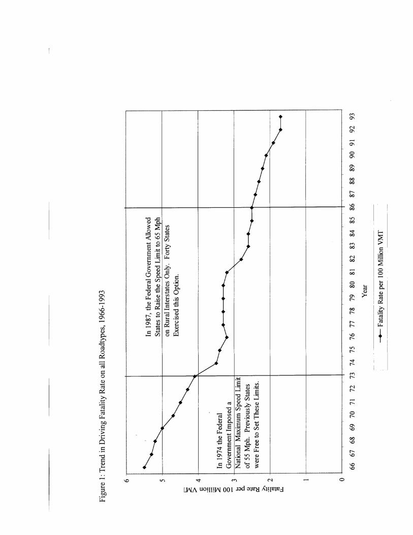
appeared to have on motor vehicle fatalities. Figure 1 shows the history of
fatalities per 100 million vehicle mile of travel (VMT) from 1966-93. It is
apparent that fatalities per mile traveled had been declining during this entire
period, but the decline of 15 percent (nearly 10,000 fatalities) immediately
following passage of the 1974 Emergency Highway Energy Conservation Act is
the largest ever recorded in a single year and was widely remarked upon at the
time.
b. Did speeds and fatality rates change?
Some very simple analyses of the impact of adopting the 65 mph speed limit
on rural interstates are reported in the top panel of Table 1. The basic idea is to
assume that, absent the adoption of the new speed limit, the change in speeds for
non-adopters on rural interstates would equal what it would have been for the
adopters had they not adopted the new speed limit. Thus the difference in these
differences provides a simple estimate of a “treatment” effect due to the speed
limit. It is important to determine whether actual speeds increased as, absent such
an increase there, is no actual natural experiment taking place. Thus, it is
important to measure the effect of the treatment on both actual speeds and on
fatalities.
20
Column (1) reports the raw unadjusted difference in differences (DD)
estimator of the effect of the 65 mph speed limit on fatality rates and speeds. This
is calculated as the difference between the mean fatality rates and speeds between
adopters and non-adopters from 1988-93 (i.e., the “post-period”) minus the same
difference from 1982-86 (i.e., the “pre-period”). This estimator suggests that the
adoption of the 65 mph speed limit increased fatality rates by 0.185 and speeds by
2.8 mph on rural interstates.14
The same analysis applied to the data on urban interstate and rural arterial
roads is contained in the bottom two panels of Table 1. These roadtypes were not
directly affected by the law change. They thus provide a test of whether they
might usefully serve as an additonal control group. The entries in the table indicate
that fatality rates decreased more in adopting states than non-adopting states on
both categories of roads.15 When these declines are viewed in the context of the
1982-86 levels, they appear modest. If these relative declines in adopting states are
due to an unobserved factor common to all roads in these states, then these roads
should be used as intra-state comparisons. It is evident that controlling for this
decline will increase the magnitude of the estimated effect of the 65 mph limit on
fatalities. Average speeds increased at about the same rate in adopting and non-
adopting states on these roadtypes. Interestingly, the speed data contradict the
21
popular “spillover” hypothesis that higher speed limits on one road cause drivers to
increase their driving speed on all roads.
Column (2) reports the results of the application of the DD estimator applied
to the ln transformation of the raw, state by roadtype by year data. The ln
difference approach is attractive because it provides estimates of (approximately)
proportionate changes in speeds and fatality rates. The estimates of the increased
speed limit imply proportionate increases of 0.31 in the fatality rate and of 0.045 in
speed. The estimated changes on urban interstates are quite small, at –0.063 and –
0.009, while they are even smaller at 0.005 and 0.008 on rural arterials. These
results suggest that it is worth considering the results of using both urban interstate
and rural arterial roads as additional control group for the analysis of rural
interstate road.
c. Estimates of the VSL
Estimates of an upper bound on the VSL are contained in Tables 2 and 3.
There two separate analyses because, in this case, the results depend on the precise
specification of the way the trade-off between travel time saved and fatality risks is
measured. In Table 2 the analysis is done using logarithmic (proportionate)
changes, while in the Table 3 the analysis is done in natural units. In each table
there are 10 different estimates of the VSL depending on which groups are used for
22
the comparison, adopters vs. non-adopters on rural interstates being used as a part
of the comparison throughout. The other estimates differ to the extent that urban
interstate and rural arterial roads are used as part of the control group for
comparison. They also differ in the extent to which detailed controls are used to
adjust for state, year, and roadtype changes that might confound estimates of the
effect of the speed limit on speeds and fatalities.
For each specification in each table there are three numbers. The first is the
estimate of the trade-off between hours saved and fatality risk.16 The second is the
estimate of the standard error of the parameter estimated, while the third is
transformed by the value of time to provide a measure of the VSL.
It is apparent from the tables that the estimates of the VSL are fairly
sensitive to the specification assumed for the analysis, though the range of
estimates may provide a workable basis for broad conclusions. Using the rural
interstate roads as comparators only, the estimates of the VSL are $1.6 million for
the analysis in levels and $6.0 million for the analysis in logarithms. In general,
this difference is typical of those in the tables and these two numbers provide
pretty representative estimates from each table, though smaller and larger VSL
estimates can be found in them. The primary advantage of these estimates is the
extent to which they can withstand scrutiny based on the conceptual issues
16 These are estimates of a regression of the hours it takes to travel a mile on fatalities, with the state-year interaction associated with the adoption of the 65 mile per hour speed limit used as an instrumental variable for fatalities.
23
associated with measuring the VSL. Their biggest disadvantage is that they are not
unambiguously independent of the specification used to produce them.
4. Prospects
It has been just thirty years during which economists have defined,
quantified, and critiqued the operational definition of safety risks summarized as
the Value of a Statistical Life. Looking back, this is quite a remarkable
accomplishment. The basic theory is both widely understood and taught, but also
used in public decisions in many areas. Measurements of the VSL are essential for
decisions based on these ideas, and apparently the precision of the estimates we
have is considered better than the use of no measurements at all. Of course, there
is room for much improvement, and no doubt there will be a great deal of it.
24
25

26
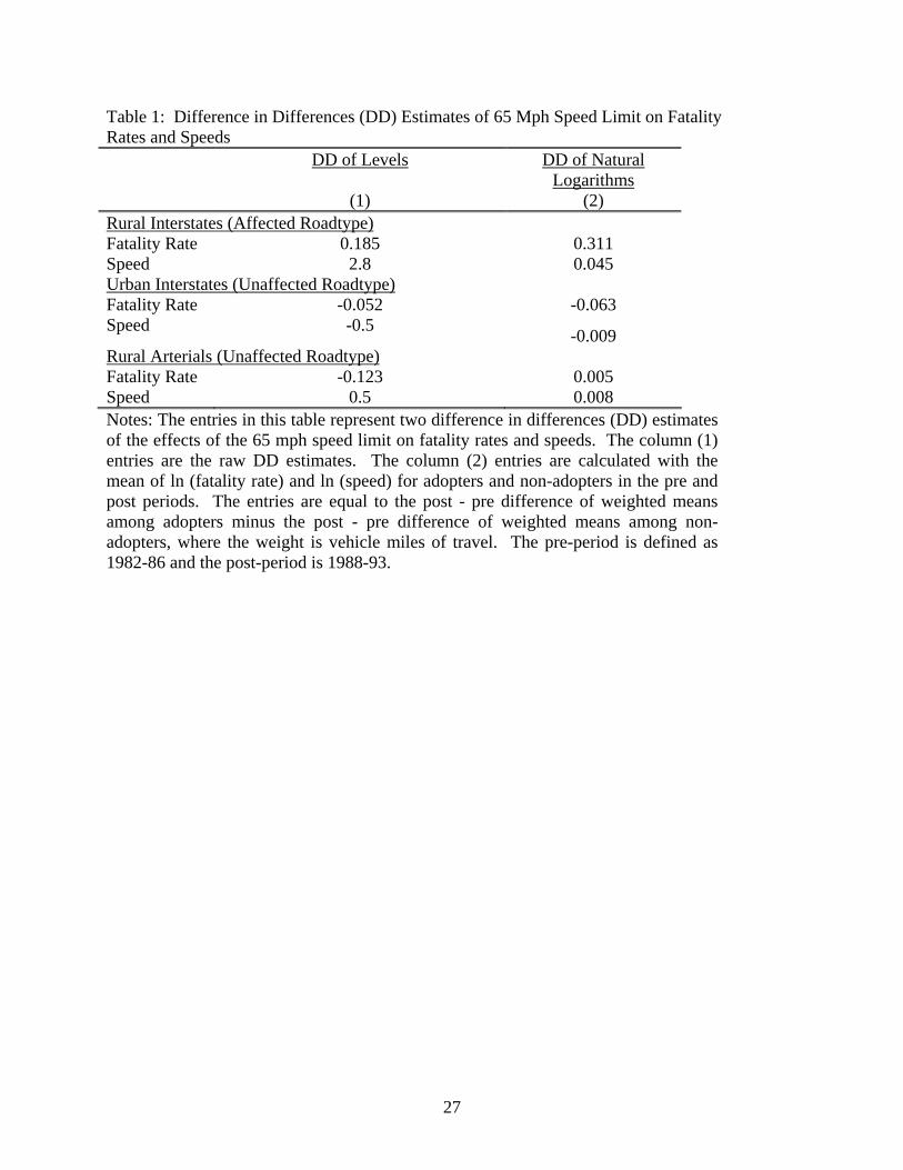
Table 1: Difference in Differences (DD) Estimates of 65 Mph Speed Limit on Fatality Rates and Speeds DD of Levels DD of Natural
Logarithms (1) (2) Rural Interstates (Affected Roadtype) Fatality Rate 0.185 0.311 Speed 2.8 0.045 Urban Interstates (Unaffected Roadtype) Fatality Rate -0.052 -0.063 Speed -0.5 -0.009 Rural Arterials (Unaffected Roadtype) Fatality Rate -0.123 0.005 Speed 0.5 0.008 Notes: The entries in this table represent two difference in differences (DD) estimates of the effects of the 65 mph speed limit on fatality rates and speeds. The column (1) entries are the raw DD estimates. The column (2) entries are calculated with the mean of ln (fatality rate) and ln (speed) for adopters and non-adopters in the pre and post periods. The entries are equal to the post - pre difference of weighted means among adopters minus the post - pre difference of weighted means among non-adopters, where the weight is vehicle miles of travel. The pre-period is defined as 1982-86 and the post-period is 1988-93.
27
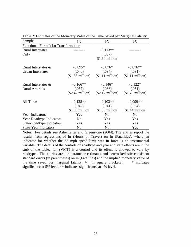
Table 2: Estimates of the Monetary Value of the Time Saved per Marginal Fatality Sample (1) (2) (3) Functional Form I: Ln Transformation Rural Interstates --------- -0.113** --------- Only (.037) [$1.64 million] Rural Interstates & -0.095* -0.076* -0.076** Urban Interstates (.040) (.034) (.031) [$1.38 million] [$1.11 million] [$1.11 million] Rural Interstates & -0.166** -0.146* -0.122* Rural Arterials (.057) (.066) (.051) [$2.42 million] [$2.12 million] [$1.78 million] All Three -0.128** -0.103** -0.099** (.042) (.041) (.034) [$1.86 million] [$1.50 million] [$1.44 million] Year Indicators Yes No No Year-Roadtype Indicators No Yes Yes State-Roadtype Indicators Yes Yes Yes State-Year Indicators No No Yes Notes. For details see Ashenfelter and Greenstone (2004). The entries report the results from regressions of ln (Hours of Travel) on ln (Fatalities), where an indicator for whether the 65 mph speed limit was in force is an instrumental variable. The details of the controls on roadtype and year and state effects are in the stub of the table. Ln (VMT) is a control and its effect is allowed to vary by roadtype. The entries are the parameter estimates and heteroskedastic consistent standard errors (in parentheses) on ln (Fatalities) and the implied monetary value of the time saved per marginal fatality, V, [in square brackets]. * indicates significance at 5% level, ** indicates significance at 1% level.
28

Table 3: Estimates of the Monetary Value of the Time Saved per Marginal Fatality Sample (1) (2) (3) Functional Form II: Untransformed Rural Interstates --------- 17.03* --------- Only (7.67) [$5.92 million] Rural Interstates & 25.64** 16.39* 8.65* Urban Interstates (9.42) (7.46) (3.84) [$8.91 million] [$5.69 million] [$3.00 million] Rural Interstates & 4.01** 8.25 7.88* Rural Arterials (0.51) (4.32) (3.79) [$1.39 million] [$2.87 million] [$2.74 million] All Three 6.97** 11.98* 8.80** (1.16) (5.06) (3.57) [$2.42 million] [$4.16 million] [$3.06 million] Year Indicators Yes No No Year-Roadtype Indicators No Yes Yes State-Roadtype Indicators Yes Yes Yes State-Year Indicators No No Yes Notes: The entries report the results from regressions of speed on fatality rates, where an indicator for whether the 65 mph speed limit was in force is an instrumental variable. The equation is weighted by the square root of VMT. The details of the controls on roadtype and year and state effects are in the stub of the table. The entries are the parameter estimates and heteroskedastic consistent standard errors (in parentheses) on the fatality rate and the implied monetary value of the time saved per marginal fatality, V, [in square brackets]. * indicates significance at 5% level, ** indicates significance at 1% level
29
References Ashenfelter, Orley and Michael Greenstone. “Using Mandated Speed Limits to Measure the Value of a Statistical Life,” Journal of Political Economy, 112 (2004): S226- S267. Black, Dan A. and Thomas J. Kniesner. “On the Measurement of Job Risk in Hedonic
Wage Models.” Mimeograph, University of Syracuse, March 2003. Blomquist, Glenn C. “Self Protection and Averting Behavior, Values of Statistical Lives, and Benefit Cost Analysis of Environmental Policy.” Review of Economics of the Household 2 (2994): 89-110. de Blaeij, Arianne, Raymond J.G.M. Florax, Piet Rietveld, and Erik Verhoef. “The
Value of a Statistical Life in Road Safety: A Meta-Analysis.” Tinbergen Institute Discussion Paper No. 2000-089/3, 2000.
Heckman, James J. “Sample Selection Bias as a Specification Error.” Econometrica, 47 (1979): 153-62. Hersch, Joni. “Compensating Differentials for Gender-Specific Injury Risks.”
American Economic Review 88(1998): 598-607. Khan, Nisar, Kumares C. Sinha, and Patrick S. McCarthy. “An Analysis of Speed Limit
Policies for Indiana.” FHWA/IN/JTRP-99/14, Joint Transportation Research Project, Purdue University, West Lafayette, IN, 2000. American Economic Review 88(1998): 598-607.
Thaler, Richard, and Rosen, Sherwin. “The Value of Saving a Life: Evidence from the Labor Market,” in Household Production and Consumption. Nestor E. Terleckyj, ed., Cambridge, MA: NBER, 1976: 265 – 298.
Viscusi, W. Kip. “The Value of Life in Legal Contexts: Survey and Critique.” American Law and Economics Review, 2 (2000): 195-222. Weinstein, Milton. “Spending Health Care Dollars Wisely: Can Cost-Effectiveness Analysis Help?” Policy Brief No. 30/2005, Syracuse University, 2005.
30