HAL Id: hal-00634765https://hal.archives-ouvertes.fr/hal-00634765

Submitted on 23 Oct 2011

HAL is a multi-disciplinary open accessarchive for the deposit and dissemination of sci-entific research documents, whether they are pub-lished or not. The documents may come fromteaching and research institutions in France orabroad, or from public or private research centers.

L’archive ouverte pluridisciplinaire HAL, estdestinée au dépôt et à la diffusion de documentsscientifiques de niveau recherche, publiés ou non,émanant des établissements d’enseignement et derecherche français ou étrangers, des laboratoirespublics ou privés.

Measuring Transient Temperature of the Medium inPower Engineering Machines and Installations

Magdalena Jaremkiewicz, Dawid Taler, Tomasz Sobota

To cite this version:Magdalena Jaremkiewicz, Dawid Taler, Tomasz Sobota. Measuring Transient Temperature of theMedium in Power Engineering Machines and Installations. Applied Thermal Engineering, Elsevier,2010, 29 (16), pp.3374. �10.1016/j.applthermaleng.2009.05.013�. �hal-00634765�

Accepted Manuscript

Measuring Transient Temperature of the Medium in Power Engineering Ma‐

chines and Installations

Magdalena Jaremkiewicz, Dawid Taler, Tomasz Sobota

PII: S1359-4311(09)00164-1

DOI: 10.1016/j.applthermaleng.2009.05.013

Reference: ATE 2815

To appear in: Applied Thermal Engineering

Received Date: 23 September 2008

Revised Date: 8 May 2009

Accepted Date: 16 May 2009

Please cite this article as: M. Jaremkiewicz, D. Taler, T. Sobota, Measuring Transient Temperature of the Medium

in Power Engineering Machines and Installations, Applied Thermal Engineering (2009), doi: 10.1016/

j.applthermaleng.2009.05.013

This is a PDF file of an unedited manuscript that has been accepted for publication. As a service to our customers

we are providing this early version of the manuscript. The manuscript will undergo copyediting, typesetting, and

review of the resulting proof before it is published in its final form. Please note that during the production process

errors may be discovered which could affect the content, and all legal disclaimers that apply to the journal pertain.

ACCEPTED MANUSCRIPT

Measuring Transient Temperature of the Medium in Power Engineering Machines

and Installations

Magdalena Jaremkiewicz*, Dawid Taler**, Tomasz Sobota***

*) ***) Cracow University of Technology, Division of Power Engineering,

al. Jana Pawła II 37, PL-31-864 Kraków, Poland

**) University of Science and Technology, Department of Power Installations

al. Mickiewicza 30, PL-30-059 Kraków, Poland

***) corresponding author, e-mail: tsobota@mech.pk.edu.pl

Abstract: Under steady-state conditions when fluid temperature is constant, there is no damping

and time lag and temperature measurement can be made with high accuracy. But when fluid

temperature is varying rapidly as during start-up, quite appreciable differences occur between

the true temperature and the measured temperature because of the time required for the transfer

of heat to the thermocouple placed inside a heavy thermometer pocket. In this paper, two

different techniques for determining transient fluid temperature based on the first and second

order thermometer model are presented. The fluid temperature was determined using measured

thermometer temperature, which is suddenly immersed into boiling water. To demonstrate the

applicability of the presented method to actual data, the air temperature which changes in time,

was calculated based on the temperature readings from the sheathed thermocouple.

1. Introduction

Most books on temperature measurement concentrate on steady-state measurements of

fluid temperature [1-9]. Only a unit-step response of thermometers is considered to

estimate the dynamic error of temperature measurement.

ACCEPTED MANUSCRIPT

Little attention is paid to measurements of transient fluid temperature, despite the great

practical significance of the problem [10-14]. In [7] a thermocouple compensating

network is applied to increase the frequency response of the thermocouple. The

disadvantage of the compensating network is that it educes the thermocouple output and

is appropriate for the time independent time constant. When a temperature measurement

is conducted under unsteady conditions, it is of great importance that the dynamic

measurement errors should be taken into account [12, 13]. If the dynamic response of

the thermometers had been modelled then the better agreement between the

experimental data and model predictions would have been achieved.

The measurement of the transient temperature of steam or flue gases in thermal power

stations is very difficult. Massive housings and low heat transfer coefficient cause the

actually measured temperature to differ significantly from the actual temperature of the

fluid.

Some particularly heavy thermometers may have time constants of 3 minutes or more,

thus requiring about 15 minutes to settle for a single measurement.

There are some thermometer designs where there is more than one time constant

involved. In order to describe the transient response of a temperature sensor immersed

in a thermowell, the measuring of the medium in a controlled process may have two or

three time constants which characterise the transient thermometer response.

The problem of a dynamic error during the measuring of the temperature of the

superheated steam is particularly important for the superheated steam temperature

control systems which use injection coolers. Due to a large inertia of the thermometer, a

correct measurement of the transient temperature of the fluid, and thus the automatic

control of the superheated steam temperature is far from perfect. A similar problem is

ACCEPTED MANUSCRIPT

encountered in flue gas temperature measurements, since the thermometer time constant

and time delay are large.

In this paper two methods of determining the changing in time temperature of the

flowing fluid on the basis of the temperature time changes indicated by the thermometer

are presented.

In the first method the thermometer is considered to be a first order inertia device and in

the second method it is considered to be a second order inertia device. A local

polynomial approximation, based on 9 points was used for the approximation of the

temperature changes. This assures that the first and the second derivative from the

function representing the thermometer temperature changes in time will be determined

accurately.

An experimental analysis of the industrial thermometer at the step increase of the fluid

temperature was conducted. A comparison was made between the temperature time

histories determined using the two proposed methods at the step increase of the fluid

temperature were compared.

2. Mathematical models of the thermometers

Usually the thermometer is modelled as an element of the concentrated thermal

capacity. In this way, it is assumed that the temperature of the thermometer is only the

function of time and temperature differences occurring within the thermometer are

neglected. The temperature changes of the thermometer in time T(t) have been

described by an ordinary first order differential equation (first order thermometer

model)

cz

dTT T

dt . (1)

ACCEPTED MANUSCRIPT

For thermometers with a complex structure used for measuring the temperature of the

fluid under high pressure, the accuracy of the first order model (1) is inadequate.

3. Thermometer of a complex structure

To demonstrate that a dynamic response of a temperature sensor placed in a housing

may be descried by a second-order differential equation, a simple thermometer model

shown in Fig. 1 will be considered.

An air gap can appear between the external housing and the temperature sensor. The

thermal capacity of this air gap cρ is neglected due to its small value (Fig. 1).

Introducing the overall heat transfer coefficient kw referenced to the internal surface of

the housing and accounting for the radiation heat transfer from the housing to the inner

sensor, we obtain:

11 1 1

4w w w

w w p T

D d D d D

k d

. (2)

The heat balance equation for the sensor located within the housing assumes the form:

4 4w w o o

dTA c P k T T C T T

dt , (3)

where

1 11

T w o

dC

dD

.

Introducing the overall heat transfer coefficient kz for the housing referenced to its

external surface, we obtain:

11 1

2z w o

z z o

D D

k

. (4)

ACCEPTED MANUSCRIPT

The formulas (2) and (4) for the overall heat transfer coefficients were derived using the

basic principles of heat transfer [2, 4, 8]. The heat transfer equation for the housing

(thermowell) can be written in the following form:

4 4oo o o z z cz o w w o o

dTA c P k T T P k T T C T T

dt . (5)

In the analysis of the heat exchange between the housing and the thermocouple the

radiation heat transfer will also be disregarded. Such a situation occurs, when a gap

between the housing and temperature sensor is filled with non-transparent substance or

one of the two emissivities εo and εT is close to zero.

After determining the temperature To from Eq.(3), we obtain:

ow w

A c dTT T

P k dt

. (6)

Substituting Eq. (6) into Eq. (5) yields

2

21o o o z zo o o

czw w z z z z w w o o o o o o

A c A c P k A cA cd T A c dTT T

P k P k dt P k P k A c A c dt

. (7)

Let us next to define the following coefficients in Eq. (7)

2 ,o o o

w w z z

A c A ca

P k P k

1 1 ,z zo o o

z z w w o o o o o o

P k A cA c A ca

P k P k A c A c

a0 = 1, b0 = 1,

to obtain the ordinary differential equation of the second order

2

2 12 cz

d T dTa a T T

dt dt . (8)

The initial conditions assume the form of:

00 0T T ,

0

0T

t

dT tv

dt

. (9)

ACCEPTED MANUSCRIPT

The initial problem (8-9) was solved using the Laplace transformation. The operator

transmittance G(s) assumes the following form:

1 2

1

( ) 1 1cz

T sG s

T s s s

. (10)

The time constants 1 and 2 are determined using the formula:

21,2 2

1 1 2

2

4

a

a a a

. (11)

The differential Equation (8) can be written in the following form:

2

1 2 1 22 cz

d T dTT T

dt dt . (12)

For the step increase of the fluid temperature from 0 to the constant value Tcz the

Laplace transform of the fluid temperature assumes the form: czcz

TT s

s and the

transmittance formula can be simplified to:

1 2

1

1 1cz

T s

T s s s

. (13)

After writing Eq. (12) in the form:

1 2

2 1 2 1

1 2

1 1 1

1 1cz

T s

T ss s

(14)

it is easy to find the inverse Laplace transformation and determine the thermometer

temperature as a function of time:

1 2

2 1 1 2 1 2

1 exp expcz

T t t tu t

T

. (15)

For the first order model the thermometer response for a unit step fluid temperature

change is determined by the simple expression:

ACCEPTED MANUSCRIPT

1 expt

u t

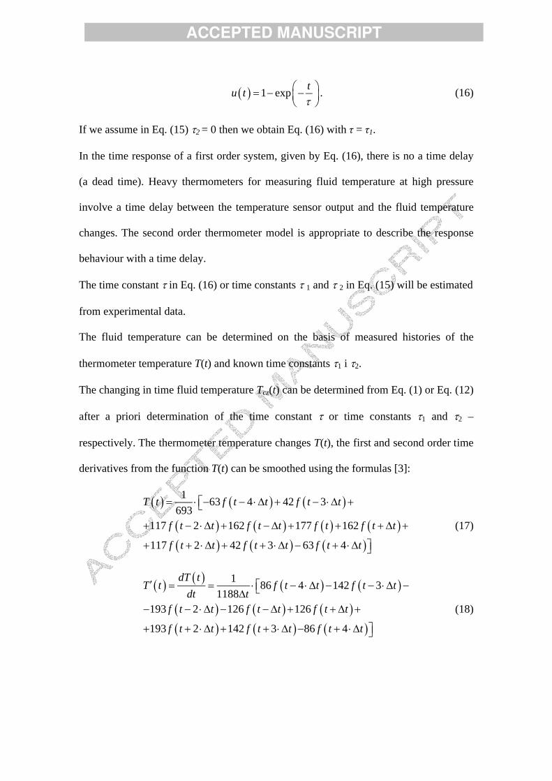
. (16)

If we assume in Eq. (15) 2 = 0 then we obtain Eq. (16) with τ = τ1.

In the time response of a first order system, given by Eq. (16), there is no a time delay

(a dead time). Heavy thermometers for measuring fluid temperature at high pressure

involve a time delay between the temperature sensor output and the fluid temperature

changes. The second order thermometer model is appropriate to describe the response

behaviour with a time delay.

The time constant in Eq. (16) or time constants 1 and 2 in Eq. (15) will be estimated

from experimental data.

The fluid temperature can be determined on the basis of measured histories of the

thermometer temperature T(t) and known time constants 1 i 2.

The changing in time fluid temperature Tcz(t) can be determined from Eq. (1) or Eq. (12)

after a priori determination of the time constant or time constants 1 and 2 –

respectively. The thermometer temperature changes T(t), the first and second order time

derivatives from the function T(t) can be smoothed using the formulas [3]:

163 4 42 3

693117 2 162 177 162

117 2 42 3 63 4

T t f t t f t t

f t t f t t f t f t t

f t t f t t f t t

(17)

186 4 142 3

1188193 2 126 126

193 2 142 3 86 4

dT tT t f t t f t t

dt tf t t f t t f t t

f t t f t t f t t

(18)

ACCEPTED MANUSCRIPT

2

22

128 4 7 3

462

8 2 17 20 17

8 2 7 3 28 4 ,

d T tT t f t t f t t

dt t

f t t f t t f t f t t

f t t f t t f t t

(19)

in order to eliminate, at least partially, the influence of random errors in the

thermometer temperature measurements T(t) on the determined fluid temperature Tcz(t).

The symbol f(t) in Eq. (17-19) denotes the temperature indicated by the thermometer

and t is a time step.

If measured temperature histories are not too noisy, the first and second order can be

approximated by the central difference formulas

2

f t t f t tT t

t

, (20)

2

2f t t f t f t tT t

t

. (21)

Equation (1) and Equation (2) can also be used for determining fluid temperature Tcz

when the time constants of the thermocouple τ or τ1 and τ2 are a function of fluid

velocity u.

After substituting the time constant τ(w) into Eq. (1) we can determine fluid temperature

Tcz(t) for different fluid velocities using the proposed method.

4. Experimental determination of time constants

The method of least squares was used to determine the time constants τ1 and τ2 in Eq.

(15) or the time constant τ in Eq. (16). The values for the time constants are found by

minimising the function S

ACCEPTED MANUSCRIPT

2

1

minN

m i ii

S u t u t

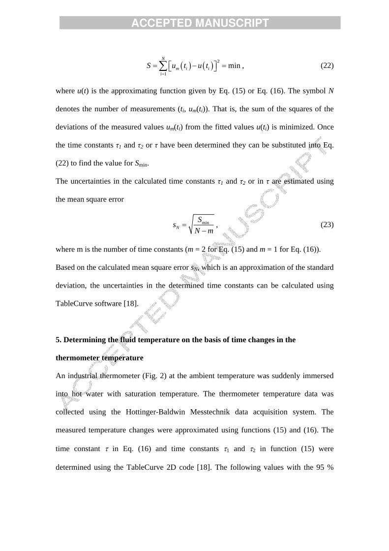
, (22)

where u(t) is the approximating function given by Eq. (15) or Eq. (16). The symbol N

denotes the number of measurements (ti, um(ti)). That is, the sum of the squares of the

deviations of the measured values um(ti) from the fitted values u(ti) is minimized. Once

the time constants τ1 and τ2 or τ have been determined they can be substituted into Eq.

(22) to find the value for Smin.

The uncertainties in the calculated time constants τ1 and τ2 or in τ are estimated using

the mean square error

minN

Ss

N m

, (23)

where m is the number of time constants (m = 2 for Eq. (15) and m = 1 for Eq. (16)).

Based on the calculated mean square error sN, which is an approximation of the standard

deviation, the uncertainties in the determined time constants can be calculated using

TableCurve software [18].

5. Determining the fluid temperature on the basis of time changes in the

thermometer temperature

An industrial thermometer (Fig. 2) at the ambient temperature was suddenly immersed

into hot water with saturation temperature. The thermometer temperature data was

collected using the Hottinger-Baldwin Messtechnik data acquisition system. The

measured temperature changes were approximated using functions (15) and (16). The

time constant in Eq. (16) and time constants 1 and 2 in function (15) were

determined using the TableCurve 2D code [18]. The following values with the 95 %

ACCEPTED MANUSCRIPT

confidence uncertainty were obtained: = 14.07 ± 0.39 s, 1 = 3.0 ± 0.165 s, and 2 =

10.90 ± 0.2 s.

Next, the fluid temperature changes were determined from Eq. (1) for the first order

model and from Eq. (12) for the second order model (Fig. 3). The time step t was

1.162 s.

The analysis of the results presented in Fig. 3 indicates that the second order model

delivers more accurate results.

The same tests were repeated for sheathed thermocouple with outer diameter 1.5 mm

and the results are presented in Fig. 4. The estimated value of the time constant and the

uncertainty at 95 % confidence are: τ = 1.54 ± 0.09 s. As the thermocouple is thin, then

Eq. (16) was used as the function approximating the transient response of the

thermocouple. First, the transient fluid temperature czT u t was calculated using Eq.

(1) together with Eqs. (17) i (18). Then, the raw temperature data was used. The first

order time derivative dT dt in Eq. (1) was calculated the central difference quotient

(20). The inspection of the results displayed in Fig. 4 indicates, that both approaches

give practically the same results.

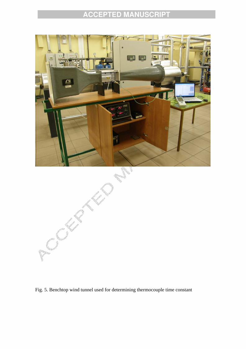
The thermocouple time constant τ for various air velocities w, were determined in the

open benchtop wind tunnel (Fig. 5). The WT4401-S benchtop wind tunnel is designed

to give a uniform flow rate over 100 mm × 100 mm test cross section [17].

The experimental data points displayed in Fig. 6 were approximated by the least squares

method. The following function was obtained:

1

a b w

, (24)

where τ is expressed in s, and w in m/s.

ACCEPTED MANUSCRIPT

The best estimates for the constants a and b, with the 95 % confidence uncertainty in the

results, are: a = 0.009526 ± 0.001405 1/s and b = 0.063436 ± 0.002338 1 2m s

.

The variations of the thermocouple time constant τ with the fluid velocity for the

sheathed thermocouple with the outer diameter of 1.5 mm are shown in Fig. 6.

The time constant of the thermocouple T T Tm c / A depends strongly on the heat

transfer coefficient αT on the outer thermometer surface, which in turn is a function of

the air velocity [19]. In order to demonstrate the applicability of the presented method to

actual data, the air temperature Tcz(t) in the wind tunnel will be determined based on the

measured air temperature with the sheathed K-thermocouple with an outer diameter of

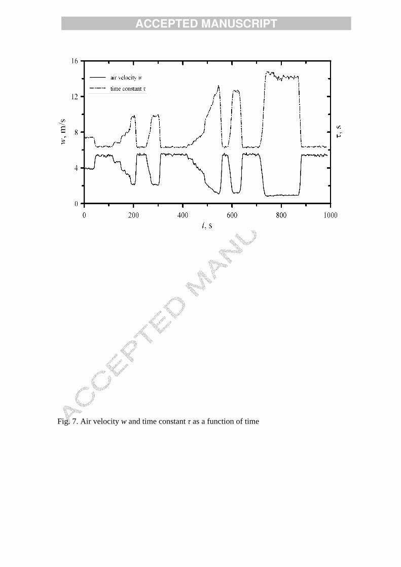
1.5 mm. The flowing air was heated by the plate fin and tube heat exchanger. The air

velocity w and thermocouple temperature are shown in Figs 7 and 8. The time constant τ

was calculated using Eq. (24). The air temperature Tcz(t) was determined from Eq. (1).

The time derivative dT/dt in Eq. (1) was calculated using Eq. (18) (9-point moving

averaging filter) or Eq. (20) (central difference quotient).

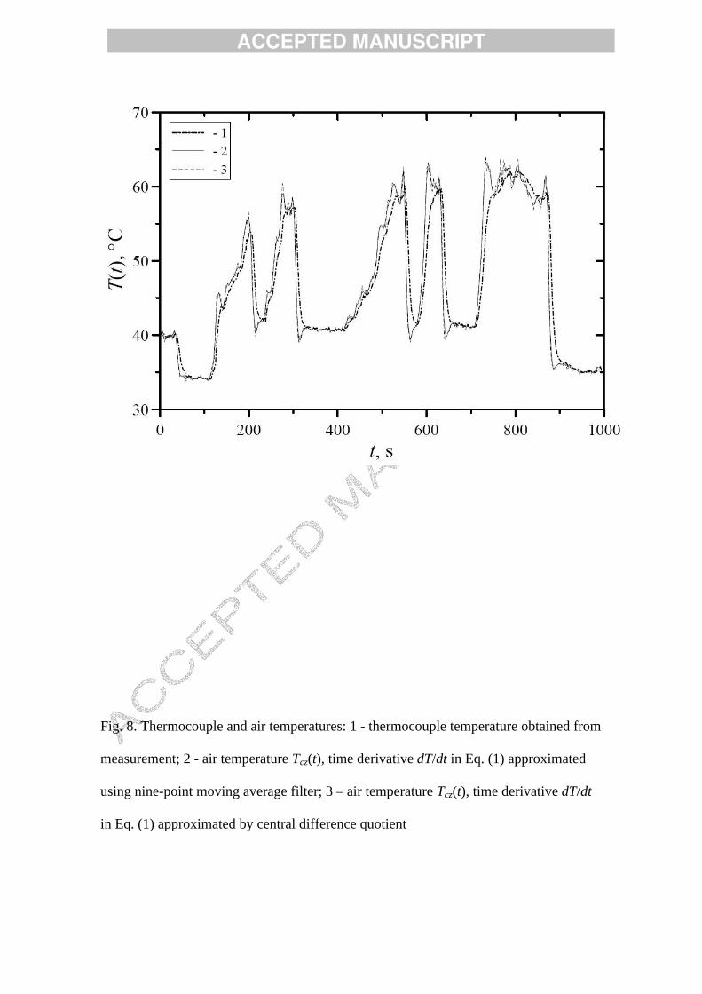
The coincidence of the obtained results is very good (Fig. 8).

The measured temperature T(t) was not too noisy, so, the time derivative dT/dt in Eq.

(1) might be calculated using the central difference approximation (20) to give the

smooth air temperature history (Fig. 8).

It can be seen that the calculated air temperature Tcz(t) differ significantly from the

temperature T(t) indicated by the thermocouple (Fig. 9) as the time constant τ(t) is large.

6. Conclusions

Both methods of measuring the transient temperature of the fluid presented in this paper

can be used for the on-line determining fluid temperature changes as a function of time.

ACCEPTED MANUSCRIPT

The first method in which the thermometer is modelled using the ordinary, first order

differential equation is appropriate for thermometers which have very small time

constants. In such cases the delay of the thermometer indication is small in reference to

the changes of the temperature of the fluid. For industrial thermometers, designed to

measure temperature of fluids under a high pressure there is a significant time delay of

the thermometer indication in reference to the actual changes of the fluid temperature.

For such thermometers the second order thermometer model, allowing for modelling the

signal delay, is more appropriate. Large stability and accuracy of the determination of

the actual fluid temperature on the basis of the time temperature changes indicated by

the thermometer can be achieved by using a 9 point digital filter.

Fluid temperature changes obtained using the two described methods were compared. It

was established that the thermometer model of the second order gave better results for

the industrial thermometer with the large thermowell. The techniques proposed in the

paper can also be used, when time constants are functions of fluid velocity.

Nomenclature

A – surface area of the thermocouple cross section, m2,

Ao – surface area of the housing cross section, m2,

AT – outer surface area of the thermocouple, m2,

c – average specific heat of the thermocouple, J/(kgK),

co – average specific heat of the housing, J/(kgK),

d – outer diameter of the thermocouple, m,

Dw – inner diameter of the housing, m,

ACCEPTED MANUSCRIPT

Dz – outer diameter of the housing, m,

kw – overall heat transfer coefficient between the housing inner surface and outer

surface of the thermocouple referenced to the inner housing surface, W/(m2K)

kz – overall heat transfer coefficient between the fluid and the housing referenced to

the outer housing surface, W/(m2K)

mT – thermocouple mass, kg

Pw – perimeter of the internal surface of the housing, m,

s – complex variable,

Tcz – fluid temperature, C,

To – housing temperature, C,

T0 – initial thermometer temperature, C,

czT s – Laplace transform of the fluid temperature,

T s – Laplace transform of the thermometer temperature

u – unit-step response of the thermometer,

w – air velocity, m/s

Greek symbols

T – heat transfer coefficient on the outer surface of the thermocouple, W/(m2K),

w – heat transfer coefficient on the inner surface of the housing, W/(m2K),

z – heat transfer coefficient on the outer surface of the housing, W/(m2K),

o – housing thickness, m,

εo – emissivity of the housing inner surface,

εT – emissivity of the thermocouple surface,

ACCEPTED MANUSCRIPT

– housing thermal conductivity, W/(mK),

p – thermal conductivity of the air gap, W/(mK),

– average density of the thermocouple, kg/m3,

– average density of the housing, kg/m3,

σ – Stefan-Boltzmann constant, 85.67 10 W/(m2K4),

– time constant of the thermometer in the first order model, s,

– time constants of the thermometer in the second order model, s

References

[1] J. V. Nicholas, D. R. White, Traceable Temperatures. An Introduction to

Temperature Measurement and Calibration, Second Edition, John Wiley & Sons,

New York, 2001, 140-145.

[2] L. Michalski, K. Eckersdorf and J. McGhee, Temperature Measurement, Wiley,

Chichester, 1991, 251-316.

[3] S. Wiśniewski, Temperature Measurement in Engines and Thermat Facilities,

WNT, Warszawa, 1983, 281-335 (in Polish).

[4] J. Taler, Theory and Practice of Identification of Heat Transfer Prosesses, Zakład

Narodowy imienia Ossolińskich, Wrocław, 1995, 38-90 (in Polish).

[5] Z. Kabza, K. Kostyrko, S. Zator, A. Łobzowski, W. Szkolnikowski, Room

Climate Control, Agenda Wydawnicza, Pomiary Automatyka Kontrola,

Warszawa, 2005, 58-75 (in Polish).

[6] M. W. Jervis, D. A. L. Clinch, J. M. Wignall, K. J. Bradburry, R. F. E. Crump, J.

Grant, J. W. Tootell, G. H. D. Keen, J. Jenkinson, N. Broadhead, Control and

ACCEPTED MANUSCRIPT

Instrumentation, in: Modern Power Station Practice, Pergamon Press, Oxford,

1991, 110-142.

[7] J. P. Holman, Experimental Methods for Engineers, McGraw-Hill, Boston, 2001,

399-404.

[8] O. A. Gerashchenko, A. N. Gordov, V. I. Lakh, B. I. Stadnyk, N. A. Yaryshev,

Temperature Measurement, Naukova dumka, Kiev, 1984, 66-73 (in Russian).

[9] J. C. Han, S. Dutta, S. V. Ekkad, Turbine Heat Transfer and Cooling Technology,

Taylor & Francis, New York, 2000, 531-584.

[10] V. Székely, S. Ress, A. Poppe, S. Török, D. Magyari, Zs. Benedek, K. Torki, B.

Courtois, M. Rencz, New approaches in the transient thermal measurements,

Microelectronics Journal 31 (2000) 727–733.

[11] D. S. Crocker, M. Parang, Unsteady temperature measurement in an enclosed

thermoconvectively heated air, Int. Comm. Heat Mass Transfer, Vol. 28, No. 8,

(2001) 1015-1024.

[12] A. Mawire, M. McPherson, Experimental and simulated temperature distribution

of oil-pebble bed thermal energy storage system with a variable heat source,

Applied Thermal Engineering 29 (2009) 1086-1095.

[13] Z. Li, M. Zheng, Development of a numerical model for the simulation of vertical

U-tube ground exchangers, Applied Thermal Engineering 29 (2009) 920-924.

[14] P. C. Chau, Process Control. A First Course with MATLAB, Cambridge

University Press, Cambridge, 2002, 44-63.

[15] ASME: Policy on reporting uncertainties in experimental measurements and

results, ASME Journal of Heat Transfer 122 (2000), 411-413.

ACCEPTED MANUSCRIPT

[16] R. J. Moffat, Describing the uncertainties in experimental results, Experimental

Thermal and Fluid Science 1 (1988), 3-17.

[17] S. Sanitjai, R. J. Goldstein, Forced convection heat transfer from a circular

cylinder in crossflow to air and liquids, International Journal of Heat and Mass

Transfer 47 (2004), 4795-4805.

[18] TableCurve 2D v. 5.0, Automated Curve Fitting & Equation Discovery, AISN

Software Inc., 2000.

[19] WT4401-S & WT4401-D Benchtop Wind Tunnels, Omega, Stamford, CT, USA,

<www.omega.com> visited 06.05.2009.

ACCEPTED MANUSCRIPT

List of figures

Fig. 1. Cross section through the temperature sensor together with the housing

Fig. 2. Diagram of the industrial thermometer and its dimensions: D = 18 mm, l = 65

mm, L = 140 mm

Fig. 3. Fluid and thermometer temperature changes determined from the first order

equation (1) and from the second order equation (12)

Fig. 4. Fluid and thermometer temperature changes determined from the first order

Equation (1) for the sheathed thermocouple with outer diameter 1.5 mm

Fig. 5. Benchtop wind tunnel used for determining thermocouple time constant.

Fig. 6. Time constant of sheathed thermocouple with outer diameter of 1.5 mm as a

function of air velocity with 95 % confidence intervals

Fig. 7. Air velocity w and time constant τ as a function of time

Fig. 8. Thermocouple and air temperatures: 1 - thermocouple temperature obtained from

measurement; 2 - air temperature Tcz(t), time derivative dT/dt in Eq. (1) approximated

by nine-point moving average filter; 3 – air temperature Tcz(t), time derivative dT/dt in

Eq. (1) approximated by central difference quotient

Fig. 9. Temperature difference e = Tcz – T between air temperature Tcz and temperature

T indicated by thermocouple: 1 – time derivative dT/dt in Eq. (1) approximated by nine-

point moving average filter; 2 - time derivative dT/dt in Eq. (1) approximated by central

difference quotient

ACCEPTED MANUSCRIPT

Fig. 1. Cross section through the temperature sensor together with the housing

ACCEPTED MANUSCRIPT

Fig. 2. Diagram of the industrial thermometer and its dimensions: D = 18 mm, l = 65

mm, L = 140 mm

ACCEPTED MANUSCRIPT

Fig. 3. Fluid and industrial thermometer temperature changes determined from the first

order equation (1) and from the second order equation (12)

ACCEPTED MANUSCRIPT

Fig. 4. Fluid and thermometer temperature changes determined from the first order

Equation (1) for the sheathed thermocouple with outer diameter 1.5 mm

ACCEPTED MANUSCRIPT

Fig. 5. Benchtop wind tunnel used for determining thermocouple time constant

ACCEPTED MANUSCRIPT

Fig. 6. Time constant of sheathed thermocouple with outer diameter of 1.5 mm as a

function of air velocity with 95 % confidence intervals

ACCEPTED MANUSCRIPT

Fig. 7. Air velocity w and time constant τ as a function of time

ACCEPTED MANUSCRIPT

Fig. 8. Thermocouple and air temperatures: 1 - thermocouple temperature obtained from

measurement; 2 - air temperature Tcz(t), time derivative dT/dt in Eq. (1) approximated

using nine-point moving average filter; 3 – air temperature Tcz(t), time derivative dT/dt

in Eq. (1) approximated by central difference quotient

ACCEPTED MANUSCRIPT

Fig. 9. Temperature difference e = Tcz – T between air temperature Tcz and temperature

T indicated by thermocouple: 1 – time derivative dT/dt in Eq. (1) approximated using

nine-point moving average filter; 2 - time derivative dT/dt in Eq. (1) approximated by

central difference quotient