Measuring turbulence and gas motions in galaxy clusters

Astronomy & Astrophysics manuscript no. xifut c©ESO 2018July 19, 2018

Measuring turbulence and gas motions in galaxy clusters viasynthetic Athena X-IFU observations

M. Roncarelli1,2, M. Gaspari3,?, S. Ettori2,4, V. Biffi5,6, F. Brighenti1, E. Bulbul7, N. Clerc8, E. Cucchetti8,E. Pointecouteau8, and E. Rasia6

1 Dipartimento di Fisica e Astronomia, Università di Bologna, via Gobetti 93 I-40127 Bologna, Italye-mail: [email protected]

2 Istituto Nazionale di Astrofisica (INAF) – Osservatorio di Astrofisica e Scienza dello Spazio (OAS), via Gobetti 93/3, I-40127Bologna, Italy

3 Department of Astrophysical Sciences, Princeton University, 4 Ivy Lane, Princeton, NJ 08544-1001, USA4 Istituto Nazionale di Fisica Nucleare (INFN) – Sezione di Bologna, viale Berti Pichat 6/2, I-40127 Bologna, Italy5 Dipartimento di Fisica dell’Università di Trieste, Sezione di Astronomia, via Tiepolo 11, I-34131 Trieste, Italy6 Istituto Nazionale di Astrofisica (INAF) – Osservatorio Astronomico di Trieste, via Tiepolo 11, I-34131, Trieste, Italy7 Harvard-Smithsonian Center for Astrophysics, 60 Garden Street, Cambridge, MA, 02138, USA8 IRAP, Université de Toulouse, CNRS, UPS, CNES, 31042 Toulouse, France

Received 5 May 2018 / Accepted 3 July 2018

ABSTRACT

Context. The X-ray Integral Field Unit (X-IFU) that will be on board the Athena telescope will provide an unprecedented view of theintracluster medium (ICM) kinematics through the observation of gas velocity, v, and velocity dispersion, w, via centroid-shift andbroadening of emission lines, respectively.Aims. The improvement of data quality and quantity requires an assessment of the systematics associated with this new data analysis,namely biases, statistical and systematic errors, and possible correlations between the different measured quantities.Methods. We have developed an end-to-end X-IFU simulator that mimics a full X-ray spectral fitting analysis on a set of mock eventlists, obtained using sixte. We have applied it to three hydrodynamical simulations of a Coma-like cluster that include the injectionof turbulence. This allowed us to assess the ability of X-IFU to map five physical quantities in the cluster core: emission measure,temperature, metal abundance, velocity, and velocity dispersion. Finally, starting from our measurements maps, we computed the 2Dstructure function (SF) of emission measure fluctuations, v and w, and compared them with those derived directly from the simulations.Results. All quantities match with the input projected values without bias; the systematic errors were below 5%, except for velocitydispersion whose error reaches about 15%. Moreover, all measurements prove to be statistically independent, indicating the robustnessof the fitting method. Most importantly, we recover the slope of the SFs in the inertial regime with excellent accuracy, but we observea systematic excess in the normalization of both SFv and SFw ascribed to the simplistic assumption of uniform and (bi-)Gaussianmeasurement errors.Conclusions. Our work highlights the excellent capabilities of Athena X-IFU in probing the thermodynamic and kinematic propertiesof the ICM. This will allow us to access the physics of its turbulent motions with unprecedented precision.

Key words. galaxies: clusters: intracluster medium – galaxies: clusters: general – X-rays: galaxies: clusters – (galaxies:) intergalacticmedium – methods: numerical – techniques: imaging spectroscopy

1. Introduction

The Advanced Telescope for High ENergy Astrophysics1

(Athena) is the next-generation, groundbreaking X-ray observa-tory mission selected by ESA to study the Hot and EnergeticUniverse; its launch is expected in 2028 (Nandra et al. 2013).With its two instruments, the Wide Field Imager and the X-rayIntegral Field Unit (X-IFU; Barret et al. 2016), Athena will pro-vide a crucial window on the X-ray sky, strongly complementingthe other next-generation telescopes covering the lower energybands (e.g., ALMA, ELT, Euclid, JWST, SKA). In particular,the X-IFU will consist of a cryogenic X-ray spectrometer with alarge array of transition-edge sensors, with the goal of achieving2.5 eV spectral resolution, with 5” pixels, over a field of view

? Einstein and Spitzer Fellow.1 http://www.the-athena-x-ray-observatory.eu

(FOV) of about 5 arcmin. The X-IFU is expected to deliver su-perb spatially resolved high-resolution spectra, opening the eraof imaging spectroscopy in the X-ray band.

One of the primary goals of Athena X-IFU is probing the (as-tro)physics of the diffuse plasma which fills the potential wellsof galaxy clusters (Ettori et al. 2013; Croston et al. 2013; Pointe-couteau et al. 2013), also known as the intracluster medium(ICM). The ICM, which formed during the cosmological gravi-tational collapse in the growing dark matter halo (e.g., Planelleset al. 2017), accounts for most of the baryonic mass of a mas-sive galaxy cluster (∼ 12−15 % of the total mass of ∼ 1015 M),with typical electron temperatures and densities in the core ofTe ∼ 5−10 keV and ne ∼ 10−2−10−3 cm−3, respectively. Whilethe thermodynamics of the ICM, particularly in the core region(< 0.1Rvir), has been fairly well constrained by XMM-Newtonand Chandra, its kinematics remains very poorly understood.

Article number, page 1 of 14

arX

iv:1

805.

0257

7v3

[as

tro-

ph.C

O]

18

Jul 2

018

http://www.the-athena-x-ray-observatory.eu

A&A proofs: manuscript no. xifut

On the theoretical side, cosmological simulations show thatthe ICM is continuously stirred by the accretion of substruc-tures or merger events at 100s kpc scale (e.g., Dolag et al.2005; Vazza et al. 2011a; Lau et al. 2009, 2017) and by theself-regulated active galactic nucleus (AGN) feedback in the in-ner core (e.g., Gaspari & Sadowski 2017 for a brief review ofthe self-regulated cycle). In both cases, the injected turbulenceis subsonic in the ICM with a few 100 km s−1 magnitude. Un-til recently the observational constraints on ICM gas motionshave been indirectly derived from measurements of X-ray sur-face brightness fluctuations (e.g., Schuecker et al. 2004; Chu-razov et al. 2012; Gaspari & Churazov 2013; Zhuravleva et al.2015; Walker et al. 2015; Hofmann et al. 2016), resonant scat-tering (e.g., Churazov et al. 2004; Ogorzalek et al. 2017; Hit-omi Collaboration et al. 2018), and Sunyaev–Zeldovich fluc-tuations (Khatri & Gaspari 2016). At the same time, XMM-Newton RGS grating observations have shown the potential forhigh-resolution spectroscopy to directly infer gas motions fromthe spectral line broadening, setting significant upper limits onthe ICM turbulence in several cool-core clusters (e.g., Sanderset al. 2010; Bulbul et al. 2012; Sanders & Fabian 2013; Pintoet al. 2015). In its brief life, only the Soft X-ray SpectrometerCalorimeter on board the Hitomi satellite has given us the firstdirect detection of the line-of-sight ICM velocity dispersion inthe inner 100 kpc of the Perseus cluster, showing turbulent ve-locities on the order of 150km s−1 (Hitomi Collaboration et al.2016, 2018). A similar level of chaotic motions has been con-firmed via the well-resolved velocity dispersion of the ensembleHα+[NII] warm gas condensing out of the turbulent ICM (Gas-pari et al. 2018).

Given the vastly improved capabilities compared with itspredecessor XMM-Newton RGS (see, e.g., Sanders & Fabian2013), X-IFU will be able to directly test turbulent and bulkmotions via two observables: the broadening and the shift ofthe centroids of the emission lines in the X-ray band (such asthe Fe, L, and K complexes; e.g., Inogamov & Sunyaev 2003).This will allow a direct measurement of motions that are knownto drastically affect the physics of the ICM inducing cosmicray re-acceleration (e.g., Brunetti et al. 2001; Petrosian 2001;Eckert et al. 2017b; Bonafede et al. 2018), thermal instability(e.g., Gaspari 2015; Voit 2018), and magnetic field amplification(e.g., Cho et al. 2009; Santos-Lima et al. 2014; Beresnyak &Miniati 2016). Moreover, the understanding of ICM kinematics,combined with the more traditional techniques of density andtemperature mapping, has the potential to improve the robust-ness of cluster mass measurements. While current X-ray analy-ses have to rely on the hydrostatic equilibrium hypothesis, it maylead to underestimates on the order of 10–20% (see, e.g., Pif-faretti & Valdarnini 2008; Lau et al. 2009; Rasia et al. 2012; Shiet al. 2016; Biffi et al. 2016), new constraints on the kinemat-ics of cluster plasma will allow us to test them directly. Finally,these new observables will improve our knowledge of clusterformation and structure assembly up to the virial regions wherethe ICM becomes more inhomogeneous and connects with thelarge-scale structure of the Universe (see, e.g., Roncarelli et al.2006, 2013; Vazza et al. 2011b; Eckert et al. 2015, 2018).

The introduction of imaging spectroscopy, with its increasedamount of information, will require the definition of new meth-ods of X-ray data analysis. A crucial point in order to fully ex-ploit this large set of high-resolution spectra is the assessment ofbiases and systematics that may arise from instrumental effectsand limits of the X-ray fitting methods. In this work, we antici-pate the key impact of Athena X-IFU by running for the first timea series of end-to-end advanced synthetic observations, starting

from hydrodynamical simulations, carefully including all obser-vational effects (i.e., projection, noise, instrumental background)down to the measurement of all physical quantities via spec-tral fitting. In this exploratory investigation we emphasize theintrinsic physical quantity definitions, and we investigate possi-ble systematic biases and uncertainties on their retrieval as wellas statistical correlations of their measurements. All these prop-erties must be first precisely assessed in order to provide robustphysics estimates on the nature of turbulence and bulk motionsthat remain the ultimate goals of X-IFU observations. Overall,this study will be invaluable to fully leverage the X-ray capabil-ities of the next-generation Athena observatory, at the same timehelping the community to find the more effective path to advancethe X-ray ICM field in the next decade.

The paper is structured as follows. Section 2 reviews thehigh-resolution hydrodynamical 3D simulations used in thisstudy and how we model the Athena X-IFU synthetic observa-tions. Section 3 presents the results of the synthetic data analysis,while carefully dissecting all the biases and uncertainties. In Sec-tion 4, we make extensive use of structure functions (mathemat-ically tied to power spectra) to assess the main ICM kinematicsand thermodynamics at varying scales. Finally, we summarizeand present concluding remarks in Section 5. Throughout the pa-per we assume a flat ΛCDM cosmological model, with Ωm = 0.3,ΩΛ = 0.7, and H0 = 70 km s−1 Mpc−1. When quoting metal abun-dances, we refer to the solar value (Z) as measured by Anders &Grevesse (1989). To avoid confusion with the error quotations,we use v to indicate velocities and w (instead of σv, for example)for velocity dispersions, and refer to their errors as σv and σw,respectively. Quoted errors indicate ±1σ uncertainties.

2. Models and method

2.1. High-resolution hydrodynamical simulations

The starting point of our work is the output of the high-resolutionhydrodynamical simulations of galaxy clusters presented in Gas-pari & Churazov (2013) and Gaspari et al. (2014) (hereafter G13and G14). Here we briefly summarize their main features andingredients. We refer the interested reader to G13 for the detailsand in-depth discussions of the related numerics and physics.

The G13 and G14 simulations have been structured to becontrolled experiments of key plasma physics in an archetypalmassive and hot galaxy cluster similar to the Coma cluster, withvirial mass Mvir ≈ 1015 M and Rvir ≈ 2.9 Mpc (R500 ≈ 1.4 Mpc).The initial density and temperature profiles of the hot plasma areset to match deep XMM-Newton observations of Coma, whichshows characteristic central density ne,0 ' 4× 10−3 (with betaprofile index β = 0.75) and flat core temperature T0 = 8.5 keV(with declining large-scale profile ∝ r−1). Given the large coretemperature, Coma is the ideal laboratory for testing the ef-fect of plasma transport mechanisms as thermal conduction. The3D box has a side length ' 1.4 Mpc. We adopted a uniform,fixed grid of 5123 to accurately study perturbations and turbu-lence throughout the entire volume, reaching a spatial resolutionlpix ' 2.7 kpc.

By using a modified version of the Eulerian grid codeFLASH4 (with third-order unsplit piecewise parabolic method),we solve the 3D equations of hydrodynamics for a realistic two-temperature electron-ion plasma, testing different levels of tur-bulence injection and electron thermal conduction (G13 Eqs. 3–7). The plasma is fully ionized with atomic weight for electronsand ions of µi ' 1.32 and µe ' 1.16, respectively, providing a to-tal gas molecular weight µ ' 0.62. The ions and electrons equi-


M. Roncarelli et al.: Measuring gas motions in clusters with Athena X-IFU

librate via Coulomb collisions on a timescale & 50 Myr in thediffuse and hot ICM (G13 Sec. 2.5).

Turbulence is injected in the cluster via a spectral forcingscheme based on an Ornstein–Uhlenbeck random process (G13Sec. 2.3), which reproduces experimental turbulence structurefunctions (Fisher et al. 2008). The stirring acceleration is firstcomputed in Fourier space and then directly converted to phys-ical space. Modeling the action of mergers and cosmic inflows(e.g., Lau et al. 2009; Miniati 2014), the injection scale is setto have a peak at L ≈ 600 kpc, thus exploiting the full dynam-ical range of the box. By setting the energy per mode, we cancontrol the injected turbulence velocity dispersion or 3D Machnumber, M= w/cs, which is observed to be subsonic in the ICM(e.g., Pinto et al. 2015; Khatri & Gaspari 2016). We consideredthree different values of the Mach number: M= 0.25, 0.50, 0.75(the Coma sound speed is cs ≈ 1500km s−1). We evolve the sys-tem for at least two eddy turnover times (∼ 2 Gyr for the slowestmodels), tturb ∼ L/w, to achieve a statistical steady state of theturbulent cascade. The turbulent diffusivity at injection can bedefined as Dturb ≈ w L.

In this paper, we only analyze the hydro runs with highlysuppressed conduction ( f = 0). Recent constraints, for examplethe survival of ram-pressure stripped group tails (De Grandi et al.2016; Eckert et al. 2017a) and the presence of significant relativedensity and surface brightness fluctuations in the bulk of the ICM(e.g., G13; Hofmann et al. 2016; Eckert et al. 2017b), indicate ahigh level of suppression ( f . 10−3) compared with the classicSpitzer (1962) value. Highly tangled magnetic fields and plasmamicro-instabilities (e.g., firehose and mirror) conspire to reducethe electron (and ion) mean free path well below the collisionalCoulomb scale.

2.2. Modeling X-IFU observations

In this section we describe our synthetic observation method,which ultimately generates a set of realistic mock X-IFU eventlists. The first step consists in creating for every hydrodynami-cal simulation an (x,y,E) spectroscopic data cube that containsthe ideal imaging and spectra of photons that impact the tele-scope (i.e., without instrumental effects) as a function of sky po-sition (x,y) and energy, E (see a similar procedure described inRoncarelli et al. 2012). In a second phase we use this informa-tion as an input for the SImulation of X-ray TElescopes (sixte,Wilms et al. 2014) code, the official simulator of the Athena in-struments. From that we finally obtain a set of mock X-IFU eventlists.

Starting from the outputs of the hydrodynamical code, wemodel the expected X-ray emission of each simulated l3pix cell.We place our simulated clusters at a comoving distance corre-sponding to z0 = 0.1 and consider the telescope to be orientedalong one of the simulation axes to facilitate the line-of-sightintegration. With this configuration the 1.4 Mpc cube width cor-responds to 12.6 arcmin, so that the width of the X-IFU FOV(∼5 arcmin) corresponds to ∼40 % of the cube side. On theother hand, each volume element is 1.5 arcsec wide: this meansthat considering the sixte detector configuration, an X-IFU pixel(4.38 arcsec wide) encloses on average ∼8.5 different simulationcells, i.e., more than 4000 volume elements when consideringthe integration along the line of sight.

For each of the 5123 cubic cells we consider its density ρi,its (electron) temperature Ti, and its velocity vi along the lineof sight provided by the simulation, and use them to computethe expected emission spectra assuming an apec model (version

2.0.2, Smith et al. 2001). In detail, we use the xspec software(version 12.9.0i) and fix the effective redshift to

zi = (1 + z0)

√1 +

vic

1− vic−1 , (1)

being c the speed of light in vacuum. The normalization2 is thenfixed to

Ni =10−14 ne,i nH,i l3pix

4πd2c (zi)

, (2)

being dc(zi) the comoving distance, and where ne,i and nH,i arethe electron and hydrogen number density derived from ρi as-suming a primordial He mass abundance of Y = 0.24. Sinceour hydrodynamical simulations do not provide a self-consistentmetal enrichment scheme, our spectra are computed assuming auniform metal abundance of Z=0.3 Z. We also fix the Galac-tic hydrogen column density to NH = 5×1020 cm−2, which cor-responds to an average absorption value. After computing thespectra for every cell, we obtain the (x,y,E) data cube by in-tegrating the spectra along the line of sight. This is done foreach of the three simulation runs. Regarding the properties ofemission-lines, which is the most important aspect of our work,we note that while thermal broadening is modeled by the apecmodel itself and is derived from the cell temperature Ti, velocityor turbulence broadening is not a direct input of our simulations;instead, it emerges in the projection phase as a result of the su-perimposition of spectra with different peculiar velocities vi pro-vided by the hydrodynamical simulations. Our approach, there-fore, mimics the real physical process without introducing anyfurther assumptions. We fix the energy binning of our (x,y,E)data cubes to 1 eV uniformly from 2 to 8 keV, enough to samplethe expected 2.5 eV X-IFU energy resolution.

This set of data is then used as input for the sixte soft-ware. Following the specifications of the sixtemanual3 (see alsoSchmid et al. 2013), each data cube is assumed to be placed in agiven position in the sky, defined by the coordinate of its center.This allows us to define a set of sources that cover the full FOVof X-IFU, each of which has a proper spectrum. These sourcesare then processed by the sixte software, assuming the most re-cent X-IFU characteristics, to provide a mock observed eventlist. Specifically, starting from the input spectra sixte performs aMonte Carlo generation of photons, assumed to impact the tele-scope with given position, energy, and time. Each mock photonis then processed to derive whether it is detected, and if so theposition and energy measured by the detector are saved. Thisprocess considers the PSF of the instrument, its response func-tion, the vignetting due to the telescope optics, and other detectoreffects such as its geometry, filling-factor, cross-talk, and pile-up. A more detailed explanation of the implementation of theseeffects can be found in the sixte manual and paper (Wilms et al.2014).

In order to reach the same statistical significance, we vary theexposure time texp for each of the three simulated observations toobtain a total number of Nph = 18×106 photons in the 2–8 keVenergy range. Given the different thermodynamical properties ofthe simulations (see G13), this translates into a factor of ∼ 2.5difference in texp between the M= 0.75 and the M= 0.25 simu-lations. We verified that in order to reach this number of photon

2 Here we use the xspec convention for the normalization, which in-cludes the 10−14 factor and is expressed in units of cm−5.3 http://www.sternwarte.uni-erlangen.de/research/sixte/



counts with a T ∼ 8 keV cluster at z = 0.1 we would need texp ' 2Ms, thus significantly higher with respect to the predictions of re-alistic X-IFU observations. On the other hand, this allows us tosubstantially reduce the resulting statistical errors and to providea better characterization of the systematics, which is the scopeof the present work.

2.3. Measuring the ICM physical parameters

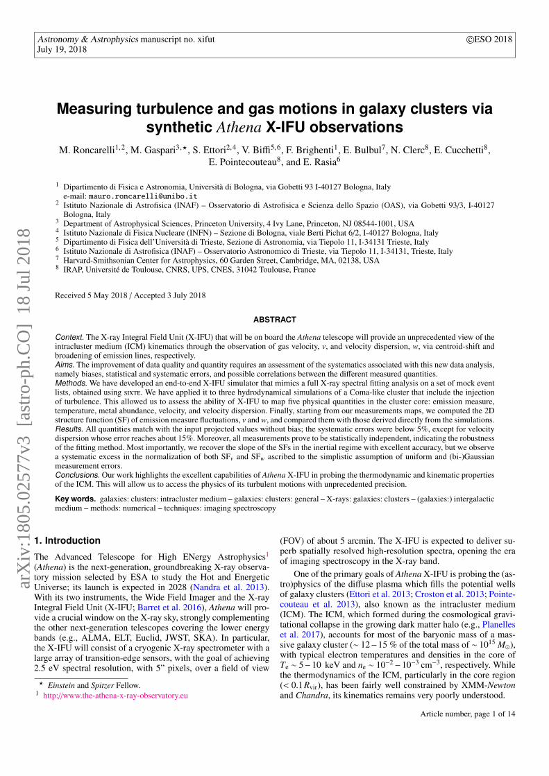
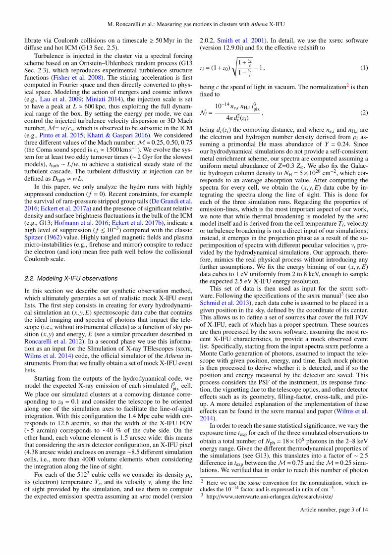
Our three mock event lists undergo a full X-ray analysis. Foreach simulation we divide the X-IFU field of view using theVoronoi tessellation method (Cappellari & Copin 2003) in re-gions containing about 30000 photons each: this translates intoabout 600 pixels. Then we extract the spectra corresponding toeach Voronoi region and, after binning them according to the X-IFU response function, we fit them using xspec (Cash statistics).To account for the effect of vignetting, we consider a differentresponse function for each spectra: this is done by modifying theon-axis X-IFU response function according to the position of thecenter of the Voronoi region, following the same vignetting func-tion as was implemented in sixte. This step leads to a reductionin the effective area of 4% to 8%, depending on the energy, in theexternal regions of the FOV, enough to induce a significant sys-tematic effect if not correctly accounted for. Instead, we neglectthe effect of photon pile-up after verifying that it has a small im-pact in our final mock event lists. Once the response function iscomputed, we fit each spectra through the full 2–8 keV rangeusing xspec assuming a bapec model with five free-parameters:normalization, temperature, metal abundance, redshift, and ve-locity broadening: this procedure is done “blind”, i.e., withoutany a priori knowledge about the input physical conditions; theonly exceptions are the H column density, which we fix to theinput value of NH = 5×1020 cm−2, and the value of z0. We alsopoint out that by adopting a single metallicity value, we are im-plicitly assuming that the abundance ratios of the different ions(O/Fe, Si/Fe, and so on) have solar values. We show in Fig. 1 asketch of the fitting procedure and of its results applied to one ofthe M= 0.75 mock spectra.

The fitting procedure proves to be robust and converges toa result without issues for the majority of the fitted spectra. Inabout 3% of the cases an error occurs in the computation of theconfidence regions;4 this is due both to the complexity of thefitting procedure (i.e., C-stat minimization on a five-parametersspace) and to the intrinsic thermodynamical inhomogeneity ofthe emitting gas. To avoid possible issues we removed thesecases from our analysis.

3. Results

3.1. Intrinsic quantities definitions

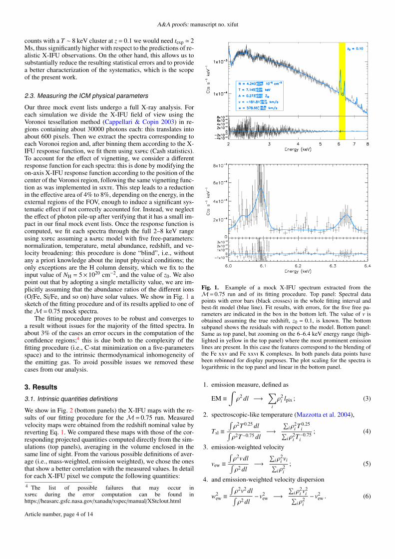
We show in Fig. 2 (bottom panels) the X-IFU maps with the re-sults of our fitting procedure for the M= 0.75 run. Measuredvelocity maps were obtained from the redshift nominal value byreverting Eq. 1. We compared these maps with those of the cor-responding projected quantities computed directly from the sim-ulations (top panels), averaging in the volume enclosed in thesame line of sight. From the various possible definitions of aver-age (i.e., mass-weighted, emission weighted), we chose the onesthat show a better correlation with the measured values. In detailfor each X-IFU pixel we compute the following quantities:4 The list of possible failures that may occur inxspec during the error computation can be found inhttps://heasarc.gsfc.nasa.gov/xanadu/xspec/manual/XStclout.html

Fig. 1. Example of a mock X-IFU spectrum extracted from theM= 0.75 run and of its fitting procedure. Top panel: Spectral datapoints with error bars (black crosses) in the whole fitting interval andbest-fit model (blue line). Fit results, with errors, for the five free pa-rameters are indicated in the box in the bottom left. The value of v isobtained assuming the true redshift, z0 = 0.1, is known. The bottomsubpanel shows the residuals with respect to the model. Bottom panel:Same as top panel, but zooming on the 6–6.4 keV energy range (high-lighted in yellow in the top panel) where the most prominent emissionlines are present. In this case the features correspond to the blending ofthe Fe xxv and Fe xxvi K complexes. In both panels data points havebeen rebinned for display purposes. The plot scaling for the spectra islogarithmic in the top panel and linear in the bottom panel.

1. emission measure, defined as

EM ≡∫ρ2 dl −→

∑i

ρ2i lpix ; (3)

2. spectroscopic-like temperature (Mazzotta et al. 2004),

Tsl ≡

∫ρ2T 0.25 dl∫ρ2T−0.75 dl

−→

∑i ρ

2i T 0.25

i∑i ρ

2i T−0.75

i

; (4)

3. emission-weighted velocity

vew ≡

∫ρ2vdl∫ρ2 dl

−→

∑i ρ

2i vi∑

i ρ2i

; (5)

4. and emission-weighted velocity dispersion

w2ew ≡

∫ρ2v2 dl∫ρ2 dl

− v2ew −→

∑i ρ

2i v2

i∑i ρ

2i

− v2ew . (6)



Fig. 2. X-IFU maps showing input quantities (top panels) vs measured ones (bottom) for the M= 0.75 model. Input quantities are derived directlyfrom the simulation output, considering the average along the line of sight enclosed by the X-IFU pixel (4.38 arcsec wide) and computed with thedefinitions in Eqs.(3)–(6). For measured quantities we show the nominal value derived from the fitting of our synthetic spectra (see text for details)in the corresponding 588 Voronoi regions (≈ 125 arcsec2 each). From left to right: emission measure, gas temperature (spectroscopic-like, in thetop panel), velocity, and velocity dispersion (both emission-weighted, in the top panels).

In the above formulas on the left-hand side we show the ana-lytical definitions with line-of-sight integrals, and on the right-hand side the equivalent numerical definitions with the index irunning through all the cells along the full length of the sim-ulation box (' 1.4 Mpc). While the definition of EM (directlyconnected to the spectrum normalization, as in Eq. 2) and Tslare already widely adopted in X-ray astrophysics, only recentlysome works (see, e.g., Biffi et al. 2013) have proved how the lasttwo quantities correlate with the centroid-shift and line broaden-

ing measurements better than the equivalent mass-weighted val-ues. A visual inspection shows an excellent agreement of bothemission measure and velocity. In particular, it is important tonote that with our mock measurements we are able to recoverthe details of the line-of-sight velocity field with great accuracy.In addition, measured temperature maps show a good agreementwith spectroscopic-like temperature maps. Broadening measure-ments, on the other hand, prove to be the most challenging even



though both the average broadening value and the main featuresof the wew maps are appropriately recovered.

3.2. Biases and uncertainties

In this section we analyze the accuracy of the X-ray mea-surements by comparing them with the input quantities com-puted from the simulations with the definitions of Eqs. 3–6. Inthe following, we will distinguish between biases, i.e., possi-ble systematic offsets in the measurements, and systematic er-rors/uncertainties, i.e., the irreducible scatter between measure-ments and the corresponding theoretical values. For the analysispresented here, the latter values are associated with the limits ofthe assumption of a five-parameter model adopted in our fittingprocedure in the case of ICM mixing. These errors may eventu-ally be reduced by adopting more complicated models (such asallowing multiple ICM components).

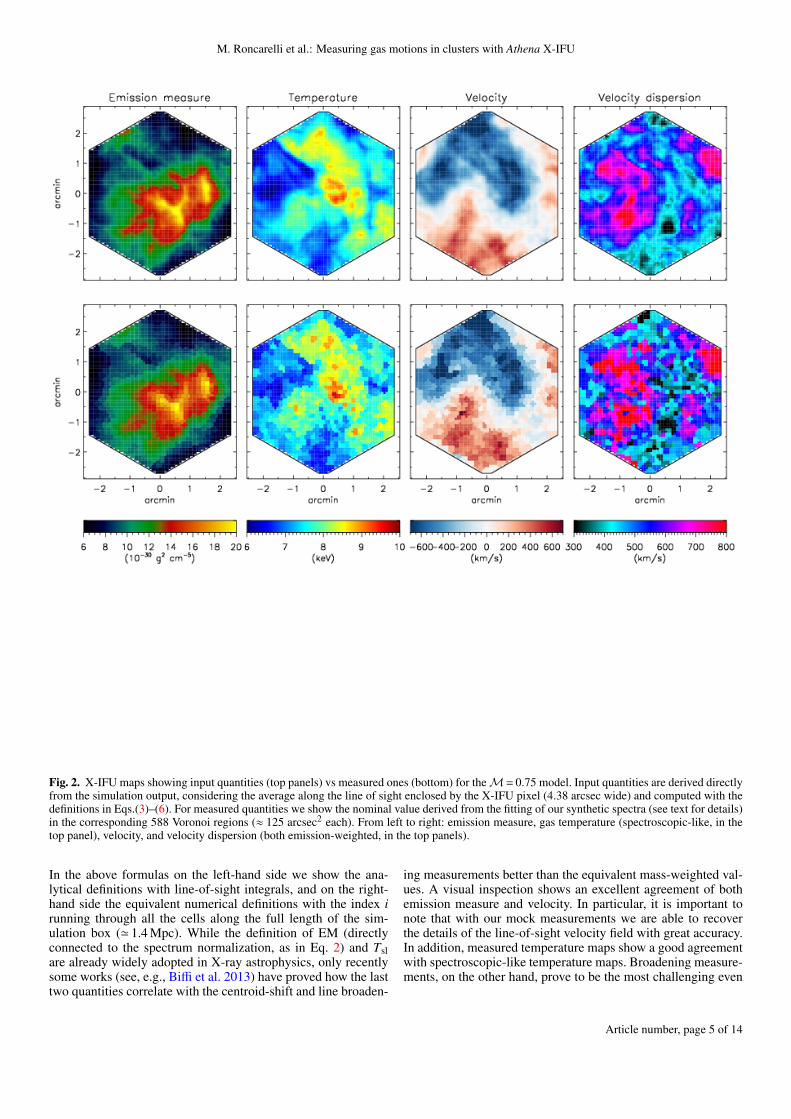
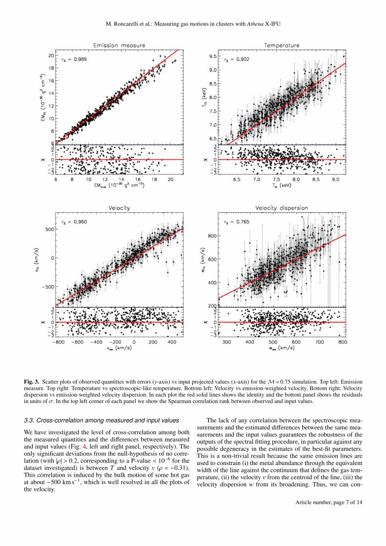
We show in Fig. 3 the relation among the results obtainedfrom the fitting procedure, with errors, and those extracted fromthe simulations for the M= 0.75 model (the red solid lines in-dicate the identity). In Appendix B we show the same plots forthe other two simulations. The values on the x-axes were com-puted by applying the formulas of Eqs. 3–6 directly to the inputhydrodynamical simulation in the volume corresponding to theVoronoi region of the measurements projected along the line ofsight. As expected from Fig. 2, emission measure and velocityshow the most precise measurements. In particular, we point outthat the comparison between the fit result and vew shows no sig-nificant bias even for high values of velocity. Temperature mea-surements show also a good agreement with Tsl, with a small hintof temperature overestimation for the few regions with Tsl< 6.5keV; this may indicate that in the lower temperature regimesthe definition of Tsl provided in Eq. 4, which was optimized forCCDs, might need to be revisited. As expected, the velocity dis-persion measurements also show good agreement with the cor-responding wew, with possibly a hint of overestimation for highwew values. We note that in this case errors in the measurementsmay vary considerably from σw ≈ 40 km s−1 to σw ≈ 100 km s−1.In the top left corner of each plot we show the Spearman correla-tion rank between measured and real quantities. In all cases thecorrelation is extremely high. Indeed, we obtain an almost per-fect correlation (rS ≈ 1) for emission measure and velocity, torS ∼ 0.9 for temperature, and rS ∼ 0.75 for velocity dispersion.This confirms the accuracy of the measurements of the differentphysical quantities.

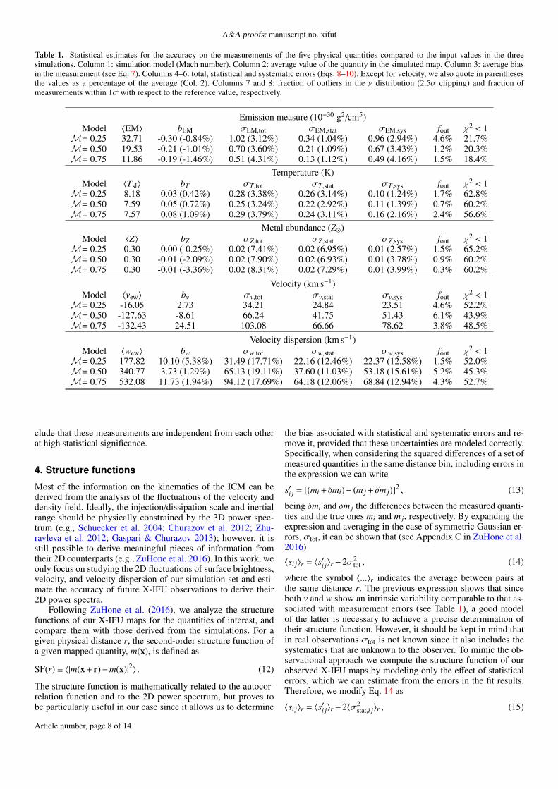
The quantification of these results is shown in Table 1 to-gether with other statistical estimates described and discussed inthe following. All results are reported for the three different sim-ulation setups, and are also related to the metallicity. We definethe average bias (third column) as

b ≡ 〈mi− ti〉 , (7)

where mi and ti are the sets of measured and true projected quan-tities extracted from the simulations (Eqs. 3–6). Remarkably, bi-ases in the measurements are almost negligible for all quanti-ties: this is both an indication of the robustness of the fittingprocedure and of the suitability of the definitions of Eqs. 3–6in representing the observationally derived values. On the otherhand, we verified that mass-weighted quantities are, instead, sig-nificantly different with respect to measured ones, with mass-weighted temperature and velocity dispersion biased high by∼0.2 keV and ∼40 km s−1, respectively. Mass weighted veloc-ities are instead about 30% smaller than observed ones (see alsoBiffi et al. 2013).

In the central columns of the table, we quote the total, statis-tical, and systematic errors of the measured quantities computedin the following way. Total errors are computed as

σ2tot = 〈(mi− ti)2〉 . (8)

Statistical errors are instead derived from the fit errors with thefollowing formula (see details in Appendix A):

σ2stat =

⟨(σ2−σ1)2 +σ1σ2

⟩. (9)

This expression is also appropriate for asymmetric errors, withσ1 and σ2 being the left and right errors, respectively. Thus, inour case it provides a better description with respect to the sim-ple Gaussian error estimates. Systematic errors are then simplyderived as

σ2sys = σ2

tot−σ2stat , (10)

and provide an indication of the expected scatter associated withthe model uncertainty.

For emission measure, the number counts adopted in oursimulations are enough to reduce statistical errors below system-atic ones (∼ 3%). The latter are associated with the X-IFU pointspread function that scatters photons in the areas close to the bor-ders of the Voronoi regions, and would be negligible with a morerealistic exposure time. This also causes the highest EM mea-surements to be slightly underestimated, as it appears in Fig. 3.Most interestingly, we observe that the values of σv,sys increasefor larger Mach numbers, going from 25 km s−1 for M= 0.25 toabout 80 km s−1 for M= 0.75, due to the larger gas mixing. Thesame applies for σw,sys, which grows proportionally with 〈wew〉and with the Mach number, and remains approximately 15% ofthe average value.

In order to evaluate the accuracy of the errors provided byour fitting procedure, for each measurement we compute its nor-malized residual

χ ≡m− tσ1,2

, (11)

being σ1,2 the left and right measurement errors provided by thefit. We then use the distributions of the χ values to determinetwo statistical estimators. First, we identify the outliers by ap-plying a 2.5σ clipping to the different distributions and computeits fraction. Then we compute the fraction of values in the range[−1,1]: this represents the fraction of points within 1σ of the truevalue. The results are listed in the last two columns of Table 1.The outliers fraction for the measurements of EM, T , and Z arecomparable to expected values for the perfectly Gaussian case(1.25%)5. On the other hand, measurement of v and w show asignificant number of outliers: this can happen in regions withlarge gas mixing when a single velocity value is not able to de-scribe the properties of the emission lines.

The values shown in the last column indicate that our fittingprocedure is underestimating the true dispersion of the values ofχ (all values are smaller than 68.8%, expected for perfectly es-timated Gaussian errors). Most notably, this figure is about 45–50% for v and w due both to the presence of outliers and system-atic errors. For T and Z measurements, instead, where statisticalerrors dominate, values are close the expected Gaussian behaviorwith a fraction of measurements within 1σ of ∼60%.5 We verified that the high number of outliers in the EM measurementsfor the M= 0.25 simulation is due to a single region where a shock isoccurring.



Fig. 3. Scatter plots of observed quantities with errors (y-axis) vs input projected values (x-axis) for the M= 0.75 simulation. Top left: Emissionmeasure. Top right: Temperature vs spectroscopic-like temperature. Bottom left: Velocity vs emission-weighted velocity. Bottom right: Velocitydispersion vs emission-weighted velocity dispersion. In each plot the red solid lines shows the identity and the bottom panel shows the residualsin units of σ. In the top left corner of each panel we show the Spearman correlation rank between observed and input values.

3.3. Cross-correlation among measured and input values

We have investigated the level of cross-correlation among boththe measured quantities and the differences between measuredand input values (Fig. 4, left and right panel, respectively). Theonly significant deviations from the null-hypothesis of no corre-lation (with |ρ| > 0.2, corresponding to a P-value < 10−6 for thedataset investigated) is between T and velocity v (ρ = −0.31).This correlation is induced by the bulk motion of some hot gasat about −500 km s−1, which is well resolved in all the plots ofthe velocity.

The lack of any correlation between the spectroscopic mea-surements and the estimated differences between the same mea-surements and the input values guarantees the robustness of theoutputs of the spectral fitting procedure, in particular against anypossible degeneracy in the estimates of the best-fit parameters.This is a non-trivial result because the same emission lines areused to constrain (i) the metal abundance through the equivalentwidth of the line against the continuum that defines the gas tem-perature, (ii) the velocity v from the centroid of the line, (iii) thevelocity dispersion w from its broadening. Thus, we can con-



Table 1. Statistical estimates for the accuracy on the measurements of the five physical quantities compared to the input values in the threesimulations. Column 1: simulation model (Mach number). Column 2: average value of the quantity in the simulated map. Column 3: average biasin the measurement (see Eq. 7). Columns 4–6: total, statistical and systematic errors (Eqs. 8–10). Except for velocity, we also quote in parenthesesthe values as a percentage of the average (Col. 2). Columns 7 and 8: fraction of outliers in the χ distribution (2.5σ clipping) and fraction ofmeasurements within 1σ with respect to the reference value, respectively.

Emission measure (10−30 g2/cm5)Model 〈EM〉 bEM σEM,tot σEM,stat σEM,sys fout χ2 < 1

M= 0.25 32.71 -0.30 (-0.84%) 1.02 (3.12%) 0.34 (1.04%) 0.96 (2.94%) 4.6% 21.7%M= 0.50 19.53 -0.21 (-1.01%) 0.70 (3.60%) 0.21 (1.09%) 0.67 (3.43%) 1.2% 20.3%M= 0.75 11.86 -0.19 (-1.46%) 0.51 (4.31%) 0.13 (1.12%) 0.49 (4.16%) 1.5% 18.4%

Temperature (K)Model 〈Tsl〉 bT σT,tot σT,stat σT,sys fout χ2 < 1

M= 0.25 8.18 0.03 (0.42%) 0.28 (3.38%) 0.26 (3.14%) 0.10 (1.24%) 1.7% 62.8%M= 0.50 7.59 0.05 (0.72%) 0.25 (3.24%) 0.22 (2.92%) 0.11 (1.39%) 0.7% 60.2%M= 0.75 7.57 0.08 (1.09%) 0.29 (3.79%) 0.24 (3.11%) 0.16 (2.16%) 2.4% 56.6%

Metal abundance (Z)Model 〈Z〉 bZ σZ,tot σZ,stat σZ,sys fout χ2 < 1

M= 0.25 0.30 -0.00 (-0.25%) 0.02 (7.41%) 0.02 (6.95%) 0.01 (2.57%) 1.5% 65.2%M= 0.50 0.30 -0.01 (-2.09%) 0.02 (7.90%) 0.02 (6.93%) 0.01 (3.78%) 0.9% 60.2%M= 0.75 0.30 -0.01 (-3.36%) 0.02 (8.31%) 0.02 (7.29%) 0.01 (3.99%) 0.3% 60.2%

Velocity (km s−1)Model 〈vew〉 bv σv,tot σv,stat σv,sys fout χ2 < 1

M= 0.25 -16.05 2.73 34.21 24.84 23.51 4.6% 52.2%M= 0.50 -127.63 -8.61 66.24 41.75 51.43 6.1% 43.9%M= 0.75 -132.43 24.51 103.08 66.66 78.62 3.8% 48.5%

Velocity dispersion (km s−1)Model 〈wew〉 bw σw,tot σw,stat σw,sys fout χ2 < 1

M= 0.25 177.82 10.10 (5.38%) 31.49 (17.71%) 22.16 (12.46%) 22.37 (12.58%) 1.5% 52.0%M= 0.50 340.77 3.73 (1.29%) 65.13 (19.11%) 37.60 (11.03%) 53.18 (15.61%) 5.2% 45.3%M= 0.75 532.08 11.73 (1.94%) 94.12 (17.69%) 64.18 (12.06%) 68.84 (12.94%) 4.3% 52.7%

clude that these measurements are independent from each otherat high statistical significance.

4. Structure functions

Most of the information on the kinematics of the ICM can bederived from the analysis of the fluctuations of the velocity anddensity field. Ideally, the injection/dissipation scale and inertialrange should be physically constrained by the 3D power spec-trum (e.g., Schuecker et al. 2004; Churazov et al. 2012; Zhu-ravleva et al. 2012; Gaspari & Churazov 2013); however, it isstill possible to derive meaningful pieces of information fromtheir 2D counterparts (e.g., ZuHone et al. 2016). In this work, weonly focus on studying the 2D fluctuations of surface brightness,velocity, and velocity dispersion of our simulation set and esti-mate the accuracy of future X-IFU observations to derive their2D power spectra.

Following ZuHone et al. (2016), we analyze the structurefunctions of our X-IFU maps for the quantities of interest, andcompare them with those derived from the simulations. For agiven physical distance r, the second-order structure function ofa given mapped quantity, m(x), is defined as

SF(r) ≡ 〈|m(x + r)−m(x)|2〉 . (12)

The structure function is mathematically related to the autocor-relation function and to the 2D power spectrum, but proves tobe particularly useful in our case since it allows us to determine

the bias associated with statistical and systematic errors and re-move it, provided that these uncertainties are modeled correctly.Specifically, when considering the squared differences of a set ofmeasured quantities in the same distance bin, including errors inthe expression we can write

s′i j = [(mi +δmi)− (m j +δm j)]2 , (13)

being δmi and δm j the differences between the measured quanti-ties and the true ones mi and m j, respectively. By expanding theexpression and averaging in the case of symmetric Gaussian er-rors, σtot, it can be shown that (see Appendix C in ZuHone et al.2016)

〈si j〉r = 〈s′i j〉r −2σ2tot , (14)

where the symbol 〈...〉r indicates the average between pairs atthe same distance r. The previous expression shows that sinceboth v and w show an intrinsic variability comparable to that as-sociated with measurement errors (see Table 1), a good modelof the latter is necessary to achieve a precise determination oftheir structure function. However, it should be kept in mind thatin real observations σtot is not known since it also includes thesystematics that are unknown to the observer. To mimic the ob-servational approach we compute the structure function of ourobserved X-IFU maps by modeling only the effect of statisticalerrors, which we can estimate from the errors in the fit results.Therefore, we modify Eq. 14 as

〈si j〉r = 〈s′i j〉r −2〈σ2stat,i j〉r , (15)



Fig. 4. Left panel: Corner plot and heat map for the measured best-fit spectral quantities in the case of M= 0.75. The distributions (median, 1st and3rd quartiles) and the correlations among the measured quantities are shown. The heat map is color-coded and indicates the level of correlationsamong the same quantities. Right panel: Same as left panel, but evaluated using the differences between measured and reference values.

where the last term represents the average of the statistical vari-ance of the set of points at the same distance r. Since in ourresults we have non-symmetric errors, each value of σ2

stat,i j isderived from the left-hand and right-hand error as in Eq. 9.

Considering all of the above, we derive the best observationalestimate of the (2D) structure functions of surface brightnessfluctuations δ, v, and w, respectively, with the following formu-las:

SFδ(r) = 〈|δ(x + r)−δ(x)|2−2σ2δ,stat〉 , (16)

SFv(r) = 〈|v(x + r)− v(x)|2−2σ2v,stat〉 , (17)

and

SFw(r) = 〈|w(x + r)−w(x)|2−2σ2w,stat〉 . (18)

The quantity δ that appears in Eq. 16 is defined as

δ(x) ≡EM(x)〈EM(r)〉

−1 . (19)

The corresponding statistical error σδ,stat =σEM,stat/〈EM(r)〉, be-ing 〈EM(r)〉 the average surface brightness of the points at thesame distance r from the peak of the emission measure map; thisconversion allows us to study the surface brightness fluctuationswith respect to the average profile. We note that the SFv (at larger) is tied to the variance of the turbulence field (i.e., specific ki-netic energy), while the SFw (line broadening) is linked to thevariance of the turbulent velocity, which can be interpreted as ameasure of turbulence intermittency.

It is important to note that the region covered by our X-IFUsimulations, i.e., the core of our simulated cluster, allows us toestimate fluctuations up to a maximum distance of 350 kpc. Inorder to obtain a complete representation of the SFs over thefull cluster volume (fully capturing the injection scale) we would

need to enlarge the total area by a factor of ∼10, with multipleX-IFU pointings, which is beyond the scope of this work. In ad-dition, the SFs measured in the core can significantly vary fromthe global SFs (which describe the full physical cascade6) be-cause of the cosmic variance and related stochastic nature of theturbulent eddies along a given line of sight. As a reference, weverified that the logarithmic scatter in the amplitude of the SFsdue to the different line-of-sight projection in our simulations is∆ ALog ' 0.10−0.15 (at r < 100 kpc).

The comparison between observationally derived and inputSFδ, SFv, and SFw is shown in Fig. 5. To understand the effectof the statistical error correction, we also show (open circles) thesame results neglecting the −2σ2

stat terms. The structure functionof the emission measure fluctuations δ is recovered almost per-fectly, with only a minor difference for the M= 0.5 simulation.This is expected given the high correlation between measuredand input quantities (see the discussion in Section 3.2) and thesmall measurement errors. The general shape of the structurefunction of the velocity field is also recovered, with the threephysical models clearly distinguishable. However, measured val-ues show a non-negligible overestimate (about 5–10%); this canbe partially explained as systematic errors that are not accountedfor in our computation and that would introduce a −2σ2

v,sys termin the equation. We also point out that the modeling of error sub-traction described by Eq. 15 works under the hypothesis of bothuniform and Gaussian errors, which is not completely true due tothe presence of a non-negligible number of outliers, as discussedin Section 3.2. This means that in order to achieve a more robustcharacterization of SFv, a more accurate error model is required.All these considerations also apply to SFw, with a significantlylarger overestimate associated with the error subtraction.

6 We verified that taking multiple projections and a large cube repro-duces the proper Kolmogorov 2D SFv with 5/3 slope and gradual flat-tening only at several 100 kpc near the injection scale.



Fig. 5. Second-order 2D structure functions of emission measure fluc-tuations (top), velocity (middle), and velocity dispersion (bottom) asa function of distance for the three M = (0.25,0.5,0.75) simulations(green, blue, and red, respectively). In each plot the measured SFs de-rived from our simulated X-IFU fields (filled dots with error bars) iscompared to those of δ, vew, and wew (see definitions in Eqs. 3, 5, and6) derived directly from the hydrodynamical simulations in the samefield of view (solid lines). Error bars represent the error on the meancomputed with 100 bootstrap samplings (in most cases smaller than thedot size). Open circles indicate the values of the measured SFs withoutthe statistical error subtraction (see Eqs. 17 and 18). The FOV coversonly a small fraction of the cluster, namely the core region.

We analyze the impact of these systematics in determiningthe properties of the 2D power spectrum, P2D, of the differentquantities. As pointed out in ZuHone et al. (2016), if we as-sume a power-law form of the power spectrum in the inertialrange (i.e., below the injection scale), P2D(k) ∝ kα, then the cor-responding SF scales as rγ, with γ = −(α+ 2). Therefore, we fitthe SFs of Fig. 5 using

SF(r) = A(

rr0

)γ, (20)

with r0 fixed to 100 kpc, while A and γ are left as free parame-ters. We compute the fit in the interval 30–120 kpc to ensure thatin all cases we have functions that increase with r and avoid theflattening due to the large-scale plateau. Finally, by comparingthe resulting best-fit values obtained from our mock measure-ments with those obtained directly from the projected simulationquantities, we are able to estimate the impact of the systematicsin the structure function on the slope and normalization of theSF itself and, consequently, of their P2D.

Table 2. From top to bottom: Normalization and slopes of the struc-ture functions, SF(r), of emission measure fluctuations, velocity, andvelocity dispersion, for the three simulations with M= (0.25,0.5,0.75).Column 1: simulation model (Mach number). Columns 2 and 3: normal-ization derived from simulations and from measured quantities, respec-tively. Units are shown in parenthesis. Columns 4 and 5: same as Cols.2 and 3, respectively, but for the slope. The fitting range is 30–120 kpc.

Emission measure fluctuations (10−3)Model Aδ,sim Aδ,meas γδ,sim γδ,meas

M= 0.25 9.15 8.00 1.17 1.20M= 0.50 31.85 27.56 1.09 1.13M= 0.75 40.29 38.57 0.96 0.93

Velocity (104 km2/s2)Model Av,sim Av,meas γv,sim γv,meas

M= 0.25 2.19 2.66 1.56 1.63M= 0.50 7.00 9.49 1.45 1.41M= 0.75 9.32 10.76 1.33 1.36

Velocity dispersion (104 km2/s2)Model Aw,sim Aw,meas γw,sim γw,meas

M= 0.25 0.40 0.75 0.94 0.84M= 0.50 0.59 0.85 0.46 0.41M= 0.75 1.72 3.12 0.87 0.75

We show the results of the fit in Table 2. It is clear that theonly significant impact of the systematics in our SFs is in thenormalization estimate. The value of Av,meas exceeds the inputvalue by 15–30%, while for Aw,meas it can be almost doubled.On the other hand, the slopes of the initial structure functionsare correctly recovered in all cases, with maximum differencesbetween input and measured values of ∼ 0.1.7 This confirms thatthe systematics in the SFs measurements are induced by an un-derestimation of the −2σ2

stat, which boosts our measurements buthas a minor impact on the slope.

5. Summary and conclusions

We have developed, for the first time, an end-to-end mock X-rayanalysis pipeline that mimics future Athena X-IFU observations.Our goal was to quantify possible systematics that may arise inthe measurements of the main projected physical properties ofthe ICM, emission measure, temperature, and metallicity; mostnotably, the two key quantities that will be made available viahigh-resolution spectroscopic imaging are the line-of-sight ve-locity v derived from the centroid shift of the emission lines, andthe velocity dispersion w derived from their broadening. In thiswork we applied our pipeline to a set of three hydrodynamicalsimulations (Gaspari & Churazov 2013; Gaspari et al. 2014) thatmodel the injection of turbulence in a Coma-like galaxy clus-ter, assuming different Mach numbers M = (0.25,0.5,0.75). Us-ing the sixte software, we obtained three simulated event liststhat represent X-IFU observations in ideal conditions (i.e., withenough photons not to be limited by statistics) and then applieda realistic observational pipeline to measure and map the quanti-ties mentioned above. This was done by fitting about 600 spectrafor each X-IFU FOV, allowing a comparison with the equiva-

7 The SFv slopes for the M= 0.5 and M= 0.75 runs are somewhatsmaller than the Kolmogorov slope (γ = 5/3), which characterizes thesubsonic turbulence stirring the whole cluster. We verified that this isdue to the variance associated with the limited FOV.



lent input projected quantities extracted directly from the hydro-dynamical simulations. Finally, we computed the 2D structurefunctions of the three main quantities that can be used to describethe properties of turbulence, namely emission measure fluctua-tions v and w, and verified our ability to recover their input slopeand normalization.

Our main results can be summarized as follows:

i) The centroid shift and line broadening measured by fittingthe X-IFU spectra correspond well to the emission-weightedvelocity and velocity dispersion (see Eqs. 5 and 6, respec-tively) computed in the same region. The temperature is ap-propriately described by the spectroscopic-like temperature(Eq. 4, Mazzotta et al. 2004);

ii) No significant bias is found in the measurement of the fivephysical quantities investigated in our analysis. The ex-pected systematic uncertainties (listed in Table 1) due tothe modeling assumed in the fitting procedure are smallerthan 5% for all quantities, except for the broadening whereit reaches about 15%;

iii) The physical quantities measured with our fitting procedureand their differences with the input projected values proveto be independent from each other at high statistical signifi-cance. This corroborates the accuracy of the current spectralfitting approach. Improvements on the fitting errors and tothe residual systematic can be considered, for example us-ing optimal binning or other fitting methods;

iv) The overall shape of the 2D structure functions of emissionmeasure fluctuations, velocity, and velocity dispersion is re-covered well. However, we observe an excess of 15–30%and of 40–80% in measurement of the normalization of SFvand SFw, respectively: this is due to the limitations of thesimplistic assumption on the error shapes;

v) We verified that these discrepancies do not affect the abil-ity to measure the slope of the 2D structure functions of allquantities and thus of their 2D power spectrum. In all casesthe input slope is recovered at high precision, with differ-ences smaller than 0.1.

Our work highlights the unprecedented X-IFU capability ofprobing the thermodynamics and kinematics properties of theICM, and of deriving the properties of its turbulent motions. Inthe near future we plan to extend our simulations to a largerFOV to better capture the injection scale of turbulence, and torun our simulator over a set of hydrodynamical simulations in acosmological environment to estimate the cosmic variance asso-ciated with the turbulence power spectrum in a large-scale struc-ture scenario. In addition, in the framework of Athena sciencegoals, it will be interesting to test the robustness of our fittingprocedures using models that do not assume solar ratios for themetallicities, i.e., increasing the number of free parameters tomeasure the abundance of the various elements independently.Acknowledgements. This work has been completed despite the shameful situa-tion of the Italian research system, worsened by an entire decade of severe cutsto the fundings of public universities and research institutes (see, e.g., Abbott2006, 2016, 2018). This has caused a whole generation of valuable researchers,in all fields, to struggle in poor working conditions with little hope of achievingdecent employment contracts and permanent positions, resulting in obvious dif-ficulties in the planning of future research activities, and in open violation of theEuropean Charter for Researchers8.We acknowledge support by the ASI (Italian Space Agency) through Contractno. 2015-046-R.0. M.R. also acknowledges the financial contribution from ASIagreement no. I/023/12/0 “Attività relative alla fase B2/C per la missione Eu-clid”. M.G. is supported by NASA through Einstein Postdoctoral FellowshipAward Number PF5-160137 issued by the Chandra X-ray Observatory Center,

8 https://euraxess.ec.europa.eu/jobs/charter

which is operated by the SAO for and on behalf of NASA under contract NAS8-03060. Support for this work was also provided by Chandra GO7-18121X.S.E. acknowledges financial contribution from contracts NARO15 ASI-INAFI/037/12/0, ASI 2015-046-R.0, and ASI-INAF no. 2017-14-H.0. The FLASH codewas in part developed by the DOE NNSA-ASC OASCR Flash center at the Uni-versity of Chicago. HPC resources were in part provided by the NASA HEC Pro-gram (SMD-17-7251). E.R. acknowledges the ExaNeSt and Euro Exa projects,funded by the European Union’s Horizon 2020 research and innovation programunder grant agreement No. 671553 and No. 754337 and financial contributionfrom ASI-INAF agreement no. 2017-14-H.0.We thank the anonymous referee for providing useful comments. We are gratefulto S. Borgani, K. Dolag, M. Gitti, G. Lanzuisi, and P. Peille for insightful discus-sions. We also thank the sixte development team for their help and support.

ReferencesAbbott, A. 2006, Nat, 440, 264Abbott, A. 2016, Nat, 540, 324Abbott, A. 2018, Nat, 554, 411Anders, E. & Grevesse, N. 1989, Geochim. Cosmochim. Acta, 53, 197Barret, D., Lam Trong, T., den Herder, J.-W., et al. 2016, in Proc. SPIE, Vol.

9905, Space Telescopes and Instrumentation 2016: Ultraviolet to GammaRay, 99052F

Beresnyak, A. & Miniati, F. 2016, ApJ, 817, 127Biffi, V., Borgani, S., Murante, G., et al. 2016, ApJ, 827, 112Biffi, V., Dolag, K., & Böhringer, H. 2013, MNRAS, 428, 1395Bonafede, A., Brüggen, M., Rafferty, D., et al. 2018, MN-

RAS[arXiv:1805.00473]Brunetti, G., Setti, G., Feretti, L., & Giovannini, G. 2001, MNRAS, 320, 365Bulbul, G. E., Smith, R. K., Foster, A., et al. 2012, ApJ, 747, 32Cappellari, M. & Copin, Y. 2003, MNRAS, 342, 345Cho, J., Vishniac, E. T., Beresnyak, A., Lazarian, A., & Ryu, D. 2009, ApJ, 693,

1449Churazov, E., Forman, W., Jones, C., Sunyaev, R., & Böhringer, H. 2004, MN-

RAS, 347, 29Churazov, E., Vikhlinin, A., Zhuravleva, I., et al. 2012, MNRAS, 421, 1123Croston, J. H., Sanders, J. S., Heinz, S., et al. 2013, ArXiv e-prints

[arXiv:1306.2323]De Grandi, S., Eckert, D., Molendi, S., et al. 2016, A&A, 592, A154Dolag, K., Vazza, F., Brunetti, G., & Tormen, G. 2005, MNRAS, 364, 753Eckert, D., Gaspari, M., Owers, M. S., et al. 2017a, A&A, 605, A25Eckert, D., Gaspari, M., Vazza, F., et al. 2017b, ApJ, 843, L29Eckert, D., Ghirardini, V., Ettori, S., et al. 2018, ArXiv e-prints

[arXiv:1805.00034]Eckert, D., Roncarelli, M., Ettori, S., et al. 2015, MNRAS, 447, 2198Ettori, S., Pratt, G. W., de Plaa, J., et al. 2013, ArXiv e-prints

[arXiv:1306.2322]Fisher, R. T., Kadanoff, L. P., Lamb, D. Q., et al. 2008, IBM J. Res. & Dev., 52,

127Gaspari, M. 2015, MNRAS, 451, L60Gaspari, M. & Churazov, E. 2013, A&A, 559, A78Gaspari, M., Churazov, E., Nagai, D., Lau, E. T., & Zhuravleva, I. 2014, A&A,

569, A67Gaspari, M., McDonald, M., Hamer, S. L., et al. 2018, ApJ, 854, 167Gaspari, M. & Sadowski, A. 2017, ApJ, 837, 149Hitomi Collaboration, Aharonian, F., Akamatsu, H., et al. 2016, Nat, 535, 117Hitomi Collaboration, Aharonian, F., Akamatsu, H., et al. 2018, PASJ, 70, 9Hofmann, F., Sanders, J. S., Nandra, K., Clerc, N., & Gaspari, M. 2016, A&A,

585Inogamov, N. A. & Sunyaev, R. A. 2003, Astronomy Letters, 29, 791Khatri, R. & Gaspari, M. 2016, MNRAS, 463, 655Lau, E. T., Gaspari, M., Nagai, D., & Coppi, P. 2017, ApJ, 849, 54Lau, E. T., Kravtsov, A. V., & Nagai, D. 2009, ApJ, 705, 1129Mazzotta, P., Rasia, E., Moscardini, L., & Tormen, G. 2004, MNRAS, 354, 10Miniati, F. 2014, ApJ, 782, 21Nandra, K., Barret, D., Barcons, X., et al. 2013, ArXiv e-prints

[arXiv:1306.2307]Ogorzalek, A., Zhuravleva, I., Allen, S. W., et al. 2017, MNRAS, 472, 1659Petrosian, V. 2001, ApJ, 557, 560Piffaretti, R. & Valdarnini, R. 2008, A&A, 491, 71Pinto, C., Sanders, J. S., Werner, N., et al. 2015, A&A, 575, A38Planelles, S., Fabjan, D., Borgani, S., et al. 2017, MNRAS, 467, 3827Pointecouteau, E., Reiprich, T. H., Adami, C., et al. 2013, ArXiv e-prints

[arXiv:1306.2319]Rasia, E., Meneghetti, M., Martino, R., et al. 2012, New Journal of Physics, 14,

055018Roncarelli, M., Cappelluti, N., Borgani, S., Branchini, E., & Moscardini, L.

2012, MNRAS, 424, 1012


https://euraxess.ec.europa.eu/jobs/charter


Roncarelli, M., Ettori, S., Borgani, S., et al. 2013, MNRAS, 432, 3030Roncarelli, M., Ettori, S., Dolag, K., et al. 2006, MNRAS, 373, 1339Sanders, J. S. & Fabian, A. C. 2013, MNRAS, 429, 2727Sanders, J. S., Fabian, A. C., Frank, K. A., Peterson, J. R., & Russell, H. R. 2010,

MNRAS, 402, 127Santos-Lima, R., de Gouveia Dal Pino, E. M., Kowal, G., et al. 2014, ApJ, 781,

84Schmid, C., Smith, R., & Wilms, J. 2013, SIMPUT - A File Format for Simula-

tion Input, Tech. report, HEASARC, Cambridge (MA)Schuecker, P., Finoguenov, A., Miniati, F., Böhringer, H., & Briel, U. G. 2004,

A&A, 426, 387Shi, X., Komatsu, E., Nagai, D., & Lau, E. T. 2016, MNRAS, 455, 2936Smith, R. K., Brickhouse, N. S., Liedahl, D. A., & Raymond, J. C. 2001, ApJ,

556, L91Spitzer, L. 1962, Physics of Fully Ionized GasesVazza, F., Brunetti, G., Gheller, C., Brunino, R., & Brüggen, M. 2011a, A&A,

529, A17Vazza, F., Roncarelli, M., Ettori, S., & Dolag, K. 2011b, MNRAS, 413, 2305Voit, G. M. 2018, ArXiv e-prints [arXiv:1803.06036]Walker, S. A., Sanders, J. S., & Fabian, A. C. 2015, MNRAS, 453, 3699Wallis, K. F. 2014, Statistical Science, 29, 106Wilms, J., Brand, T., Barret, D., et al. 2014, in Proc. SPIE, Vol. 9144, Space

Telescopes and Instrumentation 2014: Ultraviolet to Gamma Ray, 91445XZhuravleva, I., Churazov, E., Arévalo, P., et al. 2015, MNRAS, 450, 4184Zhuravleva, I., Churazov, E., Kravtsov, A., & Sunyaev, R. 2012, MNRAS, 422,

2712ZuHone, J. A., Markevitch, M., & Zhuravleva, I. 2016, ApJ, 817, 110

Appendix A: Statistical uncertainty withasymmetric errors

The calculation of the expected variance of the difference be-tween true and measured quantities in the case of asymmetricerrors must take into account the properties of the split-normal(or double Gaussian) distribution (see, e.g., Wallis 2014). Specif-ically, we consider that for a given measurement µ+σ2

−σ1the poste-

rior probability of the true value X is described by the distribu-tion

f (X) =

A exp

[−

(X−µ)2

2σ21

]for X ≤ µ

A exp[−

(X−µ)2

2σ22

]for X ≥ µ

, (A.1)

where A =(√

2π(σ1 +σ2)/2)−1

. In this case µ represents themode of the distribution, i.e., the nominal value of the measure-ment. It is possible to show that the mean and the variance of thedistributions are

E(X) = µ+

√2π

(σ1−σ2) (A.2)

and

V(X) =

(1−

2π

)(σ1−σ2)2 +σ1σ2 , (A.3)

respectively. Since we are interested in the expected dispersionwith respect to µ, which we consider as our reference value forthe measurements, we can derive it from the last two equations,

σ2µ(X) = V(X) + [E(X)−µ]2 = (σ2−σ1)2 +σ1σ2 , (A.4)

which we adopt as a definition of σ2stat in Eq. 9.

Appendix B: Additional plots

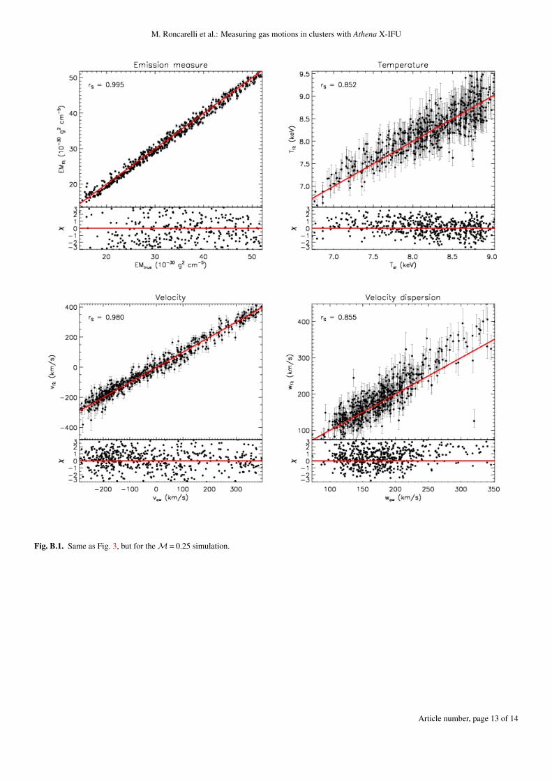
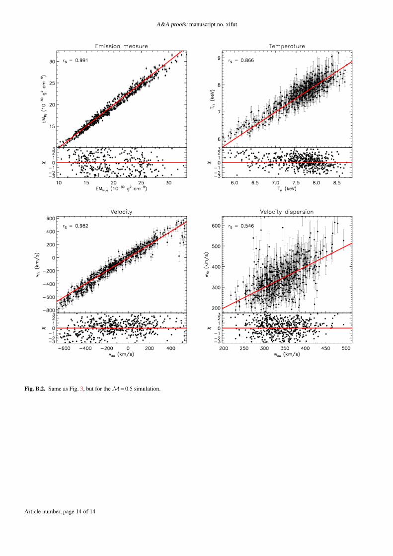
In this Appendix, as a further reference, we show the plot inFig. 3 for the other two simulations. The plot for the M= 0.25and M= 0.5 simulations are shown in Fig. B.1 and Fig. B.2,respectively.



Fig. B.1. Same as Fig. 3, but for the M= 0.25 simulation.



Fig. B.2. Same as Fig. 3, but for the M= 0.5 simulation.


Documents

Measuring turbulence and gas motions in galaxy clusters