Embed Size (px)
Citation preview

arX
iv:1
402.
1548
v1 [
astr
o-ph
.IM
] 7
Feb
201
4Publications of the Astronomical Society of Australia (PASA)© Astronomical Society of Australia 2014; published by Cambridge University Press.doi: 10.1017/pas.2014.xxx.
Measuring Noise Temperatures of Phased-Array Antennas
for Astronomy at CSIRO
A. P. Chippendale1,3, D. B. Hayman2 and S. G. Hay21CSIRO Astronomy and Space Science, PO Box 76, Epping, NSW 1710, Australia2CSIRO Computational Informatics, PO Box 76, Epping, NSW 1710, Australia3Email: [email protected]
Abstract
We describe the development of a noise-temperature testing capability for phased-array antennas operatingin receive mode from 0.7 GHz to 1.8 GHz. Sampled voltages from each array port were recorded digitallyas the zenith-pointing array under test was presented with three scenes: (1) a large microwave absorber atambient temperature, (2) the unobstructed radio sky, and (3) broadband noise transmitted from a referenceantenna centred over and pointed at the array under test. The recorded voltages were processed in softwareto calculate the beam equivalent noise temperature for a maximum signal-to-noise ratio beam steered at thezenith. We introduced the reference-antenna measurement to make noise measurements with reproducible,well-defined beams directed at the zenith and thereby at the centre of the absorber target. We applied adetailed model of cosmic and atmospheric contributions to the radio sky emission that we used as a noise-temperature reference. We also present a comprehensive analysis of measurement uncertainty includingrandom and systematic effects. The key systematic effect was due to uncertainty in the beamformed antennapattern and how efficiently it illuminates the absorber load. We achieved a combined uncertainty as low as4 K for a 40 K measurement of beam equivalent noise temperature. The measurement and analysis techniquesdescribed in this paper were pursued to support noise-performance verification of prototype phased-arrayfeeds for the Australian Square Kilometre Array Pathfinder telescope.
Keywords: Astronomical instrumentation, methods and techniques
1 INTRODUCTION
Developing low-noise, wideband, receive-only array an-tennas is crucial to delivering the Square Kilometre Ar-ray (SKA) telescope (Dewdney et al. 2009). Using aper-ture arrays and phased-array feeds (PAFs) allows moreinformation to be collected from more of the sky inparallel. This increases instantaneous field of view, in-creases survey speed, and allows more agile observingstrategies as electronic beam steering can be immediate.Array antennas enable telescope designers to spend
more money on digital signal processing and less on me-chanical signal processing via telescope dishes for a fixedperformance goal. This trade-off becomes more effectivewith time because digital signal-processing is becomingexponentially cheaper while the cost of dishes is not.The SKA project explored this trade-off (Schilizzi et al.2007; Chippendale et al. 2007; Alexander et al. 2007)and settled on significant deployments of both PAFsand aperture arrays in SKA phase 1 (Dewdney 2013).Important to the development of low-noise array
antennas is the ability to make accurate and repro-
Figure 1. Absorber rolled over array under test at Parkes.
ducible measurements of their noise performance af-ter beamforming. A common approach for measur-ing array noise temperature is to apply the same Y-
1
2 A. P. Chippendale, D. B. Hayman and S. G. Hay
factor method used for single-antenna astronomy re-ceivers (Sinclair & Gough 1991) to the beamformedpower from an array antenna (Woestenburg & Dijkstra2003). The Y-factor is the ratio of beamformed powerbetween observations of “hot” and “cold” loads. Atdecimetre wavelengths, the hot load is often providedby microwave absorber at ambient temperature (Figure1) and the cold load by cosmic radio emission from theunobstructed sky.A number of groups have reported recent develop-
ments in test facilities and measurement techniques forlow-noise arrays. Some experiments have positioned theabsorber at the end of a tapered metal funnel or groundshield (Warnick 2009; Woestenburg et al. 2011). Othershave used more open structures, like CSIRO’s in Fig-ure 1, to support the absorber over the array under test(Woestenburg et al. 2012).Previous work with a ground shield has indi-
cated small differences between measured systemnoise temperatures with and without the shield(Woestenburg et al. 2011). The differences generally de-crease with increase in the beamformed directivity ofthe array under test. At low directivity, where the shieldis significant, the shield only partly decreased the effectof the terrestrial environment.In this paper we describe CSIRO’s development of
an aperture-array noise-temperature testing capabilityat Parkes Observatory. We develop a Y-factor approachsimilar to (Woestenburg et al. 2012) but introduce areference-antenna (Figure 2) measurement to constrainthe pointing of the beam towards the zenith and there-fore the centre of the absorber.
2 PARKES TEST FACILITY
The aperture-array test facility at CSIRO Parkes Ob-servatory (-3259’56”S, 14816’3”E) uses a large rectan-gular microwave absorber supported by an open frame.Figure 1 shows that this absorber may be easily rolledover or away from the array under test via a wheel-on-track arrangement. The aperture-array test pad isserviced by power, radio-frequency (RF) cabling, and adigital receiver and beamformer in a neighbouring hut.A nearby 12 m parabolic reflector has been used to
test arrays at its focal plane using the same digital re-ceiver as the aperture-array measurements. Correlatedmeasurements against signals from the 64 m Parkes ra-dio telescope have also been used to boost testing capa-bility in signal-to-noise ratio and the ability to measurephase (Chippendale et al. 2010). The 64 m dish is lo-cated approximately 400 m west of the 12 m dish andaperture array test pad.
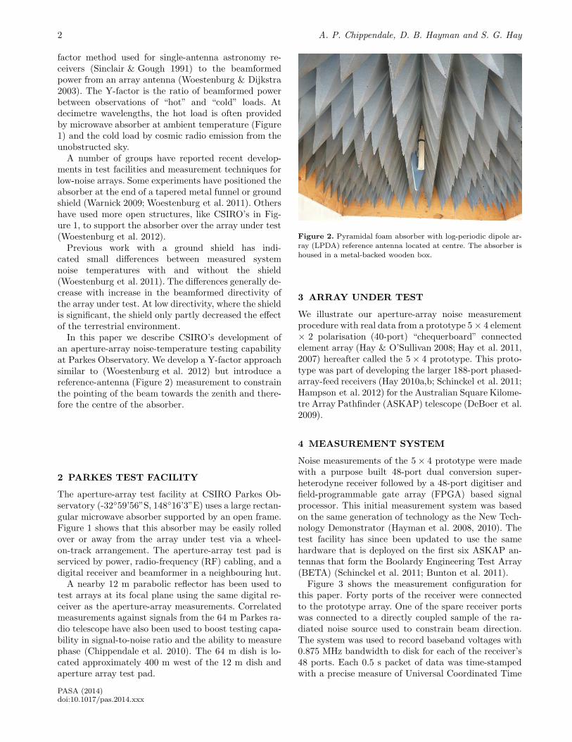
Figure 2. Pyramidal foam absorber with log-periodic dipole ar-ray (LPDA) reference antenna located at centre. The absorber ishoused in a metal-backed wooden box.
3 ARRAY UNDER TEST
We illustrate our aperture-array noise measurementprocedure with real data from a prototype 5× 4 element× 2 polarisation (40-port) “chequerboard” connectedelement array (Hay & O’Sullivan 2008; Hay et al. 2011,2007) hereafter called the 5× 4 prototype. This proto-type was part of developing the larger 188-port phased-array-feed receivers (Hay 2010a,b; Schinckel et al. 2011;Hampson et al. 2012) for the Australian Square Kilome-tre Array Pathfinder (ASKAP) telescope (DeBoer et al.2009).
4 MEASUREMENT SYSTEM
Noise measurements of the 5× 4 prototype were madewith a purpose built 48-port dual conversion super-heterodyne receiver followed by a 48-port digitiser andfield-programmable gate array (FPGA) based signalprocessor. This initial measurement system was basedon the same generation of technology as the New Tech-nology Demonstrator (Hayman et al. 2008, 2010). Thetest facility has since been updated to use the samehardware that is deployed on the first six ASKAP an-tennas that form the Boolardy Engineering Test Array(BETA) (Schinckel et al. 2011; Bunton et al. 2011).Figure 3 shows the measurement configuration for
this paper. Forty ports of the receiver were connectedto the prototype array. One of the spare receiver portswas connected to a directly coupled sample of the ra-diated noise source used to constrain beam direction.The system was used to record baseband voltages with0.875 MHz bandwidth to disk for each of the receiver’s48 ports. Each 0.5 s packet of data was time-stampedwith a precise measure of Universal Coordinated Time
PASA (2014)doi:10.1017/pas.2014.xxx

Measuring Noise Temperatures of Array Antennas 3
LNA
RF BPF
Variable LO3184-4284 MHz
Fixed LO2414 MHz
LPDA
Microwave Absorber
Noise
Reference Noise d(t)
40 Array Ports x(t)
∆f 26MHzfo 70MHz
32
48 ADCs56 MS/s 10 bit CABB DSP Board
48 x 32 Channel PFB
10 G
E48
x 0
.875
MH
z C
hann
els
0.875MHz/Channel
DataRecordingComputer
12 TBRAIDDisk Array
Source
Figure 3. Block diagram of beamformed noise performance measurement setup for a 5× 4 prototype phased-array antenna.
(UTC) from an atomic clock reference. Although thesystem is capable of online beamforming, offline beam-forming on recorded data allowed exploration of dif-ferent beamforming and radio-frequency interference(RFI) removal strategies.Each LNA output was filtered, amplified, up-
converted to an intermediate frequency (IF) of2.484 GHz, and then down-converted to an IF of70 MHz. The 26 MHz bandwidth IF at 70 MHz was sam-pled at 56 MSPS then separated into 32× 0.875 MHzchannels by a digital polyphase filter bank (PFB) im-plemented in an FPGA based digital signal processingboard1 (Wilson et al. 2011). The complex (I/Q) outputof a single 0.875 MHz channel, fractionally oversam-pled by 8/7, was streamed via 10 Gbit Ethernet to adata recording computer attached to a RAID disk stor-age array. The data recorder stored 0.5 s of contiguousI/Q data for each capture and was capable of approxi-mately one capture every three seconds. Oversamplingby 8/7 meant that the sampling period was 1 µs for the0.875 MHz channel.The absorber load, shown in Figure 1, is a
2,440 mm × 2,900 mm sheet of 610 mm (24 in) pyrami-dal foam absorber. The manufacturer quotes a normal
1Compact Array Broadband (CABB) board
incidence reflectivity of −40 dB at 1 GHz. The foam ismounted tips-down in an upside-down sheet-metal boxas shown in Figure 2. This mounting located the tips ofthe pyramids 2,590 mm above the ground and 1,270 mmabove the surface of the array under test. As the metalsides of the box come to just below the array tips, the ef-fective height of the load above the array for calculatingthe region of sky blocked by the load is approximately1,200 mm.A log-periodic dipole array antenna (LPDA) is lo-
cated at the centre of the absorber load as shown inFigure 2. This is for radiating broadband noise into thearray under test so that a beam may be steered to-wards the centre of the absorber load in a reproduciblemanner. This antenna (Aaronia HyperLOG 7025) hasa typical gain of 4 dBi from 0.7 GHz to 2.5 GHz. Theradiation patterns published by the manufacturer indi-cate that the illumination falls by approximately 0.3 dBfrom the centre to the edge of the array under test.
5 MEASUREMENT OVERVIEW
We adapted the Y-factor method to measure the equiva-lent noise temperature of a receive-only beamformed an-tenna array. Over the 0.7 GHz to 1.8 GHz measurementband, the background radio sky has a “cold” brightness
PASA (2014)doi:10.1017/pas.2014.xxx

4 A. P. Chippendale, D. B. Hayman and S. G. Hay
temperature of approximately 5 K away from the galac-tic plane, compared to a “hot” microwave absorber atambient temperature near 300 K. We deduce the noisecontribution of the array from the Y-factor power ratiobetween beamformed measurements of the “hot” ab-sorber and “cold” sky scenes.Voltages were recorded consecutively for six measure-
ment states:
1. sky;2. absorber;3. absorber and radiated, broadband noise;4. sky;5. absorber; and6. sky.
For each state, the RF measurement frequency wasswept from 0.6 GHz to 1.9 GHz in 100 MHz steps bytuning the variable local oscillator (LO). Three 0.5 srecordings were made at each frequency for each mea-surement state. Measurements at each state were sep-arated by approximately seven minutes. This consistedof three minutes to sweep the measurement frequencyand record voltages for a given state, and four minutesto move the absorber and/or toggle the radiated noisesource in preparation for recording the next state.The measurements spanned the local Australian
Eastern Standard Time (AEST) range at Parkes from14:35 AEST to 15:11 AEST, which corresponded tothe local sidereal time (LST) range from 17:21 LST to17:57 LST. The centre of this time range 17:39 LST(14:53 AEST) corresponded closely to the transit ofthe galactic centre which occurs at 17:45 LST. In fact,17:39 LST corresponds exactly to the epoch at whichmaximum antenna temperature is expected during azenith drift-scan with a low-gain antenna from a lat-itude near 30S (Chippendale 2009). At the midpointof observations the Sun was at azimuth 281.8 and ele-vation 44.9 and was therefore just blocked by the ab-sorber when it was rolled over the array under test.The physical temperature of the absorber Tabs was
taken as the mean ambient temperature measured bythe observatory’s weather station over the measure-ment period. This resulted in Tabs = 294.2± 1K wherethe uncertainty was estimated by the standard devia-tion of the temperature measurements. The air pres-sure used for atmospheric emissivity calculation was973 hPa as measured by the same weather station. Thebeamformed antenna temperature when observing theabsorber was calculated by convolving the array fac-tor pattern with the model sky brightness masked byan ideal model of the absorber with uniform brightnessequal to its physical temperature. Diffraction about theedges of the absorber and scattering from its supportingframe were not considered.
6 BEAMFORMING METHOD
We introduced a technique to ensure noise measure-ments were made with well defined and reproduciblebeams directed at the centre of the absorber. Beam di-rection and polarisation were constrained by measure-ments of a radiated noise source located at the centreof the absorber as shown in Figure 2.Beamforming was performed offline in software using
maximum signal-to-noise ratio (S/N) weights (Lo et al.1966). These were calculated by the method of directmatrix inversion developed by Reed et al. (1974) andsummarised by Monzingo et al. (2011).First, the receiver-output sample correlation matrix
was calculated by
Rxx =1
L
L∑
n=1
x(n)xH (n) (1)
where x(n) is the nth time sample of the column vectorof 40 complex array-port voltages x(t). Second, beam-formed power P for weight vector w was calculated by
P = wHRxxw. (2)
For this work we used maximum S/N weights es-timated via direct inversion of the sample noise cor-relation matrix Rnn. This noise correlation matrix iscalculated according to (1) from data recorded whenthe array observed the unobstructed sky. The maximumS/N weights are given by (Lo et al. 1966; Widrow et al.1967)
w = R−1nnrxd (3)
where rxd is the sample cross-correlation vector
rxd =1
L
L∑
n=1
x(n)d∗(n) (4)
and d(t) is a reference signal provided as a template ofthe desired signal.Figures 2 and 3 show how we generated a reference
signal by radiating broadband noise from an LPDA an-tenna located directly above the array. The noise sourcewas fed through a coupler so that a copy of the radi-ated noise could be recorded directly via a spare portof the receiver. This allowed high S/N measurement ofrxd while keeping the radiated noise source weak enoughthat it increased the noise power measured at individ-ual array ports by just 3 dB. The plane of polarisationof the LPDA was oriented at 45 to the plane of polar-isation of the array elements.The desired reference signal for well defined aperture-
array noise measurements is a plane wave from bore-sight. Although the radiator used as the source forbeamforming is only 1.27 m from the array, the near-field effect is expected to be small. Electromagneticmodelling of the experiment indicates less than 3 K
PASA (2014)doi:10.1017/pas.2014.xxx

Measuring Noise Temperatures of Array Antennas 5
variation in beamformed noise temperatures due to thenear-field effect.The maximum S/N weights calculated from the sam-
ple cross-correlation rxd with the reference antenna sig-nal are in fact equivalent to least-mean-square (LMS)beamforming (Widrow et al. 1967; Compton 1988). TheLMS algorithm minimises the square of the differencebetween the beamformed phased-array voltage and thedirectly-coupled copy of the broadband noise voltagetransmitted from the reference radiator.We used L = 500, 000 samples to calculate Rnn and
rxd for making weights via (3) in each 0.875 MHz chan-nel for beamformed noise measurements. We also veri-fied the convergence of these weights by inspecting plotsof weight amplitude, phase, and beamformed noise tem-perature versus the number of samples L used. We be-lieve this probes the convergence ofRnn as we measuredrxd with much higher S/N due to correlation againstthe coupled copy of the reference noise. Verifying con-vergence times against theory boosted our confidencethat the measurement system operated as expected, andthat the maximum S/N weight solution was not beingperturbed by gain fluctuations or non-stationary RFI.The measured noise temperature converged to within
a factor of two of its minimum after 50 samples and towithin 2% of its minimum after 2,000 samples. Both ofthese convergence checks agree well with the theoreti-cal expectation for relative excess output residue powergiven by (Monzingo et al. 2011; Reed et al. 1974) as
⟨
r2⟩
=M
L−M. (5)
This predicts convergence to within a factor of two after2M = 80 samples and to within 2% after 51M = 2, 040samples where M = 40 is the number of array ports.
7 DATA SELECTION
Having observed that the weights converge sufficientlyafter 2,000 samples, we reduced all available data bycalculating Rxx and rxd with L = 2, 000 samples. Thisgenerated 250× 2 ms measurement points from each0.5 s baseband data file. Before further processing, each2 ms measurement was analysed for positive outliers intotal power that are expected due to transient radio-frequency interference (RFI).Data from all array ports at a particular sampling
time were ignored in further analysis when a sample ina single port at that time was judged to be an outlier.Algorithm 1 detected positive outliers by applying aniterative normality test to each array port’s total-powertime series. This test compared the sample skewness g1and sample kurtosis g2 statistics to the respective valuesof 0 and 3 expected for a Gaussian distribution.The rational for this normality test is that we expect
the 2 ms resolution total-power time series for the “hot”
load and “cold” sky signals to have a near-Gaussian dis-tribution. Further, we expect that most potential RFIsignals do not have Gaussian distributed total power.Such use of higher order statistics to detect RFI hasbeen surveyed by Fridman (2001).
Algorithm 1 Detecting outliers in total-power timeseries of a single port.
1: for i = 1 → M array ports do2: calculate g1 and g2 for port power time series3: while |g1| > 0.51 and |g2 − 3| > 1.3 do
4: remove sample with largest magnitude5: end while
6: end for
The thresholds at step 3 for limiting excess skewnessand kurtosis above their expected values for normalitywere manually tuned to remove less than 1% of datafrom time series judged to contain no RFI on visualinspection. In the future we could generate a kurto-sis threshold for RFI based on a desired false-triggerrate by applying the more rigorously derived spectralkurtosis estimator and associated statistical analysis ofNita et al. (2007) and Nita & Gary (2010).RFI strongly affected measurements at 0.8 GHz,
0.9 GHz and 1.1 GHz at which 6%, 35% and 22% of datawere discarded respectively. Less than 1% of data werediscarded at all other frequencies and there were numer-ous 0.5 s intervals at particular frequencies where nodata was discarded at all. This highlights an advantageof Algorithm 1: that it will not discard any data that areconsistent with a Gaussian distribution. Thresholdingthe data at 2.58σ would have resulted in typically dis-carding 1% of data, in all measurement intervals, thatwere consistent with a Gaussian distribution.We checked for potential bias introduced by Algo-
rithm 1 by comparing overall noise temperature resultswith and without the application of Algorithm 1. At allfrequencies where less than 10% of data were discardedby Algorithm 1 (i.e. all except 0.9 GHz and 1.1 GHz)the difference in measured noise temperature with andwithout Algorithm 1 was less than 0.022 K. The cor-responding difference in uncertainty estimates was lessthan 0.023 K. These differences are at least one orderof magnitude smaller than the smallest uncertainties inthe current measurement procedure (see Figure 9).Visual inspection of the 1.1 GHz data suggested that
it contained low-duty-cycle transient RFI, likely to befrom aviation transponders. This was removed effec-tively by Algorithm 1. Inspection of the 0.9 GHz datasuggested more continuous RFI, likely to be from mo-bile telephony. This was poorly removed by Algorithm1. Our experience was consistent with Nita et al. (2007)who found that RFI detection based on kurtosis wasmost effective for low-duty-cycle transient RFI and lesseffective for continuous RFI.
PASA (2014)doi:10.1017/pas.2014.xxx

6 A. P. Chippendale, D. B. Hayman and S. G. Hay
Y =Tsys,hot
Tsys,cold=
ηrad(Text,abs(A) + Text,sky(B) + Text,gnd) + Tloss + Trec
ηrad(Text,sky(A) + Text,sky(B) + Text,gnd) + Tloss + Trec(13)
8 BEAMFORMED NOISE
MEASUREMENT
We deduce the noise contribution of the array fromthe Y-factor power ratio between beamformed measure-ments of the “hot” absorber and “cold” sky scenes. Weuse the notation and unified definitions of efficienciesand system noise temperature for receiving antenna ar-rays put forward by Warnick et al. (2010).Measurements of the receiver-output sample correla-
tion matrix Rxx were made with the array observing alarge microwave absorber at ambient temperature giv-ing
Rhot = Rext,abs(A) +Rext,sky(B) +Rext,gnd
+Rloss +Rrec.(6)
Correlation matrix Rext,abs(A) measures the thermalnoise coupled into the array from the microwave ab-sorber which subtends solid angle A as seen by the arrayunder test. Rext,sky(B) measures the stray emission fromthe sky from solid angle B that is not blocked by theabsorber when it is in position and Rext,gnd measuresstray radiation from the ground which subtends the en-tire backward hemisphere. Rloss is the noise correlationmatrix due to ohmic losses in the array and Rrec is thereceiver electronics noise correlation matrix.A second measurement was made with the array ob-
serving the unobstructed radio sky
Rcold = Rext,sky(A) +Rext,sky(B) +Rext,gnd
+Rloss +Rrec.(7)
Beamformed Y-factor was then taken as the ratio ofbeamformed powers for these two measurements giving
Y =Phot
Pcold=
wHRhotw
wHRcoldw. (8)
Here Phot = GavreckBTsys,hot where Gav
rec is the availablereceiver gain, k is Boltzmann’s constant, B is the systemnoise equivalent bandwidth, and Tsys,hot is the beamequivalent system noise temperature of the array undertest illuminated by the “hot” absorber load.When using the definitions of efficiencies and system
noise temperature for receiving arrays in Warnick et al.(2010), the beam equivalent system noise temperatureTsys may be written in the same form as the single-portsystem noise temperature formula
Tsys = ηradText + Tloss + Trec. (9)
Here ηrad is the beam radiation efficiency,Tloss = (1− ηrad)Tp is the beam equivalent noise
temperature due to antenna losses, and Tp is thephysical temperature of the antenna.Warnick et al. (2010) define the beam equivalent sys-
tem noise temperature Tsys of a receiving antenna arrayas
“...the temperature of an isotropic thermal noise
environment such that the isotropic noise response
is equal to the noise power at the antenna output
per unit bandwidth at a specified frequency.”
The components of beam equivalent noise temper-ature due to antenna losses and receiver electronicsare both referenced to the antenna ports after antennalosses. For example, the receiver electronics componentof the beam equivalent noise temperature is given by(Warnick et al. 2010)
Trec = TisoPrec
Pt,iso. (10)
Here we have normalised by the beam isotropic noiseresponse Pt,iso = wHRt,isow which is the beamformedpower response of the array to an isotropic thermalnoise environment with brightness temperature Tiso
when the array itself is in thermal equilibrium at tem-perature Tiso. Under these conditionsRt,iso = Rext,iso +Rloss.The external contributions from the absorber load,
radio sky, and ground are referenced to an antenna tem-perature before losses, that is “to the sky”. For example,the component of the beam equivalent noise tempera-ture due to sky emission from the region of sky blockedby the absorber load is given by (Warnick et al. 2010)
Text,sky(A) = Tiso
Pext,sky(A)
Pext,iso(11)
where we have normalised by the beam isotropic noiseresponse Pext,iso = wHRext,isow before losses. The preand post-loss reference planes are referred to each othervia the beam radiation efficiency (Warnick et al. 2010)
ηrad =Pext,iso
Pt,iso=
Pext,iso
Pext,iso + Ploss. (12)
Combining all of these definitions allows (8) to berewritten as (13) at the top of this page.We define a measurable partial beam equivalent noise
temperature
Tn = ηrad(Text,sky(B) + Text,gnd) + Tloss + Trec (14)
that includes external noise from the sky solid angleB that is not blocked by the absorber and from the
PASA (2014)doi:10.1017/pas.2014.xxx
Measuring Noise Temperatures of Array Antennas 7
ground, and internal noise from antenna losses and re-ceiver electronics. This is essentially Tsys less the exter-nal sky-noise Text,sky(A) from the solid angle A blockedby the absorber. This is a step towards the receiverengineer’s goal of isolating Tloss and Trec, which are thebasic receiver noise performance parameters that shouldbe measured to validate the array design.We reference the partial beam equivalent noise tem-
perature Tn “to the sky” by dividing through by thebeam radiation efficiency ηrad. The sky-referenced par-tial beam equivalent noise temperature Tn is a quantitythat can be determined by inverting (13) at the top ofthe previous page to give
Tn =Tn
ηrad=
αTabs − Y Text,sky(A)
Y − 1. (15)
Here we have made the substitution Text,abs(A) = αTabs
where α is a beam efficiency factor indicating how wellthe absorber load fills the beamformed beam and Tabs
is the physical temperature of the absorber. We calcu-late α from the array pattern and absorber geometryin §10.1. We calculate Text,sky(A) from well-establishedmodels of the radio sky brightness in §10.2.The ideal case of an infinite absorber α = 1, zero sky
emission Text,sky = 0 K, and fixed ambient temperatureTabs = 295 K reduces (15) to
Tn =295
Y − 1. (16)
We have often used (16) when order 10 K relative accu-racy is acceptable for initial comparison of arrays withidentical geometry and test configuration. When order1 K absolute accuracy is desired, we use (15). This isequivalent to making the following systematic correc-tions to (16)
Tn =αTabs
295Tn −
Y
Y − 1Text,sky(A). (17)
Of interest to astronomers wishing to use the arrayas an aperture-array is the system temperature Tsys,cold
when the array observes the unobstructed radio sky.This is given by
Tsys =Tsys
ηrad=
αTabs − Text,sky(A)
Y − 1. (18)
The beam equivalent receiver sensitivity can be ex-pressed as (Warnick & Jeffs 2008; Warnick et al. 2010)
Ae
Tsys=
ηapηradAp
Tsys=
ηapAp
Tsys
(19)
where Ae is the beam effective area, ηap is the apertureefficiency, and Ap is the physical area of the antenna ar-ray projected in a plane transverse to the signal arrivaldirection.
0.6 0.8 1 1.2 1.4 1.6 1.80
20
40
60
80
100
120
140
160
180
200
220
Frequency (GHz)
NoiseTem
perature
Tn(K
)
random and systematic effects
random effects only
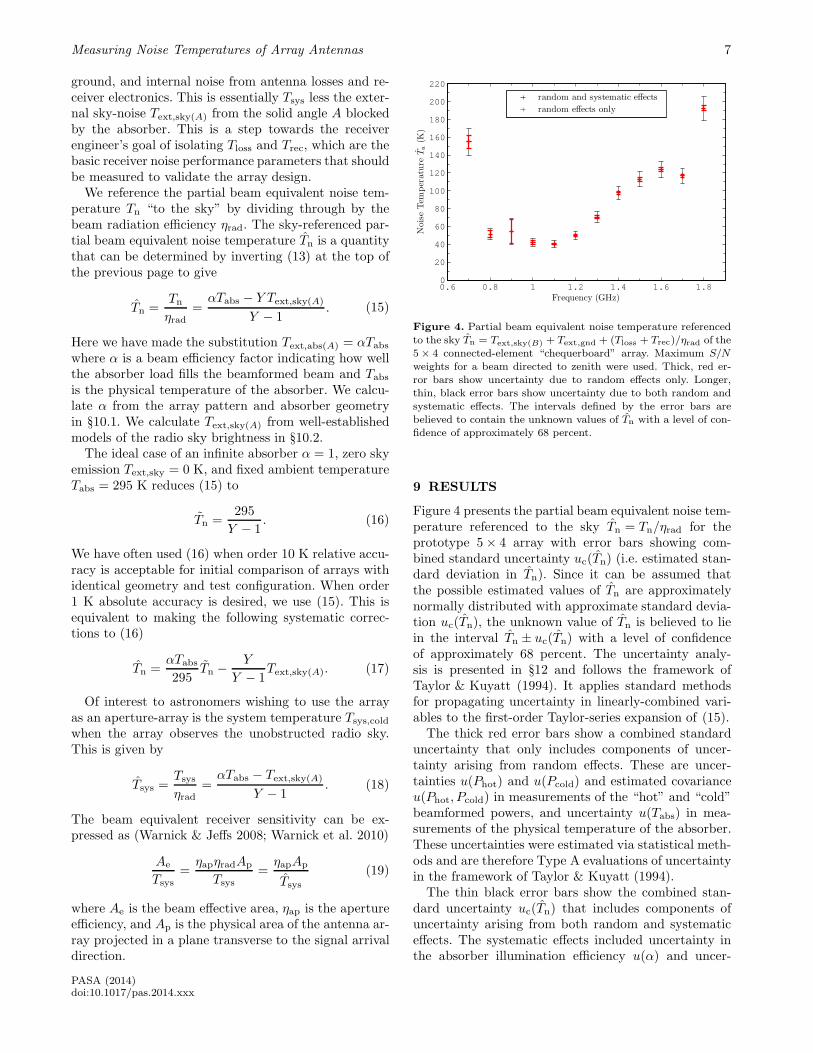
Figure 4. Partial beam equivalent noise temperature referencedto the sky Tn = Text,sky(B) + Text,gnd + (Tloss + Trec)/ηrad of the5× 4 connected-element “chequerboard” array. Maximum S/Nweights for a beam directed to zenith were used. Thick, red er-ror bars show uncertainty due to random effects only. Longer,thin, black error bars show uncertainty due to both random andsystematic effects. The intervals defined by the error bars arebelieved to contain the unknown values of Tn with a level of con-fidence of approximately 68 percent.
9 RESULTS
Figure 4 presents the partial beam equivalent noise tem-perature referenced to the sky Tn = Tn/ηrad for theprototype 5× 4 array with error bars showing com-bined standard uncertainty uc(Tn) (i.e. estimated stan-dard deviation in Tn). Since it can be assumed thatthe possible estimated values of Tn are approximatelynormally distributed with approximate standard devia-tion uc(Tn), the unknown value of Tn is believed to liein the interval Tn ± uc(Tn) with a level of confidenceof approximately 68 percent. The uncertainty analy-sis is presented in §12 and follows the framework ofTaylor & Kuyatt (1994). It applies standard methodsfor propagating uncertainty in linearly-combined vari-ables to the first-order Taylor-series expansion of (15).The thick red error bars show a combined standard
uncertainty that only includes components of uncer-tainty arising from random effects. These are uncer-tainties u(Phot) and u(Pcold) and estimated covarianceu(Phot, Pcold) in measurements of the “hot” and “cold”beamformed powers, and uncertainty u(Tabs) in mea-surements of the physical temperature of the absorber.These uncertainties were estimated via statistical meth-ods and are therefore Type A evaluations of uncertaintyin the framework of Taylor & Kuyatt (1994).The thin black error bars show the combined stan-
dard uncertainty uc(Tn) that includes components ofuncertainty arising from both random and systematiceffects. The systematic effects included uncertainty inthe absorber illumination efficiency u(α) and uncer-
PASA (2014)doi:10.1017/pas.2014.xxx

8 A. P. Chippendale, D. B. Hayman and S. G. Hay
0.6 0.8 1 1.2 1.4 1.6 1.80
20
40
60
80
100
120
140
160
180
200
220
Frequency (GHz)
System
NoiseTem
perature
Tsys(K
)
Galactic CentreOut of Galactic Plane
Figure 5. Beam equivalent system noise temperatureTsys = Text,sky(A) + Text,sky(B) + Text,gnd + (Tloss + Trec)/ηradof the 5× 4 connected-element “chequerboard” array referencedto the sky. Maximum S/N weights for a beam directed to zenithwere used. The data with error bars show the system noisetemperature for the measurement configuration of this paperwhere the array observed the galactic centre. The intervalsdefined by the error bars are believed to contain the unknownvalues of Tsys with a level of confidence of approximately 68percent. The circles without error bars show an estimate ofthe system noise temperature for the array observing out ofthe galactic plane towards the coldest region of radio sky thattransits at the zenith at Parkes (at 3:51 LST). For clarity ofpresentation, error bars are not plotted for this second seriesalthough they will be very close to a scaled copy of the errorbars for the measurement towards the galactic centre.
tainty in the beam equivalent external noise tempera-ture due to the radio sky u(Text,sky(A)) over solid angleA that is blocked by the absorber. Both of these uncer-tainties are functions of the beamformed antenna pat-tern. They are evaluated via assessments of the rangeof plausible beam patterns defined by the uniform andoptimised weights discussed in §10. These assessmentsare Type B (non-statistical) evaluations of uncertaintyaccording to Taylor & Kuyatt (1994).The dominant component of uncertainty was the sys-
tematic effect characterised by u(α). This arises fromthe fact that the beamformed antenna pattern is notmeasured and so is estimated from theory. Uncertaintydue to random effects was dominated at most frequen-cies by the contribution of u(Pcold). At most frequenciesu(Pcold) characterised noise in measured beamformedpower associated with the beam equivalent system tem-perature. This could be reduced by increasing measure-ment bandwidths and/or integration times. However,external RFI was the dominant effect contributing tou(Pcold) and therefore uncertainty due to random ef-fects at 0.9 GHz.For the results in Figure 4 we estimated Text,sky(A)
using weights with uniform amplitudes and phases that
are conjugate matched to the expected spherical wavefrom the reference radiator. These same weights areused in §10.1 to estimate the lower plausible limit ofα. Under the approximate assumption of a directionindependent sky brightness, Text,sky(A) will be directlyproportional to α. Therefore we expect that the uni-form amplitude weights should yield an approximatelower bound for Text,sky(A). This should result in a con-
servative overestimate of Tn via (15).Figure 5 shows the beam equivalent system noise tem-
perature referenced to the sky Tsys = Tsys/ηrad. Thisis a key factor that determines the receiver sensitivityfor an observation towards a particular part of the skyvia (19). It is a property of both the receiver and thereceiver’s orientation with respect to the sky and sur-rounding environment. This is in contrast to Tn whichis controlled to be as close as practical to a property ofthe receiver in isolation.The error bars in Figure 5 show combined standard
uncertainty uc(Tsys). A second trace (blue circles) shows
the expected reduction in Tsys if one of the coldest re-gions of the sky were used for the “cold” scene insteadof the hotter galactic centre that was used in this work.The value of Tn, on the other hand, is significantly lessdependent on the region of sky used as a reference. Al-though it becomes clear in §12 that using a cold regionof sky would reduce uncertainty in Tn.
10 SYSTEMATIC CORRECTIONS
10.1 Absorber Illumination Efficiency
We define the absorber illumination efficiency α as a di-mensionless metric of the beamformed antenna patternD(θ, φ) according to
α =
∫
AD(θ, φ)dΩ
∫
4πD(θ, φ)dΩ
. (20)
This follows the beam efficiency definition of Nash(1964) but with the numerator evaluated over the solidangle subtended by the absorber load A instead of thesolid angle of the main beam. This is equivalent to eval-uating the solid-beam efficiency, defined in the IEEEStandard Definitions of Terms for Antennas (IEEE Std145-1993), for solid angle A but ignoring antenna losses.Figure 6 shows values of α calculated for array pat-
terns formed by two different weightings of 40 isotropicelements arranged with the same geometry as the 5× 4prototype. The weight phases were conjugate matchedto a supposed spherical wavefront emanating from thereference antenna used to constrain beam pointing.Weight amplitudes were assigned according to two dif-ferent methods: uniform amplitudes and an optimisedamplitude taper. These choices are thought to encom-pass the plausible range of amplitude tapers imposedby the maximum S/N weights of (3) with direction and
PASA (2014)doi:10.1017/pas.2014.xxx

Measuring Noise Temperatures of Array Antennas 9
0.6 0.8 1 1.2 1.4 1.6 1.80.8
0.82
0.84
0.86
0.88
0.9
0.92
0.94
0.96
0.98
1
Frequency (GHz)
Absorber
IlluminationEfficien
cyα
uniformoptimum
Figure 6. Absorber beam illumination efficiency α for uniformamplitude weights and weights with amplitude taper optimisedto maximise α. Both sets of weights are conjugate phase matchedto the expected spherical wavefront from the reference radiator.
polarisation constrained by the reference antenna mea-surement.We explored a third amplitude taper function
matched to the expected illumination from the LPDAreference antenna according to pattern measurementsprovided by its manufacturer. The LPDA α result wasnot plotted as it was within 1% of that obtained by theuniform amplitude weights.Based on the range of α exhibited in Figure 6 we as-
sessed that the value of α was highly likely (near 100%probability) to lie in the range α = 0.9± 0.1. Uncer-tainty in α was modelled by a uniform distribution overthis range. We divided the half-range of this distribu-tion of 0.1 by
√3, according to Taylor & Kuyatt (1994),
to estimate the standard uncertainty in the absorber il-lumination efficiency u(α) = 0.0577.The uniform-weight pattern is easy to calculate and
we expect it to give the narrowest main beam but withhigh side lobes. This should perform well at lower fre-quencies where the 5× 4 array is too small to form amain beam that falls entirely within the area blocked bythe absorber load. In fact, the uniform-weight α turnedout to be consistent with the optimised-taper α below1 GHz.The optimised taper was calculated by parameteris-
ing an amplitude taper for an ideal boresight beam withthe following taper function that is separable on x andy coordinates (Nash 1964)
|w| =[
Kx + (1−Kx)(1 − (2x/Lx)2)nx
]
×[
Ky + (1−Ky)(1− (2y/Ly)2)ny
]
.(21)
Here Lx is the linear size of the array along the x-axis.ParametersKx and nx determine the shape of the taperfunction factor that separates along the x-axis.
We tried two constrained optimisation techniques tofind the parameters of (21) that lead to an array patternthat maximised α as calculated by (20), subject to theconstraints 0.1 < K < 0.999 and 0.5 < n < 4. Both theSNOPT implementation (Gill 2013; Gill et al. 2005) ofsequential quadratic programming (SQP) optimisationand Standard Particle Swarm Optimisation SPSO-2011(Clerc 2012; Zambrano-Bigiarini et al. 2013) yielded thesame optimal value of α to within 0.04%.We calculated the array pattern assuming isotropic
elements (array factor) as we wanted a measurementand analysis method that does not require specialknowledge of the array design beyond its geometry. Thisallows measurement and comparison of arrays providedas complete “black-box” systems. Our technique will be-come even more accurate for larger arrays, such as theASKAP 188-port PAFs, that can form narrower beamswith lower side lobes and therefore more efficiently illu-minate the load.A better estimate of the partial beam equivalent noise
temperature may be formed by including simulated ormeasured element patterns, but this is beyond the scopeof the current work. Our technique is fair for the cur-rent array which has element patterns with relativelylow gain. Alternatively, we could force α closer to unityby employing a ground shield to reflect as much of thearray pattern as possible onto the load, by reducing thevertical spacing between the load and the array undertest, or by using a larger load. We are building a groundshield and a larger load for future experiments.
10.2 Sky Brightness
Calculating Tn via (15) or Tsys via (18) requires an es-timate of Text,sky(A). This is the component of pre-lossbeam equivalent noise temperature due to radio emis-sion from the region of sky A blocked by the absorberwhen in position for the “hot” measurement. Figure 7shows a break-down of contributions to Text,sky(A) formeasurements made from the Parkes Test Facility to-wards both the hottest and coolest regions of the radiosky observed during zenith pointing drift scans. Thesehave been calculated with the same uniform amplitudeweights used to estimate α in §10.1.We estimated Text,sky(A) by convolving the sky bright-
ness Tbsky(θ, φ) with the beamformed antenna patternD(θ, φ) to give
Text,sky(A) =
∫
ATbsky(θ, φ)D(θ, φ)dΩ∫
4π D(θ, φ)dΩ. (22)
The numerator is evaluated over the solid angle A sub-tended by the absorber load when in position over thearray under test as shown in Figure 1. The denominatornormalises by the beam solid angle.
PASA (2014)doi:10.1017/pas.2014.xxx

10 A. P. Chippendale, D. B. Hayman and S. G. Hay
0.7 0.8 0.9 1 1.1 1.2 1.3 1.4 1.5 1.6 1.70
5
10
15
20
25
Frequency (GHz)
NoiseTem
perature
(K)
Text,sky(A) (galactic centre)Text,sky(A) (out of galactic plane)GSM (galactic centre)GSM (out of galactic plane)CMBAtmosphereSun
Figure 7. Breakdown of contributions to Text,sky(A), which is thebeam equivalent external noise temperature due to radio emissionfrom the area of sky blocked by the absorber load. The Global SkyModel (GSM) contribution is calculated at 17:39 LST, near tran-sit of the galactic centre, when the measurements for this paperwere made. It is also calculated at 03:51 LST when zenith obser-vations from latitudes near 30S point out of the galactic planetowards one of the coldest patches of radio sky as deduced bymeasured and modelled drift-scans in §7 of Chippendale (2009).The thick lines show total Text,sky(A) for these two limiting ob-servation epochs. The thin lines show the breakdown of thesetotals into contributions from the GSM, cosmic microwave back-ground (CMB), atmosphere, and Sun. The curves for the diffuse
backgrounds (i.e. all but the Sun curve) would be directly pro-portional to α if the sky brightness were direction independent.
The sky brightness is modelled as background radiosky brightness Tb0, attenuated by a dry atmospherewith: air mass X(θ) as a function of zenith angle θ,transmissivity e−τX(θ), and atmospheric noise emissionrepresented by an equivalent physical temperature Tatm
Tbsky(θ, φ) = Tb0(θ, φ)e−τX(θ)
+(1− e−τX(θ))Tatm.(23)
Background sky brightness Tb0 was estimated ateach measurement frequency using the global radio skymodel (GSM) of de Oliveira-Costa et al. (2008) plus anisotropic Cosmological Microwave Background (CMB)contribution of 2.725 K (Fixsen 2009). The integralin (22) was evaluated with 0.5 resolution in θ andφ, which exceeds the 1 resolution of the GSM eval-uated at the frequencies of interest with principal com-ponent amplitudes locked to the the 408 MHz map ofHaslam et al. (1982).The Sun’s contribution is considered by adding
a single pixel to Tb0(θ, φ) with brightness tempera-ture T⊙Ω⊙/Ωpixel. Here T⊙ is the sum of the steadystate component of solar emission plus the mean ofthe slowly changing component, all normalised to themean visible solid angle of the Sun Ω⊙ = 0.22 deg2.
Table 1 Intensity of Solar Radio Emission(Kuz’min & Salomonovich 1966).
Frequency Mean Brightness Temperaturea
f (GHz) T⊙ (K)
0.6 6×10⁵
3×10⁵
b
1.2 2×10⁵
1×10⁵
3.0 8×10⁴
4×10⁴
a The mean brightness temperature is referenced to the mean vis-ible solid angle of the Sun Ω⊙ = 0.22 deg2. This table gives theconstant component and the mean value of the slowly varyingcomponent.b The numerator corresponds to a period of maximum solar ac-tivity and the denominator corresponds to a period of minimumsolar activity.
The spectrum of T⊙ was interpolated by fitting apower law to the single-frequency values tabulated byKuz’min & Salomonovich (1966) and reproduced herein Table 1 for convenience.Dry atmosphere transmissivity e−τ at zenith was cal-
culated according to Annex 2 of ITU RecommendationITU-R P.676-9; typical equivalent physical temperatureof the atmosphere Tatm = 275 K was taken from ITU-R P.372-10; and the air mass versus zenith angle X(θ)model fit of Young (1994) was used.
11 STRAY EXTERNAL NOISE
The “stray” beam equivalent external noise can be bro-ken into sky and ground components. The stray-skynoise Text,sky(B) may be estimated via the same methodas Text,sky(A) in (22), but evaluating the integral in thenumerator over the area of sky not blocked by theabsorber which we label solid angle B. We assumedText,sky(B) was unchanged between “hot” and “cold”measurements, and therefore neglected scattering fromthe sparse metal frame that supports the absorber.Figure 8 shows the resulting Text,sky(B) estimate for
the experiment presented in this paper. It will be high-est when the galactic centre is almost but not quiteblocked by the absorber. It will be lowest when thegalactic centre is near/below the horizon or completelyblocked by the absorber.The stray-ground radiation Text,gnd can also be esti-
mated via (22), but evaluating the integral in the nu-merator over the backward hemisphere and substitut-ing the sky-brightness model with a ground-brightnessmodel Tg(θ, φ). An order of magnitude estimate ofText,gnd may be made by assuming that the groundbrightness takes on the direction independent value ofTg. We would then estimate Text,gnd = (1− ef)Tg. Hereef is the forward efficiency of the beamformed antennapattern. This may be calculated via (20), but with thenumerator evaluated over the full forward hemisphereinstead of just the solid angle blocked by the absorber.
PASA (2014)doi:10.1017/pas.2014.xxx

Measuring Noise Temperatures of Array Antennas 11
0.7 0.8 0.9 1 1.1 1.2 1.3 1.4 1.5 1.6 1.70
0.5
1
1.5
2
2.5
Frequency (GHz)
Stray-SkyNoiseText,sky(B
)(K
)
Figure 8. Antenna temperature component due to stray-sky ra-diation calculated via (22), but evaluating the integral in the nu-merator over the area of sky B not blocked by the absorber. Thiswould be directly proportional to (1 − α) if the sky brightnesswere direction independent.
Stray radiation could be measured by making beam-formed Y-factor measurements with and without aground-shield. As mentioned above, such a groundshield is being manufactured for ongoing noise measure-ments of array receivers at the Parkes Test Facility.
12 MEASUREMENT UNCERTAINTY
Uncertainty in the measured noise temperature was es-timated via the framework of Taylor & Kuyatt (1994).The combined standard error uc(Tn) is an estimate ofthe standard deviation in Tn. This estimate is made viathe linear combination of uncertainties in the first orderTaylor series expansion of (15). This gives
u2c(Tn) =
(
∂Tn
∂Phot
)2
u2(Phot)
+
(
∂Tn
∂Pcold
)2
u2(Pcold)
+ 2
∣
∣
∣
∣
∣
∂Tn
∂Phot
∂Tn
∂Pcold
∣
∣
∣
∣
∣
u (Phot, Pcold)
+
(
∂Tn
∂α
)2
u2(α) +
(
∂Tn
∂Tabs
)2
u2(Tabs)
+
(
∂Tn
∂Text,sky(A)
)2
u2(Text,sky(A))
(24)
where u(x) is an estimate of the standard deviation as-sociated with input estimate x and u(x, y) is an estimateof the covariance associated with input estimates x and
y. Evaluation of the partial derivatives of (15) and sub-stitution of (8) and (18) yields the square of the relativecombined standard uncertainty as a function of inputestimates(
uc(Tn)
Tn
)2
=
(
Tsys
Tn
)2 [(
u(Phot)
Phot
)2
+
(
u(Pcold)
Pcold
)2
+2u (Phot, Pcold)
PhotPcold
]
+
(
αTabs
Y Tn
)2[
(
u(α)
α
)2
+
(
u(Tabs)
Tabs
)2]
+
(
Text,sky(A)
Tn
)2(u(Text,sky(A))
Text,sky(A)
)2
(
Y
Y − 1
)2
.
(25)
Applying the same uncertainty analysis to Tsys as de-fined by (18) yields
(
uc(Tsys)
Tsys
)2
=
[
(
u(Phot)
Phot
)2
+
(
u(Pcold)
Pcold
)2
+2u (Phot, Pcold)
PhotPcold
]
+
(
αTabs
Y Tsys
)2 [(
u(α)
α
)2
+
(
u(Tabs)
Tabs
)2]
+
(
Text,sky(A)
Y Tsys
)2(
u(Text,sky(A))
Text,sky(A)
)2
(
Y
Y − 1
)2
.
(26)
In both (25) and (26), the first term’s dependence onu(Phot) and u(Pcold) suggests that beamformed powermeasurements should be made with adequate integra-tion time and/or measurement bandwidth to reducemeasurement variance via averaging. The first term’sdependence on u(Phot, Pcold) highlights the necessityto minimise gain and/or noise performance drift be-tween “hot” and “cold” measurements. The second termhighlights the importance of knowing the absorber-illumination efficiency α and accurately measuring theambient temperature of the absorber. Good knowledgeof the beam pattern of the array under test is requiredto accurately estimate α. The third term highlightsthe importance of estimating the beamformed antennatemperature which is a function of the backgroundsky brightness and the beamformed antenna pattern.Comparing (25) and (26) shows that u(Text,sky(A)) con-
tributes less uncertainty to Tsys than to Tn, particularlyfor low-noise arrays under test with high Y-factors.Figure 9 shows the contribution of each input uncer-
tainty, via (25), to the combined standard uncertaintyuc(Tn) in partial beam equivalent noise temperature.This shows that the combined uncertainty is largely
PASA (2014)doi:10.1017/pas.2014.xxx

12 A. P. Chippendale, D. B. Hayman and S. G. Hay
0.7 0.8 0.9 1 1.1 1.2 1.3 1.4 1.5 1.6 1.70
2
4
6
8
10
12
14
Frequency (GHz)
Contributionto
uc(Tn)(K
)
u(α)
u(Pcold)
u(Text,sky(A))
u(Phot, Pcold)
u(Phot)
u(Tabs)
Figure 9. Breakdown of contributions to combined uncertaintyuc(Tn) in partial beam equivalent noise noise temperature due toeach input uncertainty in (25).
dominated by uncertainty u(α) in the illumination ofthe absorber, which is in turn due to uncertainty in thebeamformed antenna pattern.In the above uncertainty analysis we have not in-
cluded the correlation between α and Text,sky(A). Thiscorrelation arises as they are both direct functions of thebeamformed antenna pattern. In the future, we couldtake advantage of the fact that the stray external noiseText,sky(B) is also a function of the antenna pattern andcorrelated with α and Text,sky(A). Including these corre-lations in the uncertainty analysis at the same time assubtracting an estimate of Text,sky(B) from Tn may leadto some cancellation in uncertainty terms that dependon the antenna pattern. This could reduce uncertaintyat the same time as moving us closer to extracting Tloss
and Trec from Tn.
13 CONCLUSION
We have demonstrated the measurement of partialbeam equivalent noise temperature as low as Tn = 40 Kwith a combined standard uncertainty (estimated stan-dard deviation) as low as uc(Tn) = 4 K. This combineduncertainty was dominated by uncertainty u(α) in theefficiency with which the beamformed array pattern il-luminates the absorber.The prioritised action-list for reducing uncertainty
further is:
1. Reducing uncertainty in absorber-illumination ef-ficiency α by:
– increasing the solid angle subtended by the ab-sorber by increasing its size or moving it closerto the array under test,
– adding a ground shield to reflect more of theantenna pattern onto the absorber, or
– accurately measuring or modelling the beam-formed antenna pattern.
2. Moving the reference radiator into the far field ofthe array under test.
3. Increasing integration time for the “cold” sky mea-surement.
4. Reducing uncertainty in beam equivalent noisetemperature due to radio emission from the skyText,sky(A) by:
– using the coldest possible region of the sky forthe “cold” sky measurement,
– accurately measuring or modelling the beam-formed antenna pattern, and
– improving the accuracy of the global sky model.
Addressing items (1) to (3) would reduce the mediancombined standard uncertainty to just uc(Tn) = 2 Kover 0.7 GHz to 1.8 GHz.
14 ONGOING DEVELOPMENT
After the measurements were made for this paper, theParkes test facility was upgraded to include a 192-portdown-conversion and digital receiver system. This sup-ports 304 MHz instantaneous bandwidth tunable over0.7 GHz to 1.8 GHz with 1 MHz spectral resolution. Itis capable of online measurement of the full 192× 192correlation matrix and online beamforming for nine si-multaneous dual-polarisation beams.This was achieved by installing the electronics that
are normally found in the pedestal of ASKAP’s first six“BETA” antennas (Schinckel et al. 2011; Bunton et al.2011) into a hut near the test-pad. This receiver canbe connected to test arrays mounted on the aperture-array test pad or at the focus of the nearby 12 m dishvia RF coaxial cables in trenches. The upgraded facil-ity was recently used to verify an enhanced ASKAPLNA and chequerboard array design that has low-noise performance over the full 0.7 GHz to 1.8 GHzband (Shaw et al. 2012). This improvement will be in-cluded in the ASKAP Design Enhancements (ADE)PAF (Hampson et al. 2012). The facility was also usedto characterise the astronomical performance of a 188-port BETA PAF that is currently installed at the focusof the 12 m dish.In the future, better estimates of the array noise
properties may be obtained by electromagnetic mod-elling of test setups and the external environmentalcontribution with or without a shield. Work is un-derway to build a ground shield to both reduce u(α)and allow estimation of “stray” beam equivalent exter-nal noise Text,sky(B) + Text,gnd. We are also building alarger absorber load for use at our radio quiet site at the
PASA (2014)doi:10.1017/pas.2014.xxx

Measuring Noise Temperatures of Array Antennas 13
Murchison Radioastronomy Observatory (MRO) whereASKAP is sited. This radio quiet site will allow morerepeatable noise measurements below 1 GHz where theRFI situation at Parkes becomes challenging.
15 ACKNOWLEDGEMENTS
The Australian SKA Pathfinder is part of the AustraliaTelescope National Facility which is funded by the Com-monwealth of Australia for operation as a National Facilitymanaged by CSIRO. The “chequerboard” array and systemdevelopment has been the work of the ASKAP team.
The LNAs and downconversion modules for the prototypepresented in this paper were designed by Alex Grancea. JohnBunton developed the digital system architecture whichwas implemented by Joseph Pathikulangara, Jayasri Joseph,Tim Bateman, Andrew Brown and Dezso Kiraly. Malte Mar-quarding, Juan Carlos Guzman, Euan Troup, David Bro-drick and Simon Hoyle developed and supported software tooperate the system. Tim Wilson did the mechanical designfor the structure supporting the absorber load. The staff atthe CSIRO Parkes Observatory, including Brett Preisig, IanMcRobert, Tom Lees and Jon Crocker have supported thetesting by developing the infrastructure, including the ab-sorber load, and responding rapidly to diverse needs duringmeasurement campaigns.
The array measurements at Parkes, leading up to andincluding the measurements presented in this paper, wereconducted by Robert Shaw, Ian McRobert, Tim Bateman,Peter Axtens, Russell Gough, John O’Sullivan and KjetilWormnes in addition to the authors. Preparation work inSydney has been supported by many colleagues, includingCarl Holmesby, Ivan Kekic and Ken Smart. Russell Gough,Aidan Hotan and John Bunton also provided helpful com-ments on intermediate drafts.
REFERENCES
Alexander, P., Bolton, R., Faulkner, A., Torchinsky,S., van Ardenne, A., Wilkinson, P., de Vos, M.,Bakker, L., Garrington, S., Harris, G., Ikin, T.,Jones, M., Kant, D., McCool, R., & Patel, P. 2007,SKADS Benchmark Scenario Design and Costing,SKA Memo 93
Bunton, J., Hampson, G., Brown, A., Pathikulangara,J., Tuthill, J., Souza, L., Joseph, J., Bateman, T., &Neuhold, S. 2011, in General Assembly and ScientificSymposium, 2011 XXXth URSI, 1–4
Chippendale, A., O’Sullivan, J., Reynolds, J., Gough,R., Hayman, D., & Hay, S. 2010, in 2010 IEEE Inter-national Symposium on Phased Array Systems andTechnology (ARRAY), 648–652
Chippendale, A. P. 2009, Phd, The University of Sydney
Chippendale, A. P., Colegate, T. M., & O’Sullivan, J. D.2007, SKAcost: a Tool for SKA Cost and PerformanceEstimation, SKA Memo 92
Clerc, M. 2012, Standard Particle SwarmOptimisation, Tech. rep., 15 pages,
http://hal.archives-ouvertes.fr/hal-00764996
Compton, Jr., R. T. 1988, Adaptive Antennas: Con-cepts and Performance (Prentice Hall)
de Oliveira-Costa, A., Tegmark, M., Gaensler, B. M.,Jonas, J., Landecker, T. L., & Reich, P. 2008, MN-RAS, 388, 247
DeBoer, D. R., Gough, R. G., Bunton, J. D., Corn-well, T. J., Beresford, R. J., Johnston, S., Feain, I. J.,Schinckel, A. E., Jackson, C. A., Kesteven, M. J.,Chippendale, A., Hampson, G. A., O’Sullivan, J. D.,Hay, S. G., Jacka, C. E., Sweetnam, T. W., Storey,M. C., Ball, L., & Boyle, B. J. 2009, Proc. IEEE, 97,1507
Dewdney, P., Hall, P., Schilizzi, R., & Lazio, T. 2009,Proc. IEEE, 97, 1482
Dewdney, P. E. 2013, SKA1 System Baseline Design,Tech. Rep. SKA-TEL-SKO-DD-001, SKA Organisa-tion, Manchester
Fixsen, D. J. 2009, ApJ, 707, 916
Fridman, P. A. 2001, A&A, 368, 369
Gill, P., Murray, W., & Saunders, M. 2005, SIAM Re-view, 47, 99
Gill, P. E. 2013, SNOPT (Stu-dent Version) [Computer Software],http://www.scicomp.ucsd.edu/~peg/Software.html
Hampson, G., Macleod, A., Beresford, R., Brothers, M.,Brown, A., Bunton, J., Cantrall, C., Chekkala, R.,Cheng, W., Forsyth, R., Gough, R., Hay, S., Kana-pathippillai, J., Kiraly, D., Leach, M., Morison, N.,Neuhold, S., Roberts, P., Shaw, R., Schinckel, A.,Shields, M., & Tuthill, J. 2012, in Electromagnetics inAdvanced Applications (ICEAA), 2012 InternationalConference on, 807–809
Haslam, C. G. T., Salter, C. J., Stoffel, H., & Wilson,W. E. 1982, A&AS, 47, 1
Hay, S. 2010a, in 2010 International Conference on Elec-tromagnetics in Advanced Applications (ICEAA),649–652
Hay, S., O’Sullivan, J., Kot, J., Granet, C., Grancea, A.,Forsyth, A. R., & Hayman, D. 2007, in Antennas andPropagation, 2007. EuCAP 2007. The Second Euro-pean Conference on, 1–5
Hay, S., O’Sullivan, J., & Mittra, R. 2011, IEEE Trans.Antennas Propag., 59, 1828
Hay, S. G. 2010b, IJMOT, 5, 375
Hay, S. G. & O’Sullivan, J. D. 2008, Radio Science, 43
Hayman, D., Bird, T., Esselle, K., & Hall, P. 2010, IEEETrans. Antennas Propag., 58, 1922
Hayman, D. B., Beresford, R., Bunton, J. D., Cantrall,C., Cornwell, T., Grancea, A., Granet, C., Joseph,J., Kesteven, M. J., O’Sullivan, J. D., Pathikulan-gara, J., Sweetnam, A. W., & Voronkov, M. 2008, inProceedings of the Workshop on the Applications ofRadio Science, Broadbeach, QLD
PASA (2014)doi:10.1017/pas.2014.xxx

14 A. P. Chippendale, D. B. Hayman and S. G. Hay
Kuz’min, A. D. & Salomonovich, A. E. 1966, Radioas-tronomical Methods of Antenna Measurements (NewYork: Academic Press)
Lo, Y., Lee, S.-W., & Lee, Q. H. 1966, Proc. IEEE, 54,1033
Monzingo, R. A., L., H. R., & W., M. T. 2011, Intro-duction to Adaptive Arrays, 2nd edn. (Raleigh, NC:SciTech)
Nash, R. T. 1964, IEEE Trans. Mil. Electron., 8, 252
Nita, G. M. & Gary, D. E. 2010, MNRAS, 406, L60
Nita, G. M., Gary, D. E., Liu, Z., Hurford, G. J., &White, S. M. 2007, PASP, 119, 805
Reed, I., Mallett, J., & Brennan, L. 1974, IEEE Trans.Aerosp. Electron. Syst., AES-10, 853
Schilizzi, R. T., Alexander, P., Cordes, J. M., Dewdney,P. E., Ekers, R. D., Faulkner, A. J., Gaensler, B. M.,Hall, P. J., Jonas, J. L., & Kellermann, K. I. 2007,Preliminary Specifications for the Square KilometreArray, SKA Memo 100
Schinckel, A., Bunton, J., Chippendale, A., Gough, R.,Hampson, G., Hay, S., Jackson, C., Jeganathan, K.,O’Sullivan, J., Reynolds, J., Shaw, R., & Wilson, C.2011, in Microwave Conference Proceedings (APMC),2011 Asia-Pacific, 1178–1181
Shaw, R., Hay, S., & Ranga, Y. 2012, in Electromag-netics in Advanced Applications (ICEAA), 2012 In-ternational Conference on, 438–441
Sinclair, M. W. & Gough, R. G. 1991, in IREECON’91
Taylor, B. N. & Kuyatt, C. E. 1994, Guidelines for Eval-uating and Expressing the Uncertainty of NIST Mea-surement Results, NIST Technical Note 1297
Warnick, K. F. 2009, in Antenna Technology (iWAT2009), IEEE International Workshop on
Warnick, K. F., Ivashina, M., Maaskant, R., & Woesten-burg, B. 2010, IEEE Trans. Antennas Propag., 58,2121
Warnick, K. F. & Jeffs, B. 2008, IEEE Antennas Wire-less Propag. Lett., 7, 565
Widrow, B., Mantey, P., Griffiths, L., & Goode, B. B.1967, Proc. IEEE, 55, 2143
Wilson, W. E., Ferris, R. H., Axtens, P., Brown, A.,Davis, E., Hampson, G., Leach, M., Roberts, P.,Saunders, S., Koribalski, B. S., Caswell, J. L., Lenc,E., Stevens, J., Voronkov, M. A., Wieringa, M. H.,Brooks, K., Edwards, P. G., Ekers, R. D., Emonts,B., Hindson, L., Johnston, S., Maddison, S. T., Ma-hony, E. K., Malu, S. S., Massardi, M., Mao, M. Y.,McConnell, D., Norris, R. P., Schnitzeler, D., Sub-rahmanyan, R., Urquhart, J. S., Thompson, M. A.,& Wark, R. M. 2011, MNRAS, 416, 832
Woestenburg, E. E. M., Bakker, L., & Ivashina, M.2012, IEEE Trans. Antennas Propag., 60, 915
Woestenburg, E. E. M., Bakker, L., Ruiter, M.,Ivashina, M., & Witvers, R. 2011, in Microwave Con-
ference (EuMC), 2011 41st European, 1277–1280
Woestenburg, E. E. M. & Dijkstra, K. F. 2003, in Mi-crowave Conference, 2003. 33rd European, 363–366
Young, A. T. 1994, Applied Optics, 33, 1108
Zambrano-Bigiarini, M., Clerc, M., & Rojas, R. 2013,in Evolutionary Computation (CEC), 2013 IEEECongress on, 2337–2344
PASA (2014)doi:10.1017/pas.2014.xxx