Embed Size (px)
Citation preview
^Åèìáëáíáçå=oÉëÉ~êÅÜ=mêçÖê~ã=dê~Çì~íÉ=pÅÜççä=çÑ=_ìëáåÉëë=C=mìÄäáÅ=mçäáÅó=k~î~ä=mçëíÖê~Çì~íÉ=pÅÜççä=
SYM-AM-16-062
mêçÅÉÉÇáåÖë=çÑ=íÜÉ=
qÜáêíÉÉåíÜ=^ååì~ä=^Åèìáëáíáçå=oÉëÉ~êÅÜ=
póãéçëáìã=
qÜìêëÇ~ó=pÉëëáçåë=sçäìãÉ=ff= =
A Complex Systems Perspective of Risk Mitigation and Modeling in Development and Acquisition Programs
Roshanak Rose Nilchiani, Associate Professor, Stevens Institute of Technology Antonio Pugliese, PhD Student, Stevens Institute of Technology
Published April 30, 2016
Approved for public release; distribution is unlimited.
Prepared for the Naval Postgraduate School, Monterey, CA 93943.

^Åèìáëáíáçå=oÉëÉ~êÅÜ=mêçÖê~ã=dê~Çì~íÉ=pÅÜççä=çÑ=_ìëáåÉëë=C=mìÄäáÅ=mçäáÅó=k~î~ä=mçëíÖê~Çì~íÉ=pÅÜççä=
The research presented in this report was supported by the Acquisition Research Program of the Graduate School of Business & Public Policy at the Naval Postgraduate School.
To request defense acquisition research, to become a research sponsor, or to print additional copies of reports, please contact any of the staff listed on the Acquisition Research Program website (www.acquisitionresearch.net).
^Åèìáëáíáçå=oÉëÉ~êÅÜ=mêçÖê~ãW=`êÉ~íáåÖ=póåÉêÖó=Ñçê=fåÑçêãÉÇ=`Ü~åÖÉ= - 194 -
Panel 16. Improving Governance of Complex Systems Acquisition
Thursday, May 5, 2016
11:15 a.m. – 12:45 p.m.
Chair: Rear Admiral David Gale, USN, Program Executive Officer, SHIPS
Complex System Governance for Acquisition
Joseph Bradley, President, Leading Change, LLC Polinpapilinho Katina, Postdoctoral Researcher, Old Dominion University Charles Keating, Professor, Old Dominion University
Acquisition Program Teamwork and Performance Seen Anew: Exposing the Interplay of Architecture and Behaviors in Complex Defense Programs
Eric Rebentisch, Research Associate, MIT Bryan Moser, Lecturer, MIT John Dickmann, Vice President, Sonalysts Inc.
A Complex Systems Perspective of Risk Mitigation and Modeling in Development and Acquisition Programs
Roshanak Rose Nilchiani, Associate Professor, Stevens Institute of Technology Antonio Pugliese, PhD Student, Stevens Institute of Technology
^Åèìáëáíáçå=oÉëÉ~êÅÜ=mêçÖê~ãW=`êÉ~íáåÖ=póåÉêÖó=Ñçê=fåÑçêãÉÇ=`Ü~åÖÉ= - 231 -
A Complex Systems Perspective of Risk Mitigation and Modeling in Development and Acquisition Programs
Roshanak R. Nilchiani—is an Associate Professor of Systems Engineering at the Stevens Institute of Technology. She received her BSc in mechanical engineering from Sharif University of Technology, MS in engineering mechanics from University of Nebraska–Lincoln, and PhD in aerospace systems from Massachusetts Institute of Technology. Her research focuses on computational modeling of complexity and system ilities for space systems and other engineering systems, including the relationship between system complexity, uncertainty, emergence, and risk. The other track of her current research focuses on quantifying, measuring, and embedding resilience and sustainability in large-scale critical infrastructure systems. [[email protected]]
Antonio Pugliese—received his BSc and MSc in aerospace engineering from the University of Naples Federico II in Naples, Italy, in 2010 and 2012, respectively. He also received a postgraduate Master in Systems Engineering for Aerospace Applications (SEAMIAero) from the University of Naples Federico II in 2014. He is currently a PhD student in systems engineering at the Stevens Institute of Technology in Hoboken, NJ. He worked on winged atmospheric re-entry systems, focusing on flight quality and thermal protection systems. He also has experience as a systems engineer with attitude control systems and experimental payloads for sounding rockets. [[email protected]]
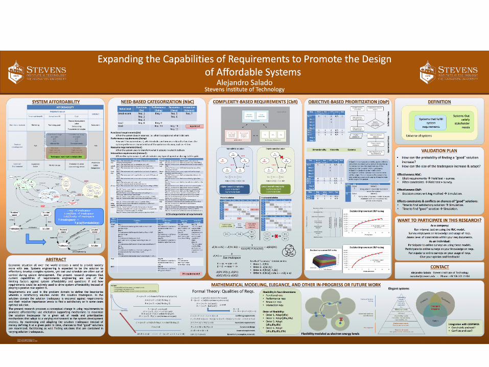
Abstract The current methodologies used in risk assessment are heavily subjective and inaccurate in various life cycle phases of complex engineered systems. The increase in complexity has caused a paradigm shift from root cause analysis to the search of a set of concurrent causes for each event and the relevant complexity content of the system. Many of the system’s life cycle risks are currently assessed subjectively by imprecise methodologies such as color-coded risk matrix, and subsequently they suffer from unforeseen failures as well as cost and schedule overruns. This research project proposes a novel approach to major improvement of risk assessment by creating a set of appropriate complexity measures (informed by historical case studies) as pre-indicators of emergence of risks at different stages of a systems development process, and also a framework that enables the decision-makers on assessing the actual risk level at each phase of the development based on requirements, design decisions, and alternatives. The goal of this research is to capture the complexity of the system with some innovative metrics, thus allowing for better decision-making in architecture and design selections.
Introduction Engineered systems have become progressively more complex and interconnected
to other various infrastructure systems over the past few decades, and they continue to become more complex. Examples of this can be seen in various fields of engineered systems, spanning from satellites, aircrafts, and missiles to ground transportation systems and sophisticated interconnected power and communication grids. In one perspective, more complexity provides more sophisticated multi-functionality to the engineered system at hand, while in a competing perspective, concurrently can make the system more vulnerable and fragile and prone to failures and emergent behavior. The relationship between excessive complexity in design and operation of complex engineered systems to the risk, emergence, and increased manifestation of failures has been acknowledged by many experts and academics in various engineering design communities. However, there is a lack of comprehensive research that enables the discovery of the relationship between the level of complexity of a design to increased risks and failure of that system. This research is an initial study in understanding, modeling, and suggesting relevant complexity measures in
^Åèìáëáíáçå=oÉëÉ~êÅÜ=mêçÖê~ãW=`êÉ~íáåÖ=póåÉêÖó=Ñçê=fåÑçêãÉÇ=`Ü~åÖÉ= - 232 -
engineering design that can be used and linked quantitatively to the risk assessment of an engineered system.
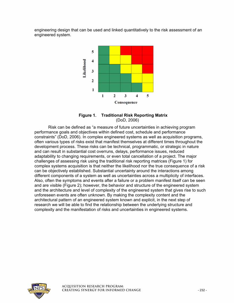
Traditional Risk Reporting Matrix (DoD, 2006)
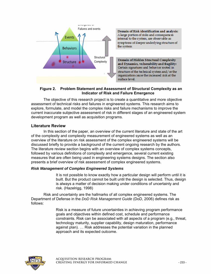
Risk can be defined as “a measure of future uncertainties in achieving program performance goals and objectives within defined cost, schedule and performance constraints” (DoD, 2006). In complex engineered systems as well as acquisition programs, often various types of risks exist that manifest themselves at different times throughout the development process. These risks can be technical, programmatic, or strategic in nature and can result in substantial cost overruns, delays, performance issues, reduced adaptability to changing requirements, or even total cancellation of a project. The major challenges of assessing risk using the traditional risk reporting matrices (Figure 1) for complex systems acquisition is that neither the likelihood nor the true consequence of a risk can be objectively established. Substantial uncertainty around the interactions among different components of a system as well as uncertainties across a multiplicity of interfaces. Also, often the symptoms and events after a failure or a problem manifest itself can be seen and are visible (Figure 2); however, the behavior and structure of the engineered system and the architecture and level of complexity of the engineered system that gives rise to such unforeseen events are often unknown. By making the complexity content and the architectural pattern of an engineered system known and explicit, in the next step of research we will be able to find the relationship between the underlying structure and complexity and the manifestation of risks and uncertainties in engineered systems.
^Åèìáëáíáçå=oÉëÉ~êÅÜ=mêçÖê~ãW=`êÉ~íáåÖ=póåÉêÖó=Ñçê=fåÑçêãÉÇ=`Ü~åÖÉ= - 233 -
Problem Statement and Assessment of Structural Complexity as an Indicator of Risk and Failure Emergence
The objective of this research project is to create a quantitative and more objective assessment of technical risks and failures in engineered systems. This research aims to explore, formulate, and model the complex risks and failure mechanisms to improve the current inaccurate subjective assessment of risk in different stages of an engineered system development program as well as acquisition programs.
Literature Review In this section of the paper, an overview of the current literature and state of the art
of the complexity and complexity measurement of engineered systems as well as an overview of the literature on risk assessment of the complex engineered systems will be discussed briefly to provide a background of the current ongoing research by the authors. The literature review section begins with an overview of complex systems concepts, followed by various definitions of complexity and emergence, several current existing measures that are often being used in engineering systems designs. The section also presents a brief overview of risk assessment of complex engineered systems.
Risk Management of Complex Engineered Systems
It is not possible to know exactly how a particular design will perform until it is built. But the product cannot be built until the design is selected. Thus, design is always a matter of decision making under conditions of uncertainty and risk. (Hazelrigg, 1998)
Risk and uncertainty are the hallmarks of all complex engineered systems. The Department of Defense in the DoD Risk Management Guide (DoD, 2006) defines risk as follows:
Risk is a measure of future uncertainties in achieving program performance goals and objectives within defined cost, schedule and performance constraints. Risk can be associated with all aspects of a program (e.g., threat, technology maturity, supplier capability, design maturation, performance against plan). … Risk addresses the potential variation in the planned approach and its expected outcome.
^Åèìáëáíáçå=oÉëÉ~êÅÜ=mêçÖê~ãW=`êÉ~íáåÖ=póåÉêÖó=Ñçê=fåÑçêãÉÇ=`Ü~åÖÉ= - 234 -
In general, risks have three components, which are the root cause, a probability (or likelihood) assessed at the present time of the root cause occurring, and the consequence (or effect) of occurrence. Often a root cause is the most basic reason for the presence of a risk. Accordingly, risks should be tied to future root causes and their effects (DoD, 2006).
In any complex technical engineering project, risk can be classified as either of technical or programmatic nature, the former concerning performance criteria and the latter focusing on cost and schedule. Both types of risk are often modeled as the product of the probability of an event and its severity (Pennock & Haimes, 2002). In modeling risk, one can also consider the future root cause (yet to happen) of a certain event (Nilchiani et al., 2013), which is where one is supposed to act in order to eliminate a specific risk. Severity and probability are traditionally represented on the widely utilized, color-coded, risk matrix. Figure 1 shows a color-coded risk matrix. Unfortunately, this seemingly quantitative tool hides subjectivity in the estimation of event frequency and severity, and for those reasons is “inapt for today’s complex systems” (Hessami, 1999). This not only means that most of the systems that we build today cannot be built with the tools and processes from last century, but also that we have started building in a domain where structural patterns matter, especially for large projects.
Complex Systems
Complexity has been one of the characteristics of many large-scale engineered systems of the past century. Complex engineered systems can provide sophisticated functionality as one side of the coin, and the other side can cause the system to be more prone to unwanted emergent behaviors and more fragility to the engineered system. The field of complexity is rich and spans over the past half century in various fields of knowledge ranging from biological systems to cyber-physical systems. As it has been discussed by several researchers, a strong correlation can be observed between the complexity of the system and various ranges of failures, including catastrophic failures (Cook, 1998; Bar-Yam, 2003; Merry & Kassavin, 1995).
In 1948, Warren Weaver, a pioneer in classifying and defining complexity in systems, described three distinct types of problems: problems of simplicity, problems of disorganized complexity, and problems of organized complexity (Weaver, 1948).
According to Weaver (1948), problems of simplicity are the problems with a low number of variables that have been tackled in the 19th century. An example is the classical Newtonian mechanics, where the motion of a body can be described with differential equations in three dimensions. In these problems, the behavior of the system is predicted by integrating equations that describe the behavior of its components. In the same article, Weaver discusses that problems of disorganized complexity are the ones with a very large number of variables that have been tackled in the twentieth century. The most immediate example is the motion of gas particles, or as an analogy the motion of a million balls rolling on a billiard table. The statistical methods developed are applicable when particles behave in an unorganized way and their interaction is limited to the time they touch each other, which is very short. In these problems it has been possible to describe the behavior of the system without looking at its components or the interaction among them.
Problems of organized complexity are the ones that are to be tackled in the 21st century, and ones that see many variables showing the feature of organization. These problems have variables that are closely interrelated and influence each other dynamically. This high level of interaction that gives rise to organization is the reason that these problems cannot be solved easily. Weaver described them as solvable with the help of powerful
^Åèìáëáíáçå=oÉëÉ~êÅÜ=mêçÖê~ãW=`êÉ~íáåÖ=póåÉêÖó=Ñçê=fåÑçêãÉÇ=`Ü~åÖÉ= - 235 -
calculators, but today’s technology is not yet able to solve the most complex of these problems. These are the problems that nowadays we define as “complex.”
Predicting the behavior of a system with many interconnected parts changing their behavior according to the state of other components is a problem of organized complexity, and the system itself is a referred to as a complex system.
Cotsaftis (2009) gives a way of determining whether a system is simple, complicated, or complex by looking at its network model (i.e., nodes and edges). The model defines three types of edges: a free flight state vertex , a driven state from outer source vertex , and an interactive state with other system components vertex . The edges are channels along which there is a resource flux , , or . When
≫ , inf ,, (1)
the ith component is weakly coupled with the others, external and internal. The dynamics of the component can in this case be considered independent from the other components. If the majority of the components satisfy inequality (1) the system is considered to be simple. When
≫ , inf , (2)
the ith component is depending on outside sources. The system can still be partitioned in a set of weakly connected subsystems which dynamics is determined from outside sources. If the majority of the components satisfy inequality (2) the system is considered to be complicated. When
inf ≫ , (3)
the ith component is strongly connected to the others, and its dynamics cannot be determined without considering the effects of the other components. Also, the manipulation of the system cannot be performed as in the previous cases, since the internal connections create conditions that reduce the number of degrees of freedom. A system with a reduced number of external control dimensions that satisfies inequality (3) is said to be complex.
This definition is rather qualitative, since not all the nodes in the system have the same importance (in terms of connection number and intensity) and therefore it makes no sense to consider the majority. For this reason Cotsaftis defines the index of complexity as
/ , where is the number of components that satisfy inequality (3) and N is the total number of components. A complicated system has 0. 1 corresponds to the most complex system possible, but it is also a system where external connections are negligible, and therefore the system is isolated. This is due to the fact that a complex system is describable with a low number of parameters if seen from outside, but has high connectivity in its internal structure.
Considering as an example a sheepdog and a herd of cattle, we realize that the dog has only two degrees of freedom while the herd has 2 , where n is the number of animals in the herd. By pushing the cattle together, the dog increases their interactions and decreases the number of degrees of freedom of the herd to only two, therefore being able to control it.
The research from these two authors has shown us how complexity and simplicity are interrelated concepts, somehow opposite, but that can also be found in the same system at the same time, depending on the point of view. Madni made a distinction between systemic elegance, which “thrives on simplicity through minimalistic thinking and parsimony” and perceived elegance, which “hides systemic or organizational complexity from the user.” If the system is considered to be complex but its complexity can be somehow hidden or
^Åèìáëáíáçå=oÉëÉ~êÅÜ=mêçÖê~ãW=`êÉ~íáåÖ=póåÉêÖó=Ñçê=fåÑçêãÉÇ=`Ü~åÖÉ= - 236 -
resolved, thus making it simpler, then the design can be considered elegant (Madni, 2012). Therefore, in order to achieve a more elegant design, we need to decrease the complexity of the system.
Emergence
Emergence is a major phenomenon related to complex engineered systems. Emergence at the macro-level is not hard-coded at the micro-level (Page, 1999). One example of emergence in natural systems is wetness. Water molecules can be arranged in three different phases (i.e., solid, liquid, and gas), but only one of them expresses a particular type of behavior, which is high adherence to surfaces. This behavior is due to the intermolecular hydrogen bonds that affect the surface tension of water drops. These bonds are also active in the solid and liquid phase, but in those cases they are either too strong or too weak to generate wetness. In this case, the emergence of a property, such as wetness, has been explained at a lower level by looking at the molecules that make up the liquid.
According to Kauffmann (2007), two different types of emergence exists (Kauffman, 2007). The reductionist approach sees emergence as epistemological, meaning that the knowledge about the systems is not yet adequate to describe the emergent phenomenon, but it can improve and explain it in the future. This is the case of wetness, where knowledge about molecules and intermolecular interactions has explained the phenomenon. On the other hand, there is the ontological emergence approach, which says that “not only do we not know if that will happen, [but] we don’t even know what can happen,” meaning that there is a gap to fill not only about the outcome of an experiment (or process), but also about the possible outcomes.
Longo presents this view with the example of the swimming bladder in fishes (Longo, Montevil, & Kauffman, 2012). An organ that gives neutral buoyancy in the water column as its main function, also enables the evolution of some kinds of worms and bacteria that will live in it. Ontological (or radical) emergence is given by the enormous amount of states the system could evolve into. In these cases we not only are not able to predict which state will happen, but we do not even know what the possible states are.
Gell-Mann also pointed out this difference using the concept of logical depth (Gell-Mann, 1995). When some apparently complex behavior can be expressed with simpler laws that reside at a lower level (e.g., the complicated pattern of energy levels of atomic nuclei that can be described at the subatomic level), the phenomenon is said to have a substantial amount of logical depth.
In our research, the emergence that is going to be tackled is considered to be epistemological emergence, logical depth according to Gell-Mann, where knowledge about the system organizational patterns and internal structure can lead to the explanation of certain phenomena. Unfortunately this concept is not so common in the systems engineering and risk management fields, and therefore this research adopts the industry jargon by talking about complexity and complex systems, but always reminding that we are actually trying to unravel logical depth from a systems engineering perspective.
Definitions and Measures of Complexity
There are various definition of complexity that have roots in various fields spanning from mathematics and biology to engineering design. In a recent paper, Wade (2014) suggests that existing complexity definitions belong to one of three types: behavioral, structural, or constructive. Behavioral definitions view the system as a black box and the measures of complexity are given based on the outputs of the system. Structural definitions look at the internal structure or architecture of the system. Constructive definitions see
^Åèìáëáíáçå=oÉëÉ~êÅÜ=mêçÖê~ãW=`êÉ~íáåÖ=póåÉêÖó=Ñçê=fåÑçêãÉÇ=`Ü~åÖÉ= - 237 -
complexity as the difficulty in determining the system outputs (Wade & Heydari, 2014). In this research we are interested in the modeling behavioral and structural complexity metrics. A summary of behavioral complexity definition as well as structural complexity and some measures are presented in the following sections of the literature review.
Behavioral Complexity Definitions and Metrics
The most famous behavioral complexity metric is with no doubt Shannon’s entropy (Shannon, 1948). This metric evaluates the complexity by measuring the entropy of the output message of the system (this metric was initially applied to information systems).
Gell-Mann used Shannon’s entropy to define information measure as a metric capable of measuring both the effective complexity, which is the amount of information necessary to describe the identified regularities of an entity, and the total information, which also takes into account the apparently random features (Gell-Mann & Lloyd, 1996). Algorithmic information content and Shannon entropy are used to build this metric. The former is responsible for measuring the effective complexity (knowledge), and the latter the random parts (ignorance). This dual approach is an interesting contribution to the measurement of complexity, since it allows one to group similar entities according to their effective complexity and to measure the diversity of the ensemble as entropy.
Chaisson (2004) proposed a specific energy-based measure of complexity—more precisely, energy rate density, which is “the amount of energy available for work while passing through a system per unit time and per unit mass” (Chaisson, 2015). This metric looks at the system as a black box and measures the net energy amount entering the system. It has been evaluated for multiple entities such as galaxies, stars, planets, plants, animals, societies, and technological systems, and also has been mapped throughout their lifetime showing an increase in complexity (Chaisson, 2014).
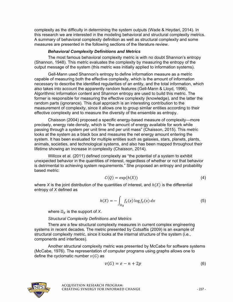
Willcox et al. (2011) defined complexity as “the potential of a system to exhibit unexpected behavior in the quantities of interest, regardless of whether or not that behavior is detrimental to achieving system requirements.” She proposed an entropy and probability based metric:
exp (4)
where X is the joint distribution of the quantities of interest, and is the differential entropy of X defined as
log (5)
where Ω is the support of X.
Structural Complexity Definitions and Metrics
There are a few structural complexity measures in current complex engineering systems in recent decades. The metric presented by Cotsaftis (2009) is an example of structural complexity metric, since it looks at the internal structure of the system (i.e., components and interfaces).
Another structural complexity metric was presented by McCabe for software systems (McCabe, 1976). The representation of computer programs using graphs allows one to define the cyclomatic number as
2 (6)
^Åèìáëáíáçå=oÉëÉ~êÅÜ=mêçÖê~ãW=`êÉ~íáåÖ=póåÉêÖó=Ñçê=fåÑçêãÉÇ=`Ü~åÖÉ= - 238 -
where is the graph, is the number of edges, is the number of nodes, and is the number of connected components. This same metric has been extended to measure architectural design complexity of a system (McCabe & Butler, 1989).
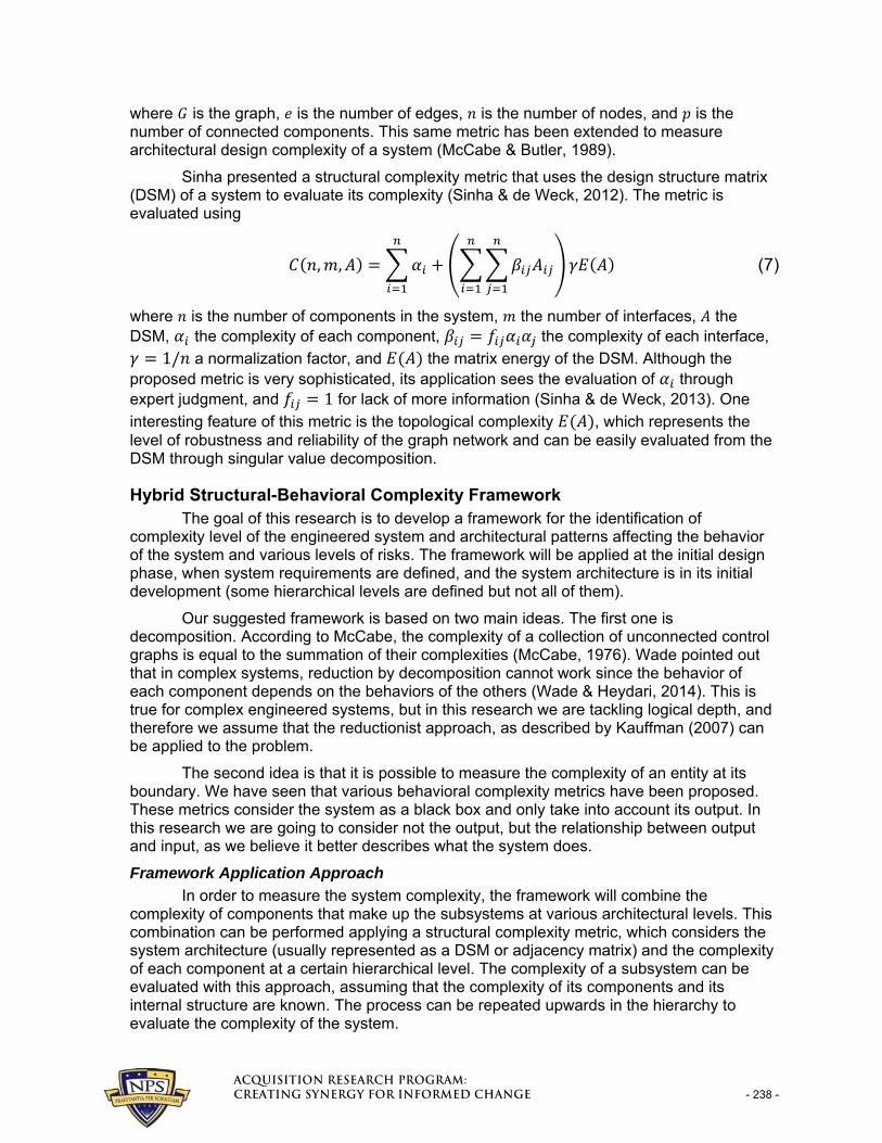
Sinha presented a structural complexity metric that uses the design structure matrix (DSM) of a system to evaluate its complexity (Sinha & de Weck, 2012). The metric is evaluated using
, , (7)
where is the number of components in the system, the number of interfaces, the DSM, the complexity of each component, the complexity of each interface,
1/ a normalization factor, and the matrix energy of the DSM. Although the proposed metric is very sophisticated, its application sees the evaluation of through expert judgment, and 1 for lack of more information (Sinha & de Weck, 2013). One
interesting feature of this metric is the topological complexity , which represents the level of robustness and reliability of the graph network and can be easily evaluated from the DSM through singular value decomposition.
Hybrid Structural-Behavioral Complexity Framework The goal of this research is to develop a framework for the identification of
complexity level of the engineered system and architectural patterns affecting the behavior of the system and various levels of risks. The framework will be applied at the initial design phase, when system requirements are defined, and the system architecture is in its initial development (some hierarchical levels are defined but not all of them).
Our suggested framework is based on two main ideas. The first one is decomposition. According to McCabe, the complexity of a collection of unconnected control graphs is equal to the summation of their complexities (McCabe, 1976). Wade pointed out that in complex systems, reduction by decomposition cannot work since the behavior of each component depends on the behaviors of the others (Wade & Heydari, 2014). This is true for complex engineered systems, but in this research we are tackling logical depth, and therefore we assume that the reductionist approach, as described by Kauffman (2007) can be applied to the problem.
The second idea is that it is possible to measure the complexity of an entity at its boundary. We have seen that various behavioral complexity metrics have been proposed. These metrics consider the system as a black box and only take into account its output. In this research we are going to consider not the output, but the relationship between output and input, as we believe it better describes what the system does.
Framework Application Approach
In order to measure the system complexity, the framework will combine the complexity of components that make up the subsystems at various architectural levels. This combination can be performed applying a structural complexity metric, which considers the system architecture (usually represented as a DSM or adjacency matrix) and the complexity of each component at a certain hierarchical level. The complexity of a subsystem can be evaluated with this approach, assuming that the complexity of its components and its internal structure are known. The process can be repeated upwards in the hierarchy to evaluate the complexity of the system.
^Åèìáëáíáçå=oÉëÉ~êÅÜ=mêçÖê~ãW=`êÉ~íáåÖ=póåÉêÖó=Ñçê=fåÑçêãÉÇ=`Ü~åÖÉ= - 239 -
At this point, this framework can use all the other structural complexity metrics already available in literature. The existing complexity measures in literature assume that the complexity of each component is already known, or if that’s not the case, that it can be evaluated using expert judgment or historical data. In the creation of this framework we have attempted to remove the majority of the sources of subjectivity.
Given that the architecture is not completely defined, there will be some components that are not more than black boxes. The complexity of these components can be measured with behavioral metrics. Of course, historical data about input and output of these components in past projects will be necessary in order to evaluate the metrics, but the subjectivity coming from expert judgment will be removed. Also, there is a difference between using historical data such as input and output, which for engineered systems are physical quantities, and historical data such as rate of failure, or schedule delays due to integration, which depend on the history of the systems they are derived from.
The application of this framework can be divided into five main phases:
1. The architecture needs to be defined. It is important that there is no connection between components (or functions) at different levels, or even between components that are children of different subsystems. The only type of connection allowed for the decomposition principle to be valid is between components within the same subsystem.
2. Once the architecture is defined, it is necessary to characterize the boundary of each component. The interfaces with other components within the same subsystem need to be quantitatively classified, in order to be used in a behavioral evaluation.
3. Once the interfaces are defined and characterized according to their behavior, the complexity of each black-box component can be evaluated using a behavioral complexity metric.
4. The complexity of each subsystem is then evaluated using a structural complexity metric, from the complexity of its components and information about its internal structure.
5. Once the complexity of the lowest level components (i.e., the leaves of the hierarchy tree) is evaluated, it can be combined in a bottom-up approach to evaluate the complexity of the higher level subsystems by repeating the previous steps until the complexity of the overall system is evaluated.
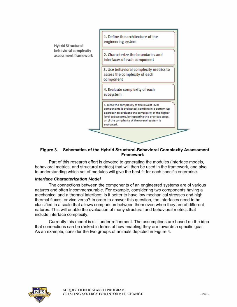
This framework has been built with flexibility in mind, meaning that the interface characterization model, the behavioral metric, and the structural metric are supposed to be plugged in according to the specific characteristics of the enterprise building the system, and the type of system. We have attempted to remove the majority of the subjectivity from the evaluation, since the level of accuracy depends heavily on the level of experience of the experts, but we want to retain the knowledge that any system architect has about the system that its enterprise is comfortable building. Two senior system architects are going to evaluate architectures differently, according to their experience and the experience of the people they worked with, thus naturally picking the best choice for the enterprise they work for. Just as likely, the framework can be adapted to rate as “better designed” the architectures having traits that the enterprise successfully implemented in past projects. Figure 3 shows a summary of the hybrid structural-behavioral framework.
^Åèìáëáíáçå=oÉëÉ~êÅÜ=mêçÖê~ãW=`êÉ~íáåÖ=póåÉêÖó=Ñçê=fåÑçêãÉÇ=`Ü~åÖÉ= - 240 -
Schematics of the Hybrid Structural-Behavioral Complexity Assessment Framework
Part of this research effort is devoted to generating the modules (interface models, behavioral metrics, and structural metrics) that will then be used in the framework, and also to understanding which set of modules will give the best fit for each specific enterprise.
Interface Characterization Model
The connections between the components of an engineered systems are of various natures and often incommensurable. For example, considering two components having a mechanical and a thermal interface: Is it better to have low mechanical stresses and high thermal fluxes, or vice versa? In order to answer this question, the interfaces need to be classified in a scale that allows comparison between them even when they are of different natures. This will enable the evaluation of many structural and behavioral metrics that include interface complexity.
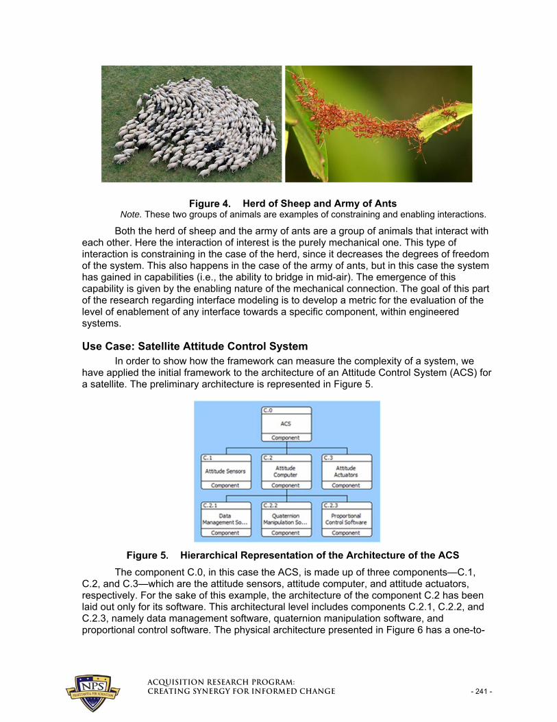
Currently this model is still under refinement. The assumptions are based on the idea that connections can be ranked in terms of how enabling they are towards a specific goal. As an example, consider the two groups of animals depicted in Figure 4.
^Åèìáëáíáçå=oÉëÉ~êÅÜ=mêçÖê~ãW=`êÉ~íáåÖ=póåÉêÖó=Ñçê=fåÑçêãÉÇ=`Ü~åÖÉ= - 241 -
Herd of Sheep and Army of Ants Note. These two groups of animals are examples of constraining and enabling interactions.
Both the herd of sheep and the army of ants are a group of animals that interact with each other. Here the interaction of interest is the purely mechanical one. This type of interaction is constraining in the case of the herd, since it decreases the degrees of freedom of the system. This also happens in the case of the army of ants, but in this case the system has gained in capabilities (i.e., the ability to bridge in mid-air). The emergence of this capability is given by the enabling nature of the mechanical connection. The goal of this part of the research regarding interface modeling is to develop a metric for the evaluation of the level of enablement of any interface towards a specific component, within engineered systems.
Use Case: Satellite Attitude Control System In order to show how the framework can measure the complexity of a system, we
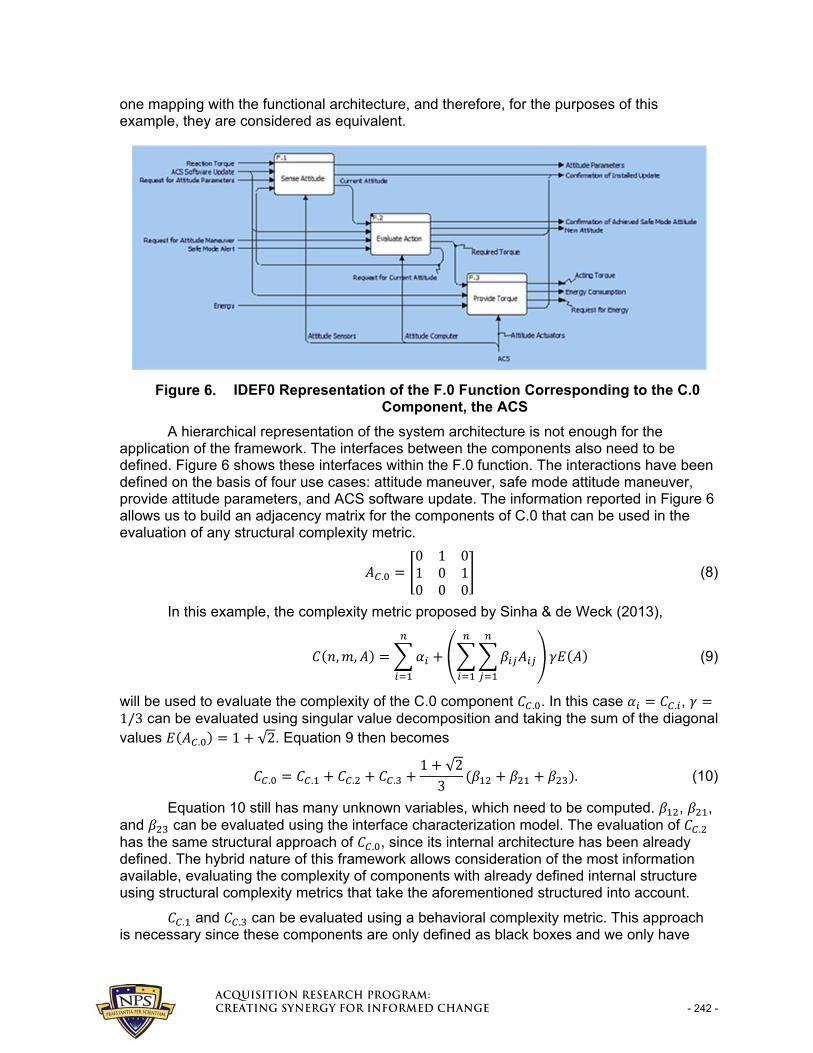
have applied the initial framework to the architecture of an Attitude Control System (ACS) for a satellite. The preliminary architecture is represented in Figure 5.
Hierarchical Representation of the Architecture of the ACS
The component C.0, in this case the ACS, is made up of three components—C.1, C.2, and C.3—which are the attitude sensors, attitude computer, and attitude actuators, respectively. For the sake of this example, the architecture of the component C.2 has been laid out only for its software. This architectural level includes components C.2.1, C.2.2, and C.2.3, namely data management software, quaternion manipulation software, and proportional control software. The physical architecture presented in Figure 6 has a one-to-
^Åèìáëáíáçå=oÉëÉ~êÅÜ=mêçÖê~ãW=`êÉ~íáåÖ=póåÉêÖó=Ñçê=fåÑçêãÉÇ=`Ü~åÖÉ= - 242 -
one mapping with the functional architecture, and therefore, for the purposes of this example, they are considered as equivalent.
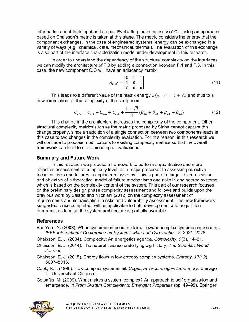
IDEF0 Representation of the F.0 Function Corresponding to the C.0 Component, the ACS
A hierarchical representation of the system architecture is not enough for the application of the framework. The interfaces between the components also need to be defined. Figure 6 shows these interfaces within the F.0 function. The interactions have been defined on the basis of four use cases: attitude maneuver, safe mode attitude maneuver, provide attitude parameters, and ACS software update. The information reported in Figure 6 allows us to build an adjacency matrix for the components of C.0 that can be used in the evaluation of any structural complexity metric.
.
0 1 01 0 10 0 0
(8)
In this example, the complexity metric proposed by Sinha & de Weck (2013),
, , (9)
will be used to evaluate the complexity of the C.0 component . . In this case . , 1/3 can be evaluated using singular value decomposition and taking the sum of the diagonal values . 1 √2. Equation 9 then becomes
. . . .1 √23
. (10)
Equation 10 still has many unknown variables, which need to be computed. , , and can be evaluated using the interface characterization model. The evaluation of . has the same structural approach of . , since its internal architecture has been already defined. The hybrid nature of this framework allows consideration of the most information available, evaluating the complexity of components with already defined internal structure using structural complexity metrics that take the aforementioned structured into account.
. and . can be evaluated using a behavioral complexity metric. This approach is necessary since these components are only defined as black boxes and we only have
^Åèìáëáíáçå=oÉëÉ~êÅÜ=mêçÖê~ãW=`êÉ~íáåÖ=póåÉêÖó=Ñçê=fåÑçêãÉÇ=`Ü~åÖÉ= - 243 -
information about their input and output. Evaluating the complexity of C.1 using an approach based on Chaisson’s metric is taken at this stage. The metric considers the energy that the component exchanges. In the case of engineered systems, energy can be exchanged in a variety of ways (e.g., chemical, data, mechanical, thermal). The evaluation of this exchange is also part of the interface characterization model under development in this research.
In order to understand the dependency of the structural complexity on the interfaces, we can modify the architecture of F.0 by adding a connection between F.1 and F.3. In this case, the new component C.O will have an adjacency matrix:
.
0 1 11 0 10 0 0
(11)
This leads to a different value of the matrix energy . 1 √3 and thus to a new formulation for the complexity of the component:
. . . .1 √33
(12)
This change in the architecture increases the complexity of the component. Other structural complexity metrics such as the metric proposed by Sinha cannot capture this change properly, since an addition of a single connection between two components leads in this case to two changes in the complexity evaluation. For this reason, in this research we will continue to propose modifications to existing complexity metrics so that the overall framework can lead to more meaningful evaluations.
Summary and Future Work In this research we propose a framework to perform a quantitative and more
objective assessment of complexity level, as a major precursor to assessing objective technical risks and failures in engineered systems. This is part of a larger research vision and objective of a theoretical model of failure mechanisms and risks in engineered systems, which is based on the complexity content of the system. This part of our research focuses on the preliminary design phase complexity assessment and follows and builds upon the previous work by Salado and Nilchiani (2012) on the complexity assessment of requirements and its translation in risks and vulnerability assessment. The new framework suggested, once completed, will be applicable to both development and acquisition programs, as long as the system architecture is partially available.
References Bar-Yam, Y. (2003). When systems engineering fails: Toward complex systems engineering.
IEEE International Conference on Systems, Man and Cybernetics, 2, 2021–2028.
Chaisson, E. J. (2004). Complexity: An energetics agenda. Complexity, 9(3), 14–21.
Chaisson, E. J. (2014). The natural science underlying big history. The Scientific World Journal.
Chaisson, E. J. (2015). Energy flows in low-entropy complex systems. Entropy, 17(12), 8007–8018.
Cook, R. I. (1998). How complex systems fail. Cognitive Technologies Laboratory. Chicago IL: University of Chigaco.
Cotsaftis, M. (2009). What makes a system complex? An approach to self organization and emergence. In From System Complexity to Emergent Properties (pp. 49–99). Springer.
^Åèìáëáíáçå=oÉëÉ~êÅÜ=mêçÖê~ãW=`êÉ~íáåÖ=póåÉêÖó=Ñçê=fåÑçêãÉÇ=`Ü~åÖÉ= - 244 -
DoD. (2006). Risk management guide for DoD acquisition. Washington, DC: Author.
Edmonds, B. (1995). What is complexity? The philosophy of complexity per se with application to some examples in evolution. The Evolution of Complexity.
Gell-Mann, M. (1995). What is complexity? Remarks on simplicity and complexity by the Nobel Prize-winning author of The Quark and the Jaguar. Complexity, 1(1), 16–19.
Gell-Mann, M. (2002). What is complexity? In Complexity and Industrial Clusters, 13–24. Springer.
Gell-Mann, M., & Lloyd, S. (1996). Information measures, effective complexity, and total information. Complexity, 2(1), 44–52.
Griffin, M. D. (2010). How do we fix system engineering? International Astronautical Congress.
Hazelrigg, G. A. (1998). A framework for decision-based engineering design. Journal of Mechanical Design, 120(4), 653–658.
Hessami, A. (1999). Risk management: A systems paradigm. Systems Engineering, 2(3), 156–167.
Kauffman, S. (2007). Beyond reductionism: Reinventing the sacred. Zygon, 42(4), 903–914.
Longo, G., Montevil, M., & Kauffman, S. (2012). No entailing laws, but enablement in the evolution of the biosphere. In Proceedings of the 14th Annual Conference Companion on Genetic and Evolutionary Computation, 1379–1392.
Madni, A. M. (2012). Elegant systems design: Creative fusion of simplicity and power. Systems Engineering, 15(3), 347–354.
McCabe, T. J. (1976). A complexity measure. IEEE Transactions on Software Engineering, (4), 308–320.
McCabe, T. J., & Butler, C. W. (1989). Design complexity measurement and testing. Communications of the ACM, 32(12), 1415–1425.
Merry, U., & Kassavin, N. (1995). Coping with uncertainty: Insights from the new sciences of chaos, self-organization, and complexity. Praeger/Greenwood.
Nilchiani, R., Mostashari, A., Rifkin, S., Bryzik, W., & Witus, G. (2013). Quantitative risk—Phase 1. Systems Engineering Research Center–University Affiliated Research Center.
Page, S. E. (1999). Computational models from A to Z. Complexity, 5(1), 35–41.
Pennock, M., & Haimes, Y. (2002). Principles and guidelines for project risk management. Systems Engineering, 89–108.
Salado, A., & Nilchiani, R. (2012). A framework to assess the impact of requirements on system complexity.
Salado, A., & Nilchiani, R. (2013a). Elegant space systems: How do we get there? In Proceedings of the IEEE Aerospace Conference (pp. 1–12). IEEE.
Salado, A., & Nilchiani, R. (2013b). Using Maslow’s hierarchy of needs to define elegance in system architecture. Procedia Computer Science, 16, 927–936.
Shannon, C. E. (1948). A mathematical theory of communication. The Bell System Technical Journal, 27(3), 379–423.
Sinha, K., & de Weck, O. L. (2012). Structural complexity metric for engineered complex systems and its application. Gain Competitive Advantage by Managing Complexity: Proceedings of the 14th International DSM Conference Kyoto, Japan, (pp. 181–194).
Sinha, K., & de Weck, O. L. (2013). A network-based structural complexity metric for engineered complex systems. IEEE International Systems Conference (SysCon) (pp. 426–430).

^Åèìáëáíáçå=oÉëÉ~êÅÜ=mêçÖê~ãW=`êÉ~íáåÖ=póåÉêÖó=Ñçê=fåÑçêãÉÇ=`Ü~åÖÉ= - 245 -
Wade, J., & Heydari, B. (2014). Complexity: Definition and reduction techniques. Proceedings of the Poster Workshop at the 2014 Complex Systems Design & Management International Conference (pp. 213–226).
Weaver, W. (1948). Science and complexity. American Scientist, 36(4), 536–544.
Willcox, K., Allaire, D., Deyst, J., He, C., & Sondecker, G. (2011). Stochastic process decision methods for complex-cyber-physical systems (Technical report, DTIC document).

^Åèìáëáíáçå=oÉëÉ~êÅÜ=mêçÖê~ã=dê~Çì~íÉ=pÅÜççä=çÑ=_ìëáåÉëë=C=mìÄäáÅ=mçäáÅó=k~î~ä=mçëíÖê~Çì~íÉ=pÅÜççä=RRR=aóÉê=oç~ÇI=fåÖÉêëçää=e~ää=jçåíÉêÉóI=`^=VPVQP=
www.acquisitionresearch.net
A Complex Systems Perspective of Risk Mitigation and Modeling in Development and Acquisition Programs
Dr. Roshanak Nilchiani Associate Professor School of Systems and Enterprises Stevens Institute of Technology
13th Annual Acquisition Research Symposium Acquisition Research Program Naval Postgraduate School
Antonio Pugliese PhD Student School of Systems and Enterprises Stevens Institute of Technology
Current Methodologies in Risk Assessment
Hybrid Structural-Behavioral Complexity Framework
Structural Complexity Metrics
Interface Characterization Model
Behavioral Complexity Metrics
Use Case: Satellite Attitude Control System
Modification of Existing Metrics
Summary and Future Work
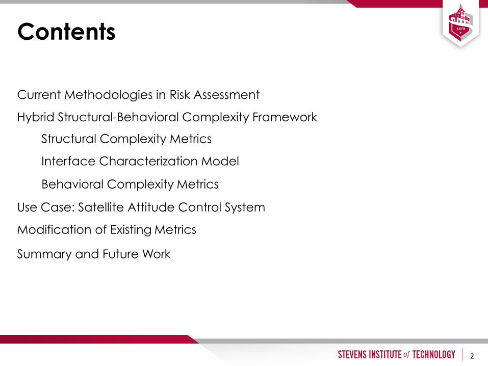
Contents
2
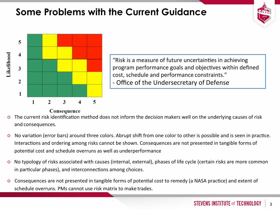
Some Problems with the Current Guidance
“Riskisameasureoffutureuncertain2esinachievingprogramperformancegoalsandobjec2veswithindefinedcost,scheduleandperformanceconstraints.”-OfficeoftheUndersecretaryofDefense
○ Thecurrentriskiden2fica2onmethoddoesnotinformthedecisionmakerswellontheunderlyingcausesofriskandconsequences.
○ Novaria2on(errorbars)aroundthreecolors.AbruptshiMfromonecolortootherispossibleandisseeninprac2ce.Interac2onsandorderingamongriskscannotbeshown.Consequencesarenotpresentedintangibleformsofpoten2alcostandscheduleoverrunsaswellasunderperformance
○ Notypologyofrisksassociatedwithcauses(internal,external),phasesoflifecycle(certainrisksaremorecommoninpar2cularphases),andinterconnec2onsamongchoices.
○ Consequencesarenotpresentedintangibleformsofpoten2alcosttoremedy(aNASAprac2ce)andextentofscheduleoverruns.PMscannotuseriskmatrixtomaketrades.
3
Different Approaches
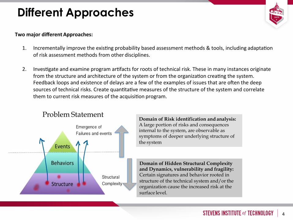
Problem Statement Domain of Risk identification and analysis: A large portion of risks and consequences internal to the system, are observable as symptoms of deeper underlying structure of the system
Domain of Hidden Structural Complexity and Dynamics, vulnerability and fragility: Certain signatures and behavior rooted in structure of the technical system and/or the organization cause the increased risk at the surface level.
TwomajordifferentApproaches:
1. Incrementallyimprovetheexis2ngprobabilitybasedassessmentmethods&tools,includingadapta2onofriskassessmentmethodsfromotherdisciplines.
2. Inves2gateandexamineprogramar2factsforrootsoftechnicalrisk.Theseinmanyinstancesoriginatefromthestructureandarchitectureofthesystemorfromtheorganiza2oncrea2ngthesystem.FeedbackloopsandexistenceofdelaysareafewoftheexamplesofissuesthatareoMenthedeepsourcesoftechnicalrisks.Createquan2ta2vemeasuresofthestructureofthesystemandcorrelatethemtocurrentriskmeasuresoftheacquisi2onprogram.
4
Research Approach
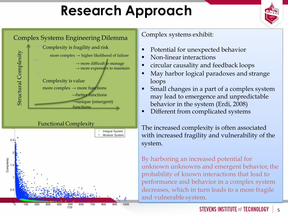
Complex systems exhibit: § Potential for unexpected behavior § Non-linear interactions § circular causality and feedback loops § May harbor logical paradoxes and strange
loops § Small changes in a part of a complex system
may lead to emergence and unpredictable behavior in the system (Erdi, 2008)
§ Different from complicated systems
The increased complexity is often associated with increased fragility and vulnerability of the system. By harboring an increased potential for unknown unknowns and emergent behavior, the probability of known interactions that lead to performance and behavior in a complex system decreases, which in turn leads to a more fragile and vulnerable system.
Stru
ctur
al C
ompl
exity
Complex Systems Engineering Dilemma Complexity is fragility and risk
more complex → higher likelihood of failure
→ more difficult to manage → more expensive to maintain
Complexity is value more complex → more functions
→better functions →unique (emergent) functions
Functional Complexity
5
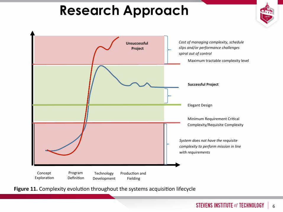
Figure11.Complexityevolu2onthroughoutthesystemsacquisi2onlifecycle
ElegantDesign
MinimumRequirementCri2calComplexity/RequisiteComplexity
Systemdoesnothavetherequisitecomplexitytoperformmissioninlinewithrequirements
SuccessfulProject
Costofmanagingcomplexity,scheduleslipsand/orperformancechallengesspiraloutofcontrol
Maximumtractablecomplexitylevel
UnsuccessfulProject
ConceptExplora2on
ProgramDefini2on
Technology Produc2onandDevelopment Fielding
Research Approach
6
ProblemComplexityandRequirements
©2013SaladoandNilchiani
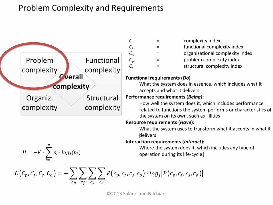
Overallcomplexity
Problemcomplexity
Organiz.complexity
Functionalcomplexity
Structuralcomplexity
C = complexityindexCf = func2onalcomplexityindexCo = organiza2onalcomplexityindexCp = problemcomplexityindexCs = structuralcomplexityindex
Func?onalrequirements(Do)Whatthesystemdoesinessence,whichincludeswhatitacceptsandwhatitdelivers
Performancerequirements(Being):Howwellthesystemdoesit,whichincludesperformancerelatedtofunc2onsthesystemperformsorcharacteris2csofthesystemonitsown,suchas–ili2es
Resourcerequirements(Have):Whatthesystemusestotransformwhatitacceptsinwhatitdelivers
Interac?onrequirements(Interact):Wherethesystemdoesit,whichincludesanytypeofopera2onduringitslife-cycle.
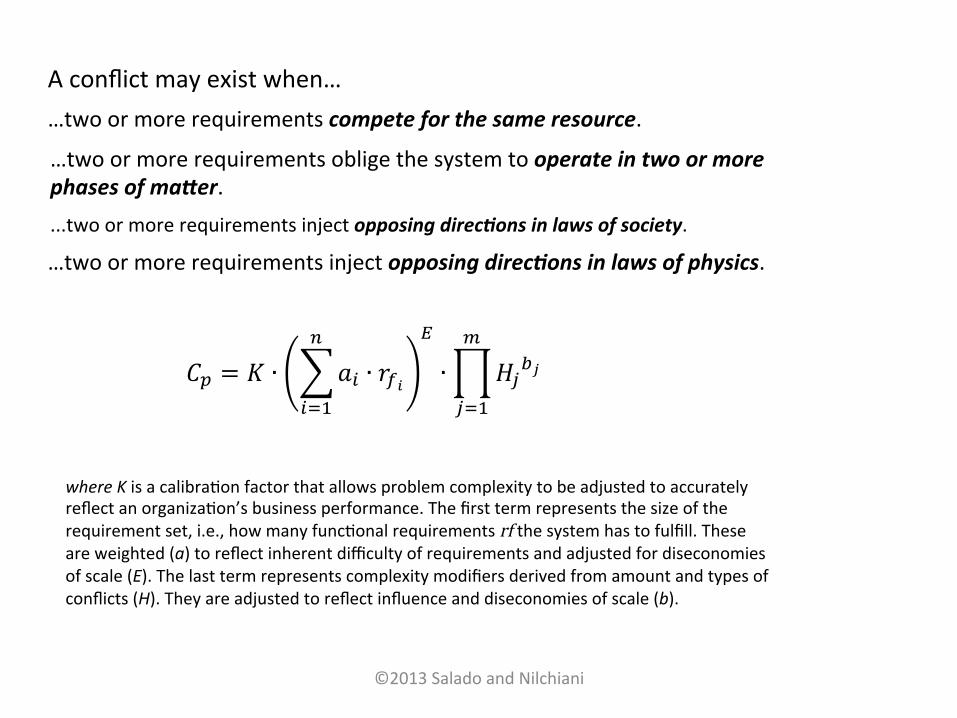
…twoormorerequirementscompeteforthesameresource.
…twoormorerequirementsinjectopposingdirec8onsinlawsofphysics.
...twoormorerequirementsinjectopposingdirec8onsinlawsofsociety.
…twoormorerequirementsobligethesystemtooperateintwoormorephasesofma<er.
Aconflictmayexistwhen…
©2013SaladoandNilchiani
!! = ! ∙ !! ∙ !!!!
!!!
!
∙ !!!!!
!!!
whereKisacalibra2onfactorthatallowsproblemcomplexitytobeadjustedtoaccuratelyreflectanorganiza2on’sbusinessperformance.Thefirsttermrepresentsthesizeoftherequirementset,i.e.,howmanyfunc2onalrequirementsrfthesystemhastofulfill.Theseareweighted(a)toreflectinherentdifficultyofrequirementsandadjustedfordiseconomiesofscale(E).Thelasttermrepresentscomplexitymodifiersderivedfromamountandtypesofconflicts(H).Theyareadjustedtoreflectinfluenceanddiseconomiesofscale(b).
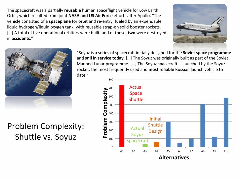
ThespacecraMwasapar2allyreusablehumanspaceflightvehicleforLowEarthOrbit,whichresultedfromjointNASAandUSAirForceeffortsaMerApollo.“Thevehicleconsistedofaspaceplanefororbitandre-entry,fueledbyanexpendableliquidhydrogen/liquidoxygentank,withreusablestrap-onsolidboosterrockets.[…]Atotaloffiveopera2onalorbiterswerebuilt,andofthese,twoweredestroyedinaccidents.”
“SoyuzisaseriesofspacecraMini2allydesignedfortheSovietspaceprogrammeands?llinservicetoday.[…]TheSoyuzwasoriginallybuiltaspartoftheSovietMannedLunarprogramme.[…]TheSoyuzspacecraMislaunchedbytheSoyuzrocket,themostfrequentlyusedandmostreliableRussianlaunchvehicletodate.”
ProblemComplexity:Shumlevs.Soyuz
ActualSpaceShu,le
ActualSoyuz
Spacecra1
Ini5alShu,leDesign
0
100
200
300
400
500
600
700
800
A1 A2 A3 A4 A5 A6 A7 A8 A9 A10
Prob
lemCom
plexity
Alterna2ves
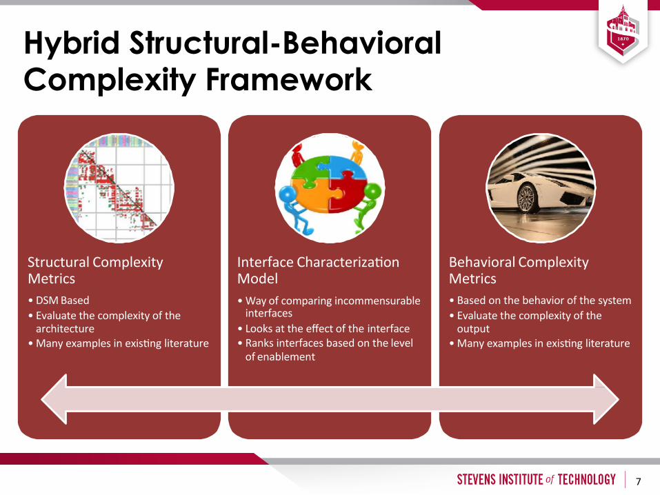
Hybrid Structural-Behavioral Complexity Framework
7
StructuralComplexityMetrics• DSMBased• Evaluatethecomplexityofthearchitecture
• Manyexamplesinexis2ngliterature
InterfaceCharacteriza2onModel• Wayofcomparingincommensurableinterfaces
• Looksattheeffectoftheinterface• Ranksinterfacesbasedonthelevelofenablement
BehavioralComplexityMetrics• Basedonthebehaviorofthesystem• Evaluatethecomplexityoftheoutput
• Manyexamplesinexis2ngliterature
8
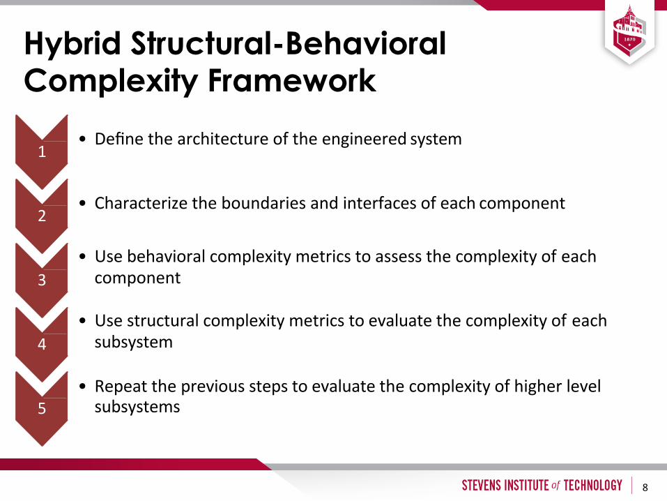
Hybrid Structural-Behavioral Complexity Framework
1• Definethearchitectureoftheengineeredsystem
2• Characterizetheboundariesandinterfacesofeachcomponent
3• Usebehavioralcomplexitymetricstoassessthecomplexityofeachcomponent
4• Usestructuralcomplexitymetricstoevaluatethecomplexityofeachsubsystem
5• Repeatthepreviousstepstoevaluatethecomplexityofhigherlevelsubsystems
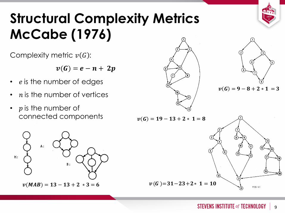
Complexity metric 𝑣 𝐺 :
𝒗 𝑮 = 𝒆 − 𝒏 + 𝟐𝒑
• 𝑒 is the number of edges
• 𝑛 is the number of vertices
• 𝑝 is the number of connected components
Structural Complexity Metrics McCabe (1976)
9
𝒗 𝑮 = 𝟗 − 𝟖 + 𝟐 ∗ 𝟏 = 𝟑
𝒗 𝑮 = 𝟏𝟗 − 𝟏𝟑 + 𝟐 ∗ 𝟏 = 𝟖
𝒗 (𝑮 )= 𝟑𝟏 − 𝟐𝟑 + 𝟐 ∗ 𝟏 = 𝟏𝟎 𝒗(𝑴𝑨𝑩) = 𝟏𝟑 − 𝟏𝟑 + 𝟐 ∗ 𝟑 = 𝟔
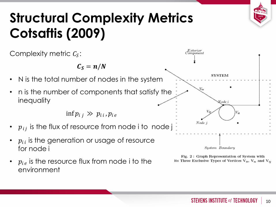
Structural Complexity Metrics Cotsaftis (2009)
10
Complexity metric 𝐶𝑆 :
𝑪𝑺 = 𝒏/𝑵
• N is the total number of nodes in the system
• n is the number of components that satisfy the inequality
inf 𝑝𝑖 𝑗 ≫ 𝑝𝑖 𝑖 , 𝑝𝑖 𝑒
• 𝑝𝑖 𝑗 is the flux of resource from node i to node j
• 𝑝𝑖 𝑖 is the generation or usage of resource for node i
• 𝑝𝑖 𝑒 is the resource flux from node i to the environment
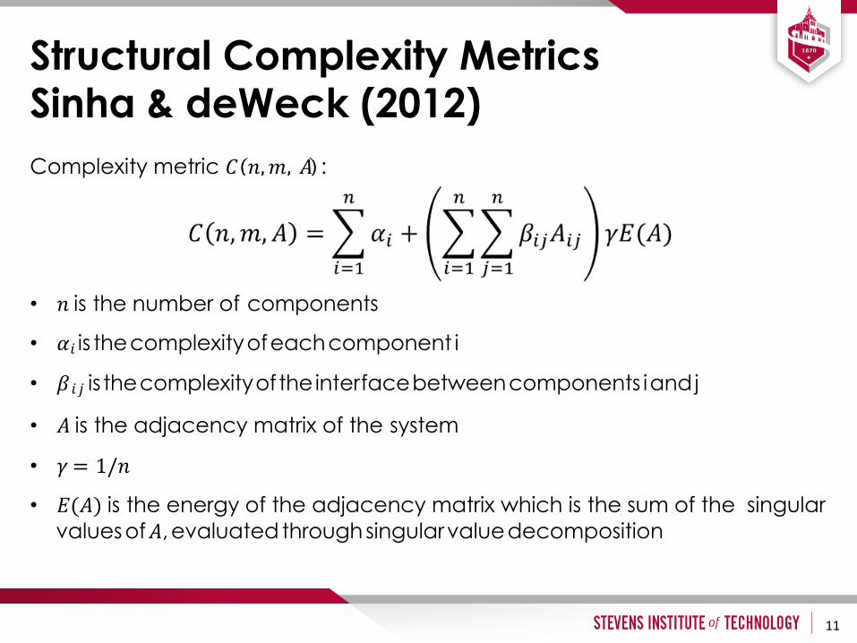
Complexity metric 𝐶 𝑛, 𝑚, 𝐴 :
• 𝑛 is the number of components
• 𝛼𝑖 is the complexity of each component i
• 𝛽𝑖 𝑗 is the complexity of the interface between components i and j
• 𝐴 is the adjacency matrix of the system
• 𝛾 = 1/𝑛
• 𝐸(𝐴) is the energy of the adjacency matrix which is the sum of the singular values of 𝐴, evaluated through singular value decomposition
Structural Complexity Metrics Sinha & deWeck (2012)
11
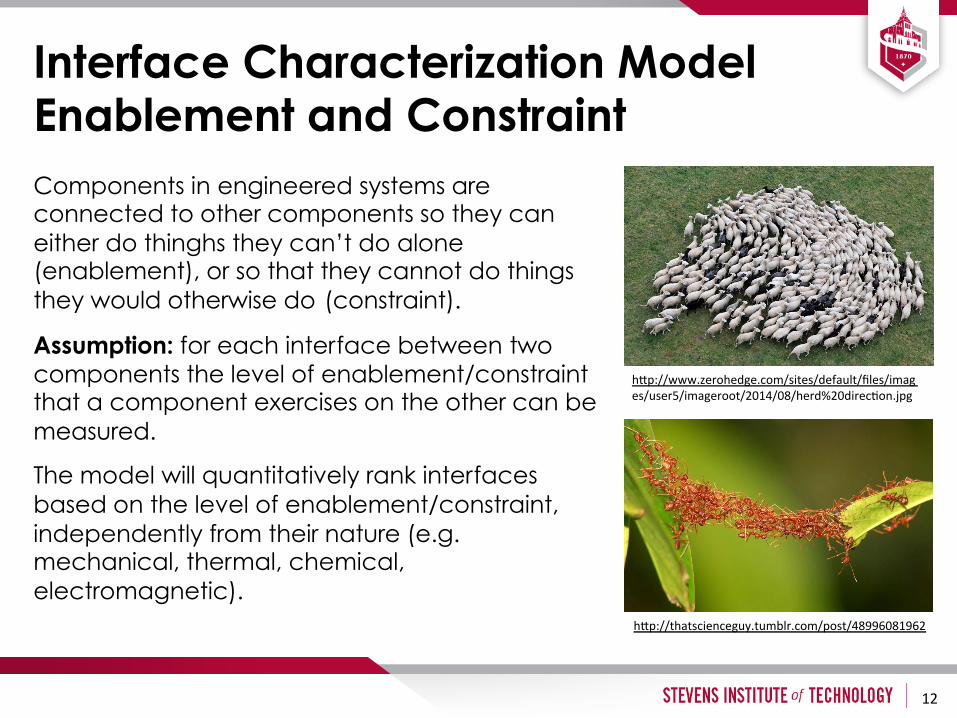
Components in engineered systems are connected to other components so they can either do thinghs they can’t do alone (enablement), or so that they cannot do things they would otherwise do (constraint).
Assumption: for each interface between two components the level of enablement/constraint that a component exercises on the other can be measured.
The model will quantitatively rank interfaces based on the level of enablement/constraint, independently from their nature (e.g. mechanical, thermal, chemical, electromagnetic).
Interface Characterization Model Enablement and Constraint
12
hmp://www.zerohedge.com/sites/default/files/images/user5/imageroot/2014/08/herd%20direc2on.jpg
hmp://thatscienceguy.tumblr.com/post/48996081962
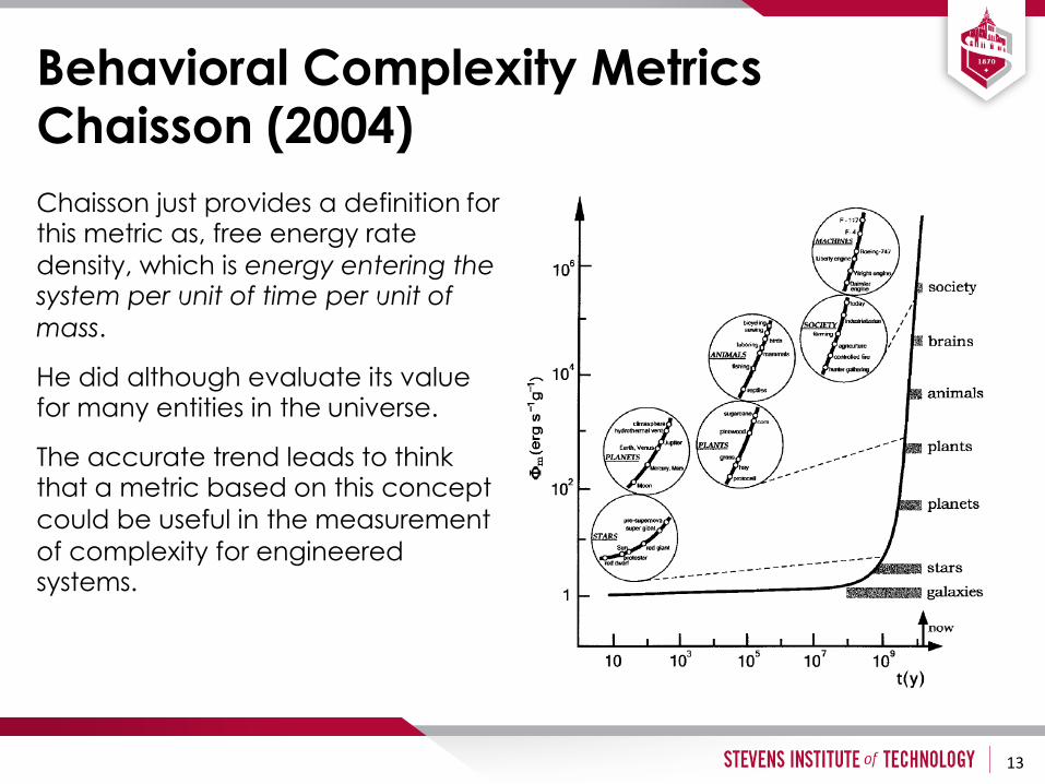
Chaisson just provides a definition for this metric as, free energy rate density, which is energy entering the system per unit of time per unit of mass.
He did although evaluate its value for many entities in the universe.
The accurate trend leads to think that a metric based on this concept could be useful in the measurement of complexity for engineered systems.
Behavioral Complexity Metrics Chaisson (2004)
13
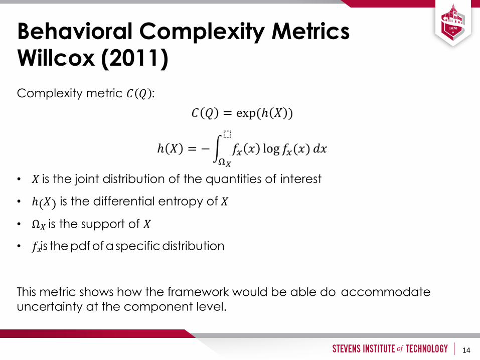
Complexity metric 𝐶 𝑄 :
• 𝑋 is the joint distribution of the quantities of interest
• ℎ 𝑋 is the differential entropy of 𝑋
• Ω𝑋 is the support of 𝑋
• 𝑓𝑥 is the pdf of a specific distribution This metric shows how the framework would be able do accommodate uncertainty at the component level.
Behavioral Complexity Metrics Willcox (2011)
14
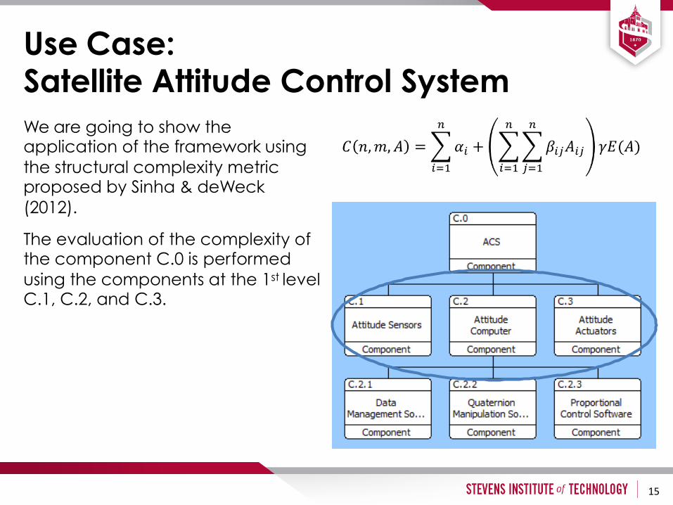
We are going to show the application of the framework using the structural complexity metric proposed by Sinha & deWeck (2012).
The evaluation of the complexity of the component C.0 is performed using the components at the 1st level C.1, C.2, and C.3.
Use Case: Satellite Attitude Control System
15
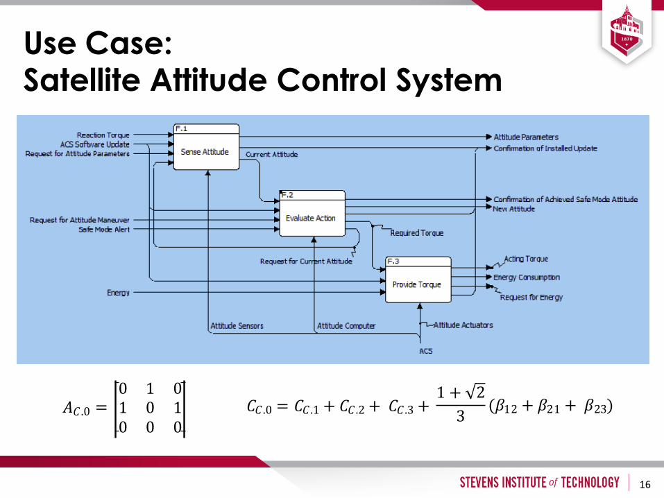
𝐴𝐶.0
0 1 0 = 1 0 1
0 0 0
16
Use Case: Satellite Attitude Control System
𝐶𝐶.0 = 𝐶𝐶.1 + 𝐶𝐶.2 + 𝐶𝐶.3 + 1 + 2
3 (𝛽12 + 𝛽21 + 𝛽23)
17
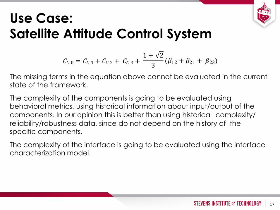
Use Case: Satellite Attitude Control System
𝐶𝐶.0 = 𝐶𝐶.1 + 𝐶𝐶.2 + 𝐶𝐶.3 + 1 + 2
3 (𝛽12 + 𝛽21 + 𝛽23)
The missing terms in the equation above cannot be evaluated in the current state of the framework.
The complexity of the components is going to be evaluated using behavioral metrics, using historical information about input/output of the components. In our opinion this is better than using historical complexity/reliability/robustness data, since do not depend on the history of the specific components.
The complexity of the interface is going to be evaluated using the interface characterization model.
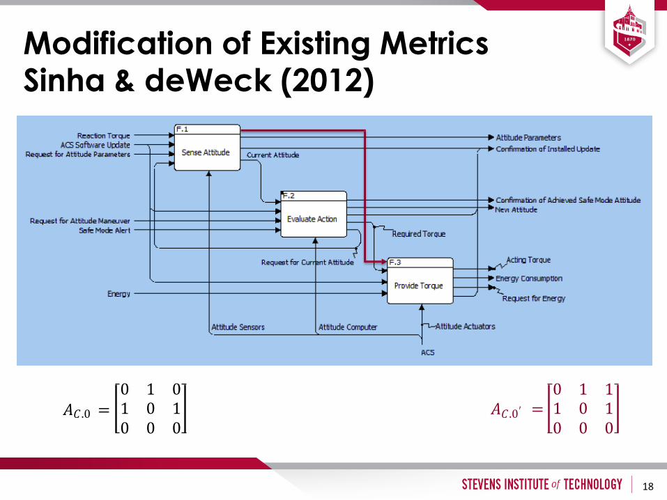
𝐴𝐶.0 = 0 1 0 1 0 1 0 0 0
18
Modification of Existing Metrics Sinha & deWeck (2012)
𝐴𝐶.0′ = 0 1 1 1 0 1 0 0 0
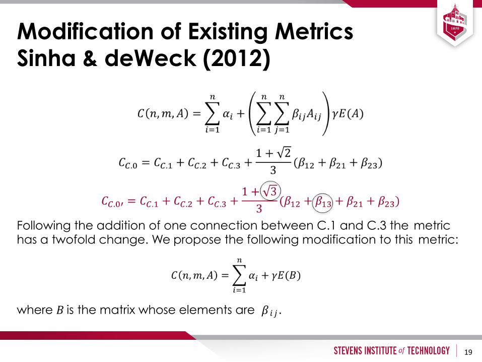
Following the addition of one connection between C.1 and C.3 the metric has a twofold change. We propose the following modification to this metric:
where 𝐵 is the matrix whose elements are 𝛽𝑖 𝑗 .
19
Modification of Existing Metrics Sinha & deWeck (2012)
Summary and Future Work
In this work we introduced the Hybrid Structural-Behavioral Complexity Framework.
The framework backbone has been defined, but its modules are yet to be developed.
Some modules are to be developed by modifying existing complexity metrics, while others are to be developed ex novo.
Future work will focus on the development of those modules and the validation of the framework using real data.
20

Thank you for your attention
Questions?

BackupSlidesExample:DARPAF6Program
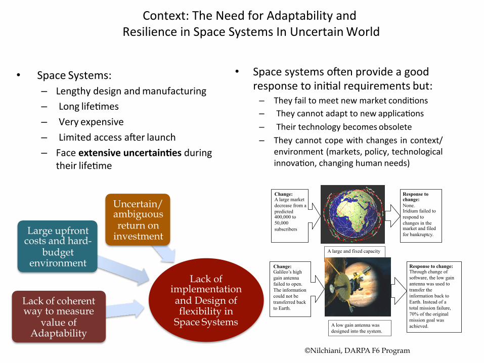
Context:TheNeedforAdaptabilityandResilienceinSpaceSystemsInUncertainWorld
• SpaceSystems:– Lengthydesignandmanufacturing– Longlife2mes– Veryexpensive– LimitedaccessaMerlaunch– Faceextensiveuncertain?esduring
theirlife2me
• SpacesystemsoMenprovideagoodresponsetoini2alrequirementsbut:
– Theyfailtomeetnewmarketcondi2ons– Theycannotadapttonewapplica2ons– Theirtechnologybecomesobsolete– Theycannotcopewithchangesincontext/
environment(markets,policy,technologicalinnova2on,changinghumanneeds)
Lack of implementation and Design of flexibility in
Space Systems
Large upfront costs and hard-
budget environment
Uncertain/ ambiguous return on
investment
Lack of coherent way to measure
value of Adaptability
Change: A large market decrease from a predicted 400,000 to 50,000 subscribers
Response to change: None. Iridium failed to respond to changes in the market and filed for bankruptcy.
A large and fixed capacity
Change: Galileo’s high gain antenna failed to open. The information could not be transferred back to Earth.
Response to change: Through change of software, the low gain antenna was used to transfer the information back to Earth. Instead of a total mission failure, 70% of the original mission goal was achieved. A low gain antenna was
designed into the system.
©Nilchiani, DARPA F6 Program
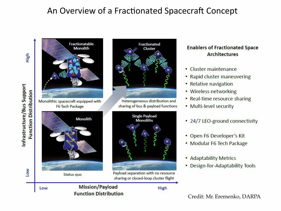
AnOverviewofaFrac2onatedSpacecraMConcept
Credit: Mr. Eremenko, DARPA
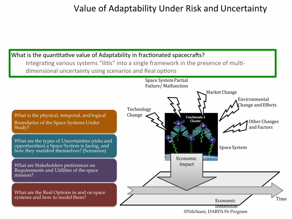
ValueofAdaptabilityUnderRiskandUncertainty
Whatisthequan2ta2vevalueofAdaptabilityinfrac2onatedspacecraMs?Integra2ngvarioussystems“ili2s”intoasingleframeworkinthepresenceofmul2-dimensionaluncertaintyusingscenariosandRealop2ons
Time
SpaceSystem
SpaceSystemPartialFailure/Malfunction
MarketChange
TechnologyChange
EnvironmentalChangeandEffects
EconomicImpact
OtherChangesandFactors
What is the physical, temporal, and logical Boundaries of the Space Systems Under Study?
What are the types of Uncertainties (risks and opportunities) a Space System is facing, and how they manifest themselves? (Scenarios)
What are Stakeholders preferences on Requirements and Utilities of the space mission?
What are the Real Options in and on space systems and how to model them?
EconomicDimension
©Nilchiani, DARPA F6 Program
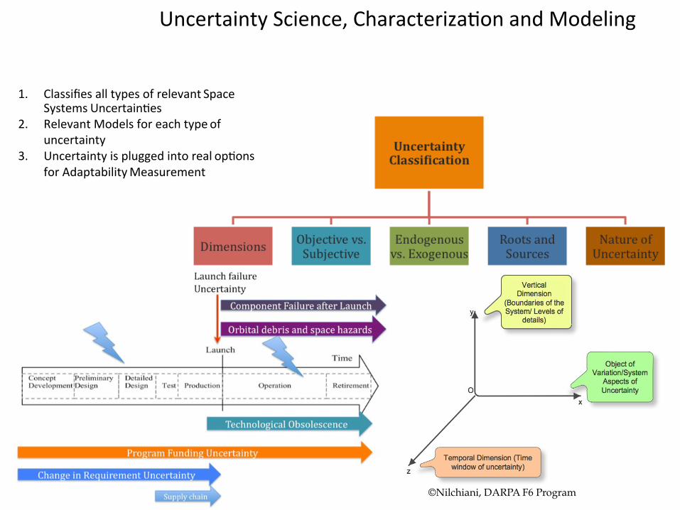
UncertaintyScience,Characteriza2onandModeling
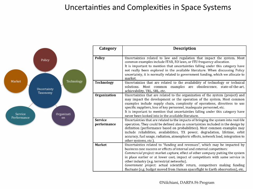
1. ClassifiesalltypesofrelevantSpaceSystemsUncertain2es
2. RelevantModelsforeachtypeofuncertainty
3. Uncertaintyispluggedintorealop2onsforAdaptabilityMeasurement
©Nilchiani, DARPA F6 Program
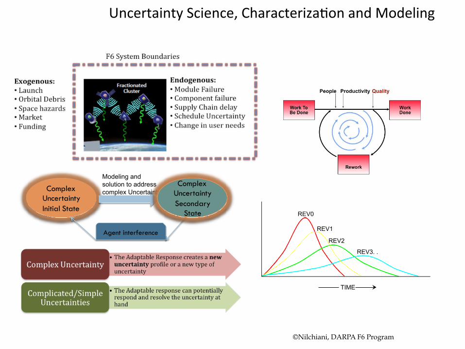
UncertaintyScience,Characteriza2onandModeling
Complex Uncertainty Initial State
Modeling and solution to address complex Uncertainty
Agent interference
Complex Uncertainty Secondary
State REV0
REV3. .
REV1
REV2
TIME
©Nilchiani, DARPA F6 Program

Uncertain2esandComplexi2esinSpaceSystems
Preliminary ModifiedDesign DesignRequirements Requirements
¨ Modeling Single Complex Uncertainty
F6ProjectRequirementUncertain2es
FundingUncertainty
CostStakeholdersInputs
ScheduleUncertaintyLag
Lag
Lag
RequirementUncertaintyismainlyafunc2onofchanginguserandstakeholdersneed,fundinguncertainty,andincompleteorunclearsetofini2alrequirements.Therearedelaysinrequirementgatheringandclassifica2onandpriori2za2onprocessandseveralloopsofitera2onsthataffectcostandprojectscheduledrama2cally
©Nilchiani, DARPA F6 Program
Correla2onMatrixofSpaceSystemsRelatedUncertain2es
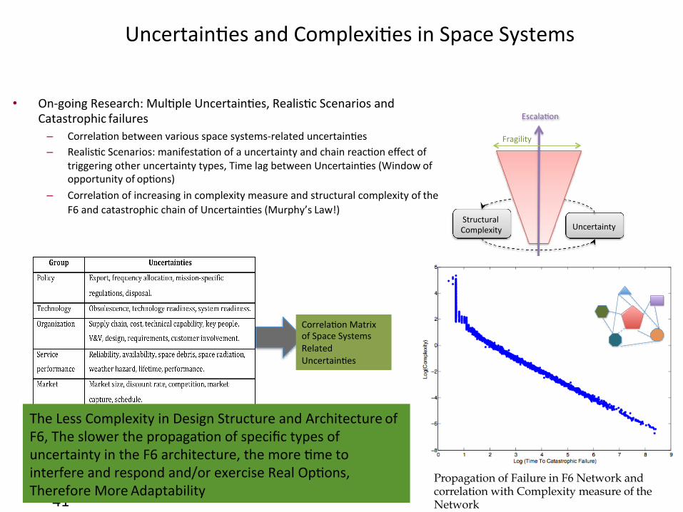
Uncertain2esandComplexi2esinSpaceSystems
41
• On-goingResearch:Mul2pleUncertain2es,Realis2cScenariosandCatastrophicfailures
– Correla2onbetweenvariousspacesystems-relateduncertain2es– Realis2cScenarios:manifesta2onofauncertaintyandchainreac2oneffectof
triggeringotheruncertaintytypes,TimelagbetweenUncertain2es(Windowofopportunityofop2ons)
– Correla2onofincreasingincomplexitymeasureandstructuralcomplexityoftheF6andcatastrophicchainofUncertain2es(Murphy’sLaw!)
StructuralComplexity Uncertainty
Escala2on
Fragility
Propagation of Failure in F6 Network and correlation with Complexity measure of the Network
TheLessComplexityinDesignStructureandArchitectureofF6,Theslowerthepropaga2onofspecifictypesofuncertaintyintheF6architecture,themore2metointerfereandrespondand/orexerciseRealOp2ons,ThereforeMoreAdaptability
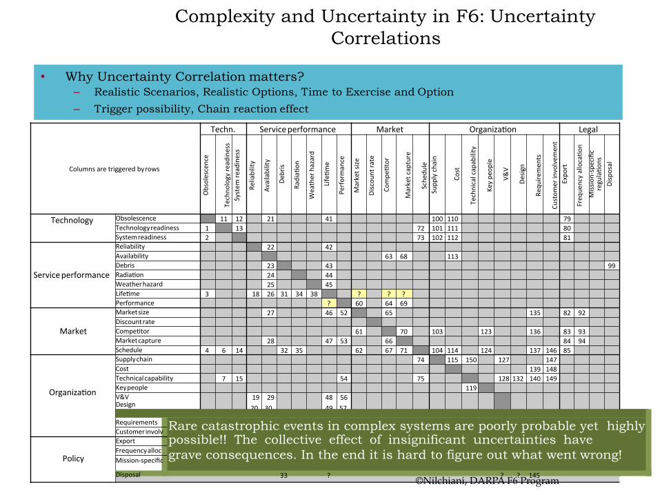
Complexity and Uncertainty in F6: Uncertainty Correlations
• Why Uncertainty Correlation matters? – Realistic Scenarios, Realistic Options, Time to Exercise and Option
– Trigger possibility, Chain reaction effect
2030 4957 1299 17 363739 ? 58 77 116120 130133 96
ement 781051171211251311341415 10 40 55 107106118122126 142
a2on ?108 143
regula2ons ? ? ? ? ? ? ? ? ? ? ? ? ? ? ? ? 144? 88
Columnsaretriggeredbyrows
Techn. Serviceperformance Market Organiza2on Legal
Obsolescence
Techno
logyre
adiness
System
readiness
Reliability
Availability
Debris
Radia2
on
Weatherhazard
Life2m
e
Performance
Marketsize
Discou
ntra
te
Compe
2tor
Marketcapture
Sche
dule
Supp
lychain
Co
st
Technicalcapability
Ke
ype
ople
V&
V
Desig
n
Requ
iremen
ts
Cu
stom
erinvolvem
ent
Expo
rt
Freq
uencyalloca2o
n
Mission-specific
regula2o
ns
Disposal
Technology Obsolescence 11 12 21 41 100 110 79Technologyreadiness 1 13 72 101 111 80Systemreadiness 2 73 102 112 81
Serviceperformance
Reliability 22 42Availability 63 68 113Debris 23 43 99Radia2on 24 44Weatherhazard 25 45Life2me 3 18 26 31 34 38 ? ? ?Performance ? 60 64 69
Market
Marketsize 27 46 52 65 135 82 92DiscountrateCompe2tor 61 70 103 123 136 83 93Marketcapture 28 47 53 66 84 94Schedule 4 6 14 32 35 62 67 71 104 114 124 137 146 85
Organiza2on
Supplychain 74 115 150 127 147Cost 139 148Technicalcapability 7 15 54 75 128 132 140 149Keypeople 119V&VDesign
19 29 48 56
Requirements Rare catastrophic events in complex systems are poorly probable yet highly possible!! The collective effect of insignificant uncertainties have grave consequences. In the end it is hard to figure out what went wrong!
Customerinvolv
Policy
ExportFrequencyallocMission-specific
Disposal 33 ? ? ? 145©Nilchiani, DARPA F6 Program
Uncertain2esandComplexi2esinSpaceSystems
©Nilchiani, DARPA F6 Program
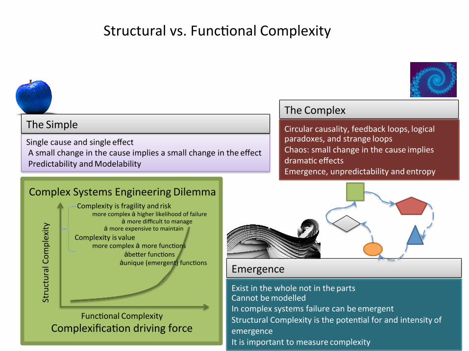
Structuralvs.Func2onalComplexity
SinglecauseandsingleeffectAsmallchangeinthecauseimpliesasmallchangeintheeffectPredictabilityandModelability
Circularcausality,feedbackloops,logicalparadoxes,andstrangeloopsChaos:smallchangeinthecauseimpliesdrama2ceffectsEmergence,unpredictabilityandentropy
ExistinthewholenotinthepartsCannotbemodelledIncomplexsystemsfailurecanbeemergentStructuralComplexityisthepoten2alforandintensityofemergenceItisimportanttomeasurecomplexity
TheSimpleTheComplex
Emergence
StructuralCom
plexity
ComplexSystemsEngineeringDilemmaComplexityisfragilityandrisk
morecomplexà higherlikelihoodoffailureà moredifficulttomanage
à moreexpensivetomaintainComplexityisvalue
morecomplexà morefunc2onsàbemerfunc2ons
àunique(emergent)func2ons
Func2onalComplexityComplexifica2ondrivingforce
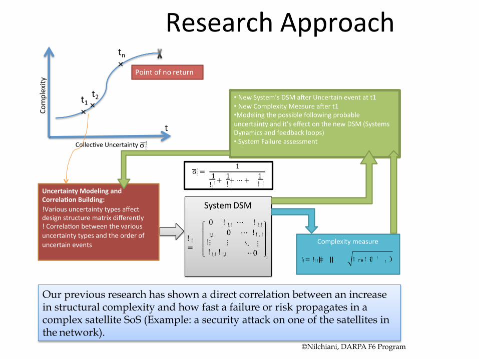
ResearchApproachCo
mplexity
Pointofnoreturn
×
t2t1×
Collec2veUncertaintyσ! !
tn×
UncertaintyModelingandCorrela?onBuilding:!Variousuncertaintytypesaffectdesignstructurematrixdifferently!Correla2onbetweenthevariousuncertaintytypesandtheorderofuncertainevents
! ! σ =
1
! + ! + ⋯ + 1 1 1 !! !! ! !
!
SystemDSM
! ! =
0
! !,!
! !,! ⋯ ! !,! 0 ⋯ ! ! , !
⋮ ⋮ ⋱ ⋮ ! !,! ! !,! ⋯ 0 !
Complexitymeasure
!! = !! ! = ! ! !"# ! !! !
• NewSystem’sDSMaMerUncertaineventatt1• NewComplexityMeasureaMert1•Modelingthepossiblefollowingprobableuncertaintyandit’seffectonthenewDSM(SystemsDynamicsandfeedbackloops)• SystemFailureassessment
t
Our previous research has shown a direct correlation between an increase in structural complexity and how fast a failure or risk propagates in a complex satellite SoS (Example: a security attack on one of the satellites in the network).
©Nilchiani, DARPA F6 Program
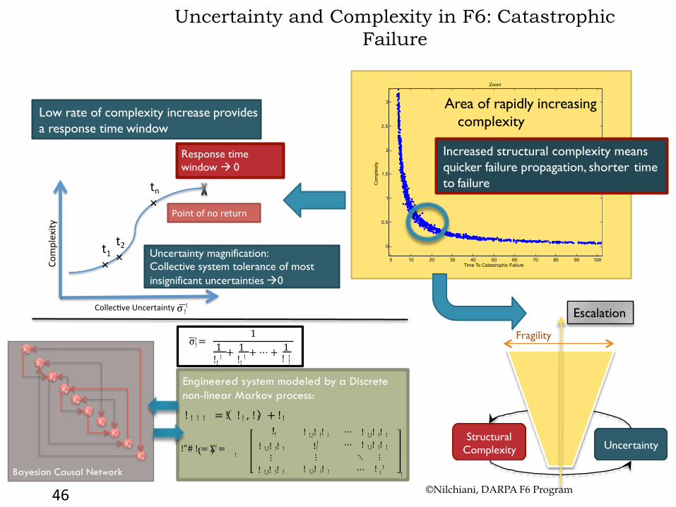
Uncertainty and Complexity in F6: Catastrophic Failure
46
Area of rapidly increasing complexity
0 10 20 30 80 90 100
0
0.5
1
1.5
2
2.5
3
40 50 60 70 Time To Catastrophic Failure
Com
plex
ity
Zoom
Complexity
Pointofnoreturn
t1×
t2×
Collec2veUncertaintyσ ! !
tn×
Response time window à 0
Low rate of complexity increase provides a response time window
Uncertainty magnification: Collective system tolerance of most insignificant uncertainties à0
Structural Complexity Uncertainty
Fragility
Escalation
Bayesian Causal Network
X1
X2
X3X4
X4X5
X6X7
X8X9
Engineered system modeled by a Discrete non-linear Markov process:
!"# !! = Σ! = !
! ! ! ! = ! ! ! , ! ! + ! !
!! !
!
⋯ ⋯ ! !,!! !! !
⋮ ! !,!! !! !
! !,!! !! !
!! ⋮
! !,!! !! !
! !,!! !! !
! !,!! !! !
⋱ ⋮ ⋯ ! ! !
!
! σ! = 1
1 + 1 + ⋯ + 1 !! !! ! !
! ! !
Increased structural complexity means quicker failure propagation, shorter time to failure
©Nilchiani, DARPA F6 Program
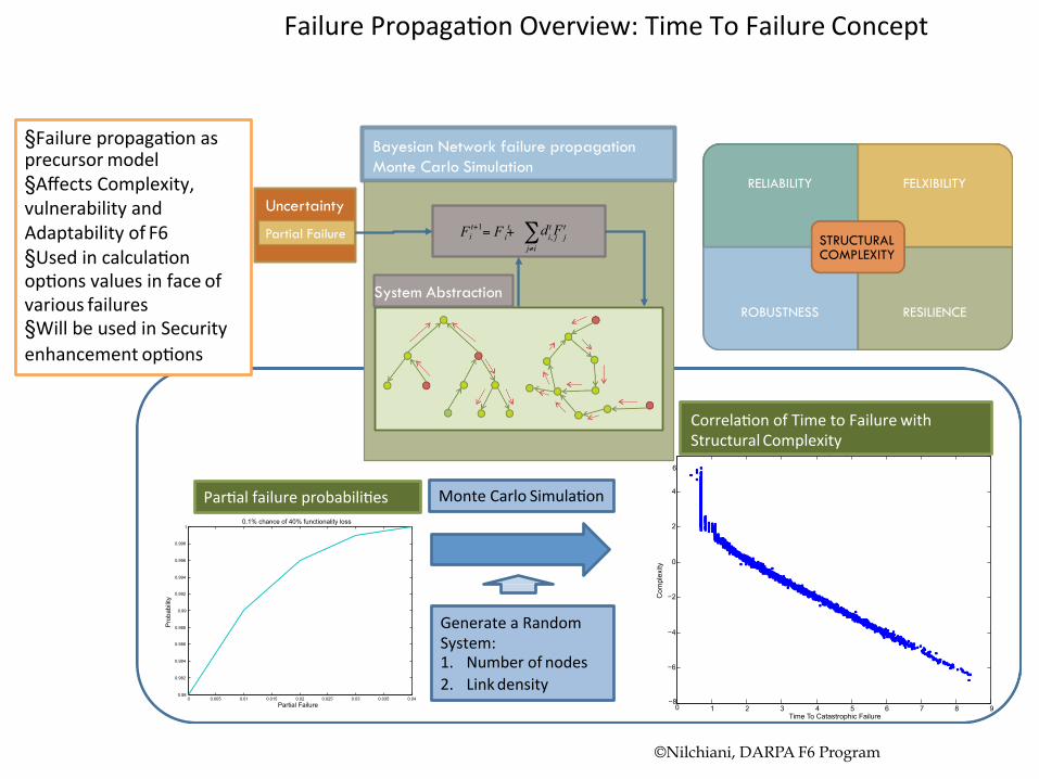
FailurePropaga2onOverview:TimeToFailureConcept
RELIABILITY FELXIBILITY
ROBUSTNESS RESILIENCE
STRUCTURAL COMPLEXITY
0 0.005 0.01 0.035 0.04 0.98
0.982
0.984
0.986
0.988
0.99
0.992
0.994
0.996
0.998
1
0.015 0.02 0.025 0.03 Partial Failure
Pro
babi
lity
0.1% chance of 40% functionality loss
1 2 3 6 7 8 9 −8
0
−6
−4
−2
0
2
4
6
Com
plex
ity
4 5 Time To Catastrophic Failure
Log−Log
Par2alfailureprobabili2es
Correla2onofTimetoFailurewithStructuralComplexity
MonteCarloSimula2on
GenerateaRandomSystem:1. Numberofnodes2. Linkdensity
Uncertainty
Bayesian Network failure propagation Monte Carlo Simulation
t+1 i Fi = F + i, j j t d t Ft ∑
j≠i Partial Failure
System System Abstraction
§ Failurepropaga2onasprecursormodel§ AffectsComplexity,vulnerabilityandAdaptabilityofF6§ Usedincalcula2onop2onsvaluesinfaceofvariousfailures§ WillbeusedinSecurityenhancementop2ons
©Nilchiani, DARPA F6 Program
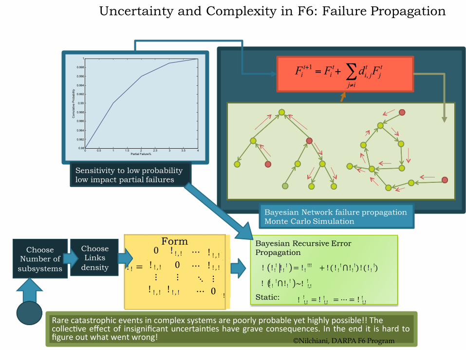
Uncertainty and Complexity in F6: Failure Propagation
t+1 t Fi = Fi + d F i, j j t t
j≠i ∑
0 0.5 1 1.5 2.5 3 3.5 4 0.98
0.992
0.99
0.988
0.986
0.984
0.982
0.994
0.996
0.998
1
2 Partial Failure%
Com
ulat
ive
Pro
babi
lity
Sensitivity to low probability low impact partial failures
Bayesian Network failure propagation Monte Carlo Simulation
Bayesian Recursive Error Propagation
! ! !,! !,! !,! = ! ! = ⋯ = ! !
! ! !!! ! ! ! ! ! ! ! ! = ! ! + ! ( ! ! ⋂!! ) ! ( ! ! )
Form 0 ! ! , !
⋯
! ! , !
! ! = ! ! , ! 0 ⋮ ⋮
⋯ ⋱
! ! , !
⋮ ! ! , ! ! ! , ! ⋯ 0
!
! ! ! ⋂!!
Static:
! ! ~! !,! !
Choose Number of subsystems
Choose Links
density
Rarecatastrophiceventsincomplexsystemsarepoorlyprobableyethighlypossible!!Thecollec2veeffectof insignificantuncertain2eshavegraveconsequences. Intheend it ishardtofigureoutwhatwentwrong! ©Nilchiani, DARPA F6 Program
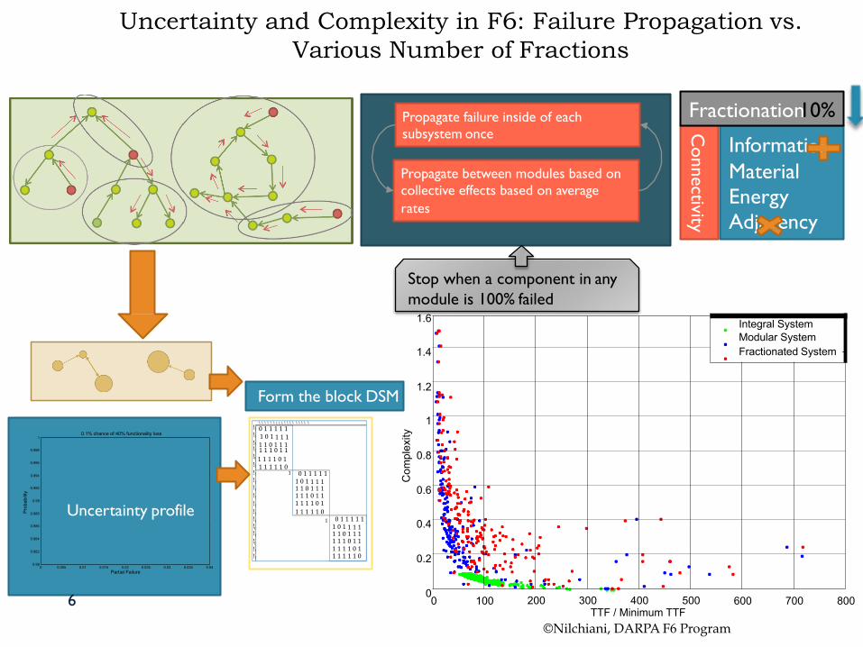
Uncertainty and Complexity in F6: Failure Propagation vs. Various Number of Fractions
6
Propagate failure inside of each subsystem once
Propagate between modules based on collective effects based on average rates
Stop when a component in any module is 100% failed
0 100 600 700 800 0
0.2
0.4
0.6
0.8
1
1.2
1.6
1.4
Com
plex
ity
Integral System Modular System Fractionated System
0 0.98
0.982
0.984
0.986
0.988
0.99
0.992
0.994
0.996
0.998
1
0.005 0.01 0.015 0.02 0.025 0.03 0.035 0.04 Partial Failure
Pro
babi
lity
0.1% chance of 40% functionality loss
Informati on Material Energy Adjacency
Connectivity
Fractionation10%
Form the block DSM
1 0 1 1 1 1
!! !! !! !! !! !! !! !! !! !! !! !! !! !! !! !! !! !!
!! 0 1 1 1 1 1 !!
!! 1 1 0 1 1 1 !! 1 1 1 0 1 1 ! ! 1 1 1 1 0 1 !! 1 1 1 1 1 0 !! !! !! !! !! !! !! ! ! !! ! ! !! !!
1 0 1 1 1 1 1 1 0 1 1 1 1 1 1 0 1 1 1 1 1 1 0 1 1 1 1 1 1 0
1 0 1 1 1 1 1 1 0 1 1 1 1 1 1 0 1 1 1 1 1 1 0 1 1 1 1 1 1 0
1 0 1 1 1 1 1
1 0 1 1 1 1 1
Uncertainty profile
200 300 400 500 TTF / Minimum TTF
©Nilchiani, DARPA F6 Program
50
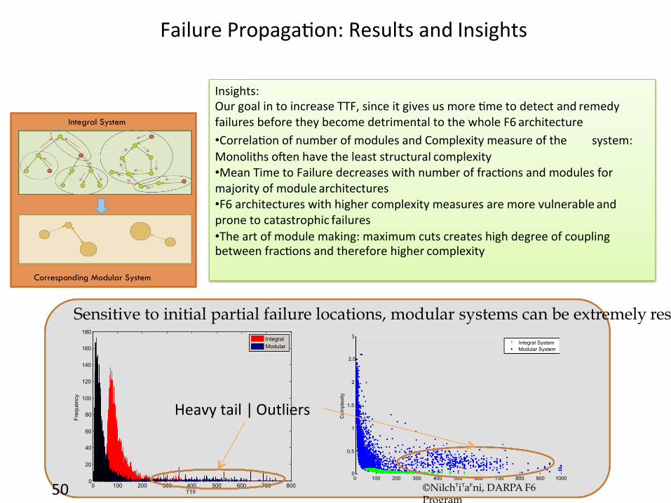
Integral System
Corresponding Modular System
100 200 300 400 500 600 700 800 900 1000 0 0
0.5
1
1.5
2
3 C
ompl
exity
Integral System Modular System
0 100 200 300 500 600 700 800 0
20
40
60
80
100
120
2.5 140
160
180
400 TTF
Freq
uenc
y
Integral Modular
Heavytail|Outliers
Sensitive to initial partial failure locations, modular systems can be extremely res
FailurePropaga2on:ResultsandInsights
Insights:OurgoalintoincreaseTTF,sinceitgivesusmore2metodetectandremedyfailuresbeforetheybecomedetrimentaltothewholeF6architecture• Correla2onofnumberofmodulesandComplexitymeasureofthe system:MonolithsoMenhavetheleaststructuralcomplexity• MeanTimetoFailuredecreaseswithnumberoffrac2onsandmodulesformajorityofmodulearchitectures• F6architectureswithhighercomplexitymeasuresaremorevulnerableandpronetocatastrophicfailures• Theartofmodulemaking:maximumcutscreateshighdegreeofcouplingbetweenfrac2onsandthereforehighercomplexity
©NilchTiTaFni, DARPA F6 Program
Integral
0 0 10 20 30 40
0.1
0.2
0.5
0.6
0.7
0.8
0.9
1
50 60 70 80 90 100 Time
Failu
re G
row
th%
Modular
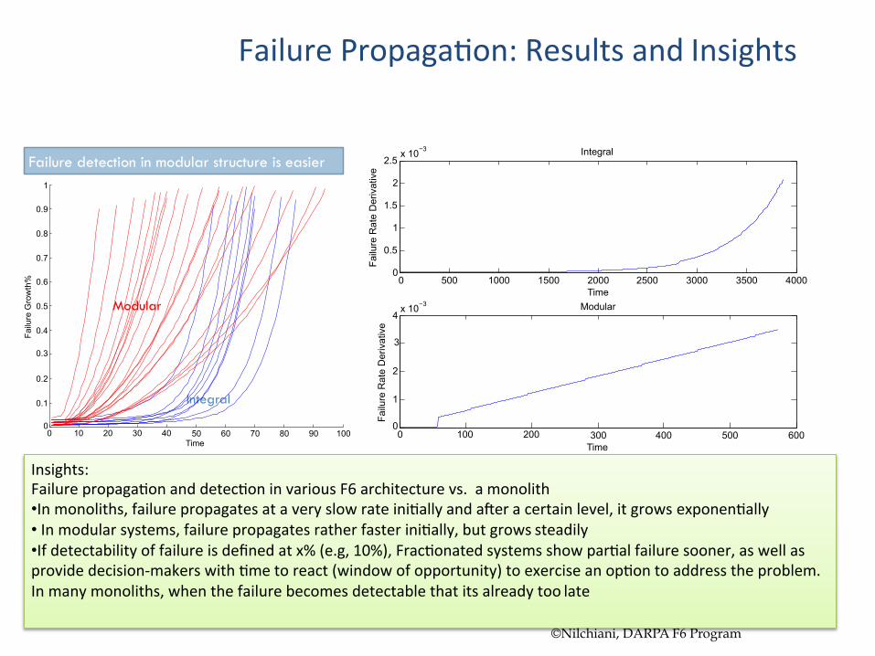
Failure detection in modular structure is easier
0 500 1000 1500 2500 3000 3500 4000 0
0.5
1
1.5
2
2.5 x 10 −3
Failu
re R
ate
Der
ivat
ive
Integral
0 0 100 200
1
2
0.4 3
0.3
4 x 10 −3
Failu
re R
ate
Der
ivat
ive
2000 Time
Modular
300 400 500 600 Time
Insights:Failurepropaga2onanddetec2oninvariousF6architecturevs.amonolith• Inmonoliths,failurepropagatesataveryslowrateini2allyandaMeracertainlevel,itgrowsexponen2ally• Inmodularsystems,failurepropagatesratherfasterini2ally,butgrowssteadily• Ifdetectabilityoffailureisdefinedatx%(e.g,10%),Frac2onatedsystemsshowpar2alfailuresooner,aswellasprovidedecision-makerswith2metoreact(windowofopportunity)toexerciseanop2ontoaddresstheproblem.Inmanymonoliths,whenthefailurebecomesdetectablethatitsalreadytoolate
FailurePropaga2on:ResultsandInsights
©Nilchiani, DARPA F6 Program