MECH 4810 Energy Conversions

DRAFT REPORT

Nova Scotia Wind Turbine Project Team # 2

Maigoro Yunana

James Gough

Kyle Kearse

Submitted: March 8th, 2016

1

Table of Contents

1.0 Introduction .............................................................................................................. 4

2.0 Wind Energy ............................................................................................................ 5

3.0 Site Selection Analysis ............................................................................................ 6

4.0 Turbine Selection ................................................................................................... 12

4.1. Offshore wind turbine support structure ................................................................ 18

5.0 Wave conditions..................................................................................................... 20

6.0 Finances ................................................................................................................. 26

7.0 References .............................................................................................................. 28

2

List of Tables

Table 1 - Basic parameters for wind turbine classes......................................................... 12

Table 2: Yarmouth Histogram .......................................................................................... 16

3

List of Figures

Figure 1: Wind shear Profile (van Der Tempel, 2006) ....................................................... 5 Figure 2: Nova Scotia transmission and distribution map .................................................. 7

Figure 3: Sable Island bathymetric chart (National Oceanic and Atmospheric

Administration) ................................................................................................................... 8 Figure 4: Yarmouth and Shelburne bathymetric (National Oceanic and Atmospheric

Administration) ................................................................................................................... 8 Figure 5: Daily Average Speed Variation ........................................................................... 9

Figure 6: Site Monthly Average ....................................................................................... 10 Figure 7: Site Raleigh Distribution ................................................................................... 11 Figure 8: Annual Wind Energy Available ........................................................................ 11

Figure 9: Turbulence intensity for the normal turbulence model ..................................... 13 Figure 10: E-126 calculated power curve ......................................................................... 14 Figure 11: Wind farm layout............................................................................................. 17 Figure 12: Yarmouth Wind Rose ...................................................................................... 18

Figure 13: Monopile support structure ............................................................................. 19 Figure 14: Score protection of a monopile ....................................................................... 20

Figure 15 Wave Height Data for Yarmouth 2012-2014 ................................................... 21 Figure 16: Current speed data for Yarmouth .................................................................... 22 Figure 17: Experimentally determined inertia coefficients .............................................. 24

Figure 18: Experimentally determined drag coefficients .................................................. 24 Figure 19 Cost breakdown for construction...................................................................... 26

Figure 20 Total cost breakdown ....................................................................................... 27

4

1.0 Introduction

This project’s aim is to design a hypothetical wind turbine for Nova Scotia. The purpose

of this report is to comment on the current status of wind energy around the world as well

as Nova Scotia, provide design analysis based on wind maps and wind data, and provide

a cost report based on the turbine and site selection.

The ever increasing prices of oil and carbon emissions in the atmosphere provide a strong

pull for the installation of wind turbines around the world. Under the New Policy

Scenario that seeks to limit the average global temperature increase to less than 6 °C by

2099, the goal is to have wind turbines provide as much as 25 % of the global supply of

energy to meet the energy demands of tomorrow (Renewable Energy Outlook, 2013).

The 20 % Wind Energy by 2030 report published in the United States in 2008 shows the

USA’s pledge to push for more wind energy in the years to come. However, the general

consensus amongst wind energy industry leaders is that the rising prices due to smaller

fossil fuel reserves and increasing electricity prices are not enough to get investors more

energetic about putting their money in wind energy. More government grants and

programs and feed-in tariffs are needed to be able to reach the target goals for wind

energy, including Canada.

Canada currently only has one program to help pay for renewable energy projects called

ecoEnergy II (ecoEII) which pledges $268 million (Current Funding Programs, 2016)

where projects can earn $0.01 per kWh generated for 10 years. The program started in

2011 and will end in 2021. Here in Nova Scotia, the COMFIT Program was recently

discontinued in August 2015. The program’s incentives included $0.131 per kWh for

renewable projects >50 kW while projects <50 kW could make $0.499 per kWh by feed-

in tariffs. The current price of electricity in Nova Scotia is $0.149 per kWh (Report on the

Review of the Community Feed-in Tariff Program). Criticism for the program was

received because for large scale projects the feed-in tariff was less than the price of

electricity. Today, there is Enhanced Net metering for projects < 1 MW which seeks to

pay for energy put onto the grid. The Enhanced Net metering program is considered to be

the next step towards reaching agreement for carbon trading where countries can pay and

trade carbon emission in exchange for electricity from fossil fuels. Due to the small

population in Nova Scotia, the power demands are currently being met and additional

energy to the grid is not currently required. Instead of building a new turbine as the

project suggests a more likely scenario would be the replacement of a fossil fuel plant

with a windfarm.

5

2.0 Wind Energy

Wind speed is intermittent and changes almost instantaneously, this a big factor which

affects the development of wind turbines. It also affects the assessment of a wind farm, to

produce the required amount of electricity. Wind power available to a wind turbine

placed in a steady airstream is given by the following fluid mechanics equation:

𝑃 = 0.5𝜌𝐴𝑈3 Where ρ is the density of air, A is the swept area of the turbine blades, and U is the speed

of the wind. The above equation shows a cubic relationship between speed and power,

therefore slight increase in wind speed will result in a greater increase in power available.

The annual energy output in kWh per m2 is calculated using the equation below:

𝐸

𝐴= 0.5 𝜌𝑈3 ∗ 8.76 𝑘𝑊ℎ/𝑚2

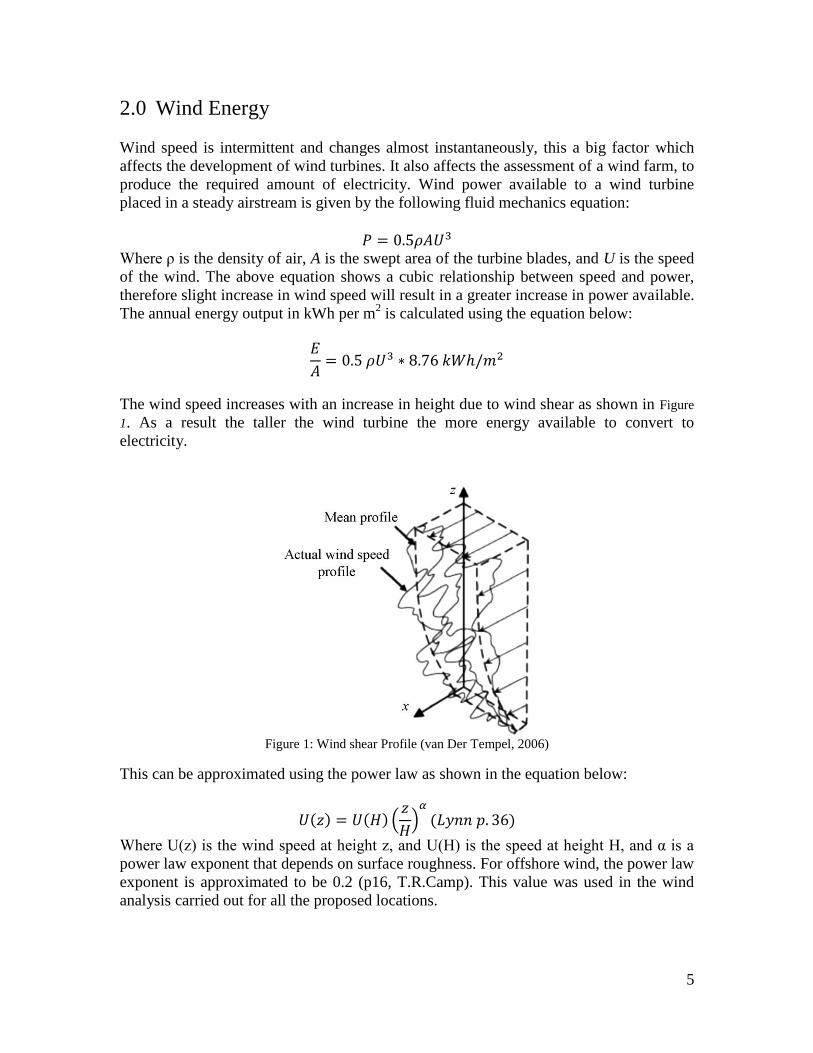
The wind speed increases with an increase in height due to wind shear as shown in Figure

1. As a result the taller the wind turbine the more energy available to convert to

electricity.

Figure 1: Wind shear Profile (van Der Tempel, 2006)

This can be approximated using the power law as shown in the equation below:

𝑈(𝑧) = 𝑈(𝐻) (𝑧

𝐻)

𝛼

(𝐿𝑦𝑛𝑛 𝑝. 36)

Where U(z) is the wind speed at height z, and U(H) is the speed at height H, and α is a

power law exponent that depends on surface roughness. For offshore wind, the power law

exponent is approximated to be 0.2 (p16, T.R.Camp). This value was used in the wind

analysis carried out for all the proposed locations.

6

The power available in the wind and wind shear profile change vary with locations.

Using wind data collected from a particular site, the above equations help analyze a site’s

viability for a productive wind farm. These are major factors used in site selection.

3.0 Site Selection Analysis

For an offshore wind turbine to capture as much wind power possible a suitable location

must be selected. The farm’s overall performance depends crucially on the conditions at

the particular site. Therefore the following features must be considered:

a. Proximity to the grid

b. Water Depth

c. Wind Energy Available (daily and seasonal)

These factors not only take into account the wind resource but also the projected

installation and maintenance costs of an offshore wind farm. Three sites, Sable Island,

Yarmouth and Shelburne were preliminarily chosen for analysis. This was based on the

availability of hourly wind data over the course of the year, proximity to the coast and

Nova Scotia wind atlas showing the average wind speeds.

Proximity to the Grid

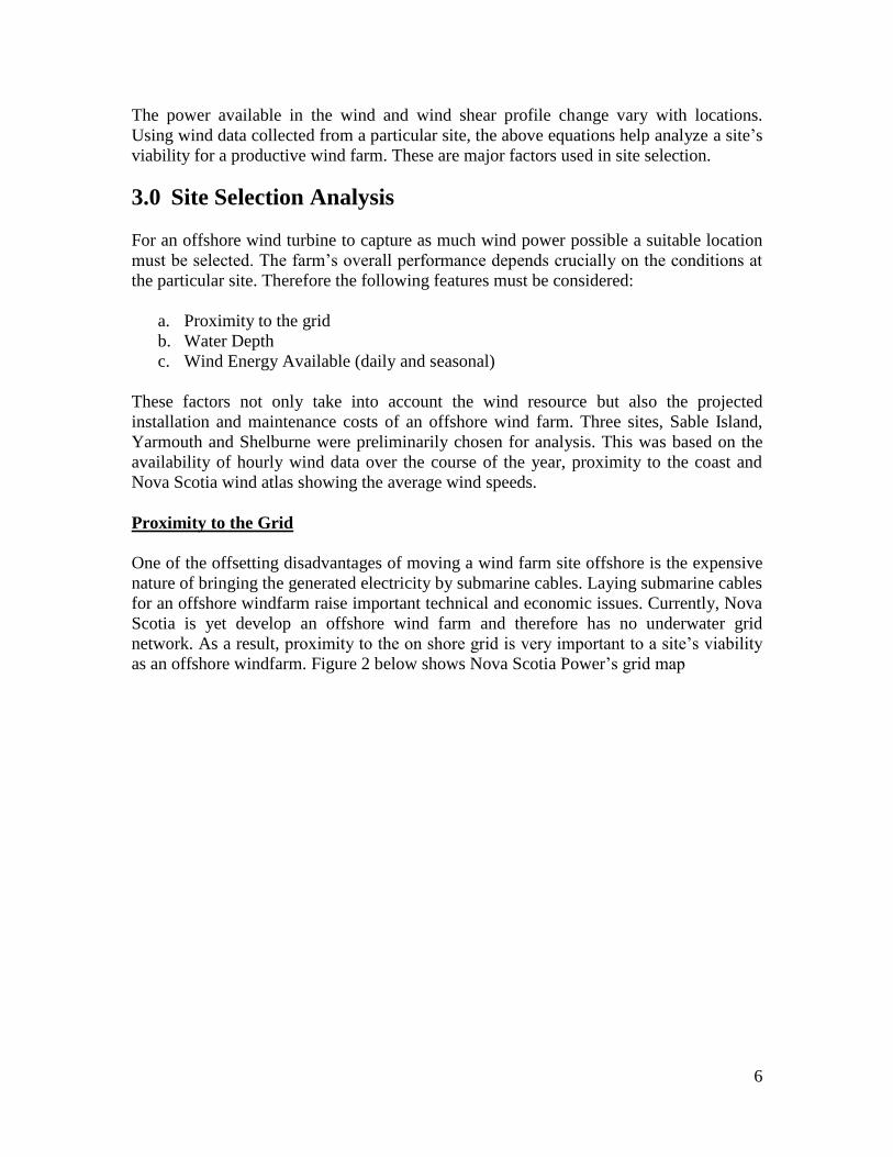
One of the offsetting disadvantages of moving a wind farm site offshore is the expensive

nature of bringing the generated electricity by submarine cables. Laying submarine cables

for an offshore windfarm raise important technical and economic issues. Currently, Nova

Scotia is yet develop an offshore wind farm and therefore has no underwater grid

network. As a result, proximity to the on shore grid is very important to a site’s viability

as an offshore windfarm. Figure 2 below shows Nova Scotia Power’s grid map

7

Figure 2: Nova Scotia transmission and distribution map

Figure 2 shows the close proximity of the proposed Yarmouth and Shelburne offshore

locations to Nova Scotia’s grid.

Sable Island is a small island situated about 300 km south east of Halifax. It is also a

protected National Park Reserve. An offshore wind farm in close proximity to Sable

Island will require installation of at least 300 km of subsea high-voltage direct current

cables thereby increasing the construction costs. Laying such cable cost ~ $1M/km. This

makes Sable Island a less than ideal location for an offshore wind farm based on its

projected construction costs. In addition, a proposed wind farm would have undergo a

vigorous Federal Environmental Assessment process as it is part of a key migratory

flyway, with numerous bird species with over 350 recorded, such as the Roseate Tern and

Ipswich Sparrow. An offshore wind farm in proximity to Sable Island could pose a threat

to the migratory birds.

In terms of projected construction costs, Yarmouth and Shelburne sites are more ideal

location for an offshore wind farm because of their close proximity to Nova Scotia’s

electricity grid.

Water Depth

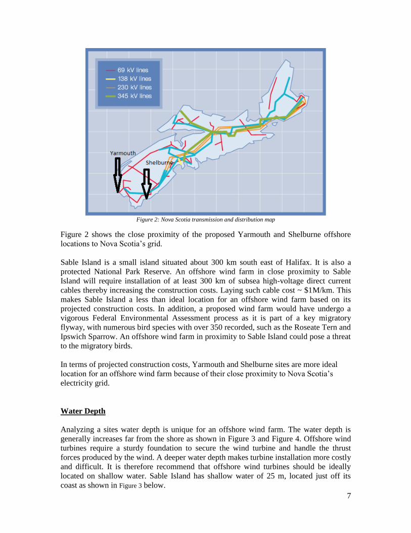
Analyzing a sites water depth is unique for an offshore wind farm. The water depth is

generally increases far from the shore as shown in Figure 3 and Figure 4. Offshore wind

turbines require a sturdy foundation to secure the wind turbine and handle the thrust

forces produced by the wind. A deeper water depth makes turbine installation more costly

and difficult. It is therefore recommend that offshore wind turbines should be ideally

located on shallow water. Sable Island has shallow water of 25 m, located just off its

coast as shown in Figure 3 below.

8

Figure 3: Sable Island bathymetric chart (National Oceanic and Atmospheric Administration)

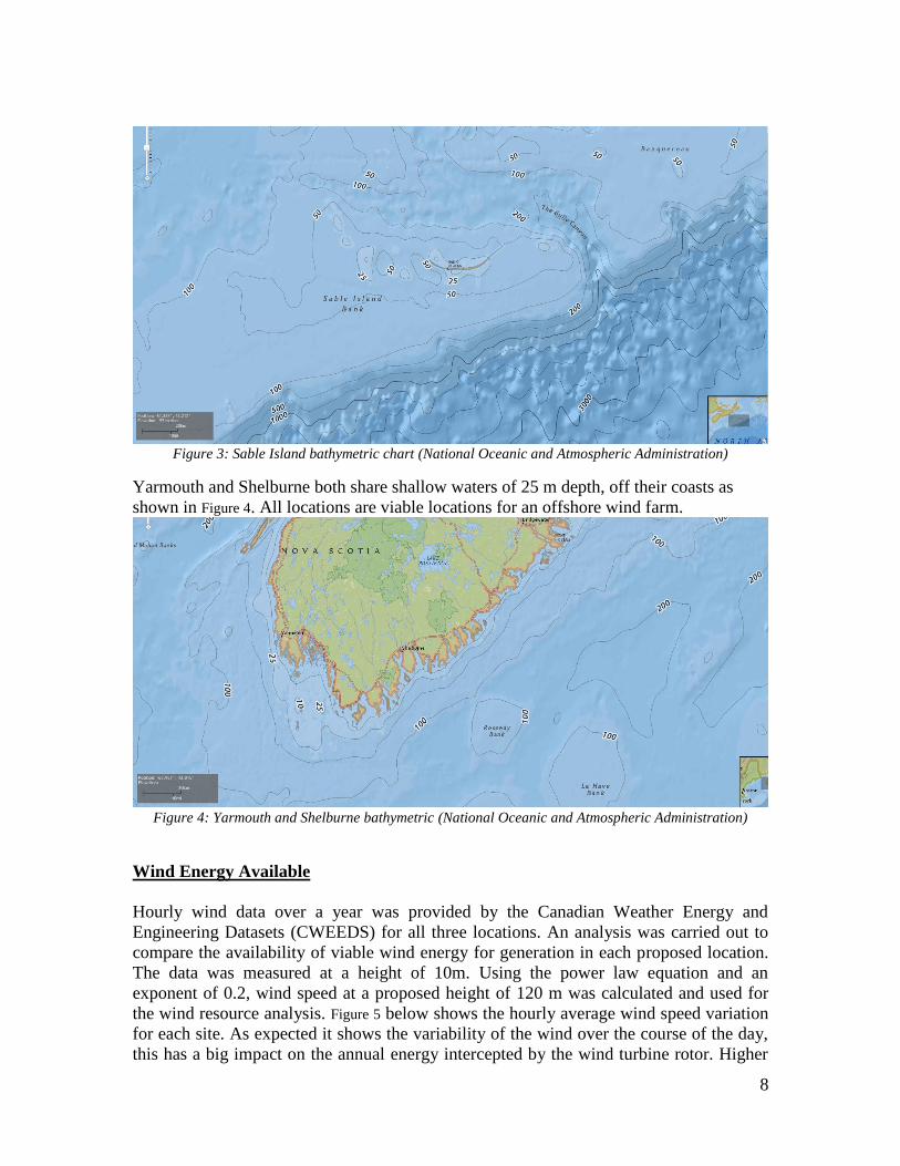
Yarmouth and Shelburne both share shallow waters of 25 m depth, off their coasts as

shown in Figure 4. All locations are viable locations for an offshore wind farm.

Figure 4: Yarmouth and Shelburne bathymetric (National Oceanic and Atmospheric Administration)

Wind Energy Available

Hourly wind data over a year was provided by the Canadian Weather Energy and

Engineering Datasets (CWEEDS) for all three locations. An analysis was carried out to

compare the availability of viable wind energy for generation in each proposed location.

The data was measured at a height of 10m. Using the power law equation and an

exponent of 0.2, wind speed at a proposed height of 120 m was calculated and used for

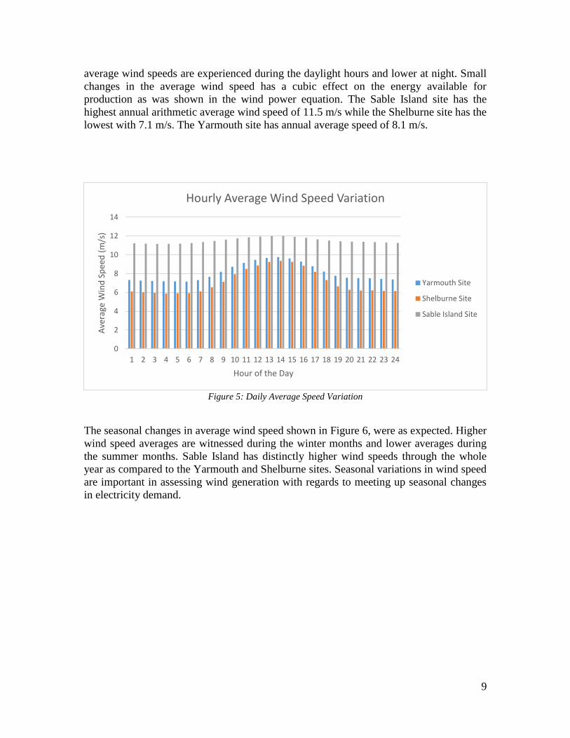
the wind resource analysis. Figure 5 below shows the hourly average wind speed variation

for each site. As expected it shows the variability of the wind over the course of the day,

this has a big impact on the annual energy intercepted by the wind turbine rotor. Higher

9

average wind speeds are experienced during the daylight hours and lower at night. Small

changes in the average wind speed has a cubic effect on the energy available for

production as was shown in the wind power equation. The Sable Island site has the

highest annual arithmetic average wind speed of 11.5 m/s while the Shelburne site has the

lowest with 7.1 m/s. The Yarmouth site has annual average speed of 8.1 m/s.

Figure 5: Daily Average Speed Variation

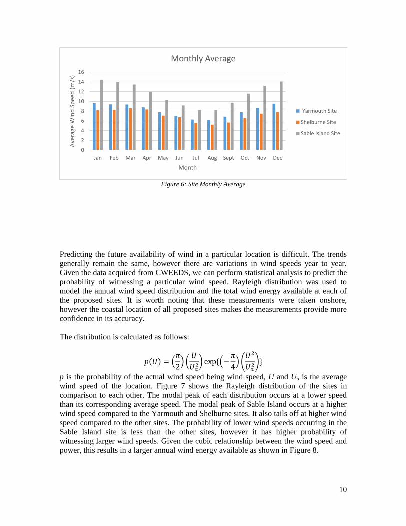
The seasonal changes in average wind speed shown in Figure 6, were as expected. Higher

wind speed averages are witnessed during the winter months and lower averages during

the summer months. Sable Island has distinctly higher wind speeds through the whole

year as compared to the Yarmouth and Shelburne sites. Seasonal variations in wind speed

are important in assessing wind generation with regards to meeting up seasonal changes

in electricity demand.

0

2

4

6

8

10

12

14

1 2 3 4 5 6 7 8 9 10 11 12 13 14 15 16 17 18 19 20 21 22 23 24

Ave

rage

Win

d S

pee

d (

m/s

)

Hour of the Day

Hourly Average Wind Speed Variation

Yarmouth Site

Shelburne Site

Sable Island Site

10

Figure 6: Site Monthly Average

Predicting the future availability of wind in a particular location is difficult. The trends

generally remain the same, however there are variations in wind speeds year to year.

Given the data acquired from CWEEDS, we can perform statistical analysis to predict the

probability of witnessing a particular wind speed. Rayleigh distribution was used to

model the annual wind speed distribution and the total wind energy available at each of

the proposed sites. It is worth noting that these measurements were taken onshore,

however the coastal location of all proposed sites makes the measurements provide more

confidence in its accuracy.

The distribution is calculated as follows:

𝑝(𝑈) = (𝜋

2) (

𝑈

𝑈𝑎2

) exp {(−𝜋

4) (

𝑈2

𝑈𝑎2

)}

p is the probability of the actual wind speed being wind speed, U and Ua is the average

wind speed of the location. Figure 7 shows the Rayleigh distribution of the sites in

comparison to each other. The modal peak of each distribution occurs at a lower speed

than its corresponding average speed. The modal peak of Sable Island occurs at a higher

wind speed compared to the Yarmouth and Shelburne sites. It also tails off at higher wind

speed compared to the other sites. The probability of lower wind speeds occurring in the

Sable Island site is less than the other sites, however it has higher probability of

witnessing larger wind speeds. Given the cubic relationship between the wind speed and

power, this results in a larger annual wind energy available as shown in Figure 8.

0

2

4

6

8

10

12

14

16

Jan Feb Mar Apr May Jun Jul Aug Sept Oct Nov Dec

Ave

rage

Win

d S

pee

d (

m/s

)

Month

Monthly Average

Yarmouth Site

Shelburne Site

Sable Island Site

11

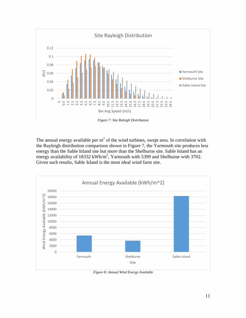
Figure 7: Site Raleigh Distribution

The annual energy available per m2 of the wind turbines, swept area. In correlation with

the Rayleigh distribution comparison shown in Figure 7, the Yarmouth site produces less

energy than the Sable Island site but more than the Shelburne site. Sable Island has an

energy availability of 18332 kWh/m2, Yarmouth with 5399 and Shelburne with 3702.

Given such results, Sable Island is the most ideal wind farm site.

Figure 8: Annual Wind Energy Available

0

0.02

0.04

0.06

0.08

0.1

0.12

00

.51

.52

.53

.54

.55

.56

.57

.58

.59

.51

0.5

11

.51

2.5

13

.51

4.5

15

.51

6.5

17

.51

8.5

19

.52

0.5

21

.52

2.5

23

.52

4.5

p(u

)

Bin Avg Speed (m/s)

Site Rayleigh Distribution

Yarmouth Site

Shelburne Site

Sable Island Site

0

2000

4000

6000

8000

10000

12000

14000

16000

18000

20000

Yarmouth Shelburne Sable Island

Win

d E

ner

gy A

vaila

ble

(kW

h/m

^2)

Site

Annual Energy Available (kWh/m^2)

12

The analysis of each site based on its proximity to the grid, water depth and availability

of wind energy has made Yarmouth an ideal location for a wind farm. All sites are ideal

based on water depth. Yarmouth is ideal primarily because it does not run into the

complexity of being a large distance away from the grid, thereby incurring large

construction and grid integration costs. This overrides Sable Island’s significantly larger

value of wind energy available. In addition, Yarmouth, has a higher amount of energy

available compared to the Shelburne site.

4.0 Turbine Selection

There are variety of wind turbine manufacturers in the world, choosing the appropriate

turbine is paramount to a wind farm’s ability to generate the required amount of

electricity, safely. A variety of parameters included in selecting the appropriate turbine,

however this is based mainly on the site conditions, and turbine performance. All this is

driven in large parts by the wind resource analysis performed in the previous section.

Selection based on Site Conditions

The turbine selected must be able to handle all the conditions of the Yarmouth site, whilst

generating a significant amount of electricity, based on the electricity demand. The

International Electromechanical Commission published an international standard, IEC

61400 regarding the engineering integrity of wind turbines based on site conditions. This

is to ensure that the wind turbine is protected from all hazards during its 25 year life cycle

(Wind Turbines). These site conditions include the maximum wind speed and turbulence

intensity. (Manuel et al, 41). The turbines are classified in 3 different categories for each

site condition as shown in Table 1.

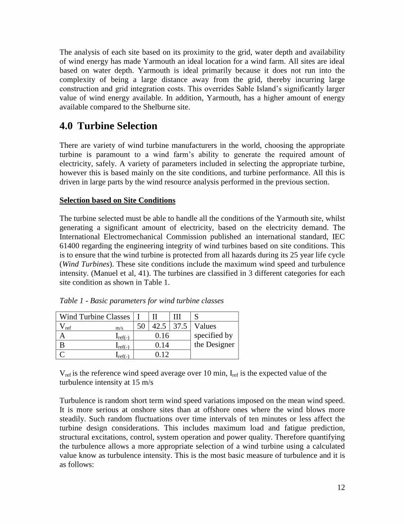
Table 1 - Basic parameters for wind turbine classes

Wind Turbine Classes I II III S

Vref m/s 50 42.5 37.5 Values

specified by

the Designer A Iref(-) 0.16

B Iref(-) 0.14

C Iref(-) 0.12

Vref is the reference wind speed average over 10 min, Iref is the expected value of the

turbulence intensity at 15 m/s

Turbulence is random short term wind speed variations imposed on the mean wind speed.

It is more serious at onshore sites than at offshore ones where the wind blows more

steadily. Such random fluctuations over time intervals of ten minutes or less affect the

turbine design considerations. This includes maximum load and fatigue prediction,

structural excitations, control, system operation and power quality. Therefore quantifying

the turbulence allows a more appropriate selection of a wind turbine using a calculated

value know as turbulence intensity. This is the most basic measure of turbulence and it is

as follows:

13

𝑇𝐼 =𝜎𝑢

𝑈

σu is the standard deviation. The turbulence intensity ranges from 0.1 to 0.4, with the

highest occurring at the lowest wind speeds (Manuel et al, 41) as shown in Figure 9. The

main consequence of increased turbulence is are increased thrust loads and fatigue on the

turbine blades.

Figure 9: Turbulence intensity for the normal turbulence model

The Yarmouth site conditions can be described based on the above parameters. The

maximum gust wind measured at the site was 49 m/s, therefore the wind turbine has to be

rated under Class I with a reference speed of 50 m/s. There is no data to accurately

quantify the turbulence intensity at this location. As a result a safe turbulence intensity of

0.16 is chosen, placing it under Class A. Given that the turbulence intensity is low on

offshore locations than onshore, a wind turbine rated for Class A is more than appropriate

for the site’s conditions. Therefore the wind turbine to be selected must have an IEC

Class of IA.

Turbine output

A turbine’s performance is usually characterized by its power coefficient, Cp:

𝐶𝑝 =𝑃

0.5𝜌𝑈3𝐴=

𝑃𝑜𝑤𝑒𝑟 𝑔𝑒𝑛𝑒𝑟𝑎𝑡𝑒𝑑

𝑃𝑜𝑤𝑒𝑟 𝑖𝑛 𝑡ℎ𝑒 𝑊𝑖𝑛𝑑

This non-dimensional value represents the fractional value of power in the wind that is

converted to electricity. It changes depending on the wind speed, U at the hub height. The

theoretical limit of rotor efficiency, named the Betz Limit was discovered to be 0.59. This

states that a rotor in a steady airstream cannot convert more than 59%, of the wind’s

14

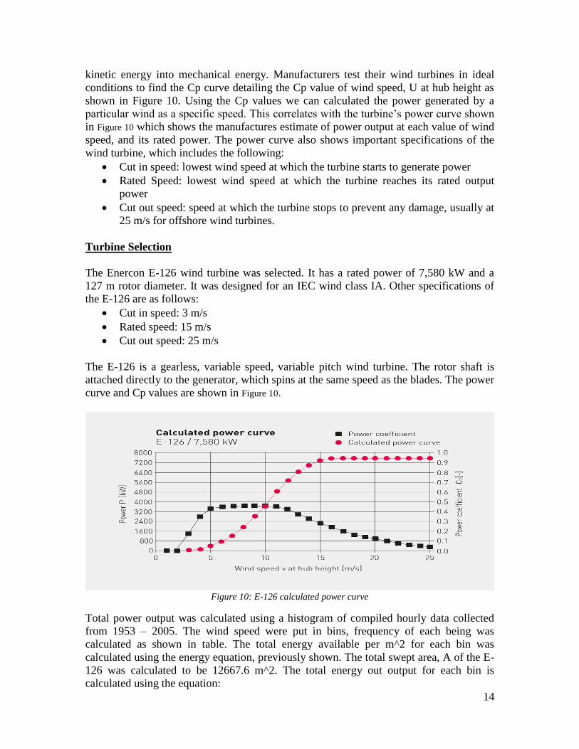
kinetic energy into mechanical energy. Manufacturers test their wind turbines in ideal

conditions to find the Cp curve detailing the Cp value of wind speed, U at hub height as

shown in Figure 10. Using the Cp values we can calculated the power generated by a

particular wind as a specific speed. This correlates with the turbine’s power curve shown

in Figure 10 which shows the manufactures estimate of power output at each value of wind

speed, and its rated power. The power curve also shows important specifications of the

wind turbine, which includes the following:

Cut in speed: lowest wind speed at which the turbine starts to generate power

Rated Speed: lowest wind speed at which the turbine reaches its rated output

power

Cut out speed: speed at which the turbine stops to prevent any damage, usually at

25 m/s for offshore wind turbines.

Turbine Selection

The Enercon E-126 wind turbine was selected. It has a rated power of 7,580 kW and a

127 m rotor diameter. It was designed for an IEC wind class IA. Other specifications of

the E-126 are as follows:

Cut in speed: 3 m/s

Rated speed: 15 m/s

Cut out speed: 25 m/s

The E-126 is a gearless, variable speed, variable pitch wind turbine. The rotor shaft is

attached directly to the generator, which spins at the same speed as the blades. The power

curve and Cp values are shown in Figure 10.

Figure 10: E-126 calculated power curve

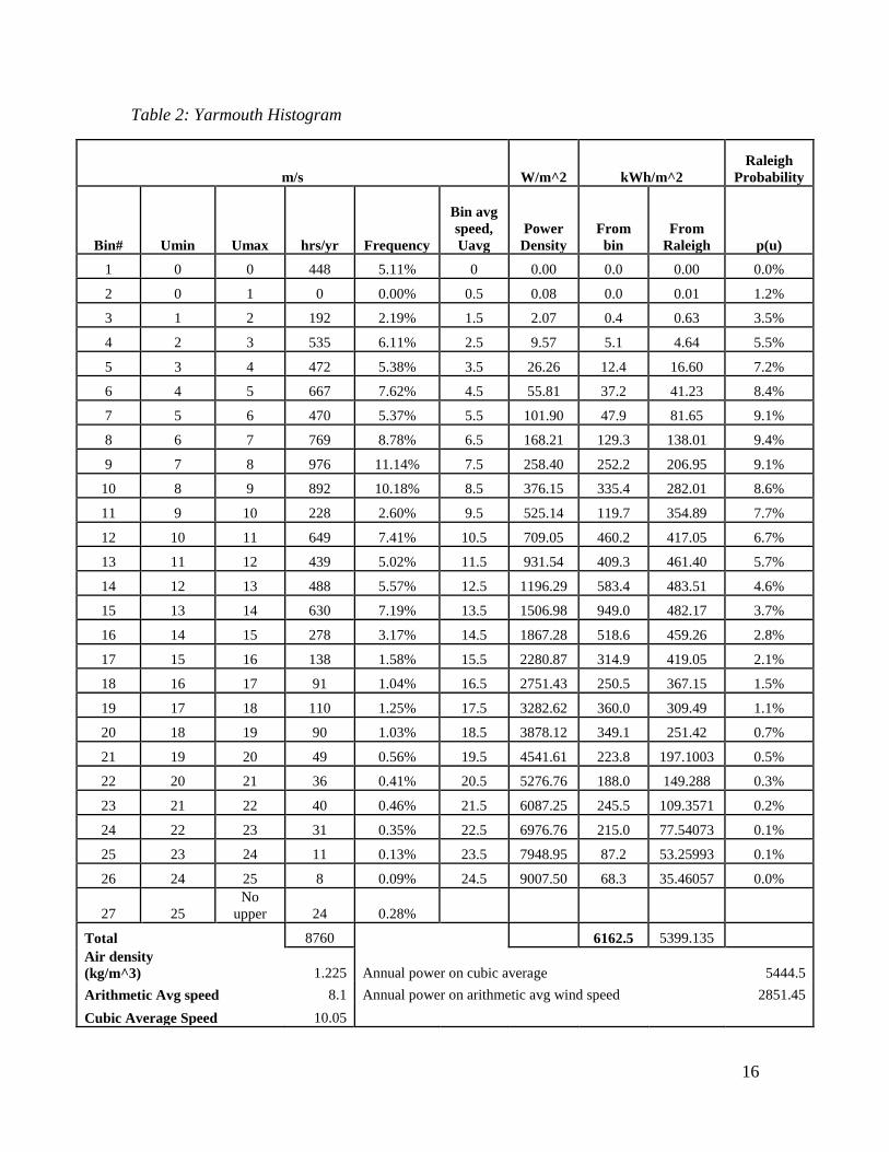
Total power output was calculated using a histogram of compiled hourly data collected

from 1953 – 2005. The wind speed were put in bins, frequency of each being was

calculated as shown in table. The total energy available per m^2 for each bin was

calculated using the energy equation, previously shown. The total swept area, A of the E-

126 was calculated to be 12667.6 m^2. The total energy out output for each bin is

calculated using the equation:

15

𝐸 = ∑ 𝐶𝑝 𝑏𝑖𝑛 ∗ (𝐸/𝐴)𝑏𝑖𝑛 ∗ 𝐴𝑡𝑢𝑟𝑏𝑖𝑛𝑒

The power coefficient of the bin, Cp bin corresponding to the bin average speed is shown

in Figure 10. The energy density for each bin, (E/A)bin is shown in Table 2.

16

Table 2: Yarmouth Histogram

m/s W/m^2 kWh/m^2

Raleigh

Probability

Bin# Umin Umax hrs/yr Frequency

Bin avg

speed,

Uavg

Power

Density

From

bin

From

Raleigh p(u)

1 0 0 448 5.11% 0 0.00 0.0 0.00 0.0%

2 0 1 0 0.00% 0.5 0.08 0.0 0.01 1.2%

3 1 2 192 2.19% 1.5 2.07 0.4 0.63 3.5%

4 2 3 535 6.11% 2.5 9.57 5.1 4.64 5.5%

5 3 4 472 5.38% 3.5 26.26 12.4 16.60 7.2%

6 4 5 667 7.62% 4.5 55.81 37.2 41.23 8.4%

7 5 6 470 5.37% 5.5 101.90 47.9 81.65 9.1%

8 6 7 769 8.78% 6.5 168.21 129.3 138.01 9.4%

9 7 8 976 11.14% 7.5 258.40 252.2 206.95 9.1%

10 8 9 892 10.18% 8.5 376.15 335.4 282.01 8.6%

11 9 10 228 2.60% 9.5 525.14 119.7 354.89 7.7%

12 10 11 649 7.41% 10.5 709.05 460.2 417.05 6.7%

13 11 12 439 5.02% 11.5 931.54 409.3 461.40 5.7%

14 12 13 488 5.57% 12.5 1196.29 583.4 483.51 4.6%

15 13 14 630 7.19% 13.5 1506.98 949.0 482.17 3.7%

16 14 15 278 3.17% 14.5 1867.28 518.6 459.26 2.8%

17 15 16 138 1.58% 15.5 2280.87 314.9 419.05 2.1%

18 16 17 91 1.04% 16.5 2751.43 250.5 367.15 1.5%

19 17 18 110 1.25% 17.5 3282.62 360.0 309.49 1.1%

20 18 19 90 1.03% 18.5 3878.12 349.1 251.42 0.7%

21 19 20 49 0.56% 19.5 4541.61 223.8 197.1003 0.5%

22 20 21 36 0.41% 20.5 5276.76 188.0 149.288 0.3%

23 21 22 40 0.46% 21.5 6087.25 245.5 109.3571 0.2%

24 22 23 31 0.35% 22.5 6976.76 215.0 77.54073 0.1%

25 23 24 11 0.13% 23.5 7948.95 87.2 53.25993 0.1%

26 24 25 8 0.09% 24.5 9007.50 68.3 35.46057 0.0%

27 25

No

upper 24 0.28%

Total 8760 6162.5 5399.135

Air density

(kg/m^3)

1.225 Annual power on cubic average 5444.5

Arithmetic Avg speed 8.1 Annual power on arithmetic avg wind speed 2851.45

Cubic Average Speed 10.05

17

The annual energy output for an E-126 turbine was calculated to be 23.6 GWh. The

average value of Cp is 0.30.

Site Specification

• Location: Yarmouth

• Distance off the coast: 20 km

• Average wind speed: 8.1 m/s

• Annual Energy Output per turbine = 23.6 GWh

• No of units: 14

• Nameplate capacity: 101.92 MW

• Total Energy Output: 330.4 GWh

• CO2 offset: 323931 g of CO2 (coal)

• Number of households: 32797

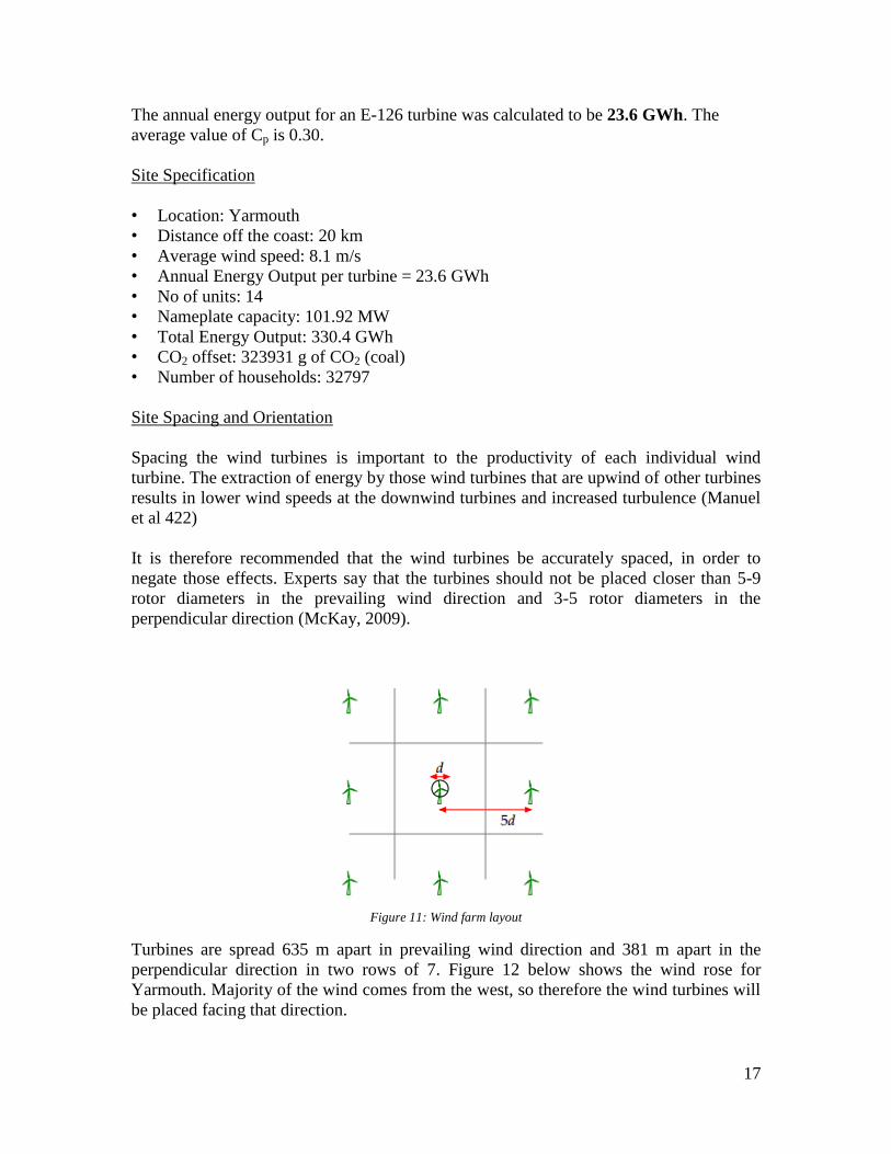
Site Spacing and Orientation

Spacing the wind turbines is important to the productivity of each individual wind

turbine. The extraction of energy by those wind turbines that are upwind of other turbines

results in lower wind speeds at the downwind turbines and increased turbulence (Manuel

et al 422)

It is therefore recommended that the wind turbines be accurately spaced, in order to

negate those effects. Experts say that the turbines should not be placed closer than 5-9

rotor diameters in the prevailing wind direction and 3-5 rotor diameters in the

perpendicular direction (McKay, 2009).

Figure 11: Wind farm layout

Turbines are spread 635 m apart in prevailing wind direction and 381 m apart in the

perpendicular direction in two rows of 7. Figure 12 below shows the wind rose for

Yarmouth. Majority of the wind comes from the west, so therefore the wind turbines will

be placed facing that direction.

18

Figure 12: Yarmouth Wind Rose

4.1. Offshore wind turbine support structure

The support structure of the offshore wind turbine is responsible for fixing the turbine in

place and keeping it upright. This type of structure is subjected to highly dynamic loads

due to the combined wind and hydrodynamic loading and the complex dynamic loading

from the wind turbine. When designing a support structure for an offshore wind turbine

it is crucial to accurately capture the effects of wind loads, wave loads, and dynamic

loading from the turbine. The reason for this is due to total loading likely being much

smaller than the sum of each consecutive load, since the loads are not coincident and

aerodynamic damping from the rotor greatly damps motion from wave loading. Several

types of support structures were looked into for designing the wind turbine in Yarmouth,

it was decided that a monopile design would be the best choice. The monopile foundation

was chosen due to its simplicity in design, ease of manufacture, and from it being the

cheapest foundation option.

The monopile foundation

The monopile foundation is the most common type of support structure installed with

offshore wind turbines, the European Offshore Statistics Association reported that 97%

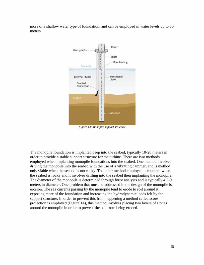
foundations installed in 2015 were monopiles. The design of the monopile foundation is

relatively simple; it is a cylindrical foundation pile with a transition piece that connects

the turbine tower and monopile (Figure 13). It is important to note that monopiles are

N

NE

E

SE

S

SW

W

NW

Yarmouth Wind Rose

19

more of a shallow water type of foundation, and can be employed in water levels up to 30

meters.

Figure 13: Monopile support structure

The monopile foundation is implanted deep into the seabed, typically 10-20 meters in

order to provide a stable support structure for the turbine. There are two methods

employed when implanting monopile foundations into the seabed. One method involves

driving the monopile into the seabed with the use of a vibrating hammer, and is method

only viable when the seabed is not rocky. The other method employed is required when

the seabed is rocky and it involves drilling into the seabed then implanting the monopile.

The diameter of the monopile is determined through force analysis and is typically 4.5-9

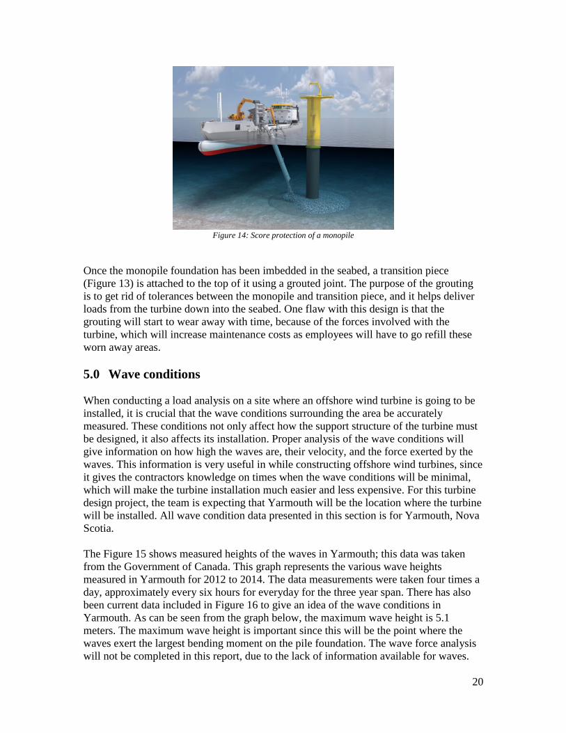
meters in diameter. One problem that must be addressed in the design of the monopile is

erosion. The sea currents passing by the monopile tend to erode to soil around it,

exposing more of the foundation and increasing the hydrodynamic loads felt by the

support structure. In order to prevent this from happening a method called score

protection is employed (Figure 14), this method involves placing two layers of stones

around the monopile in order to prevent the soil from being eroded.

20

Figure 14: Score protection of a monopile

Once the monopile foundation has been imbedded in the seabed, a transition piece

(Figure 13) is attached to the top of it using a grouted joint. The purpose of the grouting

is to get rid of tolerances between the monopile and transition piece, and it helps deliver

loads from the turbine down into the seabed. One flaw with this design is that the

grouting will start to wear away with time, because of the forces involved with the

turbine, which will increase maintenance costs as employees will have to go refill these

worn away areas.

5.0 Wave conditions

When conducting a load analysis on a site where an offshore wind turbine is going to be

installed, it is crucial that the wave conditions surrounding the area be accurately

measured. These conditions not only affect how the support structure of the turbine must

be designed, it also affects its installation. Proper analysis of the wave conditions will

give information on how high the waves are, their velocity, and the force exerted by the

waves. This information is very useful in while constructing offshore wind turbines, since

it gives the contractors knowledge on times when the wave conditions will be minimal,

which will make the turbine installation much easier and less expensive. For this turbine

design project, the team is expecting that Yarmouth will be the location where the turbine

will be installed. All wave condition data presented in this section is for Yarmouth, Nova

Scotia.

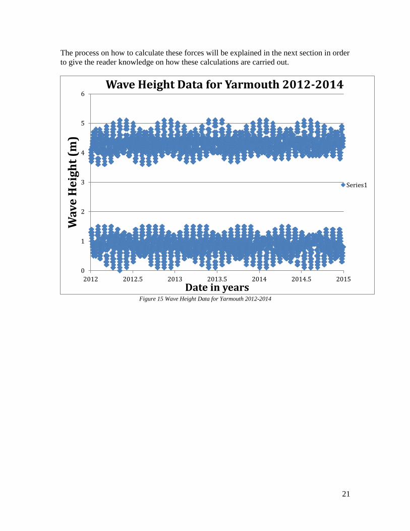
The Figure 15 shows measured heights of the waves in Yarmouth; this data was taken

from the Government of Canada. This graph represents the various wave heights

measured in Yarmouth for 2012 to 2014. The data measurements were taken four times a

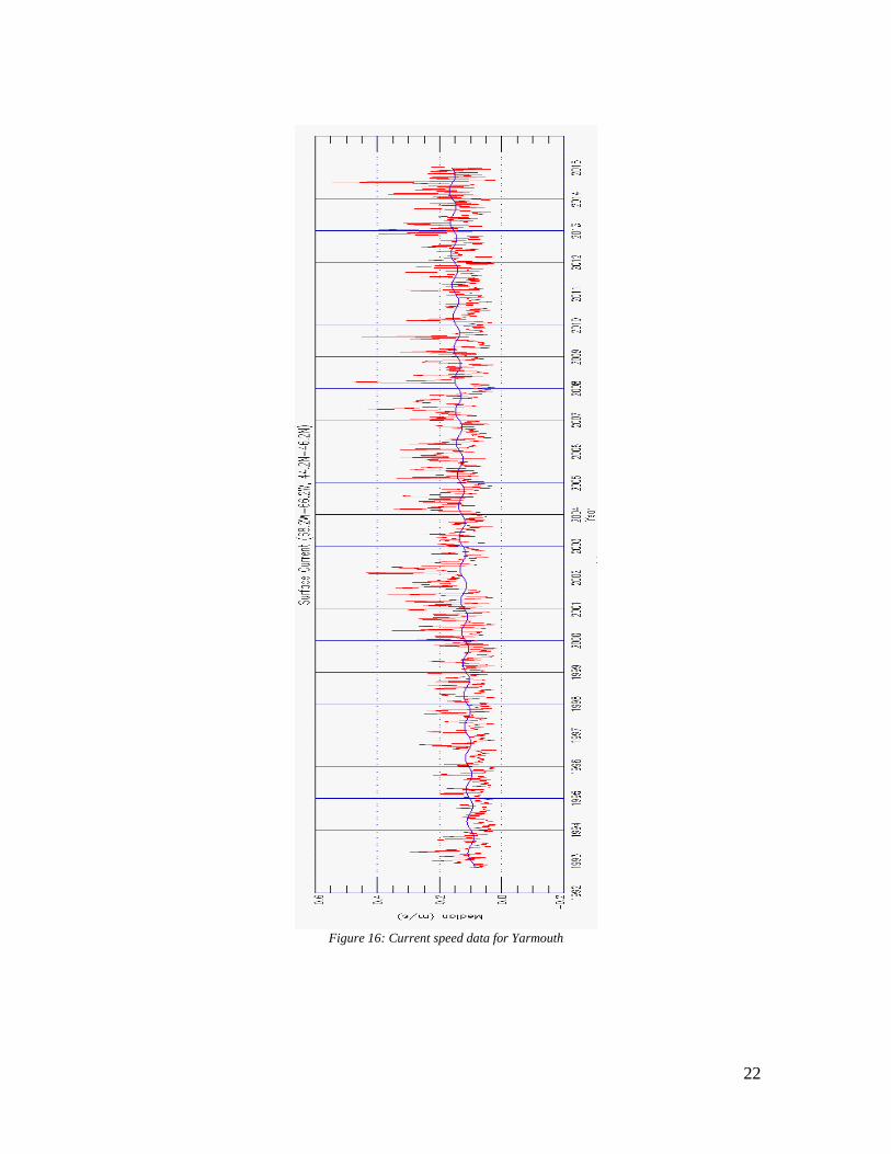
day, approximately every six hours for everyday for the three year span. There has also

been current data included in Figure 16 to give an idea of the wave conditions in

Yarmouth. As can be seen from the graph below, the maximum wave height is 5.1

meters. The maximum wave height is important since this will be the point where the

waves exert the largest bending moment on the pile foundation. The wave force analysis

will not be completed in this report, due to the lack of information available for waves.

21

The process on how to calculate these forces will be explained in the next section in order

to give the reader knowledge on how these calculations are carried out.

Figure 15 Wave Height Data for Yarmouth 2012-2014

0

1

2

3

4

5

6

2012 2012.5 2013 2013.5 2014 2014.5 2015

Wav

e H

eig

ht

(m)

Date in years

Wave Height Data for Yarmouth 2012-2014

Series1

22

Figure 16: Current speed data for Yarmouth

23

Wave Force Analysis

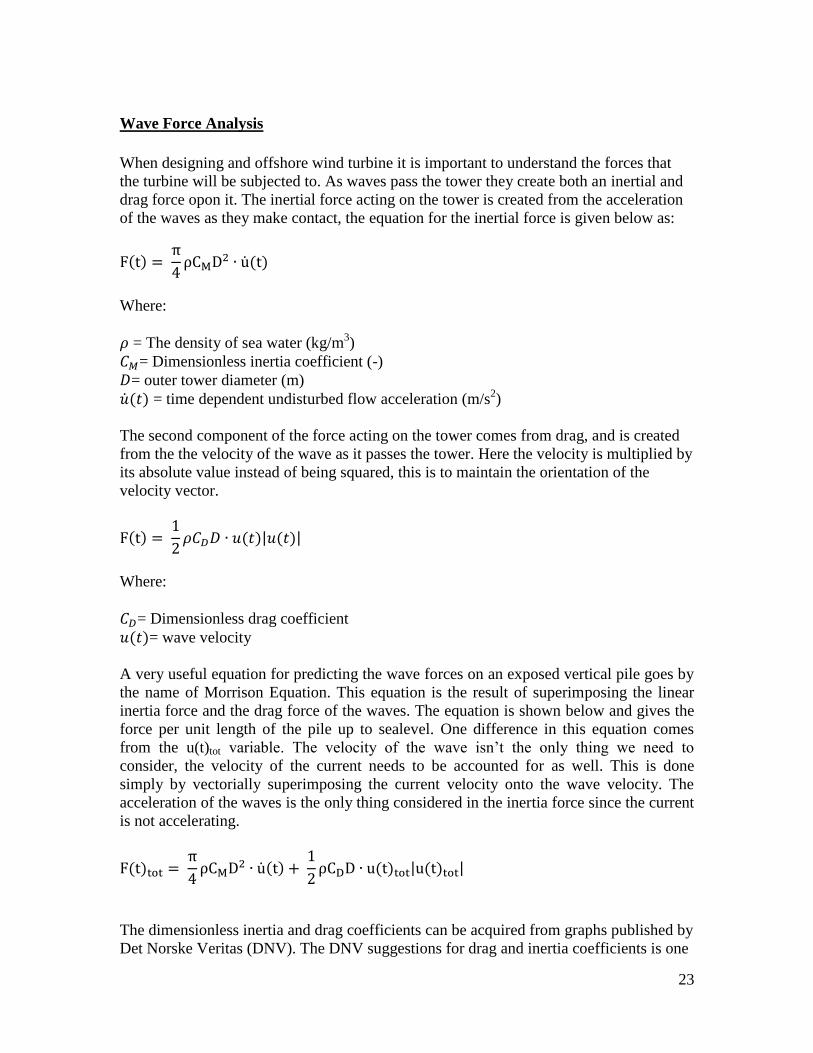
When designing and offshore wind turbine it is important to understand the forces that

the turbine will be subjected to. As waves pass the tower they create both an inertial and

drag force opon it. The inertial force acting on the tower is created from the acceleration

of the waves as they make contact, the equation for the inertial force is given below as:

F(t) = π

4ρCMD2 ∙ u̇(t)

Where:

𝜌 = The density of sea water (kg/m3)

𝐶𝑀= Dimensionless inertia coefficient (-)

𝐷= outer tower diameter (m)

�̇�(𝑡) = time dependent undisturbed flow acceleration (m/s2)

The second component of the force acting on the tower comes from drag, and is created

from the the velocity of the wave as it passes the tower. Here the velocity is multiplied by

its absolute value instead of being squared, this is to maintain the orientation of the

velocity vector.

F(t) = 1

2𝜌𝐶𝐷𝐷 ∙ 𝑢(𝑡)|𝑢(𝑡)|

Where:

𝐶𝐷= Dimensionless drag coefficient

𝑢(𝑡)= wave velocity

A very useful equation for predicting the wave forces on an exposed vertical pile goes by

the name of Morrison Equation. This equation is the result of superimposing the linear

inertia force and the drag force of the waves. The equation is shown below and gives the

force per unit length of the pile up to sealevel. One difference in this equation comes

from the u(t)tot variable. The velocity of the wave isn’t the only thing we need to

consider, the velocity of the current needs to be accounted for as well. This is done

simply by vectorially superimposing the current velocity onto the wave velocity. The

acceleration of the waves is the only thing considered in the inertia force since the current

is not accelerating.

F(t)tot = π

4ρCMD2 ∙ u̇(t) +

1

2ρCDD ∙ u(t)tot|u(t)tot|

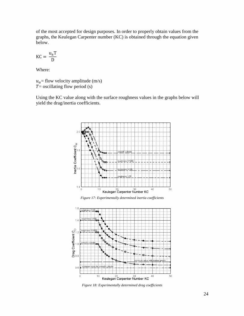
The dimensionless inertia and drag coefficients can be acquired from graphs published by

Det Norske Veritas (DNV). The DNV suggestions for drag and inertia coefficients is one

24

of the most accepted for design purposes. In order to properly obtain values from the

graphs, the Keulegan Carpenter number (KC) is obtained through the equation given

below.

KC = uaT

D

Where:

𝑢𝑎= flow velocity amplitude (m/s)

𝑇= oscillating flow period (s)

Using the KC value along with the surface roughness values in the graphs below will

yield the drag/inertia coefficients.

Figure 17: Experimentally determined inertia coefficients

Figure 18: Experimentally determined drag coefficients

25

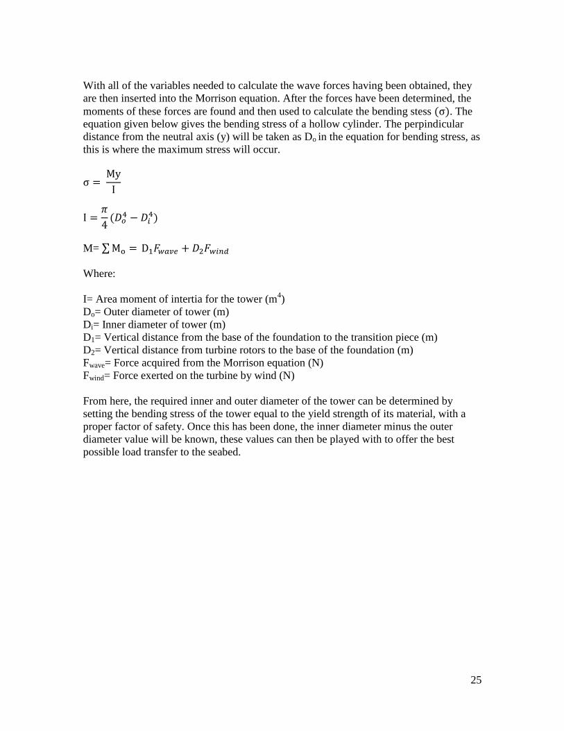
With all of the variables needed to calculate the wave forces having been obtained, they

are then inserted into the Morrison equation. After the forces have been determined, the

moments of these forces are found and then used to calculate the bending stess (σ). The

equation given below gives the bending stress of a hollow cylinder. The perpindicular

distance from the neutral axis (y) will be taken as Do in the equation for bending stress, as

this is where the maximum stress will occur.

σ = My

I

I =𝜋

4(𝐷𝑜

4 − 𝐷𝑖4)

M= ∑ Mo = D1𝐹𝑤𝑎𝑣𝑒 + 𝐷2𝐹𝑤𝑖𝑛𝑑

Where:

I= Area moment of intertia for the tower (m4)

Do= Outer diameter of tower (m)

Di= Inner diameter of tower (m)

D1= Vertical distance from the base of the foundation to the transition piece (m)

D2= Vertical distance from turbine rotors to the base of the foundation (m)

Fwave= Force acquired from the Morrison equation (N)

Fwind= Force exerted on the turbine by wind (N)

From here, the required inner and outer diameter of the tower can be determined by

setting the bending stress of the tower equal to the yield strength of its material, with a

proper factor of safety. Once this has been done, the inner diameter minus the outer

diameter value will be known, these values can then be played with to offer the best

possible load transfer to the seabed.

26

6.0 Finances

The mass of the wind turbine is just a small part of the cost of installing and maintaining

such a large piece of mechanical/electrical equipment. Shipping, machining,

transportation, all influence the total cost of each project. Furthermore, each project is

inherently different than other projects due to primarily, geographical location. Strictly

speaking, the geology of the ocean floor of the chosen location is not known. A steep,

rocky, location would make construction much more difficult than a flat bottom. The

geographical location, as well as the limited resources available on the Internet and the

limited number of offshore wind farms, an estimate of the cost can only be made.

The average cost of a wind turbine is approximately $1.3 to 2.2 million per MW (How

Much Do Wind Turbines Cost, 2016). The cost of preventative maintenance and

corrective maintenance can be as high as $10.00/MWh (Engels et al, 2009). In the same

report, listed is the maintenance cost for the Barrow offshore windfarm as $20.00/MWh.

The location of the Barrow wind farm relative to shore is similar to the chosen Yarmouth

location. At a depth of 18-22 m and a total energy output of 330 GWh it provides a good

measure of the maintenance costs for the proposed wind farm. According to another

report, construction costs can reach $4500 US/kW (RENEWABLE ENERGY

TECHNOLOGIES: COST ANALYSIS SERIES, 1992). Without going into too much

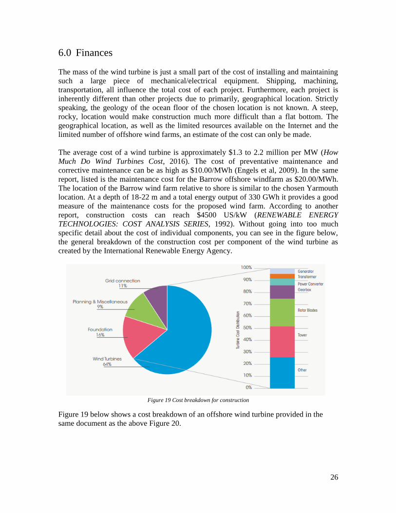
specific detail about the cost of individual components, you can see in the figure below,

the general breakdown of the construction cost per component of the wind turbine as

created by the International Renewable Energy Agency.

Figure 19 Cost breakdown for construction

Figure 19 below shows a cost breakdown of an offshore wind turbine provided in the

same document as the above Figure 20.

27

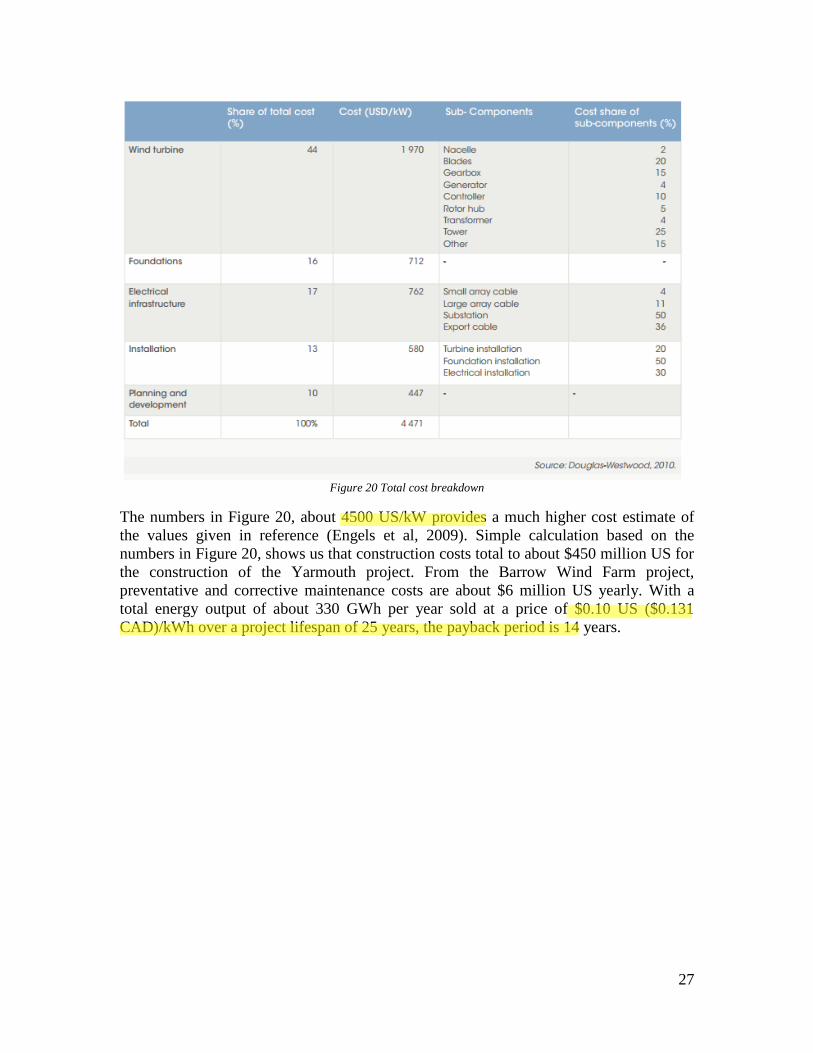
Figure 20 Total cost breakdown

The numbers in Figure 20, about 4500 US/kW provides a much higher cost estimate of

the values given in reference (Engels et al, 2009). Simple calculation based on the

numbers in Figure 20, shows us that construction costs total to about $450 million US for

the construction of the Yarmouth project. From the Barrow Wind Farm project,

preventative and corrective maintenance costs are about $6 million US yearly. With a

total energy output of about 330 GWh per year sold at a price of $0.10 US ($0.131

CAD)/kWh over a project lifespan of 25 years, the payback period is 14 years.

28

7.0 References

20% Wind Energy by 2030. US Department of Energy, July 2008. Web. 7 Mar. 2016.

Agarwal, Puneet, and Lance Manuel. "Wave Models for Offshore Wind Turbines."

American Institute of Aeronautics and Astronautics 1336 (2008): n. pag. Web.

"Current Funding Programs." Natural Resources Canada. Natural Resources Canada, 25

Feb. 2016. Web. 07 Mar. 2016.

Engels, Wouter, Tom Obdam, and Feike Savenije. Current Developments in Wind - 2009.

Tech. Energy Research Center in Netherlands, n.d. Web. 7 Mar. 2016.

"How Much Do Wind Turbines Cost?" Http://www.windustry.org/. N.p., n.d. Web. 7

Mar. 2016.

Lynn, Paul A. Onshore and Offshore Wind Energy: An Introduction. Chichester, West

Sussex: Wiley, 2012. Print.

Manuel, J. F., J. G. McGowan, and A. L. Rogers. Wind Energy Explained. 2nd ed. N.p.:

John Wiley & Sons, 2009. Print.

McKay, David. "Wind II." (n.d.): n. pag. Www.withouthotair.com. 2009. Web. 8 Mar.

2016.

"Renewable Energy Outlook." World Energy Outlook 2013 World Energy Outlook

(2013): 197-229. International Energy Agency, 2013. Web. 7 Mar. 2016.

"RENEWABLE ENERGY TECHNOLOGIES: COST ANALYSIS SERIES." Science

Scope 16.3 (1992): 32-34. International Renewable Energy Agency. Web. 8 Mar.

2016.

Report on the Review of the Community Feed-in Tariff Program. Halifax, N.S.: Dept. of

Energy, 2014. Mar. 2014. Web. 7 Mar. 2016.

29

"Sable Island National Park Reserve." Parks Canada. Parks Canada, Mar. 2012. Web. 8

Mar. 2016.

Wind Turbines – Part 1: Design Requirements. Tech. no. 61400-1. N.p.: International

Electrotechnical Commission, n.d. Print.

Miñambres, Oscar Yanguas. "Assessment of Current Offshore Wind Support Structures Concepts

– Challenges and Technological Requirements by 2020." Http://e-archivo.uc3m.es.

Karlshochschule International University. Web.

Espinosa, Julio García. "Design and Calculus of the Foundation Structure of an Offshore

Monopile Wind Turbine." Https://upcommons.upc.edu. Facultat De Nautica De

Barcelona, 1012. Web.

Marino, Enzo. "An Integrated Nonlinear Wind-Waves Model for Offshore Wind

Turbines." Google Books. Web. 08 Mar. 2016.

"Foundation Design Loa." Http://www.fema.gov. Web.

Techet, A. H. "Morrison's Equation." Http://web.mit.edu. MIT, 2004. Web.

"2015 Tide Tables." Government of Canada, Fisheries and Oceans Canada, Science.

Web. 08 Mar. 2016.

"Ocean Surface Currents (OSCAR)." Ocean Motion : Data Resources : Ocean Surface

Current Visualizer. Web. 08 Mar. 2016.

"The European Offshore Wind Industry - Key Trends and Statistics 2015."

Http://www.ewea.org. The European Wind Energy Association, Feb. 2016. Web.